Transition from inspiral to plunge for eccentric equatorial Kerr orbits

Abstract

Ori and Thorne have discussed the duration and observability (with LISA) of the transition from circular, equatorial inspiral to plunge for stellar-mass objects into supermassive ($10^{5}-10^{8}M_{\odot}$) Kerr black holes. We extend their computation to eccentric Kerr equatorial orbits. Even with orbital parameters near-exactly determined, we find that there is no universal length for the transition; rather, the length of the transition depends sensitively — essentially randomly — on initial conditions. Still, Ori and Thorne’s zero-eccentricity results are essentially an upper bound on the length of eccentric transitions involving similar bodies (e.g., $a$ fixed). Hence the implications for observations are no better: if the massive body is $M=10^{6}M_{\odot}$, the captured body has mass $m$, and the process occurs at distance $d$ from LISA, then $S/N\lesssim(m/10M_{\odot})(1\text{Gpc}/d)\times O(1)$, with the precise constant depending on the black hole spin. For low-mass bodies ($m\lesssim 7M_{\odot}$) for which the event rate is at least vaguely understood, we expect little chance (probably [much] less than $10\%$, depending strongly on the astrophysical assumptions) of LISA detecting a transition event with $S/N>5$ during its run; however, even a small infusion of higher-mass bodies or a slight improvement in LISA’s noise curve could potentially produce $S/N>5$ transition events during LISA’s lifetime.

I Introduction

The gravitational waves emitted during inspiral and infall of a body (mass $m$) into a black hole (mass $M$) should reveal detailed information about the orbital geometry and the hole’s spacetime geometry, thereby providing high-precision tests of general relativity Fintan . While the scattering of waves off background curvature implies that waves emitted at any time during the inspiral provide some small measure of even the smallest scale variations in the background spacetime geometry, the waves emitted as a particle passes through a region provide the most sensitive tests of that region: they reveal what path the particle has followed, and therefore constrain the spacetime to permit such a path. Therefore, to provide a sensitive probe of the innermost regions of black-hole spacetimes, we want to study orbits that pass as near as possible to the hole itself. Unfortunately, this means that the signals that are potentially the most informative about the hole’s innermost structure are typically the briefest: they arise from the end of the bound portion of the orbit and from the transition from inspiral to plunge. Since the relevant fraction of the orbit persists for only a small fraction of the overall detectable inspiral, we have significantly less probability to resolve waves during this interval than to resolve earlier, longer portions of the inspiral. One therefore wants to roughly characterize the waves emitted during these intervals (in the case of LISA sources, the goal of this paper). If this characterization suggests that planned observatories such as LIGO or LISA could detect them, one should then carry out much more detailed studies of these last few orbits and the waves they emit.

For inspirals appropriate to the LIGO band ($\sim 10$-$10^{3}$ Hz) and which LIGO can plausibly detect ($\eta=m/M$ $\sim 0.01$ to 1), order-of-magnitude computations (say, by post-Newtonian methods) suggest the last few waves are detectable ParametricFit . But because in this regime simple approximation techniques (such as post-Newtonian ParametricFit ; Alessandra ; KWW or test-particle approximations) break down, and because numerical relativity num1 codes remain incapable of evolving orbits accurately enough to find the waves, the community does not yet possess a waveform trusted for any purpose beyond detection.

LISA’s band ($\sim 10^{-3}$-$10^{-1}$Hz) will prove more sensitive to extreme mass-ratio infalls — that is, to stellar-mass black holes, white dwarfs, and neutron stars falling into supermassive [$M=O(10^{5}-10^{8})$, so $\eta\sim 10^{-4}$ to $10^{-8}$] black holes LISA . With such extreme mass ratios, the computation of detailed waveforms for purposes beyond mere detection should prove much simpler: to understand evolution, we need do nothing more than solve the classical radiation-reaction problem, albeit on a curved spacetime and with a gravitational, rather than electromagnetic, field reaction . While this problem hasn’t been solved to the accuracy required to construct long-integration-time coherent detection templates, one can employ adiabatic approximations to address most preliminary investigations. For example, as Ori and Thorne OriThorne have discussed in the context of circular inspiral, to understand the $\eta\ll 1$ transition’s duration — measured in experimentally observable gravitational wave cycles — we do not need a precise knowledge of the reaction force. An averaged reaction force —- one we can easily deduce from the radiation of conserved constants —- suffices for the short interval we will coherently employ it. Applying this reaction force, we can follow the particle through transition and thereby predict roughly how long this transition will last.

The goal of this paper is to extend the Ori-Thorne analysis to eccentric Kerr orbits, in an effort to estimate the prospects of LISA detecting a transition from inspiral to plunge.

This analysis relies on using the radiation of two conserved constants $E,L$ to compute the effect of radiation on the orbit. But for Kerr inclined orbits there is an additional constant — the Carter constant — whose evolution has not yet been related to fluxes at infinity. Since we lack the necessary tools, we leave the Kerr inclined case to a future paper.

I.1 Outline of this paper and summary of conclusions

In Sec. II, we will outline the basic physical framework behind our approach. In particular, we will introduce an explicit procedure to estimate the time duration of a transition. This procedure takes as input the net (time-averaged) fluxes of energy and angular momentum from the particle’s instantaneously geodesic orbits, input one obtains from a solution of the Teukolsky equation given a geodesic orbit as source. This procedure also takes as input some observationally-defined interpretation of what “the transition region” is. As the latter is ambiguous, and depends on exactly what sorts of templates one uses to find it, the exact length of the transition will depend on the convention one uses.

Ideally, one should define some unambiguous set of templates and match those against the simulated emitted waves to both define the transition duration and deduce the resulting signal-to-noise ratio for a given source. But for brevity and simplicity, as discussed in Sec. III, we will use a much cruder scheme — based on a purely sinusoidal, quadrupolar model for the waves — to characterize the expected LISA signal-to-noise ratio from a specific transition crossing. Given $S/N$ for an event and loosely-understood rates for transition events, we then develop, in Sec. III, a scheme for estimating the probability that LISA will see an event with $S/N$ greater than some detection threshold.

With this complete scheme for estimating the signal-to-noise of a characteristic source and determining the probability that LISA, in its currently-planned configuration, will see something, in Sec. IV and Sec. V we will apply it to inspirals into Schwarzchild and Kerr holes, respectively. We find in Sec. V.4 that Ori and Thorne’s zero-eccentricity results are essentially an upper bound on the length of eccentric transitions involving similar bodies (e.g., $a$ fixed). It follows, in Sec. V.5, that if we accept current (rough) astrophysical estimates of the masses and numbers of inspiralling stellar-mass black holes and if we employ only the current LISA design, we expect LISA will not see any transitions from inspiral to plunge during its lifetime, though it may come close.

Slight changes in LISA could make some transitions detectable. Dramatic improvements would be required to render LISA sensitive to prograde inspirals of stellar-mass black holes into rapidly-spinning ($a>0.9$) supermassive holes. But assuming such inspirals are a small proportion of all inspirals, if the LISA noise curve is lowered by a factor 3 (as is under currently discussion for other reasons), or if nature provides black holes more massive than $10M_{\odot}$ (say $30M_{\odot}$) in numbers approaching current estimates for $10M_{\odot}$, LISA would have a good chance of seeing one or two transitions sometime during its lifetime.

II Physical framework underlying the transition length estimate

In the (formal) absence of radiation reaction, a particle in equatorial orbit about a Kerr hole moves along a geodesic. Its radial motion can be determined from a first integral of the geodesic equation (equivalent to conservation of rest mass; see comments in Appendix A) MTW :

$$\left(\frac{dr}{d\tau}\right)^{2}+V\left[r\left(\tau\right),E,L\right]=0,$$ (1)

$$V\equiv-\left(E^{2}-1\right)-\frac{2}{r}+\frac{\left(L^{2}-a^{2}\left(E^{2}-1\right)\right)}{r^{2}}-\frac{2\left(L-aE\right)^{2}}{r^{3}}.$$ (2)

Here and throughout this paper all all quantities are, for simplicity, made dimensionless using the particle’s mass $m$ and the hole’s mass $M$: $E=$(orbital energy)/$m$, $L=$(orbital angular momentum)/$mM$, $r=$(orbital boyer-lindquist radius)/$M$, $\tau=$ (particle’s proper time)/$M$, and $a=$ (hole spin angular momentum)/$M^{2}$. Physical solutions may be specified by ($E$,$L$) or by any other pair of equivalent orbital parameters. It is conventional in the inspiral literature to employ as alternatives the parameters $p$ (a relativistic generalization of semi-latus rectum) and $e$ (a relativistic generalization of orbital eccentricity) CKP ; Dan ; these parameters are discussed in more detail in Appendix B.

We concern ourselves with a region of parameter space for which the maximum $V_{\text{max}}$ of the potential is nearly 0 (Fig. 1) and which therefore nearly admits a circular orbit at the radius $r_{\text{max}}$ of the maximum. The geodesic equation Eq. (1) implies that particles can spend an extremely (logarithmically) long time near the maximum; i.e. the particle can “whirl” several times about the hole in angle without moving significantly in $r$. It is conventional to call this portion of the orbit the “whirl.”

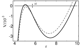
Figure 1: The effective potential $V(r,E,L)$ for radial geodesic motion gradually evolves during inspiral. If the initial eccentricity is nonzero, the maximum of the potential will gradually decrease until it passes below zero, thus permitting the particle to fall into the hole. By way of illustration, we plot $V(r,E,L)$ for $a=0$ and (solid) ($E$,$L$)=(0.948157, 3.53038) and (dashed) ($E$,$L$) =(0.947454, 3.52092). Under the action of radiation reaction, if $\eta=2\times 10^{-3}$ (an exaggerated mass ratio) the first system will evolve into the second after one radial period (of the first potential).

In the presence of radiation reaction (henceforth assumed weak), we must add to the geodesic equation (gauge-dependent) time-varying terms which reflect the (gauge-dependent) influence of gravitational radiation on the test particle’s path. These gauge-dependent terms oscillate on the same characteristic timescale as the radiation field. Since the radiation field is predominantly produced during the whirl part of the orbit, the radiation field predominantly oscillates at harmonics of the angular frequency $\Omega$ of circular orbits at the maximum. By averaging these reaction forces over a few cycles (e.g., over times $\approx 2\pi/\Omega$) to obtain their secular effect, we in principle find expressions for $E(\tau)$ and $L(\tau)$. Since the averaging time can still (particularly when the particle whirls several times about the hole) be shorter than the time the particle spends whirling around the central hole, we can to a good approximation employ Eq. (1) with time-varying $E(\tau)$, $L(\tau)$ to follow the orbit when the particle is near the maximum of the potential – and in particular the interval in which the particle goes from nearly-geodesic bound orbit into rapid plunge into the hole.

In this paper, we do not compute $E(\tau)$ and $L(\tau)$ in the thorough, general manner described here. See Sec. II.4 for a discussion of what information about $E(t)$ and $L(t)$ is required for our estimate and how that information is obtained.

II.1 Why we may still approximate the potential as static when computing the radial orbit

According to Eq. (1), a test particle on an approach to a black hole will fall into the hole if the local maximum of $V$,

$$I\equiv-V(r_{\max})=-V_{\text{max}}\;,$$ (3)

is negative. Radiation reaction reduces the local maximum faster than this potential $V$ flattens out. As the maximum decreases, the particle spends ever-more of its radial cycle near the local maximum. Eventually, we reach configurations such as those shown in Fig. 1, where the particle can slip over the maximum and fall into the black hole.

While configurations with $I\approx 0$ appear delicately balanced and therefore highly sensitive to small changes in $(E,L$), in fact under weak conditions (conditions made more explicit in Sec. II.3) one may ignore radiation reaction when computing a radial orbit and treat the potential $V$ as static.

Suppose a particle starts its whirl with some values for $(E,L)$ (and therefore $I$). During the whirl, even though $(E,L)$ change, the peak of the potential ($I$) will not change significantly (see Appendix A). Moreover, the location of the peak usually moves slowly relative to the particle. A condition for when the latter holds is presented in Sec. II.3. Therefore, during the whirl one can ignore radiation reaction.

After the particle finishes whirling about the hole, it moves outward to its outer radial turning point and back. During this period, the maximum does change, from $I$ to $I^{\prime}=I+\Delta I$. Unless the potential is nearly flat, however, the potential away from the neighborhood of the hole will not change much as $(E,L)$ change. Again, a condition for when the latter holds is presented in Sec. II.3. Therefore, in this interval one can again ignore radiation reaction.

When we attempt to evolve the particle through the next “whirl”, we need the correct value of the height of the maximum (now $I^{\prime}=I+\Delta I$) to determine how long the particle whirls around the hole. Therefore, when we start the cycle anew, we must use a potential with parameters $(E+\Delta E,L+\Delta L)$, with $\Delta E$ and $\Delta L$ the change in these constants over the preceeding full radial period. If $I^{\prime}<0$, the particle will “bounce” off the maximum and we repeat the cycle above once more. But eventually we will have $I^{\prime}>0$, at which point the particle will move across the maximum during its whirl and will subsequently “plunge” into the hole.

To summarize: so long as the potential is approximately static (cf. Sec. II.3), we expect we can understand transitions from inspiral to plunge by way of examining the geodesic equation [Eq. (1)] in the neighborhood of the local maximum, using $I\in[0,\Delta I]$.

II.2 Adiabatic approach to estimating the duration of the transition from inspiral to plunge

So long as we can treat the potential as static, we can approximate Eq. (1) in the neighborhood of the potential’s maximum at $r=r_{\text{max}}$ by the form

$$\gamma^{2}\left(\frac{d\delta r}{dt}\right)^{2}+\frac{\delta r^{2}}{\tau_{o}^{2}}=I.$$ (4)

Here $\delta r\equiv r-r_{\max}$; $r_{\max}$ is the instantaneously static location of the local maximum of $V$, and also the point about which we have expanded the potential;

$$\tau_{0}\equiv(V^{\prime\prime}/2)^{-1/2}$$ (5)

is a constant related to the curvature of the potential at the transition location; $t$ is the (dimensionless) time at infinity; and $\gamma$ is the redshift factor relating proper time $\tau$ to Boyer-lindquist coordinate time at $r=r_{\max}$:

$$\gamma=dt/d\tau{}_{r=r_{\text{max}}}\;.$$ (6)

Estimating the duration of a given transition: Solutions to Eq. (4 give hyperbolic motion; for example, the solution appropriate to $I>0$ is

$$r(t)-r_{\max}\approx\sqrt{I}\tau_{0}\sinh t/(\tau_{0}\gamma)\;.$$ (7)

Using this solution, we conclude that the transition time going from $r-r_{\max}=-\delta r_{\text{ref}}$ to $r-r_{\max}=\delta r_{\text{ref}}$ is

$$T_{c}(\delta r_{\text{ref}},I) \approx 2\gamma\tau_{o}\sinh^{-1}\left[\delta r_{\text{ref}}/(\tau_{o}\sqrt{I})\right]$$

$$\approx 2\gamma\tau_{o}\ln\left[2\delta r_{\text{ref}}/(\tau_{o}\sqrt{I})\right]$$

Hence given $\delta r_{\text{ref}}$, a quantity which defines what we mean by “the transition extent”, we can estimate the length of any transition (characterized by $I$) at any transition location (characterized by the explicit values that go into $\gamma$, $\tau_{o}$).

Estimating the distribution of transition durations: There is no unique transition duration. Rather, we have a distribution of durations, depending on the distribution of $I$ at the start of the particle’s final whirl. But that distribution is simple: since an initial configuration of particles will have some distribution of $I$, since this distribution evolves smoothly with no “knowledge” of the preferred scale $\Delta I$, and since $\Delta I$ will be smaller than any scale in the distribution function, a test particle on its final, plunge-triggering whirl has an approximately equal probability to have any $I\in[0,\Delta I]$. Therefore, the probability density for a test particle to have a given duration between $T_{c}$ and $T_{c}+dT_{c}$ is $dP\propto dT_{c}(dI/dT_{c})\propto dT_{c}\exp[-T_{c}/\gamma\tau_{o}]$; see Eq. (II.2). Denoting by

$$T_{c-}=T_{c}(\delta r_{\text{ref}},\Delta I)$$ (9)

the minimum possible transition duration, and ignoring the tiny regime of transitions which are nonadiabatic (see Sec. II.3 below), we conclude that

$$dP\approx\Theta(T_{c}-T_{c-})e^{-(T_{c}-T_{c-})/\gamma\tau_{o}}dT_{c}/\gamma\tau_{o}\;.$$ (10)

[where $\Theta(x)=1$ when $x>0$, 0 otherwise].

We can also characterize distribution of crossing times by a function $T_{c}(p)$ such that only a fraction $p$ of particles could (assuming the conditions of Sec. II.3 hold) have longer crossing times. For example, only a fraction $10^{-n}$ of particles will have duration longer than

$$T_{c,n}\equiv T_{c}(\delta r_{\text{ref}},\Delta I\;10^{-n})\approx 2\gamma\tau_{o}\ln\left[\frac{2\delta r_{\text{ref}}}{\tau_{o}10^{-n/2}\sqrt{\Delta I}}\right]\;.$$ (11)

Additional comments:

• Converting to number of cycles: As the particle passes through the transition region, the particle “whirls” about the black hole a few times. Since its radial location is largely fixed while it whirls around the hole, so is its angular frequency $d\phi/dt\equiv\Omega$; therefore, we can re-express any duration $T_{c}$ in terms of a “number of orbital cycles” the particle “whirls” around the hole $N_{c}$, defined by

  $$N_{c}=\frac{T_{c}\Omega}{2\pi}.$$ (12)

  Since we concern ourselves with only Kerr equatorial orbits, we have

  $$\Omega(r)=\frac{\text{sign}(a)}{r^{3/2}+a}.$$ (13)

• Characteristic duration and variation of $T_{c}$ with $e$: By examining the quadratic approximation to the potential [Eq. (4)], or equally well from Eq. (II.2), we see that the transition duration is always $T_{c}\sim$ (few)$\times\gamma\tau_{o}$ — that is, the crossing time is around the natural timescale of the effective potential. Admittedly, since $O(\Delta I)=O(\eta)$, the quantity labeled (few) could be — and will be — significant; therefore, the logarithmic correction in Eq. (II.2) is necessary. But for purposes of understanding the variation of crossing time with orbital parameters, largely we can regard $T_{c}\sim\gamma\tau_{o}$. For example, we expect $T_{c}$ to increase monotonically with decreasing orbital eccentricity $e$ — that is, as the maximum possible energy barrier decreases and the potential flattens out — simply because $\tau_{o}$ does. [By way of example, see Eq. (42), an expression for $\gamma\tau_{0}$ appropriate to Schwarzchild.]

• On variation of $T_{c}$ with $\eta$: Similarly, we can loosely characterize the dependence of the duration distribution — or, for clarity, $T_{c-}$ — on $\eta$ by noting i) $\sinh^{-1}(x)\approx\ln 2x$ when $x$ is large and ii) $\Delta I\propto\eta$, so we can characterize variation with $\eta$ by $H(\eta_{o})$, defined by

  $$\frac{T_{c-}(\eta)}{T_{c-}(\eta_{0})}-1 \approx \frac{\ln\sqrt{\eta_{o}/\eta}}{\ln\left(\delta r_{\text{ref}}/\tau_{o}\sqrt{\eta_{o}\Delta I/\eta}\right)}$$ (14)

  $$\equiv \ln(\eta_{o}/\eta)H(\eta_{o})\;$$

  [where we have used the fact that $\Delta I/\eta$ is independent of $\eta$ to justify writing the denominator as $2/H(\eta_{o})$]. In other words, while the minimum transition duration will grow slightly shorter with larger mass ratios, the dependence (like the dependence on $\Delta I/\eta$) is weak; typically (e.g., for Schwarzchild) we find $H\in\sim[0.1,0.4]$.

II.3 Explicit conditions under which we may continue to approximate the potential as static

Throughout our analysis, we have approximated the potential as static. As outlined in Sec. II.1, there are two ways in which this approximation could fail.

First, the potential away from the maximum could change significantly during one whole radial orbit. Generally the change of $V$ at any specific location is small. Such changes therefore matter only if the potential is delicately balanced near zero at every point in which the particle orbits. More explicitly, we expect problems if the change $\Delta I$ of the potential’s maximum during one whole radial orbit is comparable to the difference between the maximum and minimum of $V$. Therefore, we conservatively require

$$I_{\text{max}}\equiv V(r_{\text{max}})-V(r_{\text{min}})\gg\Delta I\;.$$ (15)

An explicit form for $I_{\text{max}}$ is presented in Eq. (61). Since the potential gets very flat as $e\rightarrow 0$, our approximations will break down at eccentricities below $e_{\text{min}}$, defined by solutions to

$$\Delta I=I_{\text{max}}(e_{\text{min}})\;.$$ (16)

Second, the radial location $r_{\text{max}}$ of the maximum could move significantly while the particle is in its last whirl about the hole. Based on Eq. (1), to prevent against this we require $I=(dr/d\tau)^{2}\gg(dr_{\text{max}}/d\tau)^{2}$, i.e. that

$$I\gg I_{\text{ad,min}}\equiv\left(\frac{dr_{\text{max}}}{d\tau}\right)^{2}=\left(\gamma\frac{dr_{\text{max}}}{dt}\right)^{2}\;.$$ (17)

The precise procedure that we will use to estimate $dr_{\text{max}}/d\tau$ will be discussed in Sec. II.4. In summary, so long as $I\gg I_{\text{ad,min}}$, or equivalently so long as the crossing duration significantly shorter than

$$T_{c,\text{ad,min}}=T_{c}(\delta r_{\text{ref}},I_{\text{ad,min}})\;,$$ (18)

gradual motion of the potential will not significantly alter the transition length estimates presented earlier.

II.4 Inputs necessary for estimating the transition length

In the above we have outlined a computational procedure which takes as input $\delta r_{\text{ref}}$ and knowledge about radiation reaction (namely, about $\Delta I$ and about $dr_{\text{max}}/dt$) and which gives us in return an estimate of the length of any specific transition from inspiral to plunge. We now describe the explicit approximations we shall use to estimate $\Delta I$ and $I_{\text{ad,min}}$ from known information about $E(\tau)$ and $L(\tau)$. We also make an explicit choice for $\delta r_{\text{ref}}$.

II.4.1 Estimating $\Delta I$

As described in Sec. II.1, we obtain $\Delta I$ by comparing the potential $V$ when the conserved constants are $(E,L)$ to the potential $V$ when they are $(E+\Delta E,L+\Delta L)$, where $\Delta E$ and $\Delta L$ are the change in the appropriate conserved constants over one radial orbit. We obtain $\Delta E$ and $\Delta L$ from numerical solutions to the Teukolsky equation. From their code, Glampedakis and Kennefick have kindly provided time-averaged fluxes $\left<dE/dt\right>$ and $\left<dL/dt\right>$ Dan , which, when combined with an expression for the radial period $T(E,L)$ as given in any classical relativity text pe.g., Eq. (33.37) of MTW MTW ], yields $\Delta E$ and $\Delta L$, and thus $\Delta I$ [Eqs. (2) and (3)]. In this fashion, for each black hole (parametrized by spin parameter $a$), we can find $\Delta I(p,e,a)$ for any equitorial geodesic with parameters $(p,e)$.

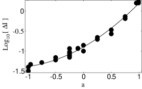
Figure 2: The (log of the) change of the potential’s maximum during the last radial orbit ($\log_{10}[\Delta I/\eta]$) versus $a$. The points show our $\Delta I$ for various cases with parameters $(p,e)$ close to those consistent with circular orbits (the boundary between stable and unstable orbits); these points were obtained from numerical solutions of the Teukolsky equation by Glampedakis and Kennefic, using the procedure described in Sec. II.4.1. For each $a$, solid circles show values of $\log_{10}[\Delta I/\eta]$ for several different values of $e$; that these points are all consistent with a single fit demonstrates that $\Delta I$is approximately independent of $e$. The solid curve is the quadratic fit Eq. (19). [In cases where insufficient data was present for extrapolation to the line $p=p_{s}(e,a)$, solid circles also indicate rough upper and lower limits expected of $\log_{10}[\Delta I/\eta]$.]

We need $\Delta I$ only for the particle’s last whirl. Since the maximum is extremely close to zero, the orbital parameters $(p,e,a)$ nearly satisfy a condition for the existence of (unstable) circular orbits $p=p_{s}(e,a)$ (see Appendix B). This curve also necessarily serves as the boundary between stable orbits and plunge. In the vicinity of this boundary line, $\Delta I$ is well-approximated by its nonzero values on the boundary. So for our computation we seek an expression $\Delta I(e,a)$.

In practice, from the values of $\Delta I$ at points near this boundary line, we extrapolate to estimate $\Delta I$ on the boundary surface itself. Figure 2 shows the results of our extrapolation.

One can argue that $\Delta I(p,e,a)$ on the last-stable-orbit boundary $p=p_{s}(e,a)$ should largely be independent of $e$ at moderate eccentricity . For this reason, Figure 2 shows results only as a function of one parameter ($a$). Numerical data over the range $e\in[0,0.5]$ support this conjecture. Therefore, so long as we avoid $e\approx 1$, where this conjecture has not yet been tested and likely fails, we can approximate $\Delta I/\eta$ by a function independent of $e$. Fitting a relatively simple function (exponential form in $a$, independent of $e$) to the data in Fig. 2 we find

$$\log_{10}\frac{\Delta I}{\eta}=-0.8972+0.7911a+0.3047a^{2}\;.$$ (19)

II.4.2 Estimating $I_{\text{ad,min}}$

To evaluate $I_{\text{ad,min}}$, we need no more than i) knowledge of the potential (which tells us $r_{\text{max}}$ as a function of $E$, $L$) and ii) knowledge of $dE/dt$, $dL/dt$ when the particles are in nearly-circular orbit near the hole.

In principle, we could approximate the latter by the appropriate values for an exactly circular (unstable) orbit. As a practical matter, comprehensive tabulation of the physically appropriate instantaneous $dE/dt$ and $dL/dt$ for all transitions of interest — namely, the values appropriate to a circular unstable orbit — proves time-consuming and technically challenging. Furthermore, because the crossing time depends only weakly (logarithmically) on $I$, and because exceedingly few particles will have $I\lesssim I_{\text{ad,min}}$, we only need $I_{\text{ad,min}}$ to order of magnitude.

Therefore, for practical purposes, when estimating $I_{\text{ad,min}}$ by way of Eq. (17) we will i) perform the computation for $dr_{\text{max}}/d\tau$ analytically in terms of $dE/dt$ and $dL/dt$, ii) simplify under the assumption $dE=\Omega dL$, which would be valid if we used the true forms for $dE/dt$ and $dL/dt$, and then iii) insert for $dL/dt$ the Peters-Mathews expression (an estimate obtained using linearized, quadrupolar emission from newtonian orbits) PetersMathewsRadiation

$$\frac{dL}{dt}\approx\eta\frac{32}{5}\frac{1}{p^{7/2}}(1-e^{2})^{3/2}\left[1+\frac{7}{8}e^{2}\right]\;.$$ (20)

II.4.3 Choosing $\delta r_{\text{ref}}$

To complete our procedure, we must define “the” transition duration. Unfortunately, because “the” transition from inspiral to plunge occurs at no definite location, has no well-defined start or finish, the transition duration remains a matter of convention . We shall adopt a convention motivated by a simple model of gravitational-wave data analysis.

The key feature of waves emitted during the transition is their considerable simplicity: they are emitted from a nearly-circular-equatorial orbit at $r_{\text{max}}$, and hence are characterized by the angular frequency $\Omega$ associated with circular orbits there. If we were to try to detect these gravitational waves — for simplicity, focusing on the dominant frequency component, $\omega=2\Omega$ — we would want to insure that our model $\phi=2\Omega t$ for the gravitational wave phase agrees, within $\pi$, with the true wave phase.

The true rate of change of orbital phase is

$$\frac{d\phi}{dt}(r,E,L)=\frac{g^{\phi\phi}L-g^{\phi t}E}{-g^{tt}E+g^{t\phi}L}\;,$$ (21)

where $g^{\alpha\beta}$ are known Kerr metric functions in Boyer-Lindquist coordinates, and $E$, $L$ are consistent with the circular orbit at $r=r_{\text{max}}$ (use standard expressions for $E$, $L$ appropriate to circular orbits, such as Eqs. (2.12) and (2.13) of Bardeen, Press, and Teukolsky CircularOrbits ). Demanding that the difference between the true angular phase and our fiducial reference $2\Omega t$ be no more than $\pi$ over the length of the transition, we find a constraint on the crossing duration $T_{c}$:

$$\pm 2\pi/4=\int_{-T_{c}/2}^{T_{c}/2}\left[\frac{d\phi}{dt}(r(t))-\frac{d\phi}{dt}(r_{\max})\right]dt.$$ (22)

When we insert $r(t)-r_{\max}=A\sinh\left[t/\tau_{o}\gamma\right]$ with $A=\sqrt{I}\tau_{o}$ [Eq. (7)] into the above, we find an expression we can invert for $\delta r_{\text{ref}}(\Delta I)$:

$$\pi/4\approx\left|\frac{d(d\phi/dt)}{dr}\right|\gamma\tau_{o}\sqrt{\delta r_{\text{ref}}^{2}+A^{2}}\approx\left|\frac{d(d\phi/dt)}{dr}\right|\gamma\tau_{o}\delta r_{\text{ref}}$$ (23)

[where the constant $A$ has been neglected in this expression, as it is always much smaller than $\delta r_{\text{ref}}$]. Solving for $\delta r_{\text{ref}}$, we obtain

$$\delta r_{\text{ref}}=\frac{\pi}{4\gamma\tau_{o}|d(d\phi/dt)/dr|}.$$ (24)

We will use this form even when it predicts $\delta r_{\text{ref}}=O(1)$ [in other words, when $\delta r_{\text{ref}}=O(M)$ when we convert to physical units]. Notice this $\delta r_{\text{ref}}$ is independent of mass ratio.

III Estimating the probability for LISA to observe a transition

We wish to estimate, for each choice of the supermassive hole’s angular momentum and distance from earth, and for each choice of test particle orbital parameters, the signal-to-noise ($S/N$) LISA would obtain from waves emitted during the transition. By combining this $S/N$ with the (poorly-known) statistics of black-hole inspirals, we can estimate the probability LISA will see a transition event (e.g., have $S/N>5$).

III.1 Estimating LISA’s signal to noise for a given transition

Since the transition waves are emitted by a circular orbit of frequency

$$f_{\text{orb}}=\Omega(r_{\text{max}})/2\pi M,$$ (25)

the gravitational waves will be at that frequency and its harmonics. For simplicity, assume that LISA detects only the strongest waves, the waves emitted from the second harmonic $f_{\text{tr}}=2f_{\text{orb}}$. These waves will last for an interval

$$\Delta t=N_{c}/f_{\text{orb}}(=MT_{c})\;.$$ (26)

We can approximate their characteristic rms (source-orientation-averaged) amplitude [following OT equation (4.7)] as a Peters-Mathews-style quadrapole term (averaged over all orientations) times a relativistic correction:

$$h^{\text{rms}}=\frac{8}{\sqrt{5}}\frac{M}{d}\eta\Omega(r_{\text{max}})^{2/3}\sqrt{\dot{\cal E}_{\infty,2}}\;.$$ (27)

Here $d$ is the distance to the source and $\dot{\cal E}_{\infty,2}$ is a relativistic correction factor defined explicitly in OT equation (2.3).

LISA has a spectral density of noise $S_{h}$ for waves incident on it with optimal propagation direction and polarization; it has spectral density $5S_{h}$ for typical directions and polarizations. Therefore, on average, LISA should accumulate a signal-to-noise from the transition event given by

$$\left(S/N\right)_{tr}=\frac{h^{\text{rms}}}{\sqrt{5S_{h}(f_{\text{tr}})/\Delta t}}\;.$$ (28)

Particularly special sources could have significantly higher $S/N$. For example, we can pick up an increase of $\sqrt{5}$ if the source is ideally positioned on the sky, and a similar increase if the source itself is optimally oriented. But overall, the above scheme suffices to estimate the signal-to-noise LISA would see from the transition between inspiral and plunge for any capture $m$ into $M$ with any specific source parameters (e.g., $e$, $a$) at any distance $d$.

Explicit expressions needed to compute LISA’s signal to noise for a given transition

To evaluate Eq. (28), we need in addition to $N_{c}$ and $\Omega$ [which enter into $S/N$ via $\delta t$ and $f_{\text{tr}}$] the LISA noise curve $S_{h}$ and the relativistic correction factor $\dot{\cal E}_{\infty,2}$. The LISA noise curve may be modeled by [OT equation (4.9)]

$$S_{h}(f) = \left[(4.6\times 10^{-21})^{2}+(3.5\times 10^{-26})^{2}\left(\frac{1\text{Hz}}{f}\right)^{4}\right.$$ (29)

$$\left.+(3.5\times 10^{-19})^{2}\left(\frac{f}{1\text{Hz}}\right)^{2}\right]\text{Hz}^{-1}\;.$$

The appropriate relativistic correction factor $\dot{\cal E}_{\infty,2}$ can in principle be extracted from simulations of waves emitted by particles in unstable circular orbits. As in practice the latter proves time-consuming to evaluate and tabulate for all possible eccentric orbits and for all $a$, for simplicity we will assume that the appropriate relativistic correction factor is i) fixed for all orbits close to a black hole of angular momentum $a$ and ii) given explicitly by the value appropriate to the innermost stable circular orbit (ISCO). This latter expression has been tabulated by Ori and Thorne (see the $\dot{\cal E}_{\infty,2}$ column in their Table II); we approximate their results by

$$\log_{10}\left(\dot{\cal E}_{\infty,2}\right)_{\text{OT}} \approx -0.0473+0.211x-0.053x^{2}$$ (30)

$$+0.034x^{3}+0.010x^{4}$$

where $x=\log_{10}(1-a)$.

Dominant terms in the signal-to-noise estimate

As written, the signal-to-noise estimate Eq. (28) disguises what kinds of effects predominantly influence it — for example, whether changes in the strength of radiation emitted prove more important or less than changes in the duration $T_{c}$ of the transition. To clarify the dominant contributions to our estimate, fix some $a$ and compare the signal-to-noise between two transitions ($1$,$2$) involving otherwise arbitrary parameters (e.g., $m$, $M$, $d$, $e$). Substituting expressions for $\Delta t$ [Eq. (26)], $h^{\text{rms}}$ [Eq. (27)], and $f_{\text{tr}}=2f_{\text{orb}}$ [Eq. (25)] into Eq. (28); assuming $\dot{\cal E}_{\infty,2}$ is a fixed function of $a$; and comparing the resulting $S/N$ at two sets of orbital parameters, we find

$$\frac{(S/N)_{2}}{(S/N)_{1}} = \frac{m_{2}}{m_{1}}\frac{d_{1}}{d_{2}}\sqrt{\frac{N_{c,2}}{N_{c,1}}}\left(\frac{\Omega_{1}}{\Omega_{2}}\right)^{1/6}$$ (31)

$$\times\sqrt{\frac{M_{1}S_{h}\left(\frac{\Omega_{2}}{\pi M_{2}}\right)}{M_{2}S_{h}\left(\frac{\Omega_{1}}{\pi M_{1}}\right)}}.$$

The first two terms reflect the natural $m/d$ scaling of emitted waves. The third term reflects the fact that more orbits around the hole during the transition mean more gravitational wave cycles seen by LISA. The fourth term, which combines the fact that gravitational waves emitted closer to the hole are stronger and yet last for less time, is to a good approximation constant. Finally, the last term reflects LISA’s sensitivity. The only term which depends explicitly on $M$ (ignoring the weak variation in $N_{c}$), this last term selects black hole masses which have their transition close to optimally positioned in the LISA band, or $M\approx\text{(few)}\times 10^{6}$. So long as the mass is so, this term varies comparatively little.

III.2 Method for estimating the probability of detecting some transition during LISA’s operation

Above we gave a procedure for computing the $S/N$ for any given source. But the sources which produce the strongest signals (inspirals very close by) are rare. Therefore, for any given $(S/N)_{o}$ we have a certain probability that, during the entire operation time $T_{L}$ of LISA, we detect no inspirals with $S/N>(S/N)_{o}$.

Since the relevant statistics for supermassive black holes and compact objects are poorly known, we will not attempt a detailed calculation that allows for all possible factors (e.g., source-orientation effects). Instead, for a first-pass estimate of the likelihood that LISA will see a transition, we will i) fix $M=10^{6}$, ii) approximate LISA’s noise curve as flat (in other words, ignore variations in $S/N$ due to the emitted radiation being slightly off LISA’s peak sensitivity), iii) ignore any orientation-related increase in the emissivity of the source or the sensitivity of LISA, iv) approximate $N_{c}$ as independent of $m$, v) further replace $N_{c}$ at each $a$ by some characteristic number of cycles (the precise value to be chosen later, when we understand how $N_{c}$ varies), and vi) assume all black holes have the same value of $a$ (again, to be chosen later). To be particularly explicit, we assume the $S/N$ varies with $m$, $d$, and $a$ in the following manner:

$$\left(\frac{S}{N}\right)(m,d,a) \approx \frac{m}{10M_{\odot}}\frac{1\text{Gpc}}{d}\left(\frac{S}{N}\right)_{\text{A}}$$ (32)

$$= K\frac{m}{d}\;.$$

Here $(S/N)_{A}\equiv(S/N)_{A}(10M_{\odot},1\text{Gpc},a)$ is a fiducial approximation to the signal to noise ratio for an inspiral with $m=10M_{\odot}$, $d=1\text{Gpc}$, and $a$.

Suppose we have a discrete family of possible compact objects of masses $m_{k}$ with rates (per galaxy containing a $10^{6}M_{\odot}$ hole) $r_{k}$; suppose the number density of galaxies containing a $10^{6}M_{\odot}$ hole is $\rho_{g}$. Subdividing the universe into cubes of cell size $\Delta r$, we find the probability a given cell has an inspiral of mass $m_{k}$ into a $10^{6}M_{\odot}$ hole at some time during the lifetime $T_{L}$ of LISA is $p_{k}=\rho_{g}r_{k}T_{L}\Delta r^{3}$. Suppose we’re concerned with a threshold $S/N$ level $S/N=s_{o}$. At such a level we could see a source of mass $m_{k}$ out to a distance $d_{k}=Km_{k}/s_{o}$. If no inspirals have $S/N>s_{o}$, then for every cell in range, we have no inspirals of any mass type. Therefore, the probability that no inspirals occur with $S/N<s_{o}$ is

$$P(\text{no }S/N>s_{o}) = \prod_{k}(1-p_{k})^{4\pi d_{k}^{3}/3\Delta r^{3}}$$ (33)

$$\approx \exp\left[-\frac{4\pi R_{\text{net}}T_{L}}{3}\frac{K^{3}\left<m^{3}\right>}{s_{o}^{3}}\right]$$

where in the last line we use $p_{k}\ll 1$, $R_{\text{net}}\equiv\sum\rho_{g}r_{k}$ (the net event rate per unit volume for all inspirals), and $<m^{3}>\equiv\sum\rho_{g}r_{k}m^{3}/R_{\text{net}}$ (the mean cubed mass of inspiralling bodies, where weights are by event rate). Note that $4\pi K^{3}\left<m^{3}\right>/(3s_{o}^{3})$ is the volume of space in which an inspiral involving a mass $\left<m^{3}\right>^{1/3}$ can be seen with a signal-to-noise ratio $>s_{o}$. Necessarily, the probability that some source has $S/N>s_{o}$ is $P(\text{some }S/N>s_{o})=1-P(\text{no }S/N>s_{o})$

We can reorganize this expression to tell us, for a given probability $P_{\text{no}}$, at what $S/N$ we will have a probability $P_{\text{no}}$ of having no signals of stronger strength:

$$\left(\frac{S}{N}\right)_{\text{no}}(P_{\text{no}}) \equiv \frac{\left<m^{3}\right>^{1/3}}{10M_{\odot}}\frac{1\text{Gpc}}{\left(\frac{4\pi}{3}R_{net}T_{L}\right)^{-1/3}}\frac{1}{[\ln(1/P_{\text{no}})]^{1/3}}$$ (34)

$$\times\left(\frac{S}{N}\right)_{A}\;.$$

III.3 Probability of detecting a transition during LISA’s operation

The $S/N$ threshold [Eq. (34)] depends very sensitively (through $\left<m^{3}\right>^{1/3}$) on low-probability high-mass inspirals. By way of illustration, a family of $0.6M_{\odot}$ white dwarfs inspiralling with rate $R$ and a black hole family of mass $30M_{\odot}$ and rate $10^{-4}R$ contribute in similar proportions to $\left<m^{3}\right>^{1/3}$. At present, the astrophysical community lacks sufficiently understanding of the high-mass tail to be able to reliably compute $\left<m^{3}\right>^{1/3}$. Therefore, we will neglect such objects and focus on the slightly-better understood problem of capture of conventional compact objects. Doing so, we will underestimate the true $(S/N)_{\text{no}}$.

Even disregarding the high-mass holes, event rates for capture InspiralRatesFreitag ; InspiralRatesRees remain very loosely determined, ranging from rates of $\sim 2\times 10^{-6}$/yr/galaxy to $\sim 10^{-4}$/yr/galaxy. We take two cases as characteristic:

• Freitag (F) Based on astrophysical discussion by Miralda-Escude and Gould InspiralRates3 , Freitag allows for three species: white dwarfs ($m_{\text{WD}}=0.6M_{\odot}$, $r_{WD}\sim 10^{-5}$/yr); neutron stars ($m_{\text{NS}}=1.4M_{\odot}$, $r_{NS}\sim 2\times 10^{-6}$/yr); and black holes ($m_{\text{BH}}=7M_{\odot}$, $r_{BH}\sim 10^{-6}$/yr). In this case, the net event rate $R_{\text{net}}$ is dominated by low-mass WD inspirals, but black holes dominate the events seen by LISA. Using a LISA lifetime $T_{L}=3\text{ yr}$ and (based on Sigurdsson and Rees’s estimate that the density of $10^{6}M_{\odot}$ holes at their cores is around the density of spirals, since spirals have low mass and ellipticals high mass supermassive holes InspiralRatesRees ) $\rho_{g}\sim 0.003/\text{Mpc}^{3}$, we find

  $$\left(\frac{S}{N}\right)_{\text{no,F}} = 2.67\left(\frac{\ln(2)}{\ln(1/P_{\text{no}})}\right)^{1/3}$$

  $$\times\left(\frac{S}{N}\right)_{A}\left(10M_{\odot},1\text{Gpc}\right).$$

• Sigurdsson and Rees (SR) They consider two types of galaxies — spirals and dwarf ellipticals — but only the latter leads to significant event rates. In that case, they uses the following masses and rates for the three species: WD ($m_{\text{WD}}=0.6M_{\odot}$, $r_{WD}\sim 3\times 10^{-8}$/yr); NS ($m_{\text{NS}}=1.4M_{\odot}$, $r_{NS}\sim 10^{-7}$/yr); and BH ($m_{\text{BH}}=5M_{\odot}$, $r_{BH}\sim 10^{-6}$/yr). (For black holes, these authors provide only an off-the-cuff estimate; we have taken some liberty in interpreting it, choosing a mildly optimistic characteristic black hole mass.) Again using $T_{L}=3\text{ yr}$ and $\rho_{g}=0.003/\text{Mpc}^{3}$, we find

  $$\left(\frac{S}{N}\right)_{\text{no,SR}} = 1.90\left(\frac{\ln(2)}{\ln(1/P_{\text{no}})}\right)^{1/3}$$

  $$\times\left(\frac{S}{N}\right)_{A}\left(10M_{\odot},1\text{Gpc}\right).$$

In performing both calculations, we use Sigurdsson and Rees’s estimate that the density of galaxies with (spirals have low-mass holes; ellipticals and others tend to have more), so $\rho_{g}\sim 0.003/\text{Mpc}^{3}$. Also, we use a LISA lifetime $T_{L}=3$ yr.

In sum, we suspect that on astrophysical grounds we will have a 50% chance of seeing no source with $S/N$ roughly greater than

$$\left(\frac{S}{N}\right)_{\text{no,guess}}\approx 2.5\times\left(\frac{S}{N}\right)_{A}\;,$$ (35)

where the $(S/N)_{\text{A}}$ will chosen to be the most reasonable $S/N$ over all orbital parameters ($e$) and black hole spins ($a$), given the fiducial parameters $d=1\text{Gpc}$, $m=10M_{\odot}$, and $M=10^{6}M_{\odot}$.

IV Schwarzchild Supermassive black hole (SMBH)

To illustrate this scheme in a case where all terms are algebraically tractable, we discuss the range of probable transition durations when the capturing hole has no angular momentum (Schwarzchild).

IV.1 Choosing parameters

Rather than using $E,L$ to characterize the orbit, when the orbit is confined in radius between two turning points (i.e. when it is bound), it is far simpler to characterize the potential $V=-(dr/d\tau)^{2}$ by the location of its 3 roots, $r_{\pm},\bar{r}$, where $r_{\pm}$ are the inner and outer turning points of the bound orbit and $\bar{r}$ is the innermost root:

$$\left(\frac{dr}{d\tau}\right)^{2} = -V=\frac{1-E^{2}}{r^{3}}\left(r_{+}-r\right)\left(r-r_{-}\right)\left(r-\bar{r}\right)$$ (36)

$$= E^{2}-\left(1-\frac{2}{r}\right)\left(1+\frac{L^{2}}{r^{2}}\right)$$

Since we have only two free parameters, the three roots are not independent; they satisfy a self-consistency polynomial. For this reason, we introduce $p,e$ — parameters analogous to semi-latus rectum and eccentricity in classical mechanics. Employing a consistency relation [generally Eq. (59) of Appendix B] to set $\bar{r}$, we find

$$r_{\pm}\equiv\frac{p}{1\mp e}\/,\qquad\bar{r}=\frac{2p}{p-4}\/,$$ (37)

$$E^{2}=\frac{\left(p-2-2e\right)\left(p-2+2e\right)}{p\left(p-3-e^{2}\right)}\/,\qquad L^{2}=\frac{p^{2}M^{2}}{p-3-e^{2}}.$$ (38)

These $p,e$ parameters have the notable advantage that bound orbits (orbits that cannot escape to infinity) and non-plunging orbits (orbits which avoid the central black hole) are easy to describe: bound orbits have $e\in[0,1]$, while non-plunging orbits have $0<r_{-}-\bar{r}=p(p-6-2e)/[(1+e)(p-4)]$, or

$$z=p-6-2e>0.$$ (39)

As one approaches the transition, the maximum of the potential $V$ decreases, $r_{-}$ approaches $\bar{r}$, and $z$ approaches $0$. We can equivalently specify the location $r$ of a transition by only one of $p$ or $e$, with the other determined by $z=0$. I will typically use $e$. For example, a transition of eccentricity $e$ occurs at radius $r=r_{-}=\bar{r}=2(3+e)/(1+e)$.

The parameters $p$, $e$ used here are identical to those used the Teukolsky-equation-based inspiral literature CKP ; Dan . For example, the above discussion mirrors that in Cutler, Kennefick, and Poisson CKP between their equations (2.4) and (2.8), with the change of notation $r_{1}\rightarrow r_{-}$, $r_{2}\rightarrow r_{+}$ and $r_{3}\rightarrow\bar{r}$.

IV.2 Dependence of Transition Parameters on Eccentricity

We know the potential [Eq. (36)]; hence we find that when $r_{-}=\bar{r}$ (=the transition radius) we have

$$V^{\prime\prime}=-(1-E^{2})2\frac{r_{+}-r_{-}}{r_{-}^{3}}$$ (40)

and therefore, substituting $r_{\pm}$ and $E$ from Eqs. (37), (38) into $\tau_{o}=(V^{\prime\prime}/2)^{-1/2}$ we find

$$\tau_{o}=(3+e)\sqrt{\frac{2(9-e^{2})}{e(1+e)^{3}}}.$$ (41)

Similarly, substituting $r=r_{-}$ into $\gamma=-g^{tt}E$ gives us the characteristic time required to make the transition:

$$\gamma\tau_{o}=\frac{2(3+e)^{2}}{\sqrt{e(1+e)^{3}}}$$ (42)

Since $d\phi/dt=g^{\phi\phi}L/(-g^{tt}E)=L/r^{2}(1-2/r)E$, we find

$$\left(\frac{d}{dr}\frac{d\phi}{dt}\right)_{r=r_{\text{max}}} = \frac{2(r_{\text{max}}-3)}{r_{\text{max}}^{5/2}(r_{\text{max}}-2)}\;,$$ (43)

when $E$, $L$ are consistent with a circular orbit at $r=r_{\text{max}}$. Using the above and Eq. (24), we conclude that for moderate eccentricity the natural “transition extent” $\delta r_{\text{ref}}$ is

$$\delta r_{\text{ref}}\approx\pi\frac{\sqrt{2e(3+e)}}{(1+e)(3-e)}.$$ (44)

This scale naturally varies with the scale of the potential (namely, $\delta r_{\text{ref}}\propto 1/\sqrt{V^{\prime\prime}}$) as $e\rightarrow 0$.

Further straightforward computations using the potential [Eq. (36)] reveal how $r_{\text{max}}$ varies due to loss of $E$ and $L$ via wave emission when the particle is nearly in a circular orbit (so $dE\approx\Omega dL$):

$$\frac{dr_{\text{max}}}{dt}=\frac{dL}{dt}2\frac{(r_{\text{max}}-3)^{3/2}}{r_{\text{max}}-6}\;.$$

We therefore can express $I_{\text{ad,min}}$ in terms of (tabulated) known radiation-reaction angular momentum fluxes $\left<dL/dt\right>$:

$$I_{\text{ad,min}}=\left(\frac{dL}{dt}\right)^{2}\frac{(3-e)^{2}(3+e)}{2e^{2}(1+e)}\;.$$ (45)

To obtain a rough approximation of $I_{\text{ad,min}}$, rather than use the true $dL/dt$ appropriate to circular orbits, we approximate $dL/dt$ by the Peters-Mathews expression [Eq. (20)].

Our scheme ceases to apply when the eccentricity is below $e_{\text{ad}}$ defined by $\Delta I=I_{\text{max}}(e_{\text{ad}})$ [Eq. (16)]. In the special case of $a=0$, where $p_{s}=6+2e$, the definition of $I_{\text{max}}$ [Eq. (61)] reduces to

$$I_{\text{max}}=\frac{32}{27}\frac{e^{3}}{(9-e^{2})(1+e)}\;.$$ (46)

IV.3 Transition duration

With all the necessary elements assembled, we can apply our program [Eqs. (9), (11), (18)] to estimate the distribution in number of orbital cycles $N_{c}\equiv T_{c}\Omega/2\pi$ we expect when a particle spirals into a nonspinning black hole at some fixed, known eccentricity $e$.

The results for $\eta=10^{-5}$ are shown in Fig. 3.

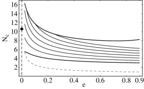
Figure 3: Plots of various predictions for the expected number of angular cycles ($N_{c}$) versus eccentricity ($e$) for a transition from inspiral to plunge with $\eta=10^{-5}$. The top solid curve is the number of cycles when $T_{c}=T_{c,\text{ad}}$ [Eq. (18)], an estimate of the longest possible (adiabatic) transition duration. The bottom solid curve is the number of cycles when $T_{c}=T_{c,-}$ [Eq. (9)]. The 6 curves in between are the number of cycles when $T_{c}=T_{c,1},\ldots T_{c,6}$ [Eq. (11)]; as only a fraction $\approx 10^{-1},\ldots,10^{-6}$ of inspirals can have durations above these curves (respectively), they illustrate how few particles have durations significantly differing from $T_{c,-}$. The dot indicates the Ori-Thorne (OT) prediction for circular equatorial inspiral. The dashed curve is a characteristic-scale-based prediction based on $T_{c}=4\gamma\tau_{o}$, used to illustrate the significance of the “logarithmic correction.” The plot starts at $e=e_{\text{ad}}\approx 0.0215$, at which point $\Delta I=I_{\text{max}}$.

When our adiabatic approximation applies, we find that to a good approximation (within around 1 cycle) most transitions should have duration close to the shortest transition duration $N_{c,\text{ad}}=T_{c,\text{ad}}\Omega/2\pi\in[3,5]$. In particular, within the region $e>e_{\text{ad}}$ where our adiabatic approximation applies, almost all transitions will last for less than the Ori-Thorne (OT) circular duration; most will last for substiantially less. At low eccentricity, most transitions seem to approach a result somewhat different than the OT circular estimate. Since OT use a different convention for $\delta r$ and since significant changes could still occur in the fundamentally nonadiabatic region between $e=0$ and $e=e_{\text{ad}}$, we do not find the discrepancy troubling.

In the above, we show results for only $\eta=10^{-5}$ (say, for $m=10M_{\odot}$ and $M=10^{6}$). As the variation of the duration with $\eta$ is weak — we find $H(\eta_{o}=10^{-5})\in[0.1,0.4]$) [Eq. (14)] — even substantially different test particle masses (e.g., $m\in[0.1,30]M_{\odot}$ with $M=10^{6}$) lead to results of the form above, scaled up or down by a factor $\lesssim 2$.

IV.4 Prospects for LISA detecting a given transition

As discussed in Sec. III, we can estimate the signal-to-noise ratio for a given transition using Eq. (28). For the standard case of a $10M_{\odot}$ particle falling into a $M=10^{6}M_{\odot}$, application of that formula reveals no higher $S/N$ than that predicted by Ori and Thorne; moreover, barring astrophysically unlikely masses, all transitions have too low a $S/N$ to be detected. [See Fig. 7 below for details.] For example, if an inspiral of mass $m$ into a $10^{6}M_{\odot}$ hole occurs at the fiducial distance $1$ Gpc with $e=1/3$, we have a 90% chance that $S/N\in[0.91,1.01](m/10M_{\odot})$.

The results for $S/N$ can be well-approximated by way of Eq. (31) and a comparison with Ori and Thorne’s results for circular inspiral. (See Appendix C for a summary of OT results). Specifically, using the fiducial case of $10M_{\odot}$ on $10^{6}M_{\odot}$ at $1$ Gpc, for which we have $(S/N)_{OT}=1.6$ and $N_{c,OT}=10.5$, we find the general $S/N$ for captures by a $M=10^{6}M_{\odot}$ hole to be about

$$(S/N) \approx 1.6\times\sqrt{\frac{N_{c}}{10.5}}\times\frac{m}{10M_{\odot}}\frac{1\text{Gpc}}{d}\;.$$

V Kerr SMBH

The Kerr case follows similarly, save with an additional parameter ($a$).

V.1 Parameterizing Orbits, Potential

As before, it is simplest to characterize the potential by its three roots $r_{\pm}=p/(1\mp e)$, $\bar{r}$:

$$\left(\frac{dr}{d\tau}\right)^{2}=-V=\frac{1-E^{2}}{r^{3}}\left(r_{+}-r\right)\left(r-r_{-}\right)\left(r-\bar{r}\right).$$ (47)

And as before we can define $r_{\pm}=p/(1\mp e)$; as before, we find a self-consistency relation $P(p,e,a,\bar{r})$ [Eq. (59)], permitting us to solve for $\bar{r}(p,e,a)$. As before, we can characterize the proximity to the last-stable surface by way of the separation between the two innermost roots ($r_{-}-\bar{r}$). Finally, as before, for each fixed black hole ($a=$const) and each particle exactly on the transition line from orbit to plunge, the particle can have $e\in[0,1)$; its $p$ will be constrained by the analogue of the Schwarzchild $p=6+2e$: the self-consistency relation Eq. (60), which implicitly defines $p_{s}(e,a)$ such that $\bar{r}(p_{s},e,a)=p_{s}/(1+e)$.

V.2 Dependence of transition parameters on $e$,$p$

Since the potential has the same structure as before, the same general expression Eq. (40) applies, with $E$ now determined by expressions in Appendix B. By explicitly differentiating the potential [Eq. (2)], inserting the definitions $r_{\pm}=p/(1\mp e)$, and demanding the inner turning point is a maximum (so $\bar{r}=r_{-}=p/(1+e)$), we find

$$V^{\prime\prime}=-8e\frac{(1+e)^{3}}{(3-e)p_{s}^{3}}$$ (48)

and therefore know $\tau_{o}=(V^{\prime\prime}/2)^{-1/2}$ in terms of $p,e$ at the transition.

The $\gamma$ factor follows from inserting $r=p/(1+e)$ into the usual expression for $dt/d\tau$:

$$\gamma\equiv\frac{dt}{d\tau}=-g^{tt}E+g^{t\phi}L$$ (49)

where $g^{tt}$ and $g^{t\phi}$ are known Kerr metric coefficients. Here, $E$ and $L$ are evaluated using the expressions (57) and (58) discussed in Appendix B, with $\bar{r}=p_{s}/(1+e)$.

We obtain the transition extent $\delta r_{\text{ref}}$ with the usual Eq. (24). This requires $\gamma$ [Eq. (49), above], $\tau_{o}$ (also above), and $d(d\phi/dt)/dr$ [Eq. (21)].

Finally, as in the Schwarzchild case we estimate $I_{\text{ad,min}}$ [Eq. (17)] and thus $T_{c,\text{ad}}$ [Eq. (18)] via i) expressing $dr_{\text{max}}/d\tau$ in terms of $dL/dt$ using explicit expressions for $r_{\text{max}}(E,L)$ and $dE=\Omega dL$, giving

$$\frac{dr_{\text{max}}}{dt}=\frac{dL}{dt}\left.\frac{2r(2a\sqrt{r}+r^{2}-3r)^{3/2}}{(r^{3/2}+a)(r^{2}-6r+8a\sqrt{r}-3a^{2})}\right._{r=r_{\text{max}}}\;,$$ (50)

(where we have used the orbital parameters $E$,$L$ consistent with a circular orbit at $r=r_{\text{max}}$ CircularOrbits ); then ii) using the Peters-Mathews expressions for $dL/dt$ [Eq. (20)] to construct an approximate expression for $dr_{\text{max}}/dt$, which we then iii) insert in Eq. (17) to estimate the boundary between adiabatic and nonadiabatic transitions.

V.3 Transition duration

Combining these together, we can deduce the range of plausible transition durations for a test particle of eccentricity $e$ falling into a hole of angular momentum $a$, measured as number of orbital cycles $N_{c}(e,a)=T_{c}\Omega/2\pi$. Plots of the number of cycles appropriate to $T_{c}=T_{c-}$ [Eq. (9)], to $T_{c}=T_{c,\text{ad}}$ [Eq. (18)], and to $T_{c}=T_{c,1}$ [Eq. (11)] appear in Figs. 4, 5, and 6, respectively.

These plots all assume a fiducial source ($10M_{\odot}$ on $10^{6}M_{\odot}$). In these plots, we truncate the range of $e$, $a$ allowed because, i) we need $e$ larger than $e_{\text{ad}}$ [Eq. (16)]; and ii) realistic astrophysical black holes have $a\leq 0.998$ LargestA . Also, in these plots, we do not extend to $e\approx 1$ because we do not have data for $I$ in this region, nor do we expect our estimate of $\Delta I$ [Fig. 2] to be reliable in this extreme.

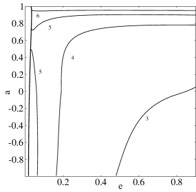
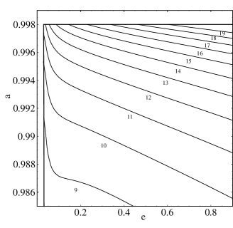
Figure 4: These two plots illustrate the shortest possible number of cycles $N_{c}=\Omega T_{c-}/2\pi$ [Eq. (9)] a transition could last, versus eccentricity ($e$) and black hole angular momentum $(a)$ for the fiducial source ($10M_{\odot}$ into $10^{6}M_{\odot}$). In both plots, contours are cut off, and bounding curves appear (shown heavy solid), when $\Delta I=I_{\text{ad,min}}$ and when $a=0.998$.

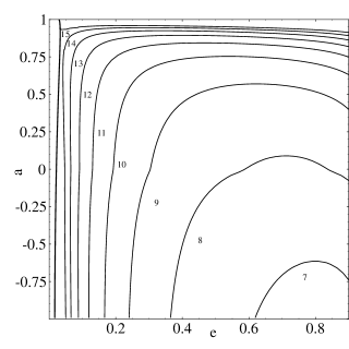
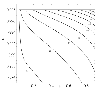
Figure 5: These two plots illustrate the longest possible number of cycles an (adiabatic) transition could last $N_{c}=\Omega T_{c,\text{ad}}/2\pi$ [Eq. (18)], versus eccentricity ($e$) and black hole angular momentum ($a$) for the fiducial source ($10M_{\odot}$ into $10^{6}M_{\odot}$). Transitions of such long duration are extremely unlikely unless $e\approx e_{\text{ad}}$ [see Eq. (16), (10)]. In both plots, contours are cut off, and bounding curves appear (shown heavy solid), when $\Delta I=I_{\text{ad,min}}$ and when $a=0.998$.

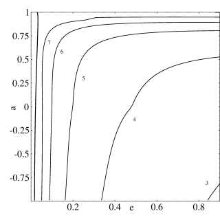
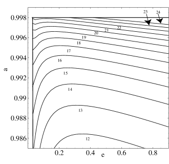
Figure 6: These two plots illustrate $N_{c}=\Omega T_{c,1}/2\pi$ versus $e$ and $a$ for the fiducial case. When the results of Fig. 5 are appreciably larger than these — that is, everywhere except near the left boundary $e=e_{\text{ad}}$ — $\sim$ 90% of transitions with orbital parameters $e$, $a$ will take less than the number of cycles shown in this plot to traverse the transition region.

At each $a$, we see behavior largely similar to the Schwarzchild results discussed in Sec. IV: i) almost all transitions take less time than the Ori-Thorne result for $e=0$; ii) as we increase the eccentricity, the transition duration decreases; and iii) since $T_{c,1}\approx T_{c,-}$ (compare Figs. 4 and 6), most transitions last close to the shortest-possible transition duration.

V.4 Prospects for LISA detecting a given transition

As in the Schwarzchild case, since eccentric usually transitions last for fewer angular cycles than their circular analogues, they are less detectable as well. Thus, in the fiducial case of captures of a $10M_{\odot}$ hole by a $10^{6}M_{\odot}$ hole, the data from Ori-Thorne Table II provides an upper bound on the S/N seen by LISA (shown in Fig. 7). Since this bound is small, we have little chance of seeing any given transition.

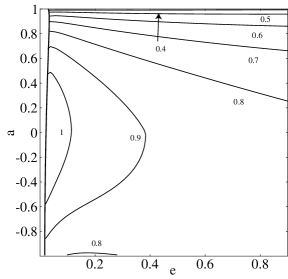
Figure 7: This plot illustrates $S/N$ [Eq. (28)], given a fiducial source ($10M_{\odot}$ into $10^{6}M_{\odot}$, at $1\text{Gpc}$) given that the black hole has angular momentum $a$, the transition occurs at eccentricity $e$, and given the transition takes the shortest possible time (or $T_{c}=T_{c,-}$) [Eq. (9)]. As argued in the text, this time (and thus this $S/N$) will be to a good approximation characteristic of all transitions with those interaction parameters.

One should notice, however, that the distribution of $S/N$ with orbital parameters is very flat and not much below $1$. Therefore, only a modest improvement in LISA’s noise spectrum $S_{h}$ could render most (measured by volume of parameter space) of the transitions detectable.

V.5 On probability of detection

Because LISA at present has so poor prospects for detecting the “fiducial” source ($m=10M_{\odot}$ at $1$Gpc), it has a poor chance of seeing any source at all. Even assuming all LISA sources had orbital parameters chosen to give the longest-plausible transition length (the OT circular inspiral duration, which has $S/N_{A}\lesssim 1.6$), by the estimate of Eq. (35) we expect we have a $\sim$50% chance of no signal with $S/N\gtrsim 4$ being present in the datastream. With more realistic orbital parameters, we would expect a $\sim$50% chance of no signal $\gtrsim 2.3$. In other words, LISA has a good to excellent chance of not seeing any transitions from inspiral to plunge in its lifetime.

A modest improvement in LISA’s noise curve, however, would make a few circular (and to a lesser degree eccentric) transitions from inspiral to plunge detectable.

VI Summary

This paper has introduced a framework (depending on observational or other conventions) that extends the Ori-Thorne prediction for the transition duration from inspiral to plunge to include eccentric orbits. While the framework and applications contain many oversimplifications — most notably, the fit to $\Delta I(e,a)$ and and the lack of a physically meaningful convention for $\delta r_{\text{ref}}$ — the essential physics should be captured by Sec. II.

This paper then applies that framework to probable LISA sources to suggest that, because an eccentric transition is generally only slightly briefer than a circular one, LISA should have only slightly worse prospects to resolve the transition from inspiral to plunge for eccentric orbits than for circular ones. While the prospects for detecting circular (and hence eccentric) transitions with LISA are not good, they are not necessarily bad: modest changes to the LISA noise floor could render a signal marginally detectable. Therefore, more detailed investigations could be of use.

Potentially, we could use other portions of orbits that pass close to the hole — for example, the previous few “bounces” off the inner portion of the radial potential — as probes of the strong-field metric. Analyzed separately (using the same $\Delta I$ framework) each of these “bounces” should provide in itself at best of order the same S/N as the transition. If the source has already been detected with good confidence, we should be able to coherently integrate over many such bounces and build up excellent $S/N$.

Finally, we could hope that eccentric inclined orbits might, by some happenstance of parameters, admit a regime of significantly longer transition times. The prospect seems unlikely, but the author may address it in a future paper.

Appendix A Evolution of the maximum

As the conserved constants $E$, $L$ evolve, the height of any local maximum in the potential $V$ [Eq. (1)] will similarly evolve. Because we are at a local maximum, we can find a simple expression for the rate of change of the value of the potential at that local maximum:

$$V_{\max}(E,L)=V(r_{\max}(E,L),E,L)$$ (51)

(where $r_{\max}$, the location of the potential’s local maximum, is a solution to $dV/dr=0$). In general, to order of magnitude, we expect it goes as $\sim V/\tau_{\text{gw}}$ for $\tau_{\text{gw}}$ the gravitational wave timescale $\tau_{\text{gw}}\sim E/\dot{E}\sim L/\dot{L}$. But when the particle is nearly on a circular orbit, then the source of radiation nearly satisfies helical symmetry and therefore $dE\approx\Omega dL$ for $\Omega$ the angular frequency of the circular orbit. And in these special conditions $V$ changes even more slowly than we would normally expect.

To be explicit, we evaluate $dV_{\max}/dt$, which (because we are at a maximum) we can generally express as follows:

$$\frac{dV_{\max}}{dt}=\frac{\partial V}{\partial L}\left[\frac{dL}{dt}+\frac{dE}{dt}\frac{\partial V/\partial E}{\partial V/\partial L}\right]_{r=r_{\max}}\;.$$ (52)

We can most transparently prove the necessary result by rewriting the potential $V$ more abstractly than the standard form of Eq. (2). Recall one derives the radial potential from the constancy of the test-particle’s rest mass [e.g., $g^{ab}p_{a}p_{b}=-m^{2}$]. Since the Kerr metric in boyer-lindquist coordinates has form $g_{ab}=g_{tt}dt^{2}+2g_{t\phi}dtd\phi+g_{\phi\phi}d\phi^{2}+g_{rr}dr^{2}+g_{\theta\theta}d\theta^{2}$, by employing the definitions of $E$ and $L$ (e.g., $-p_{t}\equiv$ energy) and the existence of an equatorial orbit, one obtains the (first integral of the) radial geodesic equation Eq. (1) with $V=(1+E^{2}g^{tt}+L^{2}g^{\phi\phi}-2ELg^{t\phi})/g_{rr}$. One can similarly show, by employing the definitions of the “raised” components (e.g., $p^{t}\equiv mdt/d\tau$ for $\tau$ proper time), that $d\phi/dt=(g^{\phi\phi}L-g^{t\phi}E)/(-g^{tt}E+g^{t\phi}L)$ and $dt/d\tau=-g_{rr}\partial V/\partial E$. Using these expressions in Eq. (52), we conclude that

$$\frac{dV_{\max}}{dt}=-\frac{dt/d\tau}{g_{rr}}\left[\frac{dL}{dt}-\frac{dE}{dt}\frac{1}{d\phi/dt}\right]_{r=r_{\max}}.$$ (53)

When the potential admits a nearly-circular orbit (angular frequency $\Omega=d\phi/dt$) near the local maximum, we have $dE\approx\Omega dL$ in the emitted radiation and therefore $dV_{\text{max}}/dt$ is smaller than normal. [Similar arguments apply to the minimum, and prove that stable circular orbits evolve to stable circular orbits.]

Appendix B Kerr Parameters and Constraints

In the Teukolsky-equation-based inspiral literature CKP ; Dan , when the orbit is bound (=does not fall into hole or escape to infinity) it is characterized not by physical parameters ($E$,$L$,$a$) but by the location of its radial turning points ($r_{\pm}$) and the remaining root of its potential ($\bar{r}$):

$$V = \frac{E^{2}-1}{r^{3}}\left(r_{+}-r\right)\left(r-r_{-}\right)\left(r-\bar{r}\right)$$ (55)

$$= -\left(E^{2}-1\right)-\frac{2}{r}+\frac{\left[L^{2}-a^{2}\left(E^{2}-1\right)\right]}{r^{2}}$$

$$-\frac{2\left(L-aE\right)^{2}}{r^{3}}$$

To further simplify the algebra involved, one replaces $r_{\pm}$ by a parameterization analogous to classical mechanics (semi-latus rectum and eccentricity):

$$r_{\pm}=\frac{p}{1\mp e}$$ (56)

(with $p$,$e$ both real, positive). After replacing $r_{\pm}$ by $p,e$ using $r_{\pm}=p/(1\mp e)$, we find the following explicit forms for $E,L$ in general: (specify retrograde orbits by a negative $a$ sign)

$$E = \sqrt{1-\frac{\left(1-e^{2}\right)}{2p+\left(1-e^{2}\right)\bar{r}}}$$ (57)

$$L = \left[\text{sign}(a)\frac{p\sqrt{\bar{r}}}{\sqrt{2p+\left(1-e^{2}\right)\bar{r}}}+aE\right]$$ (58)

The parameters $p,e,\bar{r}$, however, are not fully independent. The coefficients of $V\left(r\right)$ satisfy a polynomial equation when the coefficients are expressed in terms of $L,E,a$; the coefficients must satisfy the same polynomial when the coefficients are written using $r_{\pm},\bar{r}$. Re-expressing that polynomial in terms of $p,e$, we find

$$0 = p^{2}\left[p\left(\bar{r}-2\right)-4\bar{r}\right]^{2}+a^{4}\left[p+\left(1-e^{2}\right)\bar{r}\right]^{2}$$ (59)

$$-2a^{2}p\left\{4\left(1-e^{2}\right)\bar{r}^{2}+2p^{2}\left(2+\bar{r}\right)\right.$$

$$+p\bar{r}\left.\left[8+\left(\bar{r}-2\right)\left(1-e^{2}\right)\right]\right\}$$

As a practical matter, we usually specify a particle by ($p$,$e$,$a$) and then solve for $\bar{r}$ and hence all other orbital parameters.

B.1 Separatrix

The transition from stable to unstable occurs when $\bar{r}=r_{-}=p/(1+e)$. We can attempt to express this relation in terms of the usual orbital parameters ($p$,$e$,$a$). Substituting in the above polynomial [Eq. (59)], we get

$$0= p_{s}^{2}\left(p_{s}-6-2e\right)^{2}+a^{4}\left(e-3\right)^{2}\left(1+e\right)^{2}$$ (60)

$$-2a^{2}\left(1+e\right)p_{s}\left[14+2e^{2}+p_{s}\left(3-e\right)\right]$$

where $p=p_{s}(e,a)$, defined by (appropriate solutions to) the above relation, determines the separatrix between stable and unstable geodesic orbits.

B.2 Minimum of potential

At the transition from stable to unstable orbits, the maximum of the potential is at $r_{-}=\bar{r}=p_{s}/(1+e)$. Therefore, by symbolically differentiating Eq. (55), we find $r_{\min}=3p_{s}/(3-e)$. Inserting this expression into $V$ and noting $V(r_{\max})=0$, we find $I_{\max}\equiv V(r_{\max})-V(r_{\min})$:

$$I_{max}=\left(\frac{4e}{3}\right)^{3}\frac{1}{(3-e)(1+e)p_{s}}$$ (61)

Appendix C Results from Ori and Thorne

So that the reader can more easily compare our estimates against those of Ori and Thorne, we provide approximations to their results.

In Ori and Thorne’s Table II, they tabulate $S/N$ and $N_{c}$ for $10M_{\odot}$ on $10^{6}M_{\odot}$, using fiducial distance $1$ Gpc to set the amplitude scale. [In this table, OT list the number of quadrupolar gravitational wave cycles $N_{\text{cyc}}=2N_{c}$.] We can approximate their results by the two functions

$$\log_{10}N_{c,\text{OT}} \approx 0.92+0.110x+0.0478x^{2}\;,\quad a\in[0.9,0.99]$$ (62)

$$\approx 1.03+0.073x+0.138x^{2}\;,a<0.9$$

and

$$\log_{10} \left(\frac{S}{N}\right)_{\text{OT}} \times 10^{-22}$$ (63)

$$\approx 0.3156+0.3193x+0.0451x^{2}\;,\quad{a\in[0.8,0.99]}$$

$$\approx 0.191-0.226x-0.448x^{2}\;,{a<0.8}$$

where $x\equiv\log_{10}(1-a)$.

- (1) F. D. Ryan, Phys. Rev. D. 56 (4) 1845
- (2) A. Buonanno, Y. Chen, M. Vallisneri, gr-qc/0205122
- (3) A. Buonanno and T. Damour, Phys. Rev. D 60, 023517 (1999)
- (4) L.E. Kidder, C.M. Will, and A.G. Wiseman, Phys. Rev. D 47 3281 (1993)
- (5) L. Lehner, CQG 18 (2001) R25
- (6) For LISA information, see http://lisa.jpl.nasa.gov
- (7) S. Detweiler and B. Whiting, gr-qc/0202086; Y. Mino, H. Nakano, and M Sasaki, gr-qc/0111074; and references therein.
- (8) A. Ori and K.S. Thorne, Phys. Rev. D. 62 124022 (gr-qc/003032) Note that in their paper is the duration of the transition in quadrupolar gravitational wave cycles.
- (9) C. W. Misner, K. S. Thorne,and J. A. Wheeler, Gravitation (W. H. Freeman, San Francisco, 1973)
- (10) C. Cutler, D. Kennefick, and E. Poisson, Phys. Rev. D 50 3816
- (11) K. Glampedakis and D. Kennefick, Phys. Rev. D 66 044002 (2002)
- (12) P. C. Peters and J. Mathews, Phys. Rev. 131, 435 (1963) The relevant equations, more transparently emphasized and written in terms of our parameters, may be found in K. Glampedakis, S. A. Hughes, and D. Kennefick, Phys. Rev. D 66 064005 (2002)
- (13) J. M. Bardeen, W. H. Press, and S. A. Teukolsky, Astrophys. J. 178, 347 (1972). Some of the relevant equations also appear in Ori and Thorne. Alternatively, one can use Eqs. (57) and (58) with and .
- (14) M. Freitag, astro-ph/0107193
- (15) S. Sigurdsson and M. J. Rees, MNRAS 284 318
- (16) J. Miralda-Escude and A. Gould, Astrophys. J. 545, 847
- (17) K. Thorne, Astrophys. J. 191, 507 (1974)