Dynamics of spinning test particles in Kerr spacetime

Abstract

We investigate the dynamics of relativistic spinning test particles in the spacetime of a rotating black hole using the Papapetrou equations. We use the method of Lyapunov exponents to determine whether the orbits exhibit sensitive dependence on initial conditions, a signature of chaos. In the case of maximally spinning equal-mass binaries (a limiting case that violates the test-particle approximation) we find unambiguous positive Lyapunov exponents that come in pairs $\pm\lambda$, a characteristic of Hamiltonian dynamical systems. We find no evidence for nonvanishing Lyapunov exponents for physically realistic spin parameters, which suggests that chaos may not manifest itself in the gravitational radiation of extreme mass-ratio binary black-hole inspirals (as detectable, for example, by LISA, the Laser Interferometer Space Antenna).

I INTRODUCTION

The presence of chaos (or lack thereof) in relativistic binary inspiral systems has received intense attention recently due to the implications for gravitational-wave detection (Levin, 2000, ; Suzuki and Maeda, 1997; Schnittman and Rasio, 2001; Cornish, 2001; Cornish and Levin, ; Cornish and Levin, 2002; Hughes, 2001a), especially regarding the generation of theoretical templates for use in matched filters. There is concern that the sensitive dependence to initial conditions that characterizes chaos may make the calculation of such templates difficult or impossible (Hughes, 2001a). In particular, in the presence of chaos the number of templates would increase exponentially with the number of wave cycles to be fitted. In addition to this important concern, the problem of chaos in general relativity has inherent interest, as the dynamical behavior of general relativistic systems is poorly understood.

Several authors have reported the presence of chaos for systems of two point masses in which one or both particles are spinning (Suzuki and Maeda, 1997; Levin, 2000; Cornish and Levin, ). Our work follows up on (Suzuki and Maeda, 1997), which studies the dynamics of a spinning test particle orbiting a nonrotating (Schwarzschild) black hole using the Papapetrou equations [Eqs. (II.1.2)]. We extend this work to a rotating (Kerr) black hole, motivated by the expectation that many astrophysically relevant black holes have nonzero angular momentum. Furthermore, the potential for chaos may be greater in Kerr spacetime since the Kerr metric has less symmetry and hence fewer integrals of the motion than Schwarzschild. In addition, the decision to focus on test particles is motivated partially by the LISA gravitational wave detector (LIS, ), which will be sensitive to radiation from spinning compact objects orbiting supermassive black holes in galactic nuclei. Using the Kerr metric is appropriate since such supermassive black holes will in general have nonzero spin.

There are many techniques for investigating chaos in dynamical systems, but for the case at hand we favor the use of Lyapunov exponents to quantify chaos. Informally, if $\epsilon_{0}$ is the phase-space distance between two nearby initial conditions in phase space, then for chaotic systems the separation grows exponentially (sensitive dependence on initial conditions): $\epsilon(\tau)=\epsilon_{0}\,e^{\lambda\tau}$, where $\lambda$ is the Lyapunov exponent. (See Sec. III.1 for a discussion of issues related to the choice of metric used to determine the distance in phase space.) The value of Lyapunov exponents lies not only in establishing chaos, but also in providing a characteristic timescale $\tau_{\lambda}=1/\lambda$ for the exponential separation.

By definition, chaotic orbits are bounded phase space flows with at least one nonzero Lyapunov exponent. There are additional technical requirements for chaos that rule out periodic or quasiperiodic orbits, equilibria, and other types of patterned behavior Alligood et al. (1997). For example, unstable circular orbits in Schwarzschild spacetime can have positive Lyapunov exponents Cornish (2001), but such orbits are completely integrable (see Sec. VI) and hence not chaotic. In practice, we restrict ourselves to generic orbits, avoiding the specialized initial conditions that lead to positive Lyapunov exponents in the absence of chaos.

The use of Lyapunov exponents is potentially dangerous in general relativity because of the freedom to re-define the time coordinate. Chaos can seemingly be removed by a coordinate transformation: simply let $\tau^{\prime}=\log\tau$ and the chaos disappears. Fortunately, in our case there is a fixed background spacetime with a time coordinate that is not dynamical but rather is simply a re-parameterization of the proper time. As a result, we will not encounter this time coordinate re-definition ambiguity (which plagued, for example, attempts to establish chaos in mixmaster cosmological models, until coordinate-invariant methods were developed (Cornish and Levin, 1997)). Furthermore, we can compare times in different coordinate systems using ratios: if $t_{p}$ is the period of a periodic orbit in some coordinate system with time coordinate $t$, and $\tau_{p}$ is the period in proper time, then their ratio provides a conversion factor between times in different coordinate systems Cornish (2001):

$$\frac{t}{\tau}=\frac{t_{p}}{\tau_{p}}.$$ (1)

For chaotic orbits, which are not periodic, we use the average value of $dt/d\tau$ over the orbit, so that

$$\frac{t_{\lambda}}{\tau_{\lambda}}=\left\langle\frac{dt}{d\tau}\right\rangle$$ (2)

as discussed in Sec. VII.4. [This more general formula reduces to Eq. (1) in the case of periodic orbits.] Since we want to measure the local divergence of trajectories, the natural definition is to use the divergence in local Lorentz frames, which suggests that we use the proper time $\tau$ as our time parameter. The Lyapunov timescale in any coordinate system can then be obtained using Eq. (2).

Lyapunov exponents provide a quantitative definition of chaos, but there are several common qualitative methods as well, none of which we use in the present case, for reasons explained below. Perhaps the most common qualitative tool in the analysis of dynamical systems is the use of Poincaré surfaces of section. Poincaré sections reduce the phase space by one dimension by considering the intersection of the phase space trajectory with some fixed surface, typically taken to be a plane. Plotting momentum vs. position for intersections of the trajectory with this surface then gives a qualitative view of the dynamics. As noted in (Schnittman and Rasio, 2001), such sections are most useful when the number of degrees of freedom minus the number of constraints (including integrals of the motion) is not greater than two, since in this case the resulting points fall on a one-dimensional curve for non-chaotic orbits, but are “dusty” for chaotic orbits (and in the case of dissipative dynamical systems lie on fractal attractors). Unfortunately, the system we consider has too many degrees of freedom for Poincaré sections to be useful. It is possible to plot momentum vs. position when the trajectory intersects a section that is a plane in physical space (say $x=0$) (Suzuki and Maeda, 1997), but this is not in general a true Poincaré section.

Other qualitative methods include power spectra and chaotic attractors. The power spectra for regular orbits have a finite number of discrete frequencies, whereas their chaotic counterparts are continuous. Unfortunately, it is difficult to differentiate between complicated regular orbits, quasiperiodic orbits, and chaotic orbits, so we have avoided their use. Chaotic attractors, which typically involve orbits asymptotically attracted to a fractal structure, are powerful tools for exploring chaos, but their use is limited to dissipative systems (Alligood et al., 1997). Nondissipative systems, including test particles in general relativity, do not possess attractors (Ott, 1993).

Following Suzuki and Maeda (Suzuki and Maeda, 1997), we use the Papapetrou equations to model the dynamics of a spinning test particle in the absence of gravitational radiation. We extend their work in a Schwarzschild background by considering orbits in Kerr spacetime, and we also improve on their methods for calculating Lyapunov exponents. The most significant improvement is the use of a rigorous method for determining Lyapunov exponents using the linearized equations of motion for each trajectory in phase space (Sec. III.1), which requires knowledge of the Jacobian matrix for the Papapetrou system (Sec. V.2). We augment this method with an implementation of an informal deviation vector approach, which tracks the size of an initial deviation of size $\epsilon_{0}$ and uses the relation $\epsilon(\tau)=\epsilon_{0}\,e^{\lambda\tau}$ discussed above. We are careful in all cases to incorporate the constrained nature of the Papapetrou equations (Sec. II.1) in the calculation of Lyapunov exponents (Sec. IV.2).

We use units where $G=c=1$ and sign conventions as in MTW (Misner et al., 1973). We use vector arrows for 4-vectors (e.g., $\vec{p}$ for the 4-momentum) and boldface for Euclidean vectors (e.g., $\bm{\xi}$ for a Euclidean tangent vector). The symbol $\log$ refers in all cases to the natural logarithm $\log_{e}$.

II Spinning test particles

II.1 Papapetrou equations

The Papapetrou equations (Papapetrou, 1951) describe the motion of a spinning test particle. Although Papapetrou first derived the equations of motion for such a particle, the formulation by Dixon (Dixon, 1970) is the starting point for most investigations because of its conceptual clarity. Dixon writes the equations of motion in terms of the 4-momentum $p^{\alpha}$ and spin tensor $S^{\alpha\beta}$, which are defined by integrals of the particle’s stress-energy tensor $T^{\alpha\beta}$ over an arbitrary spacelike hypersurface $\Sigma$:

$$p^{\alpha}(\Sigma)=\int_{\Sigma}T^{\alpha\beta}\,d\Sigma_{\beta}$$ (3)

$$S^{\alpha\beta}(\vec{z},\Sigma)=2\int_{\Sigma}(x^{[\alpha}-z^{[\alpha})T^{\beta]\gamma}\,d\Sigma_{\gamma},$$ (4)

where $\vec{z}$ is the coordinate of the center of mass. The equations of motion for a spinning test particle are then

$$\frac{dx^{\mu}}{d\tau} = v^{\mu}$$

$$\nabla_{\vec{v}}\,p^{\mu} = -\textstyle{\frac{1}{2}}R^{\mu}_{\ \nu\alpha\beta}\,v^{\nu}S^{\alpha\beta}$$ (5)

$$\nabla_{\vec{v}}\,S^{\mu\nu} = 2p^{[\mu}v^{\nu]},$$

where $v^{\mu}$ is the 4-velocity, i.e., the tangent to the particle’s worldline. It is apparent that the 4-momentum deviates from geodesic motion due to a coupling of the spin to the Riemann curvature.

II.1.1 Spin supplementary conditions

As written, the Papapetrou equations II.1 are under-determined, and require a spin supplementary condition to determine the rest frame of the particle’s center of mass. Following Dixon, we choose

$$p_{\mu}S^{\mu\nu}=0,$$ (6)

which picks out a unique worldline that we identify as the center of mass. In particular, in the zero 3-momentum frame defined by $p^{i}=0$, applying Eq. (6) to Eq. (4) yields

$$z^{i}=\frac{\int_{t=\textrm{const.}}x^{i}\,T^{00}\,d^{3}x}{\int_{t=\textrm{const.}}T^{00}\,d^{3}x},$$ (7)

which is the proper relativistic generalization of the Newtonian center of mass. The frame defined by $p^{i}=0$ is thus the rest frame of the center of mass, and in this frame Eq. (6) implies that $S^{0j}=0$, i.e., the spin is purely spatial in the rest frame.

A second possibility for the supplementary condition is

$$v_{\mu}S^{\mu\nu}=0.$$ (8)

This condition has the disadvantage that it is satisfied by a family of helical worldlines filling a cylinder with frame-dependent radius Dixon (1970); Møller (1972), centered on the worldline picked out by condition 6. As a result, we adopt $p_{\mu}S^{\mu\nu}=0$ as the supplementary condition.

We note that the difference between the conditions 6 and 8 is third order in the spin [which follows from Eq. (15) below], which means that it is negligible for physically realistic spins (Sec. II.2). In particular, the two conditions are equivalent for post-Newtonian expansions Barker and O’Connell (1974), where condition 8 is typically employed Kidder (1995).

II.1.2 A reformulation of the equations

For numerical reasons, we use a form of the equations different from Eqs. (II.1). (We discuss this and other numerical considerations in Sec. V.1.) Following the appendix in (Suzuki and Maeda, 1997), we write the equations in terms of the momentum 1-form $p_{\mu}$ and the spin 1-form $S_{\mu}$. The system under consideration is a spinning particle of rest mass $\mu$ orbiting a central body of mass $M$; in what follows, we measure all times and lengths in terms of $M$, and we measure the momentum of the particle in terms of $\mu$, so that $p_{\nu}p^{\nu}=-1$. In these normalized units, the equations of motion are

$$\frac{dx^{\mu}}{d\tau} = v^{\mu}$$

$$\nabla_{\vec{v}}\,p_{\mu} = -R^{*\ \alpha\beta}_{\mu\nu}v^{\nu}p_{\alpha}S_{\beta}$$ (9)

$$\nabla_{\vec{v}}\,S_{\mu} = -p_{\mu}\left(R^{*\alpha\ \gamma\delta}_{\ \ \beta}S_{\alpha}v^{\beta}p_{\gamma}S_{\delta}\right)$$

where

$$R^{*\alpha\ \mu\nu}_{\ \ \beta}=\textstyle{{1\over 2}}R^{\alpha}_{\ \beta\rho\sigma}\epsilon^{\rho\sigma\mu\nu}.$$ (10)

The tensor and vector formulations of the spin are related by

$$S_{\mu}=\textstyle{\frac{1}{2}}\epsilon_{\mu\nu\alpha\beta}\,u^{\nu}S^{\alpha\beta}$$ (11)

and

$$S^{\mu\nu}=-\epsilon^{\mu\nu\alpha\beta}S_{\alpha}u_{\beta},$$ (12)

where $u_{\nu}=p_{\nu}/\mu$ ($=p_{\nu}$ in normalized units). In addition, the spin satisfies the condition

$$S_{\mu}S^{\mu}=\textstyle{\frac{1}{2}}S_{\mu\nu}\,S^{\mu\nu}=S^{2},$$ (13)

where $S$ is the spin of the particle measured in units of $\mu M$ (see Sec. II.2).

Because of the coupling of the spin to the Riemann curvature, the 4-momentum $p^{\mu}$ [Eq. (3)] is not parallel to the tangent $v^{\mu}$. The supplementary condition 6 allows for an explicit solution for the difference between them (see (Semerák, 1999) for a derivation):

$$v^{\mu}=N(p^{\mu}+w^{\mu}),$$ (14)

where

$$w^{\mu}=-{{}^{*}}R^{*\mu\alpha\beta\gamma}S_{\alpha}p_{\beta}S_{\gamma}$$ (15)

and

$${{}^{*}}R^{*\alpha\beta\mu\nu}=\textstyle{{1\over 2}}R^{*\alpha\beta\rho\sigma}\epsilon_{\rho\sigma}^{\ \ \ \mu\nu}.$$ (16)

The normalization constant $N$ is fixed by the constraint $v_{\mu}v^{\mu}=-1$. We see from Eq. (15) that the difference between $p^{\mu}$ and $v^{\mu}$ is ${\cal O}(S^{2})$, so that the difference between Eqs. (6) and 8 is ${\cal O}(S^{3})$.

The spin 1-form satisfies two orthogonality constraints:

$$p^{\mu}S_{\mu}=0$$ (17)

and

$$v^{\mu}S_{\mu}=0.$$ (18)

These two constraints are equivalent as long as $v^{\mu}$ is given by Eq. (14), since $w^{\mu}S_{\mu}\propto{{}^{*}}R^{*\mu\alpha\beta\gamma}S_{\mu}S_{\alpha}\equiv 0$. When parameterizing the initial conditions, we enforce Eq. (17); since we use Eq. (14) in the equations of motion, Eq. (18) is then automatically satisfied.

II.1.3 Range of validity

We note that the Papapetrou equations include effects due only to the mass monopole and spin dipole (the pole-dipole approximation). In particular, the tidal coupling, which is a mass quadrupole effect, is neglected. It is also important to note that the Papapetrou equations are conservative and hence ignore the effects of gravitational radiation. For a thorough and accessible general discussion of the Papapetrou equations and related matters, including a comprehensive literature review, see Semerák (Semerák, 1999).

II.2 Comments on the spin parameter

It is crucial to note that, in our normalized units, the spin parameter $S$ is measured in terms of $\mu M$, not $\mu^{2}$. The system we consider in this paper is a compact spinning body of mass $\mu$ orbiting a large body of mass $M$, which we take to be a supermassive Kerr black hole satisfying $M\approx 10^{5}$–$10^{6}\,M_{\odot}$. We will show that physically realistic values of the spin must satisfy $S\ll 1$ for the compact objects (black holes, neutron stars, and white dwarfs) most relevant for the test particles described by the Papapetrou equations. The case of a black hole is simplest: a maximally spinning black hole of mass $\mu$ has spin angular momentum $s=\mu^{2}$, so a small black hole $\mu$ orbiting a large black hole of mass $M\gg\mu$ has a small spin parameter $S$:

$$S=\frac{s}{\mu M}\leq\frac{\mu^{2}}{\mu M}=\frac{\mu}{M}\ll 1.$$

The limit is similar for neutron stars: most models of neutron stars have a maximum spin of $s_{\mathrm{max}}\approx 0.6\,\mu^{2}$ (Cook et al., 1994), which gives $S\lesssim 0.6\,\mu/M$.

II.2.1 Bounds on $S$ for stellar objects

The bound on $S$ is relatively simple for black holes and neutron stars, but the situation is more complicated for compact stellar objects such as white dwarfs. The maximum spin of a stellar object is typically determined by the mass-shedding limit, i.e., the maximum spin before the star begins to break up. The spin in the case of the break-up limit is the moment of inertia times the maximum (break-up) angular velocity: $s_{\mathrm{max}}=I\Omega_{\mathrm{max}}$. If we write $I=\alpha\mu R^{2}$ and $\Omega_{\mathrm{max}}=\beta\sqrt{G\mu/R^{3}}$ for some constants $\alpha$, $\beta\lesssim 1$, then we have

$$s_{\mathrm{max}}=\alpha\beta\,(G\mu^{3}R)^{1/2}.$$ (19)

The values of $\alpha$ and $\beta$ depend on the stellar model; if we use the values for an $n=1.5$ polytrope, we get $\alpha=0.2044$ and $\beta=0.5366$ (Lai et al., 1993), so that $s_{\mathrm{max}}=0.110\,(G\mu^{3}R)^{1/2}$.

The limit in Eq. (19) depends on the mass-radius relation for the object in question. Since most neutron stars have masses and radii in a narrow range, the estimate of $s_{\mathrm{max}}\approx 0.6\,\mu^{2}$ discussed above is sufficient, but for white dwarfs the value of $s_{\mathrm{max}}$ can depend strongly on the mass. An analytical approximation for the mass-radius relation for non-rotating white dwarfs is (Nauenberg, 1972):

$$\frac{R}{R_{\odot}}=0.01125\left(\frac{\mu}{\mu_{\mathrm{max}}}\right)^{-1/3}\,f(\mu)^{1/2}$$ (20)

where

$$f(\mu)=1-\left(\frac{\mu}{\mu_{\mathrm{max}}}\right)^{4/3}$$ (21)

and

$$\mu_{\mathrm{max}}=1.454\,M_{\odot}.$$ (22)

We could plug Eq. (20) into Eq. (19) to obtain an order-of-magnitude estimate, but (Lai et al., 1993) tabulates a constant $\bar{J}$ equivalent to the product $\alpha\beta$ (which increases as the angular velocity of the star increases). They write $J=\bar{J}\,(GM^{3}R_{0})^{1/2}$ for a rotating white dwarf, where $\bar{J}$ depends on the polytropic index $n$ of a non-spinning white dwarf of the same mass, and $R_{0}$ is the non-spinning radius. In our notation, this reads

$$s_{\mathrm{max}}=\bar{J}\,(G\mu^{3}R)^{1/2}.$$ (23)

White dwarfs with $\mu>0.6\,M_{\odot}$ are not well approximated by polytropes (the effective polytropic index varies from near 3 in the core to near 1.5 in the outer parts), but useful bounds can be obtained by substituting $R$ from Eq. (20), which is more accurate for white dwarfs than a pure polytrope model. Plugging 20 into 23 and converting to geometric units gives

$$s_{\mathrm{max}}=77.68\,\bar{J}\,\mu^{4/3}\,M_{\odot}^{2/3}\,f(\mu)^{1/4}.$$ (24)

From Table 3 in (Lai et al., 1993), we have $\bar{J}=0.1660$ for a maximally rotating $n=1.5$ polytrope (vs. $\alpha\beta=0.110$ for a slowly rotating one) and $\bar{J}=0.0785$ for $n=2.5$. As illustrated in Fig. 1, the values for a more realistic numerical model (Geroyannis and Papasotiriou, 2000) lie between these curves, as expected.

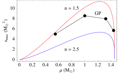
Figure 1: The maximum spin angular momentum $s_{\mathrm{max}}$ vs. mass $\mu$ for a rigidly rotating white dwarf. We plot curves for $n=1.5$ and $n=2.5$ polytropic approximations using Eq. (24), together with four points derived using a more realistic numerical white dwarf model (Geroyannis and Papasotiriou (Geroyannis and Papasotiriou, 2000)).

Note from Eq. (24) that $s_{\mathrm{max}}/\mu^{2}\propto\mu^{-2/3}$ for $\mu\ll\mu_{\mathrm{max}}$, so that the spin per unit mass squared is unbounded as $\mu\rightarrow 0$. Nevertheless, the spin parameter $S_{\mathrm{max}}$ is bounded, since $S_{\mathrm{max}}\propto s_{\mathrm{max}}/\mu\propto\mu^{1/3}$ in the low mass limit. We plot $s_{\mathrm{max}}/\mu$ vs. $\mu$ in Fig. 2, which shows that the maximum value of $s_{\mathrm{max}}/\mu$ is approximately $9\,M_{\odot}$ (corresponding to a $\mu=0.5\,M_{\odot}$ white dwarf). For a central black hole of mass $M=10^{6}\,M_{\odot}$, we then have

$$S\leq S_{\mathrm{max}}=\frac{s_{\mathrm{max}}}{\mu M}=9\times 10^{-6},$$ (25)

which is small compared to unity.

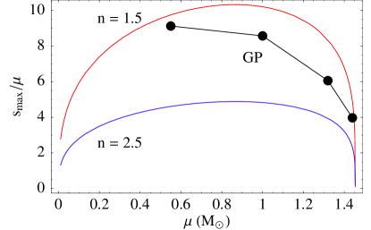
Figure 2: $s_{\mathrm{max}}/\mu$ vs. mass for a white dwarf. As in Fig. 1, we plot curves for $n=1.5$ and $n=2.5$ polytropes and the numerical model from (Geroyannis and Papasotiriou, 2000). The corresponding spin parameter $S_{\mathrm{max}}$ is obtained simply by dividing $s_{\mathrm{max}}/\mu$ by the mass $M$ of the central black hole.

II.2.2 Tidal disruption

We can obtain a higher value of $S$ if the central black hole mass is smaller, but it is important to bear in mind that such lower-mass black holes may tidally disrupt the white dwarf companion, thereby violating a necessary condition for the validity of the Papapetrou equations. In order of magnitude, a white dwarf orbiting at radius $r$ will be disrupted when the tidal acceleration due to the central body overcomes its self-gravity, i.e.,

$$\frac{GM}{r^{3}}R\geq\frac{G\mu}{R^{2}}.$$ (26)

For the white dwarf to be undisrupted down to the horizon at $r=M$, we must have $M\leq R^{3/2}\mu^{-1/2}$, so that [using Eq. (20)] the minimum mass not to disrupt is $M_{\mathrm{min}}\propto\mu^{-1}$. We could evaluate the proportionality constant using Eq. (20), but we can obtain a more accurate result by adopting a constant based on a more realistic tidal disruption model. Tables 1 and 2 of Wiggins and Lai (2000) give the value of the variable $\hat{r}\equiv\displaystyle{\frac{r}{R}\left(\frac{\mu}{M}\right)^{1/3}}$, which is approximately $2.0$ for the white dwarfs of interest here. This gives

$$M_{\mathrm{min}}=2.0^{-3/2}\,R^{3/2}\mu^{-1/2},$$ (27)

as illustrated in Fig. 3. For a $1.0\,M_{\odot}$ white dwarf, which (based on Geroyannis and Papasotiriou (2000)) has $s_{\mathrm{max}}=8.57\,M^{2}_{\odot}$, the central black hole must satisfy $M_{\mathrm{min}}=8.2\times 10^{4}\,M_{\odot}$, so that the spin parameter $S$ can be no bigger than $S_{\mathrm{max}}=s_{\mathrm{max}}/(\mu M_{\mathrm{min}})=1.0\times 10^{-4}$ in order to avoid tidal disruption.

Figure 3: The minimum black hole mass $M$ required not to disrupt an inspiraling corotating white dwarf before the last stable (prograde) circular orbit around a maximally rotating Kerr black hole, as a function of white dwarf mass $\mu$.

II.2.3 The $S=1$ limit

We have shown that all physically realistic cases satisfy $S\ll 1$, but we nevertheless consider the limit of $S=1$ (corresponding to $\mu=M$) in order to investigate more thoroughly the dynamics of the Papapetrou equations, and to compare our results with Suzuki and Maeda (1997), which investigates the $S=1$ limit in detail. The $S=1$ limit introduces no singularities into the equations of motion, and the resulting orbits are valid solutions of the equations. On the other hand, in this limit the Papapetrou equations are not physically realistic, since they are derived in the limit of spinning test particles, which must satisfy $\mu\ll M$. We thus cannot draw reliable results about the behavior of astrophysical systems from the $S=1$ limit.

II.3 Symmetries and the parameterization of initial conditions

In the approximation represented by the Papapetrou equations there is still a constant of the motion associated with each Killing vector $\vec{\xi}$ of the spacetime (Dixon, 1970):

$$C_{\xi}=\xi^{\mu}p_{\mu}-\textstyle{1\over 2}\xi_{\mu;\nu}S^{\mu\nu}.$$ (28)

[For brevity, we write the constant in terms of the spin tensor $S^{\mu\nu}$ [Eq. (12)].] Since Kerr spacetime is stationary and axially symmetric, it has the Killing vectors $\vec{\xi}^{t}=\partial/\partial t$ and $\vec{\xi}^{\phi}=\partial/\partial\phi$, so the energy $E$ and $z$ angular momentum $J_{z}$ are conserved:

$$E=-p_{t}+\textstyle{1\over 2}g_{t\mu,\nu}S^{\mu\nu}$$ (29)

and

$$J_{z}=p_{\phi}-\textstyle{1\over 2}g_{\phi\mu,\nu}S^{\mu\nu}.$$ (30)

(We write $J_{z}$ in place of the orbital angular momentum $L_{z}$ since the spin also contributes to the angular momentum of the system.) In contrast to the energy and momentum integrals, the Carter constant $Q$ is no longer present when the test particle has nonvanishing spin (Tanaka et al., 1996).

In our problem there are twelve variables, four each for position, momentum, and spin. For the purposes of finding orbits by numerical integration, we may parameterize the initial conditions by providing $\tau=0$, $r$, $\theta$, $\phi=0$, $p_{r}$, $E$, $J_{z}$, $S$, and any two of the spin components. The normalization conditions $p_{\mu}p^{\mu}=-1$ and $S_{\mu}S^{\mu}=S^{2}$ allow us to eliminate one component each of momentum and spin. The constraint $p^{\mu}S_{\mu}=0$ and the integrals of the motion then give three equations in three unknowns:

$$0 = p_{\mu}S_{\nu}g^{\mu\nu}$$ (31)

$$E = -p_{t}+\textstyle{1\over 2}g_{t\mu,\nu}S^{\mu\nu}$$ (32)

$$J_{z} = p_{\phi}-\textstyle{1\over 2}g_{\phi\mu,\nu}S^{\mu\nu}$$ (33)

We must solve these equations for the two remaining components of $p_{\mu}$ and one remaining component of $S_{\mu}$. In Schwarzschild spacetime these can be solved explicitly due to the greater symmetry (Suzuki and Maeda, 1997), but in the Kerr case of interest here the problem requires numerical root finding.

We also use a related parameterization method starting with the Kerr geodesic orbital parameters: eccentricity $e$, inclination angle $\iota$, and pericenter $r_{p}$. We derive the corresponding energy, angular momentum, and relevant momenta, and then proceed as above. This method is discussed further in Sec. VII.1.3.

III Lyapunov exponents

III.1 General discussion of Lyapunov exponents

Our method for calculating Lyapunov exponents is well-established in the literature of nonlinear dynamical systems (Alligood et al., 1997; Ott, 1993), but accessible treatments are hard to find in the physics literature, so we summarize the method here. Our discussion is informal and oriented toward practical calculation, based on Ref. (Alligood et al., 1997); for a more formal, rigorous presentation see Eckmann and Ruelle (Eckmann and Ruelle, 1985).

First we give an overview of the methods for calculating Lyapunov exponents most commonly used in physics. Given an initial condition, a set of differential equations determines a solution (the flow), which is a curve in the phase space. The Lyapunov exponents of the flow measure the rate at which nearby trajectories separate. As discussed in the introduction, an orbit is chaotic if a nearby phase-space trajectory separated by an initial distance $\epsilon_{0}$ separates exponentially: $\epsilon(\tau)=\epsilon_{0}\,e^{\lambda\tau}$, where $\lambda$ is the Lyapunov exponent.

Implicit in the definition of chaos above is a notion of a distance function on the phase space (or, more properly, the tangent space to the phase space, as in Eq. (36) below). It is conventional to use a Euclidean metric to define such lengths Alligood et al. (1997); Ott (1993), but any positive-definite nondegenerate metric will do (Eckmann and Ruelle, 1985). While the magnitude of the resulting exponent obviously depends on the particular metric used, the signs of the Lyapunov exponents are a property of the dynamical system and do not rely on any underlying metric structure. We discuss these issues further in Sec. IV.1 and Sec. VII.4.

This informal definition of Lyapunov exponents leads to a practical method for calculating $\lambda$: given an initial condition, consider a nearby initial condition a distance $\epsilon_{0}$ away, where $\epsilon_{0}$ is “small”, typically $10^{-5}$–$10^{-7}$ of the relevant physical scales. (Values of $\epsilon_{0}$ much smaller than this can result in a loss of numerical precision.) Keeping track of the deviation vector between the two points yields a numerical approximation of $\lambda$. (It is important to rescale the deviation vector if it grows too large, since for any bounded phase space flow even a tiny deviation can grow to at most the size of the bounded region.) We call this approach the deviation vector method.

There are two primary limitations to the approach outlined above. First, the method yields only the largest Lyapunov exponent, which is sufficient to establish the presence of chaos but paints a limited picture of the dynamics. Second, the deviation vector approach is most appropriate when an analytical expression for the Jacobian matrix is unknown; by choosing $\epsilon_{0}$ small enough (and by keeping $\epsilon(\tau)$ small by rescaling if necessary), the method essentially takes a numerical derivative. Among other complications, the value of the exponent depends both on the maximum allowable size $\epsilon_{\mathrm{max}}$ (the size at which the deviation is rescaled) and the initial value $\epsilon_{0}$ (the size of the deviation after each rescaling).

The principal virtue of the deviation vector approach compared to the more complicated Jacobian method (discussed below) is speed, since it requires solving only the equations of motion. (As we discuss in Sec. III.2.1, the Jacobian method involves the time-consuming evolution of the Jacobian matrix in parallel with the equations of motion.) It also provides a valuable way to verify the validity of the Jacobian method.

The Jacobian method is a more thorough and rigorous approach to the calculation of Lyapunov exponents, which makes precise the notion of “infinitesimally” separated vectors. The general method proceeds as follows: consider a phase space with variables ${\bf y}=\{y_{i}\}$ and an autonomous set of differential equations

$$\frac{d\mathbf{y}}{d\tau}=\mathbf{f}(\mathbf{y}).$$ (34)

(Here we use $\tau$ instead of $t$ in anticipation of the application of these results to general relativity, where we will be using proper time as our time parameter.) If $\delta{\bf y}$ represents a small deviation vector, then the distance between the two trajectories is

$$\frac{d(\delta{\bf y})}{d\tau}={\bf f}({\bf y}+\delta{\bf y})-{\bf f}({\bf y})={\bf Df}\cdot\delta{\bf y}+{\cal O}(\|\delta{\bf y}\|^{2}),$$ (35)

where ${\bf Df}$ is the Jacobian matrix [$({\bf Df})_{ij}=\partial f_{i}/\partial x^{j}$].

We can clarify the notation and make the system easier to visualize if we introduce $\bm{\xi}$ as an element of the tangent space at ${\bf y}$, so that

$$\frac{d\bm{\xi}}{d\tau}={\bf Df}\cdot\bm{\xi},$$ (36)

which is equivalent to taking the limit $\|\delta{\bf y}\|\rightarrow 0$. We visualize $\bm{\xi}$ as a perfectly finite vector (as opposed to an “infinitesimal”). Since it lives in the tangent space, not the physical phase space, $\bm{\xi}$ can grow arbitrarily large with time. This means that instead of the frequent rescaling required in the deviation vector approach, $\bm{\xi}$ must be rescaled only when it grows so large that it approaches the floating point limit of the computer. This is a rare occurrence, and in practice the tangent vector almost never needs rescaling.

Although following the evolution of an arbitrary initial tangent vector $\bm{\xi}$ yields the largest Lyapunov exponent, we can do even better by following the evolution of a family of $n$ tangent vectors, which allows us to determine all $n$ Lyapunov exponents. The essence of the method is as follows: for a system of differential equations with $n$ variables, we consider a set of $n$ vectors that lie on a ball in the tangent space. We represent this ball using a matrix whose columns are $n$ normalized, linearly independent tangent vectors, conventionally taken to be orthogonal. This set of orthonormal vectors then spans a unit ball in the tangent space. The action of the Jacobian matrix, which is a linear operator on the tangent space, is to map the ball to an ellipsoid under the time-evolution of the flow, as shown in Fig. 4.

Figure 4: The Jacobian matrix maps a tangent space ball to an ellipsoid.

For a dynamical system with $n$ degrees of freedom, there are $n$ Lyapunov numbers that measure the average growth of the $n$ principal axes $\{r_{i}(\tau)\}_{i=1}^{n}$ of the ellipsoid. More formally, the Lyapunov numbers $L_{i}$ are given by

$$L_{i}=\lim_{\tau\rightarrow\infty}[r_{i}(\tau)]^{1/\tau},$$ (37)

where $r_{i}(\tau)$ is the length of the $i$th principal axis of the ellipsoid. The corresponding Lyapunov exponents are the natural logarithms of the Lyapunov numbers, so that

$$\lambda_{i}=\lim_{\tau\rightarrow\infty}\frac{\log\,[r_{i}(\tau)]}{\tau}.$$ (38)

These limits exist for a broad class of dynamical systems (Eckmann and Ruelle, 1985).

The principal axes of the tangent space ellipsoid indicate the directions along which nearby initial conditions separate or converge, which we may call the Lyapunov directions. In particular, consider a principal axis that is stretched under the time evolution. Such a vector has one component for each dimension (position or momentum) in the phase space; a nonzero component in any direction indicates an exponential divergence in the corresponding coordinate. For example, if a system has two spatial coordinates $(r,\phi)$ and corresponding momenta $(p_{r},p_{\phi})$, then a typical tangent vector will have components $\bm{\xi}=(\xi_{r},\xi_{\phi},\xi_{p_{r}},\xi_{p_{\phi}})$. If the only tangent vector with nonzero Lyapunov exponent is, for example, $\bm{\xi}={1\over\sqrt{3}}(1,1,1,0)$, then nearby initial conditions separate exponentially in $r$, $\phi$, and $p_{r}$, but nearby values of $p_{\phi}$ do not separate exponentially. This is potentially relevant to the present study since, in the limit of a point test particle, the gravitational radiation depends on the spatial variables but not the spin. If the principal axes along expanding directions have nonzero components only in the spin directions, the system could be formally chaotic without affecting the gravitational waves.

In summary, the method for visualizing the Lyapunov exponents of a dynamical system is to picture a ball of initial conditions—an infinitesimal ball if visualized in the phase space, or a unit ball if visualized in the tangent space—and watch it evolve into an ellipsoid under the action of the Jacobian matrix. After a sufficiently long time, the ellipsoid will be greatly deformed, stretched out along the expanding directions and compressed along the contracting directions. The directions of the principal axes are the Lyapunov directions, and their lengths give the Lyapunov numbers through the relation $L_{i}\approx[r_{i}(\tau)]^{1/\tau}$.

III.2 Numerical calculation of Lyapunov exponents

In order to implement a numerical algorithm based on the considerations above, we must bear two things in mind. First, since the vectors spanning the initial unit ball are arbitrary, they will all be stretched in the direction of the largest exponent: in general every initial vector has some nonzero component along the direction of greatest stretching, which dominates as $\tau\rightarrow\infty$. In order to find the other principal axes, we must periodically produce a new orthogonal basis. We will show that the Gram-Schmidt procedure is appropriate. Second, the lengths of the vectors could potentially overflow or underflow the machine precision, so we should periodically normalize the ellipsoid axes.

III.2.1 The algorithm in detail

To simplify the notation, we denote the (time-dependent) Jacobian matrix $\mathbf{Df}$ by $J_{\tau}$ and the ellipsoid (whose columns are the tangent vectors) by $U$. The algorithm then proceeds as follows:

1. Construct a set of $n$ orthonormal vectors (which span an $n$-dimensional ball in the tangent space of the flow). Represent this ball by a matrix $U$ whose columns are the tangent vectors $\bm{\xi}_{i}$.

2. Eq. (36), applied to each tangent vector, implies that $U$ satisfies the matrix equation

   $$\frac{dU}{d\tau}=J_{\tau}\,U,$$ (39)

   which constitutes a set of linear differential equations for the tangent vectors. Since $J_{\tau}$ depends on the values of $\mathbf{y}$, these equations are coupled to our system of nonlinear differential equations $\dot{\mathbf{y}}=\mathbf{f}(\mathbf{y})$, so they must be solved in parallel with Eq. (34).

3. Choose some time $T$ big enough to allow the expanding directions to grow but small enough so that they are not too big. Numerically integrate Eqs. (34) and (39), and every time $T$ apply the Gram-Schmidt orthogonalization procedure. The vectors resulting from the Gram-Schmidt procedure approximate the semiaxes of the evolving ellipsoid. Record the log of the length $\log\,[r_{i}(\tau_{n})]$ of each vector after each time $T$, where $\tau_{n}=nT$. Finally, normalize the ellipsoid back to a unit ball.

4. At each time $\tau$, the sum

   $$\lambda_{i}\approx{1\over\tau}\sum_{n=1}^{N}\log\,[r_{i}(\tau_{n})]\equiv\frac{\log\,[r_{i}(\tau)]}{\tau}$$ (40)

   is a numerical estimate for the $i$th Lyapunov exponent.

III.2.2 Gram-Schmidt and Lyapunov exponents

The use of the Gram-Schmidt procedure is crucial to extracting all $n$ Lyapunov exponents. Let us briefly review this important construction. Given $n$ linearly-independent vectors $\{{\bf u}_{i}\}$, the Gram-Schmidt procedure constructs $n$ orthogonal vectors $\{{\bf v}_{i}\}$ that span the same space, given by

$${\bf v}_{i}={\bf u}_{i}-\sum_{j=1}^{i-1}\frac{{\bf u}_{i}\cdot{\bf v}_{j}}{\|{\bf v}_{j}\|^{2}}\,{\bf v}_{j}.$$ (41)

To construct the $i$th orthogonal vector, we take the $i$th vector from the original set and subtract off its projections onto the previous $i-1$ vectors produced by the procedure.

The use of Gram-Schmidt in dynamics comes from observing that the resulting vectors approximate the semiaxes of the tangent space ellipsoid. After the first time $T$, all of the vectors point mostly along the principal expanding direction. We may therefore pick any one as the first vector in the Gram-Schmidt algorithm, so choose $\bm{\xi}_{1}\equiv{\bf u}_{1}$ without loss of generality. If we let ${\bf e}_{i}$ denote unit vectors along the principal axes and let $r_{i}$ be the lengths of those axes, the dynamics of the system guarantees that the first vector ${\bf u}_{1}$ satisfies

$${\bf u}_{1}=r_{1}{\bf e}_{1}+r_{2}{\bf e}_{2}+\cdots\approx r_{1}{\bf e}_{1}\equiv{\bf v}_{1}$$

since ${\bf e}_{1}$ is the direction of fastest stretching. The second vector ${\bf v}_{2}$ given by Gram-Schmidt is then

$${\bf v}_{2}={\bf u}_{1}-\frac{{\bf u}_{1}\cdot{\bf v}_{1}}{\|{\bf v}_{1}\|^{2}}\,{\bf v}_{1}\approx{\bf u}_{1}-r_{1}{\bf e}_{1}=r_{2}{\bf e}_{2},$$

with an error of order $r_{2}/r_{1}$. The procedure proceeds iteratively, with each successive Gram-Schmidt step (approximately) subtracting off the contribution due to the previous semiaxis direction.

It is important to choose time $T$ long enough to keep errors of the form $r_{2}/r_{1}$ small but short enough to prevent numerical under- or overflow. In practice, the method is quite robust, and it is easy to find valid choices for the time $T$, as discussed in Sec. VII.

IV Relativity and Papapetrou subtleties

The algorithm described above is of a general nature, designed with a generic dynamical system in mind. The Papapetrou equations and the framework of general relativity present additional complications. Here we discuss some refinements to the algorithm necessary for the present case.

IV.1 Phase space norm

In the context of general relativistic dynamical systems, the meaning of trajectory separation in phase space is somewhat obscured by the time variable. We can skirt the issue of trajectories “diverging in time” by using a $3+1$ splitting of spacetime, and consider trajectory separation in a spacelike hypersurface (Karas and Vokrouhlický, 1992). This prescription reduces properly to the traditional method for classical dynamical systems in the nonrelativistic limit.

In Kerr spacetime, we use the zero angular-momentum observers (ZAMOs), and project 4-dimensional quantities into the ZAMO hypersurface using the projection tensor $P^{\mu}_{\ \nu}=\delta^{\mu}_{\ \nu}+U^{\mu}U_{\nu}$, where $U^{\mu}$ is the ZAMO 4-velocity. In this formulation, spatial variables obey $x^{\mu}\rightarrow\tilde{x}^{i}=P^{i}_{\ \mu}\,x^{\mu}$ and momenta obey $p_{\mu}\rightarrow\tilde{p}_{i}=P^{\mu}_{\ i}\,p_{\mu}$ (and similarly for $S_{\mu}$) (Karas and Vokrouhlický, 1992). The relevant norm is then a Euclidean distance in the 3-dimensional hypersurface.

We should note that we use the projected norm for conceptual clarity, not necessity. The naive use of a Euclidean norm using unprojected components yields the same sign for the exponents, as noted in Sec. III.1. The magnitudes of the resulting exponents are also similar (Sec. VII.4).

IV.2 Constraint complications

Although the Lyapunov algorithm is fairly straightforward to implement for a general dynamical system, the constrained nature of the Papapetrou equations adds a considerable amount of complexity. The fundamental problem is that the tangent vector $\bm{\xi}$ cannot have arbitrary initial components for the Papapetrou system, as it can for an unconstrained dynamical system. Each $\bm{\xi}$ must correspond to some deviation $\delta\mathbf{y}$ which is not arbitrary: the deviated point $\mathbf{y}+\delta\mathbf{y}$ must satisfy the constraints.

IV.2.1 Constraint-satisfying deviations

Recall that the dynamical variables in the Papapetrou equations must satisfy normalization and orthogonality constraints (Sec. II.1): $p^{\nu}p_{\nu}=-1$ (normalized units), $S^{\nu}S_{\nu}=S^{2}$, and $p^{\nu}S_{\nu}=0$. To make the constraint condition on $\delta{\bf y}$ clearer, let $\mathbf{C}\mathbf{(}\mathbf{y})=0$ represent the constraints rearranged so that the right hand side is zero. For example, with ${\mathbf{y}}=(t,r,\mu,\phi,p_{t},p_{r},p_{\mu},p_{\phi},S_{t},S_{r},S_{\mu},S_{\phi})$, we can write

$$C_{1}({\mathbf{y}})=p^{\nu}p_{\nu}+1,$$ (42)

so that $C_{1}({\mathbf{y}})=0$ for a constraint-satisfying ${\mathbf{y}}$. The other constraints are then

$$C_{2}({\mathbf{y}})=S^{\nu}S_{\nu}-S^{2}$$ (43)

and

$$C_{3}({\mathbf{y}})=p^{\nu}S_{\nu}.$$ (44)

A deviation $\delta\mathbf{y}$ is constraint-satisfying if ${\mathbf{C}}({\mathbf{y}}+\delta{\mathbf{y}})={\bf 0}$ when ${\mathbf{C}}({\mathbf{y}})={\bf 0}$.

We may construct a constraint-satisfying deviation $\delta{\mathbf{y}}$ as follows. Begin with a 12-dimensional vector ${\bf y}$ that satisfies the constraints. Add a random small deviation to eight of its components to form a new vector ${\bf y}^{\prime}$. (We need not add a deviation to $t$; see Sec. IV.2.2 below.) Determine the remaining three components of ${\bf y}^{\prime}$ using the constraints, using the same technique used to set the initial conditions. Finally, set $\delta{\bf y}\equiv{\bf y}^{\prime}-{\bf y}$. The corresponding $\bm{\xi}$ is then simply $\delta{\mathbf{y}}/\|\delta{\mathbf{y}}\|$.

The prescription above glosses over an important detail: the inference of tangent vector components from the constraints is not unique. Solving the constraint equations involves taking square roots in several places, so there are a number of sign ambiguities representing different solution branches. The implementation of the component-inference algorithm must compare each component of ${\bf y}$ with the corresponding component of ${\bf y}^{\prime}$ to ensure that they represent solutions from the same branches. Enforcing the constraints in this manner, and thereby inferring the full tangent vector $\bm{\xi}$, is especially important for the algorithm described in the next section.

IV.2.2 A modified Gram-Schmidt algorithm

A spinning test particle has an apparent twelve degrees of freedom—four each for position, momentum, and spin—so a priori there is the potential for twelve nonzero exponents. Since the Papapetrou equations have no explicit time-dependence, we can eliminate the time degree of freedom. The three constraints (momentum and spin normalization, and momentum-spin orthogonality) further reduce the number of degrees of freedom by three. We are left finally with eight degrees of freedom.

Eliminating the four spurious degrees of freedom from the tangent vectors presents a formidable obstacle to the implementation of the phase space ellipsoid method described in Sec. III.2.1. The crux of the dilemma is that the axes of the ellipsoid must be orthogonal, but must also correspond to constraint-satisfying deviation vectors—mutually exclusive conditions. Solving this problem requires a modification of the Gram-Schmidt algorithm:

1. Instead of a $12\times 12$ ball (i.e., $n=12$ in the original algorithm), consider an $8\times 8$ ball by choosing to eliminate the $t$, $p_{t}$, $p_{\phi}$, and $S_{t}$ components. The time component $\xi_{t}$ of each tangent vector is irrelevant since nothing in the problem is explicitly time dependent; the first column of the Jacobian matrix is zero, so $\xi_{t}$ is not necessary to determine the time-evolution. The other three components are determined by the constraints as described above.

2. Given eight initial random tangent vectors, apply the Gram-Schmidt process to form an $8\times 8$ ball. For each vector, determine the three missing components using the constraints, and then evolve the system using

   $$\frac{dU}{d\tau}=J_{\tau}U$$

   as before. (Now $U$ represents a $12\times 8$ matrix instead of a $12\times 12$ ball.)

3. At each time $T$, extract the relevant eight components from each vector to form a new $8\times 8$ ellipsoid, apply Gram-Schmidt, and then fill in the missing components using the constraints, yielding again a $12\times 8$ matrix. The projected norms of the eight tangent vectors contribute to the running sums for the Lyapunov exponents as in the original algorithm.

The algorithm above yields eight Lyapunov exponents for the Papapetrou system of equations.

In order to implement this algorithm, we must have a method for constructing a full tangent vector $\bm{\xi}$ from an eight-component vector $\tilde{\bm{\xi}}$. The method is as follows:

1. Let $\tilde{\bf y}^{\prime}={\bf y}+\epsilon\tilde{\bm{\xi}}$ for a suitable choice of $\epsilon$.

2. Fill in the missing components of $\tilde{\bf y}^{\prime}$ using the constraints to form ${\bf y}^{\prime}$, taking care that ${\bf y}$ and ${\bf y}^{\prime}$ have the same constraint branches.

3. Infer the full tangent vector using $\bm{\xi}=\displaystyle{\frac{{\bf y}^{\prime}-{\bf y}}{\epsilon}}$.

This technique depends on the choice of $\epsilon$, and fails when $\epsilon$ is too small or too large. Using the techniques discussed in the next section to calibrate the system, we find that $\epsilon\approx 10^{-5}$–$10^{-6}$ works well in practice.

IV.2.3 Two rigorous techniques

It should be clear from the discussion above that extracting all eight Lyapunov exponents is difficult, and in practice the techniques are finicky, depending (among other things) on the choice of $\epsilon$ as described in Sec. IV.2.2 above. How, then, can we be confident that the results make sense? Fortunately, there are two techniques that give rigorous Lyapunov exponents by managing to sidestep the constraint complexities entirely.

First, it is always possible to calculate the single largest exponent using the Jacobian method without considering the constraint subtleties. The complexity of the main Jacobian approach involves the competing requirements of Gram-Schmidt orthogonality and constraint satisfaction, but in the case of only one vector these difficulties vanish. Since the equations of motion preserve the constraints, an initial constraint-satisfying tangent vector retains this property throughout the integration. Thus, we begin with a vector constructed as in Sec. IV.2.1 and evolve it (without rescaling) along with the equations of motion. Other than the requirement of constraint satisfaction, its initial components are arbitrary, so it evolves in the direction of largest stretching and eventually points in the largest Lyapunov direction. The logarithm of its projected norm then contributes to the sum for the largest Lyapunov exponent.

Second, we can implement a deviation vector approach as described in Sec. III.1. Given an initial condition ${\bf y}_{0}$, we construct a nearby initial condition ${\bf y}^{\prime}_{0}$ as in Sec. IV.2.1 and then evolve them both forward. In principle, an approximation for the largest Lyapunov exponent is then $\displaystyle{{1\over\tau}\log\left(\frac{\|{\bf y}^{\prime}-{\bf y}\|}{\|{\bf y}^{\prime}_{0}-{\bf y}_{0}\|}\right)\equiv{1\over\tau}\log\left(\frac{\|\delta{\bf y}\|}{\|\delta{\bf y}_{0}\|}\right)}$. In practice (for chaotic systems) the method saturates: for a given initial deviation, say $\|\delta{\bf y}_{0}\|\sim 10^{-6}$, once the initial conditions have diverged by a factor of $\sim\!\!10^{6}$ the method breaks down. (The traditional solution to the saturation problem is to rescale the deviation before it saturates, but such a rescaling in this case violates the constraints.) Despite its limitations, this unrescaled deviation vector technique is valuable, since it tracks the correct solution until the saturation limit is reached, and avoids the subtleties associated with the constraints.

With these two techniques in hand, we have a powerful method for verifying that the largest Lyapunov exponent produced by the Gram-Schmidt method is correct. This, in turn, gives us confidence that the other Lyapunov exponents produced by the main algorithm are meaningful as well.

V Implementation details

V.1 Some numerical comments

Finally, we discuss some specialized issues related to integrating the Papapetrou equations on a computer. The primary subjects are the formulation of the equations, optimization techniques, and error checking.

Our choice to write the Papapetrou equations using the spin vector is motivated partially by numerical considerations. The spin vector approach has nice properties compared to the tensor approach as $S\rightarrow 0$. Comparing their covariant derivatives is instructive:

$$\nabla_{\vec{v}}\,S_{\mu} = -p_{\mu}\left(R^{*\alpha\ \gamma\delta}_{\ \ \beta}S_{\alpha}v^{\beta}p_{\gamma}S_{\delta}\right)$$

$$\nabla_{\vec{v}}\,S^{\mu\nu} = p^{\mu}v^{\nu}-p^{\nu}v^{\mu}=2p^{[\mu}v^{\nu]}.$$

Though simpler in form, the derivative of $S^{\mu\nu}$ has unfortunate numerical properties for small $S$, since in the limit $S\rightarrow 0$ we have $p^{\mu}\rightarrow v^{\mu}$: the difference $p^{\mu}v^{\nu}-p^{\nu}v^{\mu}$ goes to zero in principle but in practice is plagued by numerical roundoff errors. Since $S\ll 1$ is the most physically interesting limit, the vector approach is more convenient for our purposes.

Calculating the many tensors and derivatives which go into the Papapetrou equations and the corresponding Jacobian matrix is a considerable task. As a first step, we use GRTensor for Maple to calculate all relevant quantities, and we use Maple’s optimized C output to create C code automatically. Due to the symmetries of the Riemann tensor and the metric, many terms are identically zero, which significantly reduces the number of required operations. For example, in order to calculate $R^{*\alpha\ \gamma\delta}_{\ \ \beta}S_{\alpha}v^{\beta}p_{\gamma}S_{\delta}$ we need four loops, which constitutes $4^{4}=256$ evaluations, but in fact $R^{*\alpha\ \gamma\delta}_{\ \ \beta}$ has only 80 nonzero components. Performing loop unrolling by writing these terms to an optimized derivatives file consisting of explicit sums speeds up calculation by an order of magnitude compared to nested for loops.

Another optimization involves the choice of coordinates used in the metric, which has significant consequences for the size of the tensor files and the number of floating point operations required. Simply using $\mu=\cos\theta$ in the Kerr metric reduces the size of the Riemann derivatives by at least a factor of two. Since these derivatives are the bottleneck in the calculation of the Jacobian matrix, we can get more than a 50% improvement in performance with even this simple variable transformation.

All integrations were performed using a Bulirsch-Stoer integrator adapted from Numerical Recipes (Press et al., 1992). Occasional checks with a fifth-order Runge-Kutta integrator were in agreement. We verified the Papapetrou integration by checking errors in the constraints and conserved quantities; for an orbit such as that shown in Fig. 6, all errors are at the $10^{-11}$ level after $\tau=10^{5}\,M$.

As should be clear from Sec. V.2 below, the Jacobian matrix of the Papapetrou equations has a large number of terms, and it is essential to verify its correctness by using a diagnostic that compares $\mathbf{Df}\cdot\delta\mathbf{y}$ with the difference $\mathbf{f}(\mathbf{y}+\delta\mathbf{y})-\mathbf{f}(\mathbf{y})$ for a suitable constraint-satisfying $\delta\mathbf{y}$. It is not sufficient for the difference merely to be small: we must calculate the quantity $\mathbf{f}(\mathbf{y}+\delta\mathbf{y})-\mathbf{f}(\mathbf{y})-{\bf Df}\cdot\delta{\bf y}$ for several values of $\delta{\bf y}$ and verify that each component scales as $\|\delta{\bf y}\|^{2}$. An early implementation of the Jacobian matrix, which gave nearly identical results for $\mathbf{f}(\mathbf{y}+\delta\mathbf{y})-\mathbf{f}(\mathbf{y})$ and ${\bf Df}\cdot\delta{\bf y}$, nevertheless had an undetected ${\cal O}(S^{2})$ error. The unrescaled deviation vector approach showed a discrepancy with the Jacobian method, which showed spurious chaotic behavior. The $\|\delta{\bf y}\|^{2}$ scaling method described above eventually diagnosed the problem, which resulted from a missing term in $\partial\dot{S}_{\mu}/\partial S_{\nu}$ (Sec V.2).

V.2 The Jacobian matrix

For reference, we write out explicit equations for part of the Jacobian matrix of the Papapetrou equations.

The Jacobian matrix of a system of differential equations, specialized to the case at hand, is as follows:

$$\left(\begin{array}[]{rcl}\displaystyle{\frac{\partial\dot{x}^{\mu}}{\partial x^{\nu}}}&\displaystyle{\frac{\partial\dot{x}^{\mu}}{\partial p_{\nu}}}&\displaystyle{\frac{\partial\dot{x}^{\mu}}{\partial S_{\nu}}}\vskip 6.0pt plus 2.0pt minus 2.0pt\\ \displaystyle{\frac{\partial\dot{p}_{\mu}}{\partial x^{\nu}}}&\displaystyle{\frac{\partial\dot{p}_{\mu}}{\partial p_{\nu}}}&\displaystyle{\frac{\partial\dot{p}_{\mu}}{\partial S_{\nu}}}\vskip 6.0pt plus 2.0pt minus 2.0pt\\ \displaystyle{\frac{\partial\dot{S}_{\mu}}{\partial x^{\nu}}}&\displaystyle{\frac{\partial\dot{S}_{\mu}}{\partial p_{\nu}}}&\displaystyle{\frac{\partial\dot{S}_{\mu}}{\partial S_{\nu}}}\\ \end{array}\right)$$ (45)

Once we calculate $\partial\dot{x}^{\mu}/\partial x^{\nu}=v^{\mu}_{\ ,\nu}$, all the other derivatives can be expressed in terms of the derivatives of $v^{\mu}$, the tensors and connection coefficients, and Kronecker $\delta$s.

Written out in full, and the Papapetrou equations are as follows:

$$\dot{x}^{\mu} = v^{\mu}$$ (46)

$$\dot{p}_{\mu} = -R^{*\ \ \alpha\beta}_{\mu\nu}v^{\nu}p_{\alpha}S_{\beta}+\Gamma^{\alpha}_{\ \beta\mu}p_{\alpha}v^{\beta}$$ (47)

$$\dot{S}_{\mu} = -p_{\mu}\left(R^{*\alpha\ \gamma\delta}_{\ \ \beta}S_{\alpha}v^{\beta}p_{\gamma}S_{\delta}\right)+\Gamma^{\alpha}_{\ \beta\mu}S_{\alpha}v^{\beta}$$ (48)

We measure $\tau$ and $r$ in units of $M$ (the mass of the central body), $p_{\mu}$ in units of the particle rest mass $\mu$, and $S_{\mu}$ in terms of the product $\mu M$. The overdot is an ordinary derivative with respect to proper time: $\dot{x}\equiv dx/d\tau$.

The unusual placement of indices on $R^{*}$ is motivated by the form of the Jacobian matrix. The index placement shown above brings the equations into a form where the indices on $p_{\mu}$ and $S_{\mu}$ are always lowered, which simplifies the Jacobian matrix since (for example) $\partial p_{\mu}/\partial x^{\mu}=0$. Otherwise the Jacobian matrix is unnecessarily complicated; for example, if $p^{\mu}$ appeared anywhere on the right hand side then we would have $\partial p^{\mu}/\partial x^{\nu}\neq 0$, which would contribute to $J_{\tau}$.

As discussed in Sec II.1, the supplementary condition $p_{\mu}S^{\mu\nu}=0$ [Eq. (6)] leads to the equation for $v^{\mu}$ in terms of $p^{\mu}$:

$$v^{\mu}=N(p^{\mu}+w^{\mu})=N\tilde{v}^{\mu},$$ (49)

where

$$\tilde{v}^{\mu}=p^{\mu}+w^{\mu}$$ (50)

and

$$w^{\mu}=-{{}^{*}}R^{*\mu\alpha\beta\gamma}S_{\alpha}p_{\beta}S_{\gamma}.$$ (51)

$N$ is a normalization constant fixed by $v_{\mu}v^{\mu}=-1$.

The calculation of the partial derivatives $\dot{x}^{\mu}$ in Eq. (45) proceeds as follows. From the relation for $v^{\mu}=N\tilde{v}^{\mu}$, we have

$$\frac{\partial\dot{x}^{\mu}}{\partial x^{\nu}}=v^{\mu}_{\ ,\nu}=N\tilde{v}^{\mu}_{\ ,\nu}+N_{,\nu}\tilde{v}^{\mu}.$$

Now, $\tilde{v}^{\mu}_{\ ,\nu}=p^{\mu}_{\ ,\nu}+w^{\mu}_{\ ,\nu}=p_{\alpha}g^{\alpha\mu}_{\ \ ,\nu}-{{}^{*}}R^{*\mu\alpha\beta\gamma}_{\ \ \ \ \ \ ,\nu}S_{\alpha}p_{\beta}S_{\gamma}$, so the first term is easy. The second term is trickier: from the expression for $v^{\mu}$, we have that $-1=v^{\mu}v_{\mu}=N^{2}(p^{\mu}p_{\mu}+2w^{\mu}p_{\mu}+w^{\mu}w_{\mu})=N^{2}(-1+2w^{\mu}p_{\mu}+w^{\mu}w_{\mu})$, so we have

$$N=(1-2w^{\mu}p_{\mu}-w^{\mu}w_{\mu})^{-1/2}.$$

Differentiating gives

$$\begin{array}[]{rcl}N_{,\nu}&=&N^{3}\left(p_{\alpha}w^{\alpha}_{\ ,\nu}+w^{\alpha}_{\ ,\nu}w_{\alpha}+\textstyle{1\over 2}w^{\alpha}w^{\beta}g_{\alpha\beta,\nu}\right)\\ &=&N^{3}\left(\tilde{v}_{\alpha}w^{\alpha}_{\ ,\nu}+\textstyle{1\over 2}w^{\alpha}w^{\beta}g_{\alpha\beta,\nu}\right)\end{array}$$

where we have re-labeled the dummy index ($\mu\rightarrow\alpha$). Summing the various terms, we have

$$v^{\mu}_{\ ,\nu} = N\left[p_{\alpha}g^{\alpha\mu}_{\ \ ,\nu}+w^{\mu}_{\ ,\nu}\right.$$ (52)

$$\left.+\,v^{\mu}(v_{\alpha}w^{\alpha}_{\ ,\nu}+\textstyle{1\over 2}Nw^{\alpha}w^{\beta}g_{\alpha\beta,\nu})\right].$$

The expression for $\partial\dot{x}^{\mu}/\partial p_{\nu}$ is similar to $v^{\mu}_{\ ,\nu}$, but it is simpler because the derivative of the metric with respect to the momentum is zero. As before, we use the product rule:

$$\frac{\partial v^{\mu}}{\partial p_{\nu}}=N\frac{\partial\tilde{v}^{\mu}}{\partial p_{\nu}}+\frac{\partial N}{\partial p_{\nu}}\tilde{v}^{\mu}.$$

The first term requires

$$\frac{\partial\tilde{v}^{\mu}}{\partial p_{\nu}}=\frac{\partial p^{\mu}}{\partial p_{\nu}}+\frac{\partial w^{\mu}}{\partial p_{\nu}}=g^{\mu\nu}-{{}^{*}}R^{*\mu\alpha\nu\beta}_{\ \ \ \ \ }S_{\alpha}S_{\beta}\equiv g^{\mu\nu}+W^{\mu\nu}.$$

Note that $W^{\mu\nu}$ is symmetric. The second term requires

$$\frac{\partial N}{\partial p_{\nu}}=N^{3}(W^{\alpha\nu}p_{\alpha}+w^{\alpha}\delta_{\alpha}^{\ \nu}+W^{\alpha\nu}w_{\alpha})=N^{3}(w^{\nu}+\tilde{v}_{\alpha}W^{\alpha\nu}).$$

Summing the terms gives

$$\frac{\partial\dot{x}^{\mu}}{\partial p_{\nu}}=N(g^{\mu\nu}+W^{\mu\nu}+Nv^{\mu}w^{\nu})+Nv^{\mu}v_{\alpha}W^{\alpha\nu}$$ (53)

with

$$\frac{\partial w^{\mu}}{\partial p_{\nu}}\equiv W^{\mu\nu}=-{{}^{*}}R^{*\mu\alpha\nu\beta}_{\ \ \ \ \ }S_{\alpha}S_{\beta}.$$ (54)

Finally, we calculate $\partial\dot{x}^{\mu}/\partial S_{\nu}$. With

$$\frac{\partial\tilde{v}^{\mu}}{\partial S_{\nu}}=-S_{\alpha}p_{\beta}({{}^{*}}R^{*\mu\alpha\beta\nu}-{{}^{*}}R^{*\mu\nu\alpha\beta})\equiv V^{\mu\nu},$$

and

$$\frac{\partial N}{\partial S_{\nu}}\tilde{v}^{\mu}=Nv^{\mu}v_{\alpha}V^{\alpha\nu},$$

we have

$$\frac{\partial\dot{x}^{\mu}}{\partial S_{\nu}}=NV^{\mu\nu}+Nv^{\mu}v_{\alpha}V^{\alpha\nu}.$$ (55)

We calculate the derivatives of $\dot{p}_{\mu}$ and $\dot{S}_{\mu}$ using $v^{\mu}_{\ ,\nu}$, the product rule, and the derivatives of the various tensors in the problem. The full results appear in the appendix.

VI Integrability and chaos

VI.1 Phase space and constants of the motion

Having laid the foundation for the numerical calculation of Lyapunov exponents, we now discuss some general aspects of dynamical systems relevant to our study. A dynamical system with $n$ coordinates has a $2n$ dimensional phase space, typically consisting of generalized positions and their corresponding conjugate momenta. Motion in the phase space is arbitrary in general, but when there are integrals of the motion then the flow is confined to a surface on which the integral is constant. This can be seen most easily by transforming to angle-action coordinates, where the surface is an invariant (multidimensional) torus.

A system with $n$ coordinates and $n$ constants of the motion is integrable and cannot have chaos (though the motion can still be quasiperiodic or exhibit other complicated behavior). For example, we can consider geodesic orbits around a Kerr black hole to have eight degrees of freedom ($n=4$) and four constants of the motion—particle rest mass $\mu$, energy $E$, axial or $z$ angular momentum $L_{z}$, and Carter constant $Q$—which are enough to integrate the equations of motion explicitly. Alternatively, we may look at Kerr spacetime as having a 6-dimensional phase space by eliminating time (which is simply a re-parameterization of the proper time) and using rest mass conservation to eliminate one momentum coordinate. Then the three integrals $E$, $L_{z}$, and $Q$ are sufficient to integrate the motion. (In practice, we allow all four momenta to evolve freely; the normalization is then a constraint which can be checked for consistency at the end of the integration.)

In the case of a spinning test particle, the extra spin degrees of freedom create the possibility for chaotic behavior. Moreover, since $Q$ is not conserved in the case of nonzero spin, even without the extra spin degrees of freedom the potential for chaos would exist. Kerr spacetime has just enough constants to make the system integrable; losing $Q$ reduces the number of analytic integrals below the critical level required to guarantee integrability.

VI.2 Hamiltonian systems

VI.2.1 Lyapunov exponents for Hamiltonian flows

The phase space flow of Hamiltonian systems is constrained by more than the integrals of the motion. In particular, the Lyapunov exponents of a Hamiltonian system come in pairs $\pm\lambda$; i.e., if $\lambda$ is a Lyapunov exponent then so is $-\lambda$ (Eckmann and Ruelle, 1985). Geometrically, this means that if one semimajor axis of the phase-space ellipsoid stretches an amount $e^{\lambda\tau}=L$, another axis must shrink by an amount $e^{-\lambda\tau}=1/L$. One consequence of this property is that the product of the lengths of the axes is 1. Since the ellipsoid volume is proportional to this invariant product, Liouville’s theorem on the conservation of phase space volume follows as a corollary.

The $\pm\lambda$ property of Hamiltonian flows results from the symplectic nature of the Jacobian matrix for Hamiltonian dynamical systems. But a naive analysis of the Jacobian matrix of the Papapetrou equations shows that it is not symplectic in the canonical sense. Nevertheless, the Papapetrou equations can be derived from a Lagrangian (Hojman, 1975), and can be cast in Hamiltonian form by use of a free Hamiltonian with added constraints (following the method of Dirac (Dirac, 1964) as discussed in (Hanson and Regge, 1974)). As a consequence, we could in principle find coordinates in which the Jacobian matrix is symplectic with respect to the canonical symplectic matrix. Fortunately, this is an unnecessary complication, since the underlying dynamics are independent of the coordinates.

VI.2.2 Exponents for spinning test particles

As discussed in Sec. IV.2.2, the lack of explicit time dependence independence and the three constraints reduce the degrees of freedom from twelve to eight, which leaves the possibility of eight nonzero Lyapunov exponents. The phase space flow is further constrained by the constants of the motion, energy and $z$ angular momentum; corresponding to each constant should be a zero Lyapunov exponent, since trajectories that start on an invariant torus must remain there. This leaves six exponents potentially nonzero. Since the exponents must come in pairs $\pm\lambda$, there should be at most three independent nonzero exponents.

VII Results

First we give results for the dynamics of the Papapetrou equations in the extreme (and unphysical) limit $S=1$, which represents a violation of the test-particle approximation but is still mathematically well-defined. We find the presence of chaotic orbits (in agreement with (Suzuki and Maeda, 1997)). We next examine the effects of varying $S$, including the limit $S\ll 1$. Finally, we investigate more thoroughly the dynamics for physically realistic spins.

VII.1 Chaos for $S=1$

VII.1.1 Maximally spinning Kerr spacetime

In a background spacetime of a maximally spinning Kerr black hole ($a=1$) there are unambiguous positive Lyapunov exponents for a range of physical parameters when $S=1$. We show a typical orbit that produces nonzero Lyapunov exponents in Fig. 6. The orbit has energy $E=0.8837\,\mu$, $z$ angular momentum $J_{z}=2.0667\,\mu M$, and the radius ranges from pericenter $r_{p}=1.7\,M$ to apocenter $r_{a}=6.7\,M$. The Lyapunov integrations typically run for $10^{4}\,M$, which corresponds approximately to $400$ $\phi$-orbital periods.

(a)		(b)

Figure 5: The orbit of a non-spinning ($S=0$) test particle in maximal ($a=1$) Kerr spacetime, plotted in Boyer-Lindquist coordinates. (a) $y=r\sin\theta\sin\phi$ vs. $x=r\sin\theta\cos\phi$; (b) $z$ vs. $\rho=\sqrt{x^{2}+y^{2}}$. The orbital parameters are $E=0.8837\,\mu$ and $J_{z}=2.0667\,\mu M$, with pericenter $2.0\,M$ and apocenter $6.0\,M$.

(a)		(b)

Figure 6: The orbit of a maximally spinning ($S=1$) particle in maximal Kerr spacetime, for $E=0.8837\,\mu$ and $J_{z}=2.0667\,\mu M$ (the same values as in Fig. 5 above). The spin has initial values of $S^{\hat{r}}=S^{\hat{\mu}}=0.1$, corresponding to an initial angle of $54^{\circ}$ with respect to the vertical in the particle’s rest frame. As in Fig. 5, we plot $y$ vs. $x$ in (a) and $z$ vs. $\rho$ in (b). The spin causes significant deviations from geodesic orbits.

We can illustrate the presence of a chaotic orbit by plotting the natural logarithm of the $i$th ellipsoid axis $\log\,[r_{i}(\tau)]$ vs. $\tau$ [Eq. (40)], so that the slope is the Lyapunov exponent, as shown in Fig. 7. There appear to be two nonzero Lyapunov exponents; the third largest exponent is consistent with zero, as shown in Fig. 8. The reflection symmetry of the figure is a consequence of the exponent pairing: for each line with slope $\lambda$, there is a second line with slope $-\lambda$.

The main plot in Fig. 7(a) is generated by the modified Gram-Schmidt algorithm (Sec. IV.2.2). Recall that this method depends on the value of $\epsilon$ used to infer the tangent vector; we find a valid $\epsilon$ by calibrating it using the rigorous Jacobian method, which must yield an exponent that matches the largest exponent from the modified Gram-Schmidt method. The plot in Fig. 7(a) represents the case $\epsilon=10^{-6}$; it is apparent that the two methods agree closely. The unrescaled deviation vector method provides an additional check on the validity of the largest exponent, as shown in Fig. 7(b). As expected, the unrescaled approach closely tracks the full Jacobian approach until it saturates.

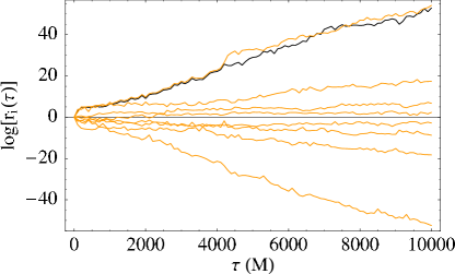
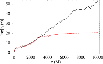
(a)		(b)

Figure 7: Natural logarithms of the phase space ellipsoid axes vs. proper time in Kerr spacetime with $S=1$. The slopes of the lines are the Lyapunov exponents; the largest exponent is approximately $\lambda_{\mathrm{max}}=5\times 10^{-3}\,M^{-1}$. The initial conditions are the same as in Fig. 6, and one point is recorded at each time $T=100\,M$ (Sec. III.2.1). (a) Full Gram-Schmidt Jacobian method (light) with rigorous Jacobian method (dark). The full GS method is rescaled at each time $T$ according the algorithm in Sec. III.2, while the rigorous Jacobian method is unrescaled. The two methods agree closely on the value of the largest Lyapunov exponent. (b) Rigorous Jacobian method compared to unrescaled deviation vector method. Note that the latter method, which started with a deviation of size $10^{-7}$, saturates at $\sim\!\!16$. This corresponds to a growth of $e^{16}\approx 9\times 10^{6}$, which means that the separation has grown to a size of order unity.

The numerical values of the exponents are shown in Table 1. The $\pm\lambda$ property is best satisfied by $\pm\lambda_{\rm max}$, the exponents with the largest absolute value. The exponents are least-squares fits to the data, with approximate standard errors of $1\%$. These errors are not particularly meaningful since the exponents themselves can vary by $\sim\!\!10\%$ depending on the initial direction of the deviation vector. Moreover, even exponents that appear nonzero may be indistinguishable from zero in the sense of Fig. 8; for such exponents a “$1\%$” error on the fit is meaningless.

For initial conditions considered in Fig. 6, and other orbits in the strongly relativistic region near the horizon, typical largest Lyapunov exponents are on the order of a ${\rm few}\times 10^{-3}/M$. For the particular case illustrated in Fig. 6, we have $\lambda_{\rm max}\approx 5\times 10^{-3}\,M^{-1}$, which implies an $e$-folding timescale of $\tau_{\lambda}\equiv 1/\lambda\approx 2\times 10^{2}\,M$. This is strongly chaotic, with a significant divergence in approximately eight $\phi$-orbital periods.

Based on integrations in the case of zero spin, which corresponds to no chaos (Lyapunov exponents all zero), we can determine how quickly the exponents approach zero numerically. Fig. 8 compares the four apparently positive exponents with a known zero exponent. Only two of the four exponents are unambiguously distinguishable from zero, consistent with the argument in Sec. VI.2 that there should be at most three independent nonzero exponents.

Finally, we note that the components of the direction of largest stretching are all nonzero in general. The chaos is not confined to the spin variables alone, but rather mixes all directions. This indicates that chaos could in principle manifest itself in the gravitational waves from extreme mass-ratio binaries—but see Sec. VII.3 below.

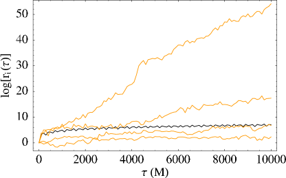
Figure 8: Ellipsoid axis lengths from the upper half of Fig. 7(a) (light), compared to an integration with zero spin and hence zero Lyapunov exponent (dark). Only two of the four lines represent exponents distinguishable from zero.

Table 1: Lyapunov exponents in Kerr spacetime in units of $10^{-3}\,M^{-1}$, using a least squares fit. The exponents correspond to the semimajor axis evolution shown in Fig. 7(a). As is typical with the Gram-Schmidt Jacobian method, the exponents with the largest magnitudes are determined most accurately, and thus show the $\pm\lambda$ property most clearly. The standard errors on the fit are $\sim\!\!1\%$ for each exponent, but these errors are dominated by two systematic errors: (1) the variation due to different choices of initial (random) tangent vectors; (2) nonzero numerical values even for exponents that converge to zero eventually. In particular, the four smallest exponents (in absolute value) are indistinguishable from zero (see Fig. 8).

$+\lambda$	$5.5$	$1.5$	$0.56$	$0.25$
$-\lambda$	$5.3$	$1.6$	$0.76$	$0.072$

VII.1.2 Schwarzschild spacetime revisited

We now reconsider the case of a spin $S=1$ particle in Schwarzschild spacetime, as investigated in Ref. (Suzuki and Maeda, 1997). Fig. 9 shows an orbit similar to a chaotic orbit considered there (Fig. 4(d) in (Suzuki and Maeda, 1997)). A plot of $\log[r_{i}(\tau)]$ vs. $\tau$ (Fig. 10) shows behavior similar to that in Fig. 7. In particular, the $\pm\lambda$ symmetry is present, apparently with two positive exponents. (The other lines are indistinguishable from zero, again using $S=0$ orbits as a baseline.) The largest exponent of $1.5\times 10^{-3}\,M^{-1}$ agrees closely with the value from Ref. (Suzuki and Maeda, 1997), which reported an exponent of $\sim\!\!2\times 10^{-3}\,M^{-1}$ for a similar orbit. (This agreement is somewhat surprising, since Suzuki and Maeda (1997) appears not to have taken the constrained nature of the deviation vectors into account. Luckily, the exponents are robust, and even unconstrained deviation vectors give nearly correct results.)

(a)		(b)

Figure 9: The orbit of a maximally spinning ($S=1$) test particle in Schwarzschild spacetime for $E=0.94738162\,\mu$ and $J_{z}=4.0\,\mu M$ As before, we plot (a)  $y$ vs. $x$ and (b) $z$ vs. $\rho=\sqrt{x^{2}+y^{2}}$.

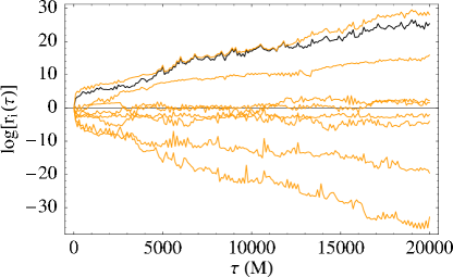
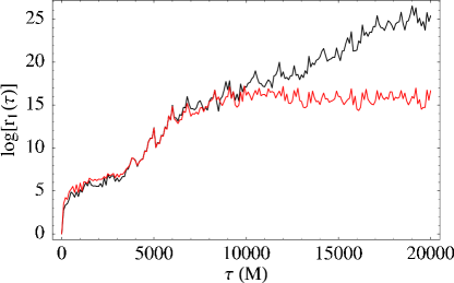
(a)		(b)

Figure 10: Natural logarithms of the phase space ellipsoid axes vs. proper time in Schwarzschild spacetime with $S=1$. The largest exponent is $\lambda_{\mathrm{max}}\approx 1.2\times 10^{-3}\,M^{-1}$. The initial conditions are the same as in Fig. 9. (a) Full Gram-Schmidt Jacobian method (light) with rigorous Jacobian method (dark). (b) Rigorous Jacobian method compared to unrescaled deviation vector method. As in Fig. 7(b), the unrescaled method eventually saturates.

Table 2: Lyapunov exponents in Schwarzschild spacetime in units of $10^{-3}\,M^{-1}$, using a least squares fit. The exponents correspond to the semimajor axis evolution shown in Fig. 10(a), which is similar to the orbit in Fig. 4(d) of Ref. (Suzuki and Maeda, 1997). As with the Kerr case (Table 1), the standard errors on the fit are $\sim\!\!1\%$ for each exponent, and the same caveats apply. The four smallest exponents (in absolute vale) are indistinguishable from zero in the sense of Fig. 8.

$+\lambda$	$1.2$	$0.67$	$0.21$	$0.0063$
$-\lambda$	$1.5$	$0.57$	$0.10$	$0.00023$

VII.1.3 Kerr and Schwarzschild compared

The Kerr and Schwarzschild Lyapunov exponents of the previous two sections are not all that different; both are $10^{-2}$–$10^{-3}\,M^{-1}$ in order of magnitude. Nevertheless, the two systems prove to be quite different: chaotic orbits are easy to find in Kerr spacetime for nearly any initial condition that explores the strongly relativistic region near the horizon, whereas nearly all analogous orbits in Schwarzschild spacetime are not chaotic.

Fig. 11 compares Kerr and Schwarzschild orbits with the same inclination angle $\iota=10^{\circ}$ and eccentricity $e=0.5$ but varying pericenters $r_{p}$. (Details of this parameterization method, mentioned above in Sec. II.3, appear in (Hartl_2_2002).) We insure that the systems are analogous by using orbits of $S=1$ particles with the same values of $r_{p}/r_{\mathrm{ms}}$, where $r_{\mathrm{ms}}$ is the radius of the marginally stable orbit in the corresponding $S=0$ (geodesic) case. We use a Kerr geodesic integrator developed by Scott Hughes (Hughes, ) to find $r_{\mathrm{ms}}$, which is the smallest pericenter that still yields a stable orbit. For the values of $\iota$ and $e$ considered, $r_{\mathrm{ms}}=1.0\,M$ for Kerr and $r_{\mathrm{ms}}=4.67\,M$ for Schwarzschild.

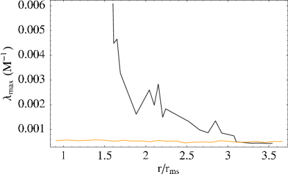
Figure 11: Comparison of maximally spinning ($S=1$) particle orbits in Kerr (dark) and Schwarzschild (light). We plot the largest Lyapunov exponent versus pericenter (normalized by the marginally stable radius). The Kerr initial conditions for the innermost orbits are essentially as in Fig. 6. The Schwarzschild orbits are identical to their Kerr counterparts in inclination ($10^{\circ}$) and eccentricity ($e=0.5$) but have the Kerr parameter $a$ set to zero. The Schwarzschild orbits have exponents indistinguishable from zero over the entire range of parameters.

It is evident from Fig. 11 that the Kerr orbits are chaotic for a broad range of pericenters, with the maximum Lyapunov $\lambda_{\mathrm{max}}$ generally decreasing as the pericenter increases. In contrast, the Schwarzschild orbits are not chaotic anywhere over the entire range of valid initial conditions. In fact, we are unable to find any chaotic orbits in Schwarzschild spacetime other than the types identified by Suzuki and Maeda Suzuki and Maeda (1997), which were exceptional cases of orbits on the edge of a generalized effective potential. In Kerr, on the other hand, chaotic orbits appear to be the rule for pericenters near $r_{\mathrm{ms}}$.

VII.2 Dependence on $S$

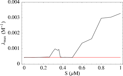
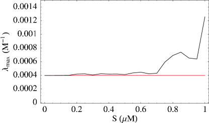
(a)		(b)

Figure 12: Variation of largest Lyapunov exponent vs. $S$. (a) The spin $S=1$ initial conditions are the same as in Fig. 6. (b) Another $S=1$ case with a different inclination angle ($20^{\circ}$) and pericenter ($2.5\,M$). As the spin decreases, we hold fixed the Kerr orbital parameters: inclination angle, eccentricity, and pericenter. Note that in (a) the chaos disappears below $S\sim 0.5$, but returns in a region centered on $S\sim 0.3$. The horizontal line in both plots is the value of $\lambda_{\mathrm{max}}$ calculated for the baseline $S=0$ orbit. In both (a) and (b) the Lyapunov exponent is indistinguishable from zero for physically realistic spins.

Since chaos must disappear as $S\rightarrow 0$, we expect to see the largest Lyapunov exponent approach zero in this limit. This is indeed the case: in Fig. 12, which shows the variation of $\lambda_{\mathrm{max}}$ with $S$ for two different orbits, we see that the chaos unambiguously present when $S=1$ is not present for smaller values of $S$. In particular, the largest Lyapunov exponent is indistinguishable from zero over the entire range $10^{-6}\leq S\leq 10^{-1}$. (The far left of the plots have data points for each decade in this range.)

Although the strength of the chaos generally decreases with $S$, one remarkable feature of Fig. 12(a) is the return of chaotic orbits between $S\sim 0.25$ and $0.4$ after their disappearance at $S\sim 0.5$. The effect is qualitatively clear in Fig. 13. This chaotic “bump” in $\lambda_{\mathrm{max}}$ vs. $S$ illustrates an important theme in nonlinear dynamical systems: the only way to determine whether an orbit is chaotic is to do the calculation. Though we certainly expect the strength of chaos to be smaller for $S\ll 1$ than for $S\approx 1$, it is impossible, in general, to determine a priori whether a particular set of parameters will lead to chaotic behavior.

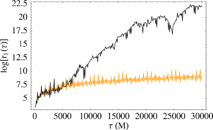
Figure 13: Two orbits from the “bump” in Fig. 12(a). The $S=0.4$ orbit (light) is not chaotic, but the $S=0.3$ orbit (dark) is chaotic, despite having a smaller value of the spin.

VII.3 Physically realistic spins

The Papapetrou equations are only realistic in the test-particle limit, so physically realistic spins must satisfy $S\ll 1$ (Sec. II.2). This corresponds to likely sources of gravitational waves for LISA (Finn and Thorne, 2000; Hughes, 2000, 2001b), e.g., maximally spinning $\mu=10\,M_{\odot}$ black holes spiraling into supermassive $M=10^{6}\,M_{\odot}$ Kerr black holes, which have spin parameters of $S=\mu/M=10^{-5}$. Because of their likely importance as emitters of gravitational waves, it is essential to understand the dynamics of such systems.

VII.3.1 Vanishing Lyapunov exponents

We would like to be able to make a definitive statement about the presence or absence of chaos for “small” spins, e.g., values of $S$ in the range $10^{-2}$–$10^{-6}$. Unfortunately, when determining Lyapunov exponents numerically, it is impossible to conclude definitively that an orbit is or is not chaotic, since to do so would require an infinite-time integration. On the other hand, for suspected non-chaotic orbits, we can provide an approximate bound on the $e$-folding timescale.

Figure 14: The variation of the dimensionless quantity $\lambda_{\mathrm{max}}\,M$ with final integration time $\tau_{f}$ for spin parameter $S$ in the range $10^{-2}\leq S\leq 10^{-6}$. From top to bottom, the total integration time varies from $10^{4}\,M$ to $10^{7}\,M$. It is likely that the true Lyapunov exponent is zero.

The numerical values of exponents suspected to be zero depend strongly on the time of the integration. For example, for values of $S$ in the range $10^{-2}\leq S\leq 10^{-6}$, the exponent in Fig. 12 appears to be $\lambda_{\mathrm{max}}\approx 5\times 10^{-4}\,M^{-1}$, but this plot represents an integration time of only $10^{4}\,M$. Longer integration times give correspondingly smaller estimates for the suspected zero exponents (Fig. 14). For the system shown in Fig. 12, an integration of $10^{7}\,M$ yields an estimate of $\lambda_{\mathrm{max}}\approx 3.0\times 10^{-7}\,M^{-1}$ for all spins in the range $10^{-2}\leq S\leq 10^{-7}$. In this case, the relevant Lyapunov timescales are at least $3\times 10^{6}\,M$, and are probably much longer; the size of the bound is limited only by our patience and computer budget. It seems highly likely that such orbits are not chaotic.

VII.3.2 Spin-induced phase differences

Table 3: Phase shifts $\Delta\phi=\phi_{\mathrm{geodesic}}-\phi_{\mathrm{spin}}$ in radians as a function of orbital inclination angle $\iota$ and pericenter $r_{p}$ for $a=0.5$ and $S=10^{-5}$. Inclination angle $\iota=0^{\circ}$ is prograde equatorial and $\iota=180^{\circ}$ is retrograde equatorial. The geodesic orbits and their corresponding spin orbits start with the same initial 4-velocity $v^{\mu}$, and the integrations are performed using Boyer-Lindquist coordinate time $t$, with $t_{\mathrm{max}}\approx$ (2000 times the average radial orbital period). The pericenters are scaled by the marginally stable radius $r_{\mathrm{ms}}$, and we start at $r_{p}/r_{\mathrm{ms}}=1.5$ to guarantee the existence of valid initial conditions for the non-geodesic orbit. The spin has fixed initial values of $S^{\hat{r}}=S^{\hat{\mu}}=0.1\,S$ (with hats indicating an orthonormal basis), corresponding to initial angles of $9^{\circ}$ to $30^{\circ}$ with respect to the vertical in the particle’s rest frame, increasing with decreasing pericenter.

$r_{p}/r_{\mathrm{ms}}$
$\iota$	1.5	2.0	2.5	3.0	3.5	4.0	4.5	5
$10^{\circ}$	1.50e-02	5.69e-03	4.32e-03	2.13e-03	2.02e-03	1.27e-03	1.14e-03	7.77e-04
$45^{\circ}$	2.79e-02	1.23e-02	1.01e-02	4.34e-03	4.60e-03	2.24e-03	1.66e-03	1.83e-03
$85^{\circ}$	4.36e-02	2.92e-03	1.48e-03	8.24e-04	1.00e-03	2.20e-03	1.86e-03	1.26e-03
$135^{\circ}$	-9.02e-03	-6.25e-03	-2.34e-03	-1.30e-03	-1.73e-03	-8.17e-04	-6.76e-04	-7.72e-04
$170^{\circ}$	8.40e-04	2.85e-04	1.84e-04	7.31e-05	1.25e-04	1.12e-04	3.35e-05	3.07e-05

Table 4: Phase shifts $\Delta\phi=\phi_{\mathrm{geodesic}}-\phi_{\mathrm{spin}}$ in radians as a function of orbital inclination angle $\iota$ and pericenter $r_{p}$ for $a=1$ and $S=10^{-5}$. As in Table 3, the pericenters are scaled by $r_{\mathrm{ms}}$, and the spin has fixed initial values of $S^{\hat{r}}=S^{\hat{\mu}}=0.1\,S$ (corresponding in this case to initial angles of $28^{\circ}$ to $61^{\circ}$, again decreasing with increasing pericenter).

$r_{p}/r_{\mathrm{ms}}$
$\iota$	1.5	2.0	2.5	3.0	3.5	4.0	4.5	5
$10^{\circ}$	7.21e-02	4.58e-02	2.41e-02	1.83e-02	1.10e-02	9.46e-03	6.56e-03	7.43e-03
$45^{\circ}$	2.37e-01	5.56e-02	2.59e-02	1.83e-02	1.73e-02	1.52e-02	1.08e-02	7.83e-03
$85^{\circ}$	1.96e-02	6.21e-03	2.82e-03	2.13e-03	2.66e-02	3.64e-03	6.47e-04	3.48e-03
$135^{\circ}$	-1.04e-02	-3.17e-03	-3.21e-03	-1.41e-03	-1.12e-03	-8.46e-04	-8.82e-04	-5.59e-04
$170^{\circ}$	3.89e-04	1.48e-04	6.68e-05	5.97e-05	8.09e-05	9.55e-05	3.06e-05	1.66e-05

Even if their Lyapunov exponents are zero, small spins affect the relative phase of the orbits, and since phase differences accumulate secularly (Apostolatos et al., 1994), the spin can still affect the gravitational wave signal. It is therefore useful to have a sense of the orders of magnitude of such spin-induced phase-shifts. Tables 3 and 4 show typical values for the phase difference $\Delta\phi=\phi_{\mathrm{geodesic}}-\phi_{\mathrm{spin}}$ for $S=10^{-5}$, where the geodesic and spin systems start with the same initial 4-velocity $v^{\mu}$. The most useful quantity in practice is the phase shift as measured by observers at infinity, so we integrate in terms of the Boyer-Lindquist coordinate time $t$ in place of $\tau$. (This involves multiplying the differential equations by $d\tau/dt$ at each time step.) As is apparent from the tables, the phase shifts range broadly, from  $10^{-1}$ to $10^{-5}$ radians after 2000 radial orbital periods, but tend to decrease in magnitude with increasing inclination angle or pericenter.

Ref. Hughes (2001b) shows that the number of orbital periods in a full inspiral from $r\approx 4\,M$ to the final plunge is $N\sim\frac{M}{\mu}$, which is $10^{5}$ for the systems in Tables 3 and 4. Since the table represents values of $\Delta\phi$ for $2000$ times the average radial orbital period, this means that the total phase shift during the inspiral is $50\,\Delta\phi_{\mathrm{table}}$. For a $10^{\circ}$ inclination angle the total phase shift is on the order of a tenth of a radian to a radian. Slightly more realistic values of the number of orbits can be obtained using Fig. 2 in Hughes (2001b), which gives $N\sim 2\times 10^{4}$ orbital periods from $r=4\,M$ to the plunge at $r\approx M$ for $a=0.998$, $\iota=10^{\circ}$, and $M/\mu=10^{5}$. Since the orbit spends most of its time between $4\,r_{\mathrm{ms}}$ and $2\,r_{\mathrm{ms}}$, interpolating in Table 4 gives $\Delta\phi_{\mathrm{total}}\approx 10\times\Delta\phi_{r=3.0}=2\times 10^{-2}$. This is only a rough estimate, since the orbits in Hughes (2001b) are circular, while the orbits we consider are eccentric.

VII.4 Comments on time, rescaling, and norms

In this paper, we have elected to use $\tau$ as the time parameter, a rescaling time $T$ of $100\,M$, and a projected norm (Sec. IV.1). Here we discuss the effects of varying these choices.

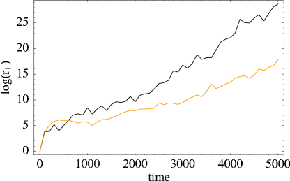
Figure 15: The natural logarithm of the largest ellipsoid axis vs. time for proper time $\tau$ (dark) and coordinate time $t$ (light). The exponents are clearly different, but the Lyapunov timescales $\tau_{\lambda}=1/\lambda_{\tau}$ and $t_{\lambda}=1/\lambda_{t}$ are related by Eq. (56).

First, we consider the effects of using coordinate time $t$ in place of $\tau$. In Fig. 15, we plot the natural logarithm of the largest ellipsoid axis $\log[r_{1}(\tau)]$ vs. $\tau$ together with $\log[r_{1}(t)]$ vs. $t$. (We use the unrescaled deviation vector approach for simplicity, since the Jacobian approach requires a new Jacobian matrix for each coordinate change.) The exponents are $\lambda_{\tau}=5.05\times 10^{-3}\,M^{-1}$ and $\lambda_{t}=2.51\times 10^{-3}\,M^{-1}$, implying Lyapunov timescales of $\tau_{\lambda}=1.98\times 10^{2}\,M$ and $t_{\lambda}=3.98\times 10^{2}\,M$. The average value of $dt/d\tau$ over the orbit is 2.06, whereas $t_{\lambda}/\tau_{\lambda}=2.01$, so the relationship

$$\frac{t_{\lambda}}{\tau_{\lambda}}=\left\langle\frac{dt}{d\tau}\right\rangle$$ (56)

discussed in the introduction is well satisfied.

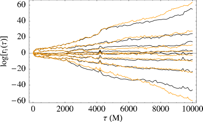
Figure 16: Natural logarithms of the ellipsoid axes vs. $\tau$ for rescaling time $T=100\,M$ (dark) and time $T=50\,M$ (light).

Second, we discuss the effects of varying the rescaling time $T$. We find that choosing $T$ to be a moderate fraction of the shortest Lyapunov timescale (corresponding to the largest Lyapunov exponent) works best, giving each axis enough time to grow before rescaling while still keeping the negative exponents from underflowing and preventing the largest axis from dominating. Rescaling times between $50\,M$ and $100\,M$ work best for the systems we consider, which have Lyapunov timescales ranging from $10^{2}\,M$ to $10^{3}\,M$. A comparison of results for $T=50\,M$ and $T=100\,M$ appears in Fig. 16.

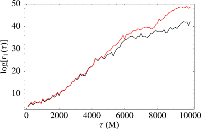
Figure 17: The natural logarithm of the largest ellipsoid axis vs. $\tau$ for the Euclidean norm (top) and the projected norm from Sec. IV.1 (bottom).

Third, we compare the projected norm used here to a naive Euclidean norm for determining the length of the phase-space tangent vectors $\bm{\xi}_{i}$. As shown in Fig. 17, even using a 12-dimensional Euclidean norm changes the resulting exponent very little (approximately 15% in this example). Given its conceptual advantages, we choose to use the projected norm with the confidence that the Lyapunov exponent order of magnitude is robust.

VIII Conclusions

A spinning test particle, as described by the Papapetrou equations, appears to be chaotic in Kerr spacetime, with maximum $e$-folding timescales of a $\textrm{few}\times 10^{2}\,M$. The applicability of this result is limited by three main factors: (1) chaos appears only for physically unrealistic values of the spin parameter; (2) other effects, such as tidal coupling, may be important for some astrophysical systems, violating the pole-dipole approximation implicit in the Papapetrou equations; and (3) we neglect gravitational radiation. The third limitation is not fatal, since the radiation timescales can be long enough that chaos, if present in the conservative limit, would have time to manifest itself in the gravitational radiation of extreme mass-ratio systems.

In the unphysical $S=1$ limit, the Lyapunov exponents exhibit characteristics expected of a Hamiltonian system, appearing in pairs $\pm\lambda$ (Sec. VI.2). There are zero Lyapunov exponents which correspond to the constants of the motion, but the other exponents are in general nonzero. (For the Kerr orbits considered in this paper, we find that two of the three independent exponents are nonzero, as illustrated in Fig. 8.) Typical orders of magnitude for the largest Lyapunov exponents are a $\textrm{few}\times 10^{-3}\,M^{-1}$ for unphysical spins ($S=1$). For physically realistic spin parameters (Sec. VII.3), we find that $\lambda_{\mathrm{max}}\lesssim\textrm{few}\times 10^{-7}\,M^{-1}$, corresponding to $e$-folding timescales of a $\textrm{few}\times 10^{6}\,M$. Even this bound appears to be limited only by the total integration time; in all physically realistic cases considered, $\lambda_{\mathrm{max}}$ is indistinguishable from zero (using $S=0$ integrations as a baseline).

From the perspective of gravitational radiation detection, our most important conclusion is that chaos seems to disappear for physically realistic values of $S$, i.e., values of $S$ for which the test-particle approximation and hence the Papapetrou equations are valid. We are unable to comment on the dynamics of comparable mass-ratio binaries, since such systems are not accurately modeled by the Papapetrou equations, but for extreme mass-ratio binaries it appears unlikely that chaos will present a problem for the calculation of theoretical templates for use in matched filters. A more thorough exploration of parameter space is needed to reach a firmer conclusion (Hartl_2_2002).

*

Appendix A Full Jacobian

For reference, we list the derivatives needed to calculate the full Jacobian matrix.

From Sec. V.2, we have the following:

$$\frac{\partial\dot{x}^{\mu}}{\partial x^{\nu}} = N\left[p_{\alpha}g^{\alpha\mu}_{\ \ ,\nu}+w^{\mu}_{\ ,\nu}\right.$$ (57)

$$\left.+\,v^{\mu}(v_{\alpha}w^{\alpha}_{\ ,\nu}+\textstyle{1\over 2}Nw^{\alpha}w^{\beta}g_{\alpha\beta,\nu})\right]$$

$$\frac{\partial\dot{x}^{\mu}}{\partial p_{\nu}}=N(g^{\mu\nu}+W^{\mu\nu}+Nv^{\mu}w^{\nu})+Nv^{\mu}v_{\alpha}W^{\alpha\nu}$$ (58)

with

$$W^{\mu\nu}=-{{}^{*}}R^{*\mu\alpha\nu\beta}_{\ \ \ \ \ }S_{\alpha}S_{\beta}$$ (59)

$$\frac{\partial\dot{x}^{\mu}}{\partial S_{\nu}}=NV^{\mu\nu}+Nv^{\mu}v_{\alpha}V^{\alpha\nu}$$ (60)

with

$$V^{\mu\nu}=-S_{\alpha}p_{\beta}({{}^{*}}R^{*\mu\alpha\beta\nu}-{{}^{*}}R^{*\mu\nu\alpha\beta})$$ (61)

Now we simply apply the product rule many times:

$$\frac{\partial\dot{p}_{\mu}}{\partial x^{\nu}} = -p_{\alpha}S_{\beta}\left(R^{*\ \ \alpha\beta}_{\mu\gamma\ \ \ ,\nu}\,v^{\gamma}+R^{*\ \ \alpha\beta}_{\mu\gamma}\,v^{\gamma}_{\ ,\nu}\right)$$ (62)

$$+\,p_{\alpha}\left(\Gamma^{\alpha}_{\ \beta\mu,\nu}\,v^{\beta}+\Gamma^{\alpha}_{\ \beta\mu}\,v^{\beta}_{\ ,\nu}\right)$$

$$\frac{\partial\dot{p}_{\mu}}{\partial p_{\nu}} = -S_{\beta}\left(R^{*\ \ \nu\beta}_{\mu\gamma\ \ }\,v^{\gamma}+R^{*\ \ \alpha\beta}_{\mu\gamma}\,p_{\alpha}\frac{\partial v^{\gamma}}{\partial p_{\nu}}\right)$$ (63)

$$+\,\Gamma^{\nu}_{\ \beta\mu}\,v^{\beta}+\Gamma^{\alpha}_{\ \beta\mu}\,p_{\alpha}\frac{\partial v^{\beta}}{\partial p_{\nu}}$$

$$\frac{\partial\dot{p}_{\mu}}{\partial S_{\nu}} = -R^{*\ \ \alpha\nu}_{\mu\gamma\ \ }\,v^{\gamma}p_{\alpha}-R^{*\ \ \alpha\beta}_{\mu\gamma}\frac{\partial v^{\gamma}}{\partial S_{\nu}}p_{\alpha}S_{\beta}$$ (64)

$$+\,\Gamma^{\alpha}_{\ \beta\mu}\,p_{\alpha}\frac{\partial v^{\beta}}{\partial S_{\nu}}$$

$$\frac{\partial\dot{S}_{\mu}}{\partial x^{\nu}} = -p_{\mu}S_{\alpha}p_{\gamma}S_{\delta}\left(R^{*\alpha\ \gamma\delta}_{\ \ \beta\ \ \ ,\nu}\,v^{\beta}+R^{*\alpha\ \gamma\delta}_{\ \ \beta}\,v^{\beta}_{\ ,\nu}\right)$$ (65)

$$+\,S_{\alpha}\left(\Gamma^{\alpha}_{\ \beta\mu,\nu}\,v^{\beta}+\Gamma^{\alpha}_{\ \beta\mu}\,v^{\beta}_{\ ,\nu}\right)$$

$$\frac{\partial\dot{S}_{\mu}}{\partial p_{\nu}} = -S_{\alpha}S_{\delta}v^{\beta}\left(\delta_{\mu}^{\ \nu}R^{*\alpha\ \gamma\delta}_{\ \ \beta}\,p_{\gamma}\,+p_{\mu}R^{*\alpha\ \nu\delta}_{\ \ \beta}\right)$$ (66)

$$-\,p_{\mu}R^{*\alpha\ \gamma\delta}_{\ \ \beta}S_{\alpha}\frac{\partial v^{\beta}}{\partial p_{\nu}}p_{\gamma}S_{\delta}$$

$$+\,\Gamma^{\alpha}_{\ \beta\mu}\,\frac{\partial v^{\beta}}{\partial p_{\nu}}S_{\alpha}$$

$$\frac{\partial\dot{S}_{\mu}}{\partial S_{\nu}} = -p_{\mu}p_{\gamma}v^{\beta}\left(R^{*\nu\ \gamma\delta}_{\ \ \beta}\,S_{\delta}+R^{*\alpha\ \gamma\nu}_{\ \ \beta}\,S_{\alpha}\right)$$ (67)

$$-\,p_{\mu}R^{*\alpha\ \gamma\delta}_{\ \ \beta}S_{\alpha}\frac{\partial v^{\beta}}{\partial S_{\nu}}p_{\gamma}S_{\delta}$$

$$+\,\Gamma^{\nu}_{\ \beta\mu}\,v^{\beta}+\Gamma^{\alpha}_{\ \beta\mu}\,\frac{\partial v^{\beta}}{\partial S_{\nu}}S_{\alpha}$$

Accidentally leaving off the final term in $\displaystyle{\frac{\partial\dot{S}_{\mu}}{\partial S_{\nu}}}$ led to the robust but spurious chaotic behavior mentioned in Sec. V.1.

References

- Levin (2000) J. Levin, Phys. Rev. Lett. 84, 3515 (2000).
- (2) J. Levin, eprint gr-qc/0010100.
- Suzuki and Maeda (1997) S. Suzuki and K. Maeda, Phys. Rev. D 55, 4848 (1997).
- Schnittman and Rasio (2001) J. D. Schnittman and F. A. Rasio, Phys. Rev. Lett. 87, 121101 (2001).
- Cornish (2001) N. J. Cornish, Phys. Rev. D 64, 084011 (2001).
- (6) N. J. Cornish and J. Levin, eprint gr-qc/0207016.
- Cornish and Levin (2002) N. J. Cornish and J. Levin, Phys. Rev. Lett. 89, 179001 (2002).
- Hughes (2001a) S. A. Hughes, Class. Quantum Grav. 18, 4067 (2001a).
- (9) See http://lisa.jpl.nasa.gov.
- Alligood et al. (1997) K. T. Alligood, T. D. Sauer, and J. A. Yorke, Chaos: An Introduction to Dynamical Systems (Springer, New York, 1997).
- Cornish and Levin (1997) N. Cornish and J. Levin, Phys. Rev. Lett. 78, 998 (1997).
- Ott (1993) E. Ott, Chaos in Dynamical Systems (Cambridge University Press, Cambridge, England, 1993).
- Misner et al. (1973) C. W. Misner, K. S. Thorne, and J. A. Wheeler, Gravitation (Freeman, San Francisco, 1973).
- Papapetrou (1951) A. Papapetrou, Proc. R. Soc. London A209, 248 (1951).
- Dixon (1970) W. G. Dixon, Proc. R. Soc. London A314, 499 (1970).
- Møller (1972) C. Møller, Theory of Relativity (Oxford University Press, London, 1972).
- Barker and O’Connell (1974) B. M. Barker and R. F. O’Connell, Gen. Relativ. Gravit. 5, 539 (1974).
- Kidder (1995) L. E. Kidder, Phys. Rev. D 52, 821 (1995).
- Semerák (1999) O. Semerák, Mon. Not. R. Astron. Soc. 308, 863 (1999).
- Cook et al. (1994) G. B. Cook, S. L. Shapiro, and S. A. Teukolsky, Astrophys. J. 424, 823 (1994).
- Lai et al. (1993) D. Lai, F. A. Rasio, and S. L. Shapiro, Astrophys. J. Suppl. Ser. 88, 205 (1993).
- Nauenberg (1972) M. Nauenberg, Astrophys. J. 175, 417 (1972).
- Geroyannis and Papasotiriou (2000) V. S. Geroyannis and P. J. Papasotiriou, Astrophys. J. 534, 359 (2000).
- Wiggins and Lai (2000) P. Wiggins and D. Lai, Astrophys. J. 532, 530 (2000).
- Tanaka et al. (1996) T. Tanaka, Y. Mino, M. Sasaki, and M. Shibata, Phys. Rev. D 54, 3762 (1996).
- Eckmann and Ruelle (1985) J.-P. Eckmann and D. Ruelle, Rev. Mod. Phys. 57, 617 (1985).
- Karas and Vokrouhlický (1992) V. Karas and D. Vokrouhlický, Gen. Relativ. and Grav. 24, 729 (1992).
- Press et al. (1992) W. H. Press, S. A. Teukolsky, W. T. Vetterling, and B. P. Flannery, Numerical Recipes in C (Cambridge University Press, Cambridge, England, 1992).
- Binney and Tremaine (1987) J. Binney and S. Tremaine, Galactic Dynamics (Princeton University Press, Princeton, NJ, 1987).
- Hojman (1975) S. Hojman, Ph.D. thesis, Princeton University (1975).
- Dirac (1964) P. A. M. Dirac, Lectures on Quantum Mechanics (Belfer Graduate School of Science, Yeshiva University, New York, 1964).
- Hanson and Regge (1974) A. J. Hanson and T. Regge, Ann. Phys. (N.Y.) 87, 498 (1974).
-
(33)
S. Hughes, http://www.tapir.caltech.edu/
in listwg1/EMRI/hughes_geodesic.html. - Finn and Thorne (2000) L. S. Finn and K. S. Thorne, Phys. Rev. D 62, 124021 (2000).
- Hughes (2000) S. A. Hughes, Phys. Rev. D 61, 084004 (2000).
- Hughes (2001b) S. A. Hughes, Phys. Rev. D 64, 064004 (2001b).
- Apostolatos et al. (1994) T. A. Apostolatos, C. Cutler, G. J. Sussman, and K. S. Thorne, Phys. Rev. D 49, 6274 (1994).