Waves in Schwarzschild spacetimes: how strong can be imprints of the spacetime curvature

Abstract

Emitted radiation can be reprocessed in curved spacetimes, due to the breakdown of the Huyghens principle. A maximization procedure for the energy diffusion allows one to obtain wave packets (gravitational and electromagnetic) that are particularly strongly backscattered. Examples are shown with the backscattered part exceeding by one order remnants of initial signals. A robust ringing can be observed, with amplitudes exceeding leftovers of the main radiation pulse. The analysis of the obtained results allows one to set demands on some parameters in the numerical description of a realistic process of the collapse of two black holes.

I Introduction

It is known essentially since the times of Hadamard [1] that curved spacetimes can affect the propagation of waves. The breakdown of the Huyghens principle [1] (or the backscatter, a name adopted by the general relativity community after de Witt and Brehme [2]) can influence both the energy and the energy flux of a wave signal. The backscatter can leave its imprints on the frequency spectrum and can affect the transmission time. The manifestations of this effect are the so-called tails and, most impressively, the quasinormal modes (QNM thereafter). The literature on the backscattering and related phenomena is quite extensive – see ([3] – [23]) and numerous references therein.

The QNM’s have some features of the scattering-type solutions and they have been studied in the context of general relativity for more than three decades [6]. Many of their characteristics are well known for black holes [14], for instance their (complex) frequency spectrum. An observer located at a fixed space position would find that QNM’s oscillate with amplitudes decreasing exponentially in time. The oscillation periods and the damping exponents are the real and the imaginary parts of a frequency, respectively. They depend only on a few global characteristics of black holes – their asymptotic mass, angular momentum and/or global electric charge. Therefore their identification in an observed wave spectrum would unambiguously identify a black hole (and in fact provide an argument, closest to the direct observation, in favour of the existence of black holes). Extensive reviews are presented in [20] and [21]. Tail terms have been studied in 1970’s beginning from Price [8] but interest in them has again revived recently [23].

The spectra of QNM’s and the decay exponents of the tails are universal, independent of initial data, but the very existence of QNM’s and their amplitudes (as well of the tails) do depend on initial wave conditions. The main aim of this paper is to show the strongest imprints of the spacetime curvature that are present in the form of QNM’s in a propagating wave. The implementation of this task requires the separation of the genuine geometric effects from those being built into initial data – notice that even in the Minkowski spacetime one can easily form a QNM-like structure by producing suitable initial data. The simplest possibility is to consider the purely backscattered part of the initial radiation, which is absent in the Minkowski geometry but which always exists in a curved spacetime.

It would be meaningless to try to accomplish our aim by the method of ”trial and error” – by selecting at random various initial wave configurations from the ocean of all possible data. Rather one should focus on “extremal” in some sense initial data that can generate, in the first instance, “extremal” asymptotic templates, but also can set bounds on some parameters used in the numerical descriptions. In the present paper we follow the second strategy, using as a guiding principle the idea of extremizing the so-called diffusion parameter [24] and addressing following issues. First, we estimate the maximal strength of the backscatter. The corresponding profiles of initial wave packets are found to favour vigorous ringing and/or strong deformation of initial signals. Second, and in relation with the former point, we obtain information on the process of taking waveforms from specific properties of the backscattered radiation. The order of the rest of this paper is as follows. Sec. 2 provides basic information on the wave equations. Sec. 3 describes in detail the procedure of maximizing the diffusion parameter and shows exemplary initial data for the wave evolution. Sec. 4 reviews some representative examples of wave templates. In Sec. 5 we again review those features of the numerical examples that could be useful for the numerical relativists dealing with the full nonlinear description of the collapse of two black holes. Sec. 6 summarizes main conclusions.

II Basic definitions and concepts

A Equations

The spacetime geometry is defined by the line element

$$ds^{2}=-\eta_{R}dt^{2}+{dR^{2}\over\eta_{R}}+R^{2}d\Omega^{2},$$ (1)

where $t$ is a time coordinate, $R$ is the radial areal coordinate, $\eta_{R}=1-{2m\over R}$ and $d\Omega^{2}=d\theta^{2}+\sin^{2}\theta d\phi^{2}$ is the line element on the unit sphere, $0\leq\phi<2\pi$ and $0\leq\theta\leq\pi$. Throughout this paper the Newtonian constant $G$ and the velocity of light $c$ are put equal to 1.

We will study the propagation of polar and axial modes of the quadrupole gravitational waves (GW thereafter) and the dipole electromagnetic waves (EW) in the Schwarzschild background. The evolution equation has the form

$$(-\partial_{t}^{2}+\partial_{r^{*}}^{2})\Psi=V\Psi.$$ (2)

Here $r^{*}=R+2m\ln\Bigl{(}{R\over 2m}-1\Bigr{)}$ is the tortoise coordinate while the potential term reads: for the polar GW

$$V(R)=6{\eta^{2}_{R}\over R^{2}}+\eta_{R}{63m^{2}(1+{m\over R})\over 2R^{4}(1+{3m\over 2R})^{2}};$$ (3)

for the axial GW

$$V(R)=6{\eta_{R}\over R^{2}}(1-{m\over R});$$ (4)

and for the dipole EW

$$V(R)=2{\eta_{R}\over R^{2}}.$$ (5)

The evolution equations corresponding to the first two potentials are called the Zerilli equation [25] and the Regge-Wheeler equation [26], respectively.

B Conserved energy

The equation (2) possesses a conserved energy,

$$E(R,t)=\int\limits_{R}^{\infty}{dr\over\eta_{r}}\Biggl{(}(\partial_{t}\Psi)^{2}+(\partial_{r^{*}}\Psi)^{2}+V\Psi^{2}\Biggr{)};$$ (6)

that is, the rate of change of $E$ in a fixed volume equals to the total flow through the boundary ([27] and [28]). This agrees (up to a constant factor) with the energy deduced from the stress-energy tensor for the EW. Eq. (6) represents a mathematically useful quantity in the case of the gravitational waves, with the density being asymptotically proportional to the density in the quadrupole formula. In either case, the energy conservation becomes important in our forthcoming construction.

Assume that initial data $\Psi$ and $\partial_{t}\Psi$ vanish inside a sphere having a radius $a>2m$. From the conservation law one easily finds that the amount of the energy that reaches a distant observer is equal to

$$E_{a}(\infty)\equiv E(a,t=0)-\delta E_{a},$$ (7)

where

$$\delta E_{a}=\int\limits_{0}^{\infty}dt\Biggl{(}(\partial_{t}\Psi+\partial_{r^{*}}\Psi)^{2}+V\Psi^{2}\Biggr{)}$$ (8)

([27] and [28]). The integration in (8) is done along the outgoing null cone that starts from $a$ at $t=0$. In the Minkowski spacetime (put formally $m=0$ in Eq. (2)) all of an initially outgoing radiation would get to infinity; in this case $\delta E_{a}=0$, since there is no diffusion through the null cone that expands outward from the initial position $R=a$. It is meaningful to distinguish between the momentarily outgoing and ingoing radiation also in a curved, but asymptotically flat, spacetime. One can give either an operational or an analytic definition. Imagine a directional wave generator that sends all radiation in a fixed direction, when located in an almost flat region. (That makes sense, since it is known from analytic estimates, that the fraction of the backscattered energy must fall off at least as $C\times(2m/a)^{2}$, where $C$ is of the order of unity – [27], [28] and [29]. By choosing a sufficiently distant location one can make the diffused energy $\delta E_{a}$ arbitrarily small.) This generator, when carefully moved to a strongly curved region, will preserve its property of generating directed radiation, which can be initially purely outgoing (or initially purely ingoing). Alternatively, one can work out an analytic definition. Initial data can always be split into two parts, one “initially outgoing” (defined below; in the Minkowski spacetime that would all get to the infinity) and the other purely ingoing (its form is similar to the former – just change $r^{*}-t$ into $r^{*}+t$ and some signs in the expansion – but it is purely ingoing in the Minkowski spacetime). We will show in Sec. 3, that the concept of initially outgoing waves is useful in bulding a nontrivial construction, and that fact in itself justifies this notion.

C Initial data for wave equations

Let us define

$$\tilde{\Psi}(R,t)=\Psi_{0}(r^{*}-t)+{\Psi_{1}(r^{*}-t)\over R}+{\Psi_{2}(r^{*}-t)\over R^{2}},$$ (9)

where $\Psi_{i}$’s ($i=0,1,2$) satisfy following relations:

$$\partial_{t}\Psi_{1}=3\Psi_{0},~{}~{}~{}~{}~{}~{}~{}~{}\partial_{t}\Psi_{2}=\Psi_{1}-m\partial_{t}\Psi_{1},$$ (10)

$$\partial_{t}\Psi_{1}=3\Psi_{0},~{}~{}~{}~{}~{}~{}~{}~{}\partial_{t}\Psi_{2}=\Psi_{1}-{m\over 2}\partial_{t}\Psi_{1},$$ (11)

$$\partial_{t}\Psi_{1}=\Psi_{0},~{}~{}~{}~{}~{}~{}~{}~{}~{}~{}~{}~{}\Psi_{2}=0,$$ (12)

for the polar GW, axial GW and dipole EW, respectively. In the Minkowski spacetime the function $\tilde{\Psi}$ exactly solves Eq. (2). We assume that $\tilde{\Psi}_{i}(r^{*},t=0)$’s vanish for $R\leq a$. Notice that only one of the three functions (for instance $\Psi_{0}$) can be freely chosen.

We will say that initial data are purely outgoing if on the initial hypersurface $\Psi=\tilde{\Psi}$ and $\partial_{t}\Psi=\partial_{t}\tilde{\Psi}$. The full solution of Eq. (2) can be now split into the known part $\tilde{\Psi}$ and an unknown $\delta$,

$$\Psi=\tilde{\Psi}+\delta,$$ (13)

with null initial values for $\delta$ and $\partial_{t}\delta$. $\delta$ is evolved according to the inhomogeneous wave equation

$$(-\partial_{t}^{2}+\partial_{r^{*}}^{2})\delta=V\delta+\tilde{V},$$ (14)

where

$$\tilde{V}=\Biggl{(}V-6{\eta^{2}_{R}\over R^{2}}\Biggr{)}\Biggl{(}\Psi_{0}+{\Psi_{1}\over R}+{\Psi_{2}\over R^{2}}\Biggr{)}+$$ (15)

$${2m\eta_{R}\over R^{4}}\Biggl{(}-3\Psi_{1}+2{\Psi_{2}\over R}\Biggr{)},$$ (16)

for polar gravitational modes,

$$\tilde{V}={10m\eta_{R}\over R^{5}}\Psi_{2},$$ (17)

for axial GW and

$$\tilde{V}=6m{\eta_{R}\over R^{4}}\Psi_{1}$$ (18)

for the electromagnetic case. The splitting (13) has been crucial in obtaining the analytic estimates of the backscatter [27] – [30] but it appears to be advantageous also from the numerical point of view.

III Extremizing the diffusion parameter

A Diffusion parameter and the variational problem

Let us define the reprocessed radiation (RR) as that reaching a distant observer after the passage of the initial pulse; the delay is caused by multiple backscatterings. RR would be absent in the Minkowski spacetime. (For an example, see on Figs 8-13 the parts of waveforms to the right from $x=0$.) We study hereafter the RR generated by initially outgoing waves, in order to separate the genuine effects of the geometric curvature from those implied by artificial initial data.

The diffusion parameter $\kappa$ is defined as the ratio of the diffused energy and the initial energy,

$$\kappa={\delta E_{a}\over E(a,0)}.$$ (19)

Our aim in this section is to provide outgoing initial data that maximize $\kappa$. This will be done in a class of data that do vanish for $R\leq a$. The intuition behind this is that if $\kappa$ is large then the fraction of the energy of the reprocessed radiation should be also large. That in turn should translate into effects like vigorous ringing modes or tail terms. We conjecture, that there exists a correlation between $\kappa$ and (defined in some way) the strength of QNM’s.

Expressing things in technical terms: we want to maximize the nonnegative quadratic form $\delta E_{a}$ while keeping fixed the positive quadratic form $E(a,0)$. In numerical calculations this task reduces to a multi-dimensional algebraic eigenvalue problem, as we shall demonstrate. In the first step we choose some large $R_{1}\gg a$ – the upper end of the initial support – and maximize $\kappa$ in the future domain of dependence of $(a,R_{1})$ with the appex at $(R_{2}\equiv R({r^{*}(R_{1})+r^{*}(a)\over 2}),t={r^{*}(R_{1})-r^{*}(a)\over 2})$. Obviously the change of $R_{1}$ would change $\kappa$ as well, but it has been established that above some critical value of $R_{1}$ the value of $\kappa$ stabilizes. It has been found by the method of trial and error that the choice $R_{1}\approx 150m$ is satisfactory.

B Discretization of the variational problem

In the second step we determine a functional discrete basis $\{f_{i}\}$ ($i=1...N$) on the closed interval $[r^{*}(a),r^{*}(R_{1})]$. The dimension of that basis was usually 250 (but tests with smaller and bigger dimensions were also done) – a number much smaller than the number of points (8000) in the spatial grid; that facilitated greatly the numerical calculation, without loosing accuracy. The best results have been obtained for the basis consisting of the first 250 Legendre polynomials with odd indices.

Let the expansion of the function $\Psi_{0}$ (the only free function in the initial data set – see the remark folowing Eq. (12)) be

$$\Psi_{0}(r^{*},t)=\sum_{i=1}^{N}C_{i}f_{i}\Bigl{(}{r^{*}-t-r^{*}(a)\over r^{*}(R_{1})-r^{*}(a)}\Bigr{)}.$$ (20)

Then one finds from Eq. (6) that the total initial energy is a positive definite quadratic form,

$$E(a,R_{1},t=0)=$$ (21)

$$\int\limits_{a}^{R_{1}}{dr\over\eta_{r}}\Biggl{(}(\partial_{t}\Psi)^{2}+(\partial_{r^{*}}\Psi)^{2}+V\Psi^{2}\Biggr{)}|_{t=0}=$$ (22)

$$\sum_{i,j=1}^{N}B_{ij}(a,R_{1})C_{i}C_{j},$$ (23)

where the matrix $B_{ij}$ is known from the numerical calculation.

Each element $\Psi_{0,i}=f_{i}$ determines some initial values $(\Psi_{f_{i}})_{t=0},(\partial_{t}\Psi_{f_{i}})_{t=0}$; they give rise to solutions $\Psi_{f_{i}}$ in the domain of dependence. These solutions are linearly independent (due to the uniqueness of solutions of Eq. (2)). Therefore the solution generated by the initial data defined by (20) can be expressed as the linear combination

$$\Psi(r^{*},t)=\sum_{i=1}^{N}C_{i}\Psi_{f_{i}}.$$ (24)

Thus the energy $\delta E_{a}$ diffused through the null cone connecting $(a,0)$ with $(R_{2},t)$ has the form

$$\delta E(a,R_{2})=\sum_{i,j=1}^{N}A_{ij}(a,R_{1})C_{i}C_{j}.$$ (25)

Again the matrix $A$ is obtained numerically.

The task of maximizing the ratio of the two quadratic forms is equivalent to finding eigenvalues in the generalized eigenvalue problem

$$\sum_{j=1}^{N}A_{ij}C_{j}=\lambda\sum_{j=1}^{N}B_{ij}C_{j},$$ (26)

where $\lambda$ is the eigenvalue and $(C_{i})$ is the corresponding eigenvector. There are many excellent numerical procedures for solving of the generalized problem. We choose one from the fast EISPACK package. This allowed us to find several largest eigenvalues $\lambda^{(k)}$, the eigenvectors $(C_{j}^{(k)})$ and, from Eq. (20), the corresponding functions $\Psi_{0}^{(k)}(a,R_{1},N)$ for $k=1,2...$. Having $\Psi_{0}^{(k)}$ one finds initial data using Eqs (9) and (12).

As a consistency check, in number of cases the wave packet given by $\Psi_{0}(a,R_{1},N)$ was evolved and the diffusion parameter was found directly from the definition. In the case of disagreement the procedure could be repeated with other values of numerical parameters. The disagreement was never observed for the vectors maximizing $\kappa$, but it was found in number of cases with fourth and fifth eigenvectors (by convention, the eigenvectors are ordered according to the decreasing eigenvalue, $\lambda_{1}>\lambda_{2}>...$). The parameters ($N=250,~{}r^{*}(R_{1})\approx r^{*}(a)+160m$, the size of the grid) that are reported above seem to be optimal, in the sense that the corresponding integration time was not too long while the accuracy was kept reasonably good. These values have been obtained by performing many series of numerical calculations.

C Final preparation of extremal initial data

These pre-prepared initial data that are maximizing within the chosen region (in the future dependence zone of data defined on ($a,R_{1})$) undergo a process of extending the initial data beyond $R_{1}$. Strictly saying, we match a function

$$f(r^{*})=C_{2}+C_{1}\exp(-r^{*}/10)$$ (27)

to each eigenvector $\Psi_{0}^{(k)}(a,R_{1},N)$. The matching is differentiable and the gluing point $G$ is selected independently for each eigenvector. The value of $G$ has been obtained as follows. Fixing $a$ and $R_{1}$, one finds $\Psi_{0}^{R_{1}}$ (the upper index is put here in order to stress the local character of the procedure) and initial values of the locally extremizing solution $\Psi^{R_{1}}$. With the increase of $R_{1}$, while keeping $a$ fixed, the function $\Psi_{0}^{R_{1}}$ changes. In the limit one should in principle obtain the sought extremizing solution, $\Psi=\lim_{R_{1}\rightarrow\infty}\Psi^{R_{1}}$. In the numerical practice the integration region must be finite. The dependence of $\Psi_{0}$ on $R_{1}$ suggests that $\Psi_{0}^{R_{1}}\approx const$ outside some region of compact support. The point $G$ is numerically determined as being some point near the transition region. In our cases we obtained $r^{*}(8m)\leq r^{*}(G)\leq r^{*}(25m)$. Therefore the chosen $\Psi_{0}$ bears on an asymptotically constant value. Fig. 1 shows initial profiles of the the third eigenvector $\Psi_{0}$ for $a=2.001$ (GW, the polar mode).

FIG. 1.: An eigenvector is matched to an asymptotically constant function (lower branch – solid line). The upper branch (broken line) represents the eigenvector before matching. The x-axis shows $r^{*}-r^{*}(a)$ and is scaled in units of $m$.

We would like to point that this process of matching is to a degree arbitrary and the obtained eigenvectors can be expected to be close (but not necessarily identical) to the extremizing eigenvectors.

IV Numerical results

A Extremizing initial data and $\kappa$ versus $a$

Figs. 2 and 3 show the distribution of the initial energy densities of the first and the fifth axial GW modes. As one can expect, the mass center is closer to the horizon in the case of the extremal data, while (not so obviously) the graph of the fifth vector suggests a larger contribution of high frequency radiation.

FIG. 2.:

FIG. 3.: Axial GW. Initial energy densities for the 1st (Fig. 2) and 5th (Fig. 3) eigenvectors. Here $a=2.01$. The x-axis shows values of $r^{*}-r^{*}(a)$ and is scaled in units of $m$.

Fig. 4 demonstrates that the energy support of maximizing initial data increases with the increase of $a$. The larger $a$ the larger distance at which the value of the energy stabilizes. That feature of the maximal initial data is counter-intuitive at the first glance, since the backscatter is strongest in regions with large values of the potential $V$ (around $R\approx 3m$ or $r^{*}\approx 0$) and one would expect accumulation of the energy near $a$ if $a\gg 2m$. The reason why it is not so is that the backscatter depends also on the frequency; a radiation accumulated at $a$ would be dominated by high–frequency waves, which are weakly backscattered.

FIG. 4.: Polar GW. Initial energy $E(R)\equiv E(a,0)-E(R,0)$ ($y-$ axis) as a function of $r^{*}-r^{*}(a)$ for $a=2.1m$ (solid line), $a=3.1m$ (broken line) and $a=4m$ (dotted line).

The scale of the ordinate is arbitrary while the abscissa is in units of $m$.

The main lesson that can be drawn from the foregoing discussion is that the extremizing initial data can occupy a large region that extends far away from the black hole horizon.

A question arises, whether one can have modes with large $\kappa$ in the case of waves that are initially well separated from the horizon, i.e., when $a\gg 2m$. As it happens, in order to give an answer one has to combine the numerical approach and an analytic insight. This is because the numerical time is proportional (with some large coefficient) to $(a/2m)^{2}$ and the numerics is feasible only when $a$ is not too big. Fortunately, analytic estimates show that the diffusion parameter quickly decreases with the distance, at least as quickly as $(2m/a)^{2}$, and becomes small at large $a$ [31]. Therefore if $a\gg 2m$ then no modes with large $\kappa$ can exist and it suffices to restrict the present analysis to $a$ being relatively small. In this paper the numerics is done for $a\leq 6m$.

Figs 5 – 7 show the dependence of $\kappa$ on $a$ for five succesive eigenvectors with largest eigenvalues, in each of the considered wave sectors. While at $a$ very close to $2m$ the largest eigenvalue is close to 1 in all three cases, then the eigenvalue fifth in the order is smaller than 0.01 for EW and close to 0.1 for polar GW, with the axial GW lying in between. The next observation that should be made is that with the increase of $a$, the largest eigenvalue changes slower than the remaining ones and the the falloff of eigenvalues is quickest for EW and slowest for the polar GW.

FIG. 5.:

FIG. 6.:

FIG. 7.: Eigenvalues $\kappa$ for the first five eigenvectors, dipole EW (Fig. 5), axial GW (Fig. 6) and polar GW (Fig. 7), in dependence on $a$. The points are connected by lines (solid, broken, etc.) in order to make easier the identification of eigenvectors. The x-axis shows the position of $a$ and is scaled in units of $m$.

B On the stability of templates

Our earlier observation that QNM can be born and can die [24], when observation points are moved away form the black hole horizon, can be rephrased as demonstration that templates can critically depend on the distance of an observer from the horizon. Below we repeat that study and establish a lower bound on the distance of the observer from the horizon that is needed in order to detect a reliable wave profile.

Fig. 8 shows that there are many oscillations at $R=10m$, which gradually die when the observation point is moved away to $R=100m$ (Fig. 10). One can see that only the first eigenvector produces some distorted oscillations at $R=100m$ while the remaining two fail completely to show any ringing.

FIG. 8.:

FIG. 9.:

FIG. 10.: Polar GW, $a=3m$. Waveforms ($\ln|\Psi|$) generated by the three strongest eigenvectors (no 1 - solid line, no 2 - broken line and no 3 - dotted line), taken at $R=10m$ (Fig. 8), $R=25m$ (Fig. 9) and $R=100m$ (Fig. 10). The abscissa is in units of $m$. The scale of the ordinate is arbitrary and the amplitudes of each type of eigenvectors are properly normalized, for the sake of clarity. The data to the right of $x=0$ correspond to the purely backscattered radiation.

Notice that while the amplitude of the surviving QNM seems to increase moderately, the tail (and pre-tail) part extends and gains in power significantly. This agrees with conclusions of [24]. Particularly interesting is the comparison of templates shown in Fig. 9, taken at $R=25m$ [32] and in Fig. 10, determined at $R=100m$. They are clearly different – the ringing phase can be much shorter or even disappear, while the remnants of the initial data (the parts of the diagrams to the left from $x=0$) seen at $R=25m$ are completely different from those detected at $R=100m$. One can conclude that the process of taking waveforms is unstable under the translation of the observation point – the templates can strongly depend on the location of the observer.

One can also infer from the preceding information that $25m$ is too close for being the observation point and $100m$ may well be the lower bound for the observer’s position. To this point, let us add that in many of analyzed examples (not reported here) the waveforms did not change significantly above $R=100m$.

C Strong ringing modes

One of our aims is to find initial data that give the strongest possible ringing within the reprocessed radiation. The diffusion energy $\delta E_{a}$ bounds the energies of QNM, the tail (and pre-tail) term and also of the radiation falling to a black hole. While we do not have analytic estimates of the shares of the particular contributing terms in $\delta E_{a}$, it is obvious that configurations with large $\kappa$ have some room for robust oscillations. For that reason we study waves defined by the extremal initial data.

Figs 11 – 13 present the radiation corresponding to the EW and GW initial pulses as seen by an ”observer” situated at $R=100m$. The $x=0$ point of the abscissa corresponds to the moment of time $t=r^{*}(100m)-r^{*}(a)$. This train of data that moves with the speed of light is seen earlier ($t<100m-r^{*}(a)$) and it lies to the left from $x=0$. To the right from $x=0$ we have $t>100m-r^{*}(a)$; in the absence of the backscattering there would be no signal at all.

FIG. 11.:

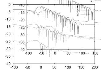
FIG. 12.:

FIG. 13.: Templates ($\ln|\Psi|$) of the axial GW (Fig. 11), polar GW (Fig. 12) and EM waves (Fig. 13), the three strongest eigenvectors (depicted as in Figs 8 – 10). The ”observer” is located at $R=100m$ and the parameter $a=2.001$. The part to the right of $x=0$ is the purely backscattered radiation.

Notice that the amplitudes of the strongest ringing mode are of the order of the largest amplitudes of remnants of the original radiation. This is particularly clearly manifested in the case of the strongest polar GW eigenvector. Observe also a strong deformation of the original signal just before $t=r^{*}(100m)$; initial waveform would be zero at $x=0$, while in Figs 10 – 13 one can see a gradual build-up of a backscattered signal. Again the effect is strongest for the polar GW (Fig. 12, the 1st eigenvector), when the backscattered part exceeds the remaining signal by a factor of 10. We would also like to direct the attention of the reader to Fig. 10. There the ringing is absent for the second and third eigenvector, but a very strong pre-tail term is observed, comparable to the remainder of the main signal.

These examples essentially confirm our conjecture that there exists a correlation between the diffusion factor and some features (strongest QNM and/or the longevity of the ringing phase) of the ringing. (The reservation ”essentially” is caused by the fact, that the ringing belonging to the second axial mode on Fig. 12 is stronger than that of the first eigenvector; but in this case the diffusion parameters differ only by the factor of 2.) An intuitive explanation with analytic flavour would be following. There is effectively $(\partial_{t}\Psi)^{2}$ contribution to the observed energy flux, if an observation point is located far away from the horizon (the asymptotic zone, where radiation is dominated by the $\Psi_{0}$-type term and $\partial_{t}\Psi\approx-\partial_{r^{*}}\Psi$). Quasinormal modes oscillate and therefore they give a more significant contribution to the total backscattered energy than, say, tail terms. Hence small $\kappa$ would be prohibitive for any ringing, while strong $\kappa$ leaves this possibility open. This reasoning suggests also that the diffused energy might well be the best measure (imperfect, admittedly) of the energy of quasinormal modes generated by moving wave pulses.

It was reported earlier (see, for instance, Sec. IX in [35]) that there exists a (sharp value of) critical width (suitably defined) of initial data corresponding to strong ringing and that both (sub- and super-) critical data generate much weaker ringing. While we observe a kind of a similar dependence, it is certainly less dramatic and no sharp indicator seems to be appropriate. Admittedly, we deal with a different situation – there is only an (initially) outgoing radiation, while in [35] there are both (initially) ingoing and outgoing components – but that probably is not relevant. More important can be a different shape of initial data – here determined by the extremization procedure of the preceding section, while in [35] assumed to be gaussian.

V Linear versus nonlinear descriptions of the post-merger evolution

A How typical are ringing modes

That is a basic tenet of the General Relativity, dictated by the beliefs in the cosmic censorship [33] and no-hair conjectures [34], that at some stage after plunge/merger a geometry generated by a pair of black holes can be represented as a single perturbed black hole. The perturbations would be represented by gravitational waves and the final black hole would be either spinning (the Kerr black hole) or nonspinning (the Schwarzschild black hole), the latter in the case of the head-on collision. The so-called close limit approximation ([36], [37], [38]) seems to assert that the linear approximation is valid since the formation of a common apparent horizon. Anninos et al.[37] give some arguments in favour of this claim that are supported (albeit with some reservations) by their analysis of the head-on collisions [39], with initial data of Misner type [40]. Gomez et al. [41] provide other supporting arguments in their discussion of fissioning white holes. An interesting new feature of a recent work by Husa et al. [42], which uses close approximation, is a weak dependence of waveforms on the collision velocity of two black holes.

If this scenario is right then the naive expectation would be that most of the radiation is concentrated in the vicinity of the horizon [43]. (This is in fact observed – see Fig. 10 in [37], which shows that initial perturbation extends to regions very close to $R=2m$.) One can split these initial data into initially ingoing and outgoing parts, according to the descriptions of Secs 2.B and 2.C. (In the example given in Fig. 10 of [37] the ingoing radiation remains forever inside the potential well [44].) The latter can be expanded in the diagonalizing basis defined in Sec. III and consisting of 250 base vectors, with the parameter $a$ (that in fact specifies this basis - see Sec. III) being very close to $2m$. But if $a\approx 2m$, then Sec. IV.A suggests that there appear a number of eigenvectors (from at least 2 for EW to at least 4-5 in the case of polar GW) with diffusion parameters being close to 1. The initial data for the linear phase are determined by the preceding nonlinear evolution; if these were purely random, then the chance of having large $\kappa$ (and strong ringing) would be of the order of 1%. Leaving aside the question whether the merger phase can be regarded as a random process, the least one can say is that the maximizing initial data of Sec. III should not be apriori excluded. Another argument is that the process of the backscatter is selective – waves longer than QNM’s are stronger backscattered. Since the present gravitational wave detectors are tuned to frequences smaller (even by one order in the case of less massive binaries of black holes [36]) than QNM’s characteristic for the most likely sources of the gravitational radiation, there are reasons to expect that the detected radiation will be strongly backscattered (even if the ringing itself would be undetectable).

B Taking of waveforms – some parameters

We pointed out in Sec. IV. B that in some examples the templates are unstable with respect to the change of the “observation” point. No significant changes in the wave profiles have been observed beyond $100m$, but the wave profiles at $R=25m$ can be profoundly different from those taken at the former point. This suggests that the determination of templates should be done at $R\gg 25m$ and that $R=100m$ might the smallest required distance of the observer. In some cases the duration of the remnants of the original signal and of the comparable in strength backscattered part exceeds $150m$ (see Fig. 12). From this one can infer that the minimal integration time must exceed at least $150m$; it happens to be the longer the closer the initial pulse is located to the horizon of a black hole. There is no numerical calculation, in the case of the full nonlinear collisions, up to our knowledge, which satisfies both requirements. For instance in [37], the observations were held at $R=25m$ through the time interval $100m$.

VI Concluding remarks

The Schwarzschild spacetime can be believed to provide a good approximation to the last phase of the collapse of two black holes – the so-called close limit ([36] – [38]) bases on this idea – provided that the collision is (almost) head-on. At this stage the spacetime can be regarded as consisting of a single black hole having a mass $m$ and some gravitational radiation that propagates on a Schwarzschlidean background. The initial data for the linear evolution of the gravitational radiation should be provided by a numerical solution of the preceding phases of the collapse. This task is at present (and presumably for some years to come) unavailable for numerical relativists. In this context the existence of universal imprints of the spacetime curvature like QNM’s could be of relevance, but only if their amplitudes are strong enough.

We invent a variational procedure that generates initial data corresponding to the strong backscatter. These initial data have some features that might look as counter-intuitive; they have an extended support and a significant fraction of the wave signal energy comes from a distant region ($R\gg 2m$). They generate strong ringing modes or (if the ringing is absent) robust terms preceding the tail. In many cases the backscattered terms and QNM’s are much stronger than the remnants of the original signal; therefore the QNM’s waveforms cannot be ruled out as objects of interest for the gravitational wave astrophysics.

Finally, it has been shown how from the linear description one can get clues as to the preparation of templates in the numerical analysis of the full nonliner problem of collapsing (head-on) black holes.

Acknowledgments. EM thanks Bernd Schmidt, Edward Seidel and Jonathan Thornburg for discussions and interesting remarks. This work has been suported in part by the KBN grant 2 PO3B 006 23. ZS thanks the Pedagogical University for the research grant.

REFERENCES

- [1] J. Hadamard Lectures on Cauchy’s problem in linear partial differential equations, Yale University Press, Yale, New Haven 1923.
- [2] B. De Witt and R. W. Brehme,Annals Phys. 9, 220(1960).
- [3] W. Kundt and E. T. Newman, J. Math. Phys. 9, 2193(1968).
- [4] R. G. McLenaghan, Proc. Camb. Phil. Soc. 65, 139(1969).
- [5] W. B. Bonnor an M. A. Rotenberg, Proc. R. Soc. A289, 2471967.
- [6] C. V. Vishveshwara, Nature 227, 936(1970).
- [7] W. H. Press, ApJ 170, L105(1971).
- [8] R. Price, Phys. Rev. D5, 2419(1972).
- [9] J. M. Bardeen and W. H. Press, J. Math. Phys. 14, 7(1973).
- [10] B. Mashhoon, Phys. Rev. D7, 2807(1973).
- [11] J. Bicak, Gen. Rel. Grav. 3, 331(1972); ibid, 12, 195(1980).
- [12] S. Chandrasekhar, The Mathematical Theory of Black Holes, Oxford: Clarendon 1983.
- [13] V. Ferrari and B. Mashhoon, Phys. Rev. Lett. 52, 1361(1984); Phys. Rev. D30, 295(1984).
- [14] E. W. Leaver, Proc. R. Soc. London, Ser. A402, 286(1986).
- [15] N. Andersson, Proc. R. Soc. London 439, 47(1992).
- [16] H. G. Nollert and B. Schmidt, Phys. Rev. D45, 2617(1992).
- [17] L. Blanchet and G. Schäfer Class. Quantum Grav. 10, 2699(1993).
- [18] E. S. C. Ching et al., Phys. Rev. Lett. 74, 2414(1995); Phys. Rev. D52, 2118(1995).
- [19] E. Malec, N. O’Murchadha and T. Chmaj, Class. Quantum Grav., 15, 1653(1998).
- [20] K. D. Kokkotas and B. Schmidt, Quasi-Normal Modes of Stars and Black Holes in Living Reviews in Relativity, published 16 Sept. 1999.
- [21] H. P. Nollert, Class. Quantum Grav. 16, R159(1999).
- [22] K. Roszkowski, Class. Quantum Grav. 18, 2305(2001).
- [23] J. Stalker, a lecture delivered during the Cargese Summer School (2002).
- [24] J. Karkowski, E. Malec and Z. Świerczyński, Acta Phys. Pol. B34, 59(2003).
- [25] F. Zerilli, Phys. Rev. Lett. 24 , 737(1970); Phys. Rev. D2, 2141(1970).
- [26] T. Regge and J. A. Wheeler, Phys. Rev. 108, 1063(1957).
- [27] J. Karkowski, E. Malec and Z. Świerczyński, Acta Phys. Pol., B32, 3593(2001).
- [28] J. Karkowski, E. Malec and Z. Świerczyński, Classical and Quantum Gravity, 19, 953(2002).
- [29] E. Malec and G. Schäfer, Phys. Rev. D64 (2001) 044012.
- [30] E. Malec, Phys. Rev. D62(2000), 084034.
- [31] The estimates are relatively sharp for the EW and axial GW [28] and [27] and exclude any significant backscatter at and , respectively. The estimates of [29] for the polar GW require some enhancement, but they are effective for .
- [32] seems to be the canonical choice for the determination of waveforms - see [37].
- [33] R. Penrose, Rivista N. Cim. 1, 252(1969).
- [34] P. Mazur, J. Phys. A15, 3173(1982).
- [35] N. Andersson, Phys. Rev. D51, 353(1994).
- [36] J. Pullin, Prog. Theor. Phys. Suppl. 136, 107(1999).
- [37] P. Anninos, R. H. Price, J. Pullin, E. Seidel and W.-M. Suen, Phys.Rev. D52,4462-4480 (1995).
- [38] R. Gleiser, G. Khanna, R. Price, J. Pullin, New Jour.Phys. 2, 3(2000).
- [39] L. Smarr, A. Ćadeź, B. De Witt and K. Eppley, Phys. Rev. D14, 2443(1976).
- [40] C. Misner, Phys. Rev. 118, 1110(1960).
- [41] R. Gomez, S. Husa, L. Lehner and J. Winicour, Phys.Rev. D66 (2002), 064019.
- [42] S. Husa, Y. Zlochower, R. Gomez and J. Winicour, Phys.Rev. D65 (2002), 084034.
- [43] This is plausible and implicitly always assumed to be true by numerical relativists but remains unproven. The main difficulty has its roots in the absence of the notion of the local energy density for free gravitational fields.
- [44] The r. h. s. of Eq. (2) becomes very small when and the ingoing part is not backscattered near the horizon.