Cauchy horizon stability in self-similar collapse: scalar radiation.

Abstract

The stability of the Cauchy horizon in spherically symmetric self-similar collapse is studied by determining the flux of scalar radiation impinging on the horizon. This flux is found to be finite.

I Introduction

Perhaps the richest source of examples of space-times admitting naked singularities is the class of spherically symmetric self-similar space-times. There is an extensive literature on the topic; the recent review of self-similarity in general relativity by Carr and Coley carr (1) provides a suitable bibliography. Of particular note in this class are the perfect fluid solutions studied by Ori and Piran OP (2), the massless scalar field solutions studied by Christodoulou christo1 (3) and by Brady brady (4) and the $SU(2)$ sigma model solutions studied by Bizon and Wasserman bizon (5). We mention these because (i) the matter model has particular interest, for either physical or mathematical reasons and (ii) these self-similar solutions are of interest in studies of critical phenomenon gundlach (6). More generally, self-similar solutions admitting naked singularities are of interest because of what they may tell us about cosmic censorship. Intriguingly, the evidence is not all in one direction. Recent work has indicated the stability of perfect fluids admitting naked singularities in the class of perfect fluid space-times harada (7), while for the case of the massless scalar field, generic spherical perturbations of self-similar initial data which correspond to naked singularities will lead to censored singularities christo2 (8). Also, within the class of self-similar spherically symmetric space-times, the sectors corresponding to censored and to naked singularities are both topologically stable nolan (9).

With these results in mind, the aim here is to begin a comprehensive study of the stability of Cauchy horizons in self-similar collapse. In the case of charged rotating black holes, the instability of the Cauchy (or inner) horizon has been firmly established (see brady2 (10) for a review). This instability is in one way easily understood; an observer crossing the inner horizon views the entire history of the external universe in a finite amount of proper time, and so time-dependent perturbations of the exterior suffer an infinite blue-shift on crossing the horizon. This instability mechanism which can be “read off” the conformal diagram, does not have a counterpart in self-similar collapse which leads to globally naked singularities (see Figures 1 and 2). At best, one can speculate that the curvature at the regular center which diverges in the limit as the scaling origin is approached makes itself felt by perturbations approaching the Cauchy horizon. This is by no means convincing, and so a rigorous analysis is required. We begin this analysis here by studying the propagation of scalar radiation in a fixed background (spherically symmetric, self-similar) space-time which admits a Cauchy horizon.

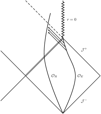
Figure 1: A portion of the conformal diagram of the maximally extended Reissner-Nordström space-time. The observer $\cal{O}_{R}$ falls through the event horizon (double line) and into the black hole. On crossing the Cauchy horizon (dashed) into a new asymptotically flat region, ${\cal{O}}_{R}$ receives in finite time all the radiation emitted by ${\cal{O}}_{E}$ during its infinite history.

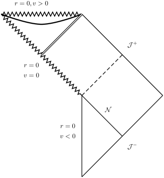
Figure 2: Conformal diagram for an example of a self-similar space-time admitting a globally naked singularity. We use the advanced Bondi co-ordinates $v$ and $r$ described in Section 2. The Cauchy horizon is shown dashed, the event horizon as a double line and the apparent horizon as a bold curve. ${\cal{N}}$ is the past null cone of the scaling origin. Other structures can arise; there may be no apparent or event horizon; the censored portion of the singularity may be null; the naked portion of the singularity may be time-like. There is evidence that the naked singularity is generically globally naked. See nolan (9) for details. In every case for which the singularity is naked, the conformal diagram fails to display an obvious mechanism by which the Cauchy horizon may be destroyed, in contrast to the case illustrated in Figure 1.

In the following section, we define the class of space-times of interest and obtain some useful relations for the metric functions thereof. We consider spherically symmetric space-times admitting a homothetic Killing vector field whose energy-momentum tensor obeys the dominant energy condition. (A complete account of energy conditions in spherical symmetry is given in the appendix.) For generality, no further restrictions are imposed at this stage, although some differentiability conditions at the past null cone of the scaling origin and at the Cauchy horizon will be imposed. Using co-ordinates adapted to the homothety and to the past null cones of the central world-line, simple conditions can be given on the metric which determine the visibility or otherwise of the singularity at the scaling origin ${\cal{O}}$. This allows a simple way of identifying both the past null cone ${\cal{N}}$ of ${\cal{O}}$ and the Cauchy horizon ${\cal{H}}$. In Section 3, we determine the behaviour of completely general time-like geodesics (i) crossing ${\cal{N}}$ and (ii) crossing the Cauchy horizon. These are used to calculate fluxes of the scalar field at the respective surfaces. The minimally coupled scalar wave equation is studied in the next section. A mode decomposition relying on the Mellin transform is used, and the asymptotic behaviour of the general solution at ${\cal{N}}$ is determined. This is used to impose the boundary condition that an arbitrary observer with unit time-like tangent $v^{a}$ measures a finite flux $\left.v^{a}\nabla_{a}\Phi\right|_{{\cal{N}}}$. We also demand that the influx at ${\cal{J}}^{-}$ be finite. The modes not ruled out by these boundary conditions are then allowed to evolve up to the Cauchy horizon and the flux $\left.v^{a}\nabla_{a}\Phi\right|_{{\cal{H}}}$ is calculated. Our principal result is that this flux is finite for all the cases we consider.

II Self-similar spherically symmetric space-times admitting a naked singularity.

We will consider the class of space-times which have the following properties. Space-time $({\cal{M}},g)$ is spherically symmetric and admits a homothetic Killing vector field. These symmetries pick out a scaling origin ${\cal{O}}$ on the central world-line $r=0$ (which we will refer to as the axis), where $r$ is the radius function of the space-time. We assume regularity of the axis to the past of ${\cal{O}}$ and of the past null cone ${\cal{N}}$ of ${\cal{O}}$. We will use advanced Bondi co-ordinates $(v,r)$ where $v$ labels the past null cones of $r=0$ and is taken to increase into the future. Translation freedom in $v$ allows us to situate the scaling origin at $(v=0,r=0)$ and identifies $v=0$ with ${\cal{N}}$. The homothetic Killing field is

$${\vec{\xi}}=v\frac{\partial}{\partial v}+r\frac{\partial}{\partial r}.$$

The line element may be written

$$ds^{2}=-2Fe^{2\psi}dv^{2}+2e^{\psi}dvdr+r^{2}d\Omega^{2},$$ (1)

where $d\Omega^{2}$ is the line element of the unit 2-sphere. The homothetic symmetry implies that $F(v,r)=F(x),\psi(v,r)=\psi(x)$ where $x=v/r$. The only co-ordinate freedom remaining in (1) is $v\to V(v)$; this is removed by taking $v$ to measure proper time along the regular center $r=0$.

We will not specify the energy-momentum tensor of $({\cal{M}},g)$, but will demand that it satisfies the dominant energy condition. A complete description of energy conditions in spherical symmetry is given in Appendix A. Of these, the following will be used. (These are equations (41), (42) and (46) respectively.)

$$x\psi^{\prime}\leq 0,$$ (2)

$$e^{\psi}(F^{\prime}+xF^{2}e^{\psi}\psi^{\prime})\leq 0,$$ (3)

$$1-2F+2x(F^{\prime}+F\psi^{\prime})\geq 0.$$ (4)

We impose the following regularity conditions at the axis. As previously mentioned, we take $v$ to be proper time along the axis for $v<0$. Noting that $x\to-\infty$ on this portion of the axis, (1) then gives

$$\lim_{x\to-\infty}2Fe^{2\psi}=1.$$ (5)

The other regularity condition that we use is that all curvature invariants are finite on $r=0,v<0$. In the present case, the (invariant) Misner-Sharp mass is given by

$$E=\frac{r}{2}(1-2F).$$

Then $E/r^{3}$ is a curvature invariant; this term has the same units as e.g. $R$ and $\Psi_{2}$. Demanding that $E/r^{3}$ be finite on the axis yields

$$\lim_{x\to-\infty}F=\frac{1}{2}.$$ (6)

Combining (5) and (6) gives these regularity conditions:

$$F(-\infty)=\frac{1}{2},\quad\psi(-\infty)=0.$$ (7)

We define the interior region ${\cal{M}}_{int}$ of space-time to be the interior of ${\cal{N}}$, i.e. the interior of the causal past of ${\cal{O}}$. The exterior region ${\cal{M}}_{ext}$ is defined to by ${\cal{M}}={\cal{M}}_{int}\cup{\cal{N}}\cup{\cal{M}}_{ext}$. (These definitions are in line with those of christo1 (3).) We assume that the metric is regular throughout ${\cal{M}}_{int}\cup{\cal{N}}$ - this set does not include ${\cal{O}}$ - by which we mean $F,\psi\in C^{2}(-\infty,0]$. As a Cauchy horizon can only form in ${\cal{M}}_{ext}$, we assume further that $F,\psi\in C^{2}(-\infty,x_{*})$ for some $x_{*}>0$. As we will see, if a Cauchy horizon develops, it must be of the form $x=x_{c}$ for some $x_{c}>0$. Our assumption is that the metric is regular at least up until the Cauchy horizon.

Since we are studying collapse, our assumptions must include some statement of regularity - in the sense of the absence of trapped surfaces - of an initial configuration. The 2-sphere $(v,r)$ is trapped if and only if

$$\chi(v,r):=g^{ab}\nabla_{a}r\nabla_{b}r<0.$$

In the present case, this is equivalent to $F<0$, and implies that the condition for an apparent horizon is $F=0$. So in order to express the notion that the matter is initially in some non-extreme state, we rule out trapped or marginally trapped surfaces in the interior region ${\cal{M}}_{int}$. We will also demand that ${\cal{N}}$ is not foliated by marginally trapped surfaces, and so we take

$$F(x)>0\quad\hbox{for all}\quad x\in(-\infty,0].$$

Next, we point out the inevitability of there being a curvature singularity at ${\cal{O}}$. Any curvature invariant which has units $L^{-2}$ is of the form $c(x)r^{-2}$. For example,

$$\frac{E}{r^{3}}=\frac{1-2F}{2r^{2}}.$$

This term diverges as we approach ${\cal{O}}$ along the null line $x=0$ unless $F(0)=\frac{1}{2}$. But subject to the assumption that $F>0$ for $x<0$, we see that the surfaces $x=x_{c}<0$ are time-like. So we may also approach ${\cal{O}}$ along $x=x_{c}<0$, and we then see that $E/r^{3}$ diverges unless $F\equiv\frac{1}{2}$ on $(-\infty,0]$. Applying the same reasoning to the invariant

$$\frac{E}{r^{3}}+\Psi_{2}+\frac{R}{12}=\frac{1}{2r^{2}}(1-2F+2x(F^{\prime}+F\Psi^{\prime})),$$

regularity at ${\cal{O}}$ would require $\Psi\equiv 0$ on $(-\infty,0]$ (we have used the boundary condition (7) here). Hence ${\cal{M}}_{int}$ is a portion of flat space-time. So avoiding the trivial case implies the existence of a curvature singularity at ${\cal{O}}$.

Let us now prove the assertion above regarding the Cauchy horizon.

Proposition 1

Let $x_{c}$ be the first positive root of $G(x):=Fe^{\psi}=\frac{1}{x}$, if such exists and $x_{c}=+\infty$ otherwise. Then there are no future pointing outgoing radial null curves emanating from ${\cal{O}}$ in the region $x\in(0,x_{c})$.

Proof The outgoing radial null curves of (1) satisfy

$$\frac{dr}{dv}=F(x)e^{\psi}(x)=G(x).$$ (8)

Let $(v_{i},r_{i})$ be a point on a solution curve $\gamma_{i}$ of (8) in the region $0<x<x_{c}$. Then $x_{i}=v_{i}/r_{i}<x_{c}$, and so $G(x_{i})<\frac{1}{x_{i}}$. If $x_{c}$ is finite, we note that $x=x_{c}$ is a solution of (8),and so by uniqueness, $\gamma_{i}$ cannot cross $x=x_{c}$ away from ${\cal{O}}$ i.e. for $v>0$. Thus

$$\left.\frac{dx}{dv}\right|_{\gamma_{i}}=\frac{1}{r}(1-xG)>0$$

for $v\in(0,v_{i}]$. Note that this inequality is immediate when $x_{c}=+\infty$. So the inequality applies generally and says that as $v\downarrow 0$, $x$ decreases and is bounded below by $0$. Hence the limit

$$x_{l}=\lim_{v\downarrow 0}\left.x(v)\right|_{\gamma_{i}}<x_{c}$$

exists and is non-negative. Thus either $r\to r_{*}>0$ as $v\downarrow 0$ - in which case the singularity is avoided - or $r\to 0$ in the limit. In this case,

$$x_{l} = \lim_{v\downarrow 0}\frac{v}{r}$$

$$= \lim_{v\downarrow 0}\frac{1}{r^{\prime}(v)}$$

$$= \lim_{v\downarrow 0}\frac{1}{G(x)}=\frac{1}{G(x_{l})},$$

where all limits are taken along $\gamma_{i}$ and l’Hopital’s rule is used in the second line. The conclusion that $x_{l}<x_{c}$ is a root of $xG=1$ contradicts minimality of $x_{c}$ and completes the proof. $\Box$

Corollary 1

If $G(x)<\frac{1}{x}$ for all $x>0$, then the singularity ${\cal{O}}$ is censored. $\Box$

Corollary 2

If $G(x)=\frac{1}{x}$ for some values of $x>0$, then $x=x_{c}$ is the Cauchy horizon ${\cal{H}}$ of the space-time, where $x_{c}$ is the smallest positive root of $xG=1$. $\Box$

These results show an advantage of describing self-similar collapse in the co-ordinates $v$ and $r$: the visibility of the singularity at ${\cal{O}}$ (and indeed the presence of an apparent horizon $F=0$) can be read-off from the metric. More accurately, the presence of a naked singularity can be determined by tracking the evolution of metric functions, and without having to integrate geodesic equations.

An apparent horizon may form either before or after the Cauchy horizon. This horizon must be space-like, and the region lying to its future is trapped:

Proposition 2

If $F(x_{a})=0$ for some $x_{a}>0$, then $x=x_{a}$ is space-like and the region $x\geq x_{a}$ is trapped or marginally trapped.

Proof Restricting to $\Sigma_{a}:\{v=x_{a}r\}$ in (1) gives

$$\left.ds^{2}\right|_{\Sigma_{a}}=2x_{a}e^{\psi(x_{a})}(1-x_{a}G(x_{a}))dr^{2}+r^{2}d\Omega^{2},$$

which has spatial signature at $G=F=0$ when $x_{a}>0$. From (3), we see that $F^{\prime}\leq 0$ at an apparent horizon. Hence $F(x)\leq 0$ for $x\geq x_{a}$. $\Box$

We conclude this section with a lemma which will play a central role in determining the stability of ${\cal{H}}$ with respect to scalar radiation.

Lemma 1

$G^{\prime}<0$ prior to the formation of a Cauchy horizon.

Proof We note first that the results of Propositions 1 and 2 show that $0<xG<1$ for $x\in(0,x_{c})$. Then (2) gives

$$xGF\psi^{\prime}=xF^{2}e^{\psi}\psi^{\prime}>F\psi^{\prime},$$

and using (3) we get

$$F^{\prime}+F\psi^{\prime}<F^{\prime}+xF^{2}e^{\psi}\psi^{\prime}\leq 0,$$

i.e. $G^{\prime}(x)<0$ for $x\in(0,x_{c})$. $\Box$

Corollary 3

$G^{\prime}(x_{c})\leq 0$. $\Box$

We note that if $G^{\prime}(x_{c})=0$, then $\left.R_{ab}k^{a}k^{b}\right|_{{\cal{H}}}=0$, where $k^{a}$ is tangent to the outgoing radial null direction. This implies that there is no ingoing radiative flux of energy-momentum crossing the Cauchy horizon. We rule out this situation as being physically unrealistic and so we will assume that $G^{\prime}(x_{c})<0$.

III Time-like geodesics crossing ${\cal{N}}$ and ${\cal{H}}$.

The stability of the Cauchy horizon will be studied from the point of view of the behaviour of the flux of scalar radiation measured by an observer crossing the horizon. This flux is ${\cal{F}}=v^{a}\nabla_{a}\Phi$, where $\Phi$ is the scalar field and $v^{a}$ is the unit tangent to an arbitrary time-like geodesic. Thus we will need to determine the behaviour of the tangent $v^{a}$ for such arbitrary geodesics at the Cauchy horizon. Since we will impose boundary conditions on $\Phi$ in terms of the fluxes at ${\cal{N}}$, we will need to do the same at this surface. The full set of equations governing time-like geodesics may be written in the form

$${\ddot{v}}-\frac{1}{r}(x(G^{\prime}+G\psi^{\prime})-\psi^{\prime}){\dot{v}}^{2}-\frac{e^{-\psi}}{r^{3}}L^{2}, = 0$$ (9)

$$-2Ge^{\psi}{\dot{v}}^{2}+2e^{\psi}{\dot{v}}{\dot{r}}+\frac{L^{2}}{r^{2}} = -1,$$ (10)

$${\dot{\Omega}} = \frac{L}{r^{2}},$$ (11)

where the overdot represents differentiation with respect to proper time $\tau$, $L$ is the conserved angular momentum and $\Omega$ is an azimuthal angular variable. (11) plays no further role below, but is given for completeness. It is convenient to rewrite (9) and (10) as a first order system. Defining $X=(r,v,u)^{T}$ where $u:={\dot{v}}$, these equations may be written as

$${\dot{X}}=H(X)=\left(\begin{array}[]{c}\frac{e^{-\psi}}{2u}(2Ge^{\psi}u^{2}-\frac{L^{2}}{r^{2}}-1)\\ u\\ \frac{1}{r}(x(G^{\prime}+G\psi^{\prime})-\psi^{\prime})u^{2}+\frac{L^{2}}{r^{3}}e^{-\psi}\end{array}\right).$$ (12)

A future-pointing time-like geodesic crossing ${\cal{N}}$ corresponds to a solution of (12) with initial values $r_{0}>0$, $v_{0}=0$, $u_{0}>0$. The assumptions of the previous section indicate that $H$ is $C^{1}$ in a neighbourhood of $(r_{0},v_{0},u_{0})\in\mathbb{R}^{3}$, and so standard theorems imply the existence of a $C^{1}$ solution for $X$ which exists for (at least) finite duration. Note that this implies that both $v$ and $r$ (via (10)) are $C^{2}$ functions of proper time $\tau$ in a neighbourhood of ${\cal{N}}$. Thus we can apply Taylor’s theorem and write def1 (11)

$$v(\tau) = u_{o}\tau+v_{2}\tau^{2}+O(\tau^{3}),$$

$$r(\tau) = r_{0}+r_{1}\tau+O(\tau^{2}),$$

where the coefficients $v_{2},r_{1}$ can be given in terms of the initial data and metric functions and we have set $\tau=0$ at ${\cal{N}}$. From this we may write down the following result which will be required below.

Proposition 3

For any future-pointing time-like geodesic crossing ${\cal{N}}$, we have

$$v \sim u_{0}\tau,\quad{\dot{v}}\sim u_{0},$$ (13)

$$x \sim \frac{u_{0}}{r_{0}}\tau,\quad{\dot{x}}\sim\frac{u_{0}}{r_{0}},$$ (14)

as $\tau\to 0$ where $\tau=0$ on the geodesic at ${\cal{N}}$. $\Box$

Obtaining equivalent results at the Cauchy horizon is more difficult, as this corresponds to a singular point of the geodesic equations. Two things must be established: the existence of time-like geodesics crossing the horizon and the limiting values of the components of the tangent vector at the horizon. The proof below requires an assumption on the level of differentiability at the horizon which it would be desirable to remove.

Proposition 4

Suppose that $G$ and $\psi$ are differentiable at $x=x_{c}$. Then all radial time-like geodesics whose initial points are sufficiently close to the Cauchy horizon will cross the horizon in finite time. For any time-like geodesic crossing the horizon, the components of the tangent $\dot{x}$ and $\dot{v}$ have finite non-zero values at the horizon which, denoting them by $\dot{x}_{c}$ and $\dot{v}_{c}$ respectively, satisfy the relation

$$\dot{v}_{c}=\frac{1}{2}\frac{x_{c}^{2}}{v_{c}\dot{x}_{c}}e^{-\psi_{c}},$$ (15)

where the subscript refers to the value of a quantity at $x=x_{c}$.

Proof (i) First, we establish a first order non-autonomous system for the geodesics. If $\xi^{a}$ is the homothetic Killing vector field and $u^{a}$ is tangent to a time-like geodesic, then

$$\frac{d}{d\tau}(\xi_{a}u^{a})=-1,$$

where $\tau$ is proper time along the geodesic (see e.g. Appendix C of wald (12)). Integrating yields

$$g_{ab}\xi^{a}u^{b}=2\frac{v}{x}e^{\psi}(1-xG){\dot{v}}-\frac{v^{2}}{x^{2}}e^{\psi}\dot{x}=k-\tau,$$

for some $k$ which is constant along the geodesic. Combining with

$$\frac{2}{x}e^{\psi}(1-xG){\dot{v}}^{2}-\frac{2}{x^{2}}e^{\psi}v\dot{v}\dot{x}=-(1+\frac{L^{2}}{r^{2}})$$ (16)

(which is (10) written in terms of $v$ and $x$) we obtain the first order system

$${\dot{x}} = \pm\frac{x^{2}}{v^{2}}e^{-\psi}Y^{1/2},$$ (17)

$${\dot{v}} = \frac{1}{2}\frac{x}{v}e^{-\psi}(1-xG)^{-1}(-(\tau-k)\pm Y^{1/2}),$$ (18)

where

$$Y=(\tau-k)^{2}+2\frac{v^{2}}{x}(1-xG)e^{\psi}(1+\frac{L^{2}}{r^{2}}).$$

We choose the upper sign, which corresponds to future-pointing geodesics.

(ii) For radial $(L=0)$ time-like geodesics, (9) becomes

$${\ddot{v}}=(x^{2}G^{\prime}+x\psi^{\prime}(xG-1))\frac{{\dot{v}}^{2}}{v}.$$

Since $G^{\prime}(x_{c})<0$, the coefficient on the right hand side is negative for values of $x<x_{c}$ sufficiently close to $x_{c}$. Hence a geodesic with initial value $x_{0}=x(\tau_{0})$ sufficiently close to $x_{c}$ in this sense satisfies ${\ddot{v}}<0$ for $\tau\geq\tau_{0}$, and so $v$ cannot diverge to infinity in finite time.

(iii) Next, we establish that if $v\to\infty$ as $\tau\to\infty$ along a geodesic which does not cross the Cauchy horizon, then $x\to x_{c}$ as $\tau\to\infty$. From (16), we can write

$$\frac{\dot{v}}{v}<\frac{\dot{x}}{x(1-xG)}.$$

Integrating both sides yields and taking $v=v_{0}$ at some $0<x_{0}<x_{c}$, we get

$$v<v_{0}\exp\left(\int_{x_{0}}^{x}\frac{dy}{y(1-yG)}\right)$$

for $x_{0}<x$. Thus if $v$ diverges to $+\infty$, then so too must the integral. This can only occur if the integrand diverges, i.e. if $x\to x_{c}$. Now we show that provided a geodesic has initial point sufficiently close to $x=x_{c}$, it cannot behave in this way.

(iv) Consider a radial time-like geodesic for which $v\to\infty$ and $x\to x_{c}$ as $\tau\to\infty$. We have from (9)

$$\frac{v\ddot{v}}{\dot{v}^{2}}\to x_{c}^{2}G^{\prime}(x_{c})=-k^{2}<0$$

as $\tau\to\infty$. Integrating and reusing this relation yields the asymptotic relations

$$\dot{v} \sim c_{1}v^{-k^{2}},$$ (19)

$$\ddot{v} \sim -k^{2}c_{1}v^{-2k^{2}-1}$$ (20)

as $\tau\to\infty$ for some $c_{1}>0$. Using these and (16) we obtain

$$\dot{x} \sim c_{2}v^{k^{2}-1}$$ (21)

as $\tau\to\infty$ for some $c_{2}>0$. We must have $\dot{x}\to 0$ as $\tau\to\infty$, for otherwise $\dot{x}$ is positive and bounded away from zero for an infinite amount of time and so $x$ reaches $x_{c}$ in finite time. Our present assumption is that this does not happen, so we must have $k^{2}<1$.

The geodesic equations yield

$$2A\ddot{v}+vB\ddot{x}+2A^{\prime}\dot{x}\dot{v}+vB^{\prime}\dot{x}^{2}=0,$$ (22)

where

$$A(x)=\frac{2}{x}e^{\psi}(1-xG),\quad B=-\frac{2}{x^{2}}e^{\psi}.$$

Using the assumption that these terms are differentiable at the Cauchy horizon, we have from (19)-(21), def1 (11)

$$2A\ddot{v} \sim -2Ak^{2}c_{1}^{2}v^{-2k^{2}-1}=o(v^{-2k^{2}-1}),$$

$$2A^{\prime}\dot{x}\dot{v} \sim 2A^{\prime}c_{1}c_{2}v^{-1}=O(v^{-1}),$$

$$vB^{\prime}\dot{x}^{2} \sim B^{\prime}v^{2k^{2}-1}.$$

Comparing these with (22), we see that we must have

$$\lim_{v\to\infty}v\ddot{x}=-\lim_{v\to\infty}v\frac{B^{\prime}}{B}\dot{x}^{2}.$$

We have

$$\frac{B^{\prime}}{B}=-2x^{-1}+\psi^{\prime}.$$

Using the energy condition (2), we see that this term is strictly negative at the Cauchy horizon, and so this implies that $\ddot{x}$ is positive for sufficiently large values of $\tau$. However this contradicts the fact that $\dot{x}(\tau)>0$ with $\dot{x}\to 0$ as $\tau\to 0$. Hence the geodesic cannot extend to arbitrarily large values of $v$ without first crossing the Cauchy horizon.

(v) To conclude, it has been established that (at least some) radial geodesics cross the horizon in finite time and so with a finite value $v_{c}$ of $v$. For any such geodesic, including non-radials, we can read off from (17) the non-zero and finite limiting value of $\dot{x}$ and from (16) we obtain (15). ${\Box}$

IV The scalar field on the Cauchy horizon.

Now we are in a position to examine the stability of the Cauchy horizon by measuring the flux of the scalar field in different regions of the space-time.
In order to measure the flux $\mathcal{F}=v^{a}\nabla_{a}\Phi$ we need first the solution of the scalar wave equation,

$$\Box\Phi=(-g)^{-\frac{1}{2}}\partial_{a}\left[(-g)^{\frac{1}{2}}g^{ab}\partial_{b}\Phi\right]=0.$$

We exploit the spherical symmetry of the space time and split the scalar field,

$$\Phi(v,x,\theta,\phi)=T(v,x)A(\theta,\phi),$$

where we use the advanced null coordinate $v$, the homothetic coordinate $x$, and the standard angular coordinates $\theta,\phi$. Then the line element in these co-ordinates reads

$$ds^{2}=2e^{\psi}\left(\frac{1}{x}-G\right)dv^{2}-\frac{2e^{\psi}v}{x^{2}}dvdx+\frac{v^{2}}{x^{2}}d\Omega^{2}.$$

By using separation of variables we arrive at a p.d.e. in $v,x$

$$2x^{2}\left(\frac{1}{x}-G\right)T,_{xx}+2vT,_{xv}-2x^{2}G^{\prime}T,_{x}$$

$$-2vT,_{v}-\rho e^{\psi}T=0$$ (23)

where $\rho=l(l+1)$ is the separation constant, $l=0,1,2\ldots$ is the multipole mode number, and ^′ denotes differentiation w.r.t.$\>x$. The complementary p.d.e. in $\theta,\phi$ reduces to a form of Legendre’s equation and is solved by the spherical harmonic functions, $P^{m}_{l}(\theta,\phi)$.
We can perform a Mellin transformation on the field, defined by

$$M\{T\}(x,n)=H_{n}(x)=\int_{0}^{\infty}T(v,x)v^{n-1}dv$$

which amounts to replacing $T(v,x)$ with $v^{n}H_{n}(x)$, where $n$ is an as yet unconstrained complex parameter. Equation (23) thus reduces to an o.d.e. in $H(x)$,

$$2x^{2}\left(\frac{1}{x}-G\right)H^{\prime\prime}+(2n-2x^{2}G^{\prime})H^{\prime}$$

$$-\left(\frac{2n}{x}+\rho e^{\psi}\right)H=0$$ (24)

where we have suppressed the subscript $n$. Performing the inverse Mellin transform on the solution of this o.d.e. over a contour in the viable range of $n$ will return the solution to (23).
This o.d.e. has a number of singular points, namely $x=0$ and the roots of $xG=1$, the lowest of which we have defined to be $x_{c}$. The canonical form of a second order linear o.d.e. in a neighborhood of $x=x_{0}$ is

$$(x-x_{0})^{2}H^{\prime\prime}+(x-x_{0})q(x)H^{\prime}+p(x)H=0,$$

and when we write equation (24) in its canonical form in the neighborhood of $x=0$, we find

$$q(x)=\frac{n-x^{2}G^{\prime}}{1-xG},\qquad p(x)=-\frac{2n+\rho e^{\psi}x}{2(1-xG)}.$$

Since $q(x)$ and $p(x)$ are both $C^{1}$ in a neighborhood of $x=0$ we can use the method of Frobenius to solve (24) on $\mathcal{N}$ foot (13) (see e.g. Chapter 3 of BendOr (14)). The indicial exponents are $1,-n$.
As it stands we cannot make any assumptions about $n$, however later analysis shows if $-\textrm{Re}(n)\geq 1$ the flux of the scalar field will be always infinite on $\mathcal{N}$, thus we only consider $-\textrm{Re}(n)<1$.
It is possible for $1$ and $-n$ to differ by an integer and so the method of Frobenius yields the following expression for the solution to (24) in a neighborhood of $x=0$,

$$H(x)=c_{1}\sum_{m=0}^{\infty}a_{m}x^{m+1}$$

$$+c_{2}\left\{k\ln x\sum_{m=0}^{\infty}a_{m}x^{m_{+}1}+\sum_{m=0}^{\infty}b_{m}x^{m-n}\right\}.$$ (25)

In this expression, $c_{1}$ and $c_{2}$ are arbitrary constants, $a_{0}=b_{0}=1$ with $k=0$ if $1$ and $-n$ do not differ by an integer, $a_{0}=1,b_{0}=0$ with $k=1$ if $1$ and $-n$ are equal, and $a_{0}=b_{0}=1$ with $k\neq 0$ if $1+n=m$ for some positive integer $m$.
After some rearranging and some cancellations, the expression for the flux on $\mathcal{N}$ is

$$\mathcal{F}_{1}(v,r)=\dot{v}\sum_{m=0}^{\infty}a_{m}(m+n+1)\frac{v^{n+m}}{r^{m+1}}$$

$$-\dot{r}\sum_{m=0}^{\infty}a_{m}(m+1)\frac{v^{m+n+1}}{r^{m+2}}$$ (26)

$$\mathcal{F}_{2}(v,r)=\dot{v}\sum_{m=0}^{\infty}b_{m+1}(m+1)\frac{v^{m}}{r^{m-n+1}}$$

$$-\dot{r}\sum_{m=0}^{\infty}b_{m}(m-n)\frac{v^{m}}{r^{m-n+1}}$$

$$-\dot{r}k\sum_{m=0}^{\infty}\left[1+(m+1)\ln\left(\frac{v}{r}\right)\right]a_{m}\frac{v^{n+m+1}}{r^{m+2}}$$

$$+\dot{v}k\sum_{m=0}^{\infty}\left[1+(m+n+1)\ln\left(\frac{v}{r}\right)\right]a_{m}\frac{v^{m+n}}{r^{m+1}}.$$ (27)

where the $1$ subscript denotes the $c_{1}$ part, and likewise the $2$ subscript.
The components of the velocity have been shown to be finite on $\mathcal{N}$ in Proposition 3, and we see that for the flux to have a finite measure on $\mathcal{N}$, that is when $v=0$, we require

$$\textrm{Re}(n)>0.$$

Under this condition we let the scalar field evolve towards $\mathcal{H}$, and examine its flux there.
Note: A scalar field coming from past null infinity will have a finite flux thereon if $\textrm{Re}(n)\leq 1$. While this physically desirable condition should be imposed, it does not play any role in later analysis.

When we write (24) in its canonical form around $x=x_{c}$, we find the coefficients are

$$q(x)=\left(\frac{x-x_{c}}{x}\right)\left(\frac{n-x^{2}G^{\prime}}{1-xG}\right)$$

$$p(x)=\left(\frac{x-x_{c}}{x}\right)^{2}\left(\frac{n+\frac{\rho e^{\psi}x}{2}}{1-xG}\right).$$

Now we reach an important distinction, whether $G(x)$ has a unique lowest root or multiple lowest roots. We distinguish the two cases so:

Lemma 2

When $xG=1$ has a unique lowest root,

$$x_{c}^{2}G^{\prime}(x_{c})+1>0.$$

When $xG=1$ has a multiple lowest root,

$$x_{c}^{2}G^{\prime}(x_{c})+1=0.$$

$\Box$

The two cases will lead to very different analyses, thus we treat them separately.

(i) The first case leads to $q(x),p(x)$ being $C^{1}$ on $x=x_{c}$, thus $x_{c}$ is a regular singular point and hence we can use the method of Frobenius. The indicial exponents are $0,1-q_{0}$ where

$$q_{0}=\frac{x_{c}^{2}G^{\prime}(x_{c})-n}{x_{c}^{2}G^{\prime}(x_{c})+1}.$$

Since $n>0$, Lemma $1$ and $2$ tell us $q_{0}<0$, hence $1-q_{0}>0$, which gives us

$$H(x)=C_{1}\sum_{m=0}^{\infty}A_{m}\zeta^{m+1-q_{0}}$$

$$+C_{2}\left\{k\ln\zeta\sum_{m=0}^{\infty}A_{m}\zeta^{m+1-q_{0}}+\sum_{m=0}^{\infty}B_{m}\zeta^{m}\right\}$$ (28)

where $\zeta=x-x_{c}$, and the coefficients have the same structure as (25). From this we calculate the flux,

$$\mathcal{F}_{1}=\dot{x}v^{n}C_{1}\sum_{m=0}^{\infty}(m+1-q_{0})A_{m}\zeta^{m-q_{0}}$$

$$+\dot{v}nv^{n-1}C_{1}\sum_{m=0}^{\infty}A_{m}\zeta^{m+1-q_{0}}$$ (29)

$$\mathcal{F}_{2}=\dot{x}v^{n}C_{2}\Bigg{[}k\sum_{m=0}^{\infty}A_{m}\left[\ln\zeta(m+1-q_{0})+1\right]\zeta^{m-q_{0}}$$

$$+\sum_{m=0}^{\infty}B_{m}m\zeta^{m-1}\Bigg{]}$$

$$+\dot{v}nv^{n-1}C_{2}\left[\sum_{m=0}^{\infty}B_{m}\zeta^{m}+k\ln\zeta\sum_{m=0}^{\infty}A_{m}\zeta^{m+1-q_{0}}\right].$$ (30)

Using the finiteness of $\dot{v},\dot{x}$ given in Proposition 4, we see that if $q_{0}<0$, that is if $n>0$, this expression is finite on $\mathcal{H}$, i.e. when $x-x_{c}=\zeta=0$.
Thus in the case of $xG=1$ having a unique lowest root, a scalar field measuring a finite flux entering the region will measure a finite flux on the Cauchy horizon.

(ii) If $x_{c}^{2}G^{\prime}(x_{c})+1=0$, $x_{c}$ is an irregular singular point of (24). Note that this is a special case which one would expect to correspond to a set of measure zero in the class of space-times under consideration. We label $\eta=x_{c}-x$ and examine solutions to the o.d.e. in the asymptotic limit $\eta\downarrow 0$ (see e.g. Chapter 3 of BendOr (14)).
We assume the solution to (24) can be written in the form

$$H(\eta)=e^{S(\eta)},$$

reducing (24) to an o.d.e. in $S$. Now we assume the common property near irregular singular points,

$$\ddot{S}=o(\dot{S}^{2}),\qquad\eta\downarrow 0$$

where the overdot denotes differentiation with respect to $\eta$. (24) becomes a quadratic in $\dot{S}$,

$$\dot{S}^{2}\left\{(x_{c}-\eta)-(x_{c}-\eta)^{2}G\right\}-\left(n+(x_{c}-\eta)^{2}\dot{G}\right)\dot{S}$$

$$\sim\frac{n}{x_{c}-\eta}+\frac{\rho e^{\psi}}{2},\qquad\eta\downarrow 0$$ (31)

If we consider $xG=1$ to have a lowest root of multiplicity $k$, then we can write its Taylor series around $\eta=0$ as

$$1-(x_{c}-\eta)G(\eta)=P(\eta)=\eta^{k}\frac{P^{(k)}(0)}{k!}+O(\eta^{k+1})$$

This means if the lowest root is of multiplicity $k$, we need the metric functions to be $C^{k}$. This is not too much of a restriction however, since the class of functions with roots of multiplicity $k$ becomes very small as $k$ increases, meaning we are dealing with a very special case in this analysis.
We can make the approximation

$$n+(x_{c}-\eta)^{2}\dot{G} \sim n+1,\qquad\eta\downarrow 0,$$

and since we assume the metric coefficients are at least $C^{2}$, we can approximate $e^{\psi}$ by the first term in its expansion, $c_{0}$, in the limit $\eta\downarrow 0$. Thus we arrive at a quadratic in $S$,

$$\eta^{k}(\dot{S})^{2}-\alpha\dot{S}\sim\beta,\qquad\eta\downarrow 0,\qquad\qquad$$ (32)

$$\alpha=\frac{k!(n+1)}{x_{c}P^{(k)}(0)},\quad\beta=\frac{k!}{x_{c}P^{(k)}(0)}\left(\frac{n}{x_{c}}+\frac{\rho c_{0}}{2}\right)$$

where $\alpha,\beta>0$ (if $Re(n)>0$) and constant in the limit $\eta\downarrow 0$, and $k>1$. This quadratic has two solutions corresponding to two linearly independent solutions of (24), which are

$$S_{1} \sim -\frac{\alpha}{(k-1)}\eta^{1-k}+O(\eta)$$

$$S_{2} \sim -\frac{\beta}{\alpha}\eta+\frac{\beta^{2}}{\alpha^{3}}\frac{\eta^{k+1}}{(k+1)}+O(\eta^{2k+1}),\qquad\eta\downarrow 0.$$

At this point we verify our earlier assumption, namely

$$\ddot{S}=o(\dot{S}^{2}),\qquad\eta\downarrow 0.$$

Thus we have constructed two solutions to (24),

$$H_{1}(\eta) = \eta^{k}\exp\left\{-\frac{\alpha}{(k-1)}\eta^{1-k}+O(\eta)\right\}$$ (33)

$$H_{2}(\eta) = \exp\{O(\eta)\}$$ (34)

Both of these functions and their derivatives are finite in the limit $\eta\downarrow 0$, $x\rightarrow x_{c}$ if $Re(n)>0$, and thus the resulting expressions for the flux are finite, where again we use Proposition 4.
We summarize thus:

Proposition 5

Let space-time ($\mathcal{M}$,g) satisfy the requirements of Section II and admit a Cauchy horizon $x=x_{c}$. Assume also that $g_{ab}\in C^{2}$ at $x=x_{c}$. Then a scalar field which has a finite flux on $\mathcal{N}$, the past null cone of $\mathcal{O}$, will also have a finite flux on the Cauchy horizon, $\mathcal{H}$.

V Conclusions

We have shown that the Cauchy horizon formed by collapse in a self similar, spherically symmetric space-time is stable with respect to scalar radiation. This space-time is very general, the only other constraints being that the field satisfies the dominant energy condition, and, other than the special case discussed in Section IV(ii), we require the metric functions to be $C^{2}$ on ${\cal{N}}$ and ${\cal{H}}$. These differentiability conditions are stronger than one would like to assume (cf. the $C^{0}$ Cauchy horizons appearing in the collapse of wave maps bizon (5)), but are as low as one can go without having to resort to a generalised solution concept for the wave equation.
The next step is to examine whether linear perturbations of the metric functions will lead to an unstable Cauchy horizon, as is seen, for example, in the Reissner-Nordström solution. Such an examination would be more significant in considering cosmic censorship. Is it difficult to anticipate the general outcome of such an examination. One expects to observe instability for the case of a massless scalar field christo2 (8), but stability for (some sectors of) perfect fluid collapse harada (7). The present results and the Cauchy horizon stability conjecture would lead one to expect stability in general debbie (15).

Appendix A Energy conditions in spherical symmetry

A.1 Spherical symmetry

We write the line element in double null coordinates;

$$ds^{2}=-2e^{-2f}dudv+r^{2}d\Omega^{2},$$

where $f=f(u,v)$, $r=r(u,v)$ and $d\Omega^{2}$ is the line element on the unit 2-sphere. The non-vanishing Ricci tensor terms are

$$R_{uu} = -2r^{-1}(r_{uu}+2r_{u}f_{u}),$$

$$R_{vv} = -2r^{-1}(r_{vv}+2r_{v}f_{v}),$$

$$R_{uv} = -2r^{-1}(r_{uv}-rf_{uv}),$$

$$R_{\theta\theta} = \csc^{2}\theta R_{\phi\phi}=2\frac{E}{r}+2e^{2f}rr_{uv},$$

where $E$ is the Misner-Sharp mass,

$$E=\frac{r}{2}(1+2e^{2f}r_{u}r_{v}).$$

Subscripts on $f,r$ denote partial derivatives. The only non-vanishing Weyl tensor term is

$$\Psi_{2} = -\frac{1}{3}\frac{E}{r^{3}}+\frac{1}{3}e^{2f}(f_{uv}+r^{-1}r_{uv})$$

$$= -\frac{E}{r^{3}}-\frac{1}{12}g^{AB}R_{AB}+\frac{R_{\theta\theta}}{3r^{2}},$$

where $x^{A}$ are co-ordinates in the Lorentzian 2-space.

A.2 The strong energy condition

Our aim is to write down a set of conditions on the curvature terms listed above which are equivalent to the strong energy condition:

$$R_{ab}v^{a}v^{b}\geq 0$$

for all (future-pointing) causal vectors ${\vec{v}}$.

A.2.1 Null vectors

The radial null directions are $\delta^{a}_{u},\delta^{a}_{v}$. These give

$$R_{uu}\geq 0,\qquad R_{vv}\geq 0.$$

At any point, the general non-radial null direction may be written as

$$v^{a}=\alpha\delta^{a}_{u}+\beta\delta^{a}_{v}+\gamma\delta^{a}_{\phi}.$$ (35)

The null condition is

$$\alpha\beta=2r^{2}e^{2f}\gamma^{2}.$$

We find

$$R_{ab}v^{a}v^{b}=\alpha^{2}R_{uu}+\beta^{2}R_{vv}+2\alpha\beta(2f_{uv}+2\frac{E}{r^{3}}e^{-2f}).$$

This is non-negative for all non-radial null vectors if and only if it is non-negative for all values of $\alpha,\beta$ with $\alpha\beta>0$. In turn, this is true if

$$\min_{\mu>0}Q(\mu)\geq 0,$$

where $\mu=\alpha/\beta>0$ and

$$Q(\mu)=\mu^{2}R_{uu}+2\mu(2f_{uv}+2\frac{E}{r^{3}}e^{-2f})+R_{vv}.$$

If $R_{uu}=R_{vv}=0$, this is simply

$$f_{uv}+\frac{E}{r^{3}}e^{-2f}\geq 0.$$

If $R_{uu}=0$ and $R_{vv}\neq 0$, the condition is equivalent to

$$2\mu(2f_{uv}+2\frac{E}{r^{3}}e^{-2f})+R_{vv}\geq 0$$

for all $\mu>0$. This is satisfied if $f_{uv}+\frac{E}{r^{3}}e^{-2f}\geq 0$. If $f_{uv}+\frac{E}{r^{3}}e^{-2f}<0$, then the condition will be violated for sufficiently large values of $\mu$ (which can always be chosen). The same holds for $R_{uu}\neq 0,R_{vv}=0$. Thus if $R_{uu}R_{vv}=0$, the strong energy condition holds for null directions if and only if

$$f_{uv}+\frac{E}{r^{3}}e^{-2f}\geq 0.$$

So now assume that $R_{uu}>0$, $R_{vv}>0$. The quadratic $Q(\mu)$ has a global minimum at

$$\mu_{*}=-2R_{uu}^{-1}(f_{uv}+\frac{E}{r^{3}}e^{-2f}),$$

while $Q(0)=R_{vv}>0$. Thus $Q(\mu)>0$ for $\mu>0$ if and only if either $\mu_{*}\leq 0$ or $\mu_{*}>0$ and $Q(\mu_{*})\geq 0$.

$\mu_{*}\leq 0$ if and only if $f_{uv}+\frac{E}{r^{3}}e^{-2f}\geq 0$.

$\mu_{*}>0$ if and only if $f_{uv}+\frac{E}{r^{3}}e^{-2f}<0$. In this case,

$$Q(\mu_{*}) = -4R_{uu}^{-1}(f_{uv}+\frac{E}{r^{3}}e^{-2f})^{2}+R_{vv}\geq 0$$

$$\Leftrightarrow |f_{uv}+\frac{E}{r^{3}}e^{-2f}|\leq\frac{1}{2}(R_{uu}R_{vv})^{1/2}$$

$$\Leftrightarrow f_{uv}+\frac{E}{r^{3}}e^{-2f}\geq-\frac{1}{2}(R_{uu}R_{vv})^{1/2}.$$

Combining these results, we can say:

$R_{ab}v^{a}v^{b}\geq 0$ for all null $v^{a}$ if and only if

$$R_{uu} \geq 0$$ (36)

$$R_{vv} \geq 0$$ (37)

$$\frac{1}{2}(R_{uu}R_{vv})^{1/2}+f_{uv}+\frac{E}{r^{3}}e^{-2f} \geq 0.$$ (38)

A.2.2 Time-like vectors

Again we write

$$v^{a}=\alpha\delta^{a}_{u}+\beta\delta^{a}_{v}+\gamma\delta^{a}_{\phi},$$

and we can use the time-like condition $g_{ab}v^{a}v^{b}=-1$, so that

$$\gamma^{2}=r^{-2}(2e^{-2f}\alpha\beta-1)\geq 0.$$

So in this case we are minimizing over the set $\alpha\beta\geq\frac{1}{2}e^{2f}$. we do this by minimizing over the hyperbola $\alpha\beta=c$ and then minimizing over all hyperbolas $c\geq\frac{1}{2}e^{2f}$. This yields the conditions above and the extra condition

$$\frac{1}{2}(R_{uu}R_{vv})^{1/2}+f_{uv}-r^{-1}r_{uv}\geq 0.$$ (39)

A.3 The weak energy condition

The weak energy condition $T_{ab}v^{a}v^{b}\geq 0$ for all causal $v^{a}$ can be written, using Einstein’s equation, as $R_{ab}v^{a}v^{b}\geq\epsilon R/2$, where $\epsilon=g_{ab}v^{a}v^{b}$. ($R=$ Ricci scalar.) Thus the only extra work to do is for time-like vectors. The algebra involved in the previous section only needs minute changes, and we can show that the weak energy condition is equivalent to (36) - (38) and

$$\frac{1}{2}(R_{uu}R_{vv})^{1/2}+r^{-1}r_{uv}+\frac{E}{r^{3}}e^{-2f}\geq 0.$$ (40)

A.4 The dominant energy condition

This states that for every future-pointing timelike $v^{a}$, the vector $-T^{ab}v_{b}$ is non-spacelike and future-pointing, and $T_{ab}v^{a}v^{b}\geq 0$. Using the usual general form for $v^{a}$, we again have quadratic inequalities for the parameters $\alpha$ and $\beta$ which can be treated in the usual way. (The non-spacelike condition is $g_{ac}T^{ab}T^{cd}v_{b}v_{d}\leq 0$; the left hand side is homogeneous of degree 2 in $(\alpha,\beta)$ and so quadratic in $\mu$.) The future-pointing condition is simple to examine by assuming that $u,v$ increase into the future. The resulting inequalities are

$$R_{uu} \geq 0,$$

$$R_{vv} \geq 0,$$

$$\frac{E}{r^{3}}e^{-2f}+r^{-1}r_{uv} \geq 0,$$

$$\frac{1}{2}(R_{uu}R_{vv})^{1/2}+\frac{E}{r^{3}}e^{-2f}+r^{-1}r_{uv} \geq |f_{uv}-r^{-1}r_{uv}|.$$

Using the first three of these, we see that the left hand side of the fourth is non-negative, and so the fourth is equivalent to the two inequalities

$$\frac{1}{2}(R_{uu}R_{vv})^{1/2}+\frac{E}{r^{3}}e^{-2f}+2r^{-1}r_{uv}-f_{uv} \geq 0,$$

$$\frac{1}{2}(R_{uu}R_{vv})^{1/2}+\frac{E}{r^{3}}e^{-2f}+f_{uv} \geq 0.$$

Note how (as expected) some of these are the same as some of the strong and weak energy conditions.

A.5 Summary: covariant form of the energy conditions

The energy conditions are given here in terms that use $r_{uv}$ and $f_{uv}$. A more transparently covariant form is obtained by using $R$ and $\Psi_{2}$ instead of these two. Then the results are as follows (we note that the signs of $R_{uu}$, $R_{vv}$ and the term $e^{4f}R_{uu}R_{vv}$ are invariants - the last of these is defined in terms of contractions of Ricci with the two invariantly defined radial null directions):

The strong energy condition is equivalent to

$$R_{uu} \geq 0,$$ (41)

$$R_{vv} \geq 0,$$ (42)

$$\frac{1}{2}e^{2f}|R_{uu}R_{vv}|^{1/2}+2\frac{E}{r^{3}}+2\Psi_{2}-\frac{R}{12} \geq 0,$$ (43)

$$\frac{1}{2}e^{2f}|R_{uu}R_{vv}|^{1/2}+\frac{E}{r^{3}}+\Psi_{2}-\frac{R}{6} \geq 0.$$ (44)

The weak energy condition is equivalent to (41), (42), (43) and

$$\frac{1}{2}e^{2f}|R_{uu}R_{vv}|^{1/2}+\frac{E}{r^{3}}+\Psi_{2}+\frac{R}{12} \geq 0.$$ (45)

The dominant energy condition is equivalent to (41), (42), (43) and

$$\frac{E}{r^{3}}+\Psi_{2}+\frac{R}{12} \geq 0,$$ (46)

$$\frac{1}{2}e^{2f}|R_{uu}R_{vv}|^{1/2}+\frac{R}{4} \geq 0.$$ (47)

References

• (1) Carr B J and Coley A A Class. Quantum Grav. 16 R31 (1999).
• (2) Ori A and Piran T Phys. Rev. D42 1068 (1990).
• (3) Christodoulou D Ann. Math. 140 607 (1994).
• (4) Brady P R Phys. Rev. D51 4168 (1995).
• (5) Bizon P and Wasserman A Class. Quantum Grav. 19 3309 (2002).
• (6) Gundlach, C Living Rev. Rel. 2 4 (1999).
• (7) Harada T Phys. Rev. D63 084022; Class. Quantum Grav. 18 4549 (2001).
• (8) Christodoulou D Ann. Math. 149 183 (1999).
• (9) Nolan B C Class. Quantum Grav. 18 1651 (2001).
• (10) Brady P R Prog. Theor. Phys. Suppl. 136 29 (1999).
• (11) We use the following standard notation for asymptotic relations: $f(x)=O(g(x))$ as $x\to x_{0}$ iff $\exists$ constant $k$ s.t. $|f(x)|\leq k|g(x)|,\quad x\rightarrow x_{0}$. $f(x)=o(g(x))$ as $x\to x_{0}$ iff for any $\epsilon>0,|f(x)|\leq\epsilon|g(x)|,\quad x\rightarrow x_{0}$. We define $\sim$ as $f(x)\sim g(x)$ as $x\to x_{0}$ iff $f(x)-g(x)=o(g(x))$ as $x\to x_{0}$.
• (12) Wald R M General Relativity (Univ. Chicago Press, Chicago, 1984).
• (13) To use the method of Frobenius the coefficients $q(x),p(x)$ should be analytic at $x=0$. However, to obtain the required information about $H$ it is sufficient to use a finite expansion with appropriate remainder terms, i.e.Β with $q,p\in C^{1}$ at $x=0$. Thus we only require the metric coefficients to be $C^{2}$ at $x=0$, and similarly at $x=x_{c}$. We assume this henceforth.
• (14) Bender C M and Orszag S A Asymptotic Methods and Perturbation Theory (Springer-Verlag, New York, 1999).
• (15) Konkowski D A and Helliwell T M Phys. Rev. D54 7898 (1996).