Particle creation in a tunneling universe

Abstract

An expanding closed universe filled with radiation can either recollapse or tunnel to the regime of unbounded expansion, if the cosmological constant is nonzero. We re-examine the question of particle creation during tunneling, with the purpose of resolving a long-standing controversy. Using a perturbative superspace model with a conformally coupled massless scalar field, which is known to give no particle production, we explicitly show that the breakdown of the semiclassical approximation and the “catastrophic particle production” claimed earlier in the literature are due to an inappropriate choice of the initial quantum state prior to the tunneling.

I Introduction

The tunneling approach to quantum cosmology proposes to view the creation of the Universe as a quantum tunneling event AV86 ; R84 ; ZelStar . A semiclassical picture based on the Wheeler-DeWitt equation describes tunneling from a state of vanishing size (“tunneling from nothing”) to a closed inflating universe. Alternative proposals have been put forward by Hartle and Hawking HH and Linde Linde84 . For a recent critical review see, e.g., AV02 . In the present paper, we shall focus on the tunneling picture.

The process of tunneling from nothing can be thought of as a limit of tunneling from a closed recollapsing universe of very small but nonzero size (“tunneling from something”). Consider a closed FRW universe filled with a vacuum of constant energy density and some matter or radiation. Classically, such a universe has two possible types of evolution. It can expand to a maximum radius and recollapse, or it can contract from an infinite size, bounce at a minimum radius and then reexpand. But in quantum cosmology there is yet another possibility. Instead of recollapsing, the universe can tunnel through a potential barrier to the regime of unbounded expansion. The semiclassical tunneling probability does not vanish in the limit when the maximum size of the initial universe shrinks to zero. The corresponding wave function describes quantum nucleation of an inflating universe from nothing.

The question of the particle content in the universe created by quantum tunneling has been studied in the literature by including the inhomogeneous modes of quantum fields in the wave function. Conflicting claims of excessive particle production during tunneling R84 ; LRR02 , on the one hand, and of essentially no particle content in the inflating universe V88 ; VV88 ; GV97 , on the other hand, have been advanced. In this paper we intend to resolve this controversy and explain the origin of the conflicting results.

Rubakov R84 (see also LRR02 ) considered scalar particle production in the process of “tunneling from something”. He found that, for a generic initial state of the universe, the wave function is significantly affected by the apparent growth of the excitations of the scalar field during tunneling. Rubakov interpreted this result as an excessive particle production during tunneling and a breakdown of the semiclassical evolution. However, we shall argue that this result is a consequence of an inappropriate choice of the quantum state of the universe and that in fact there is only a finite, if any, particle production during tunneling.

Our main points can be summarized as follows. An arbitrary initial state of the recollapsing universe can be interpreted as a superposition of semiclassical geometries with certain amplitudes, each branch being a classical universe with a certain quantum state of the scalar field. In a generic superposition, essentially all excited states of the scalar field will be represented, perhaps with small amplitudes. In this case, some of the semiclassical branches will have such a large energy due to the excitations of the scalar field that no tunneling will take place: in these branches, the initial universe will not recollapse but will continue expanding. Non-tunneling branches give a potentially larger contribution to the wave function at large scale factors because they are not exponentially suppressed, compared with the tunneling branches. If the amplitudes of such high-energy branches in a given superposition are sufficiently large, they will give a dominant contribution to the wave function of the inflating universe, while the contribution of the tunneling branches will be negligible.

If one considers the tunneling from a recollapsing universe of nonzero size (“tunneling from something”), then one is free to choose the initial quantum state of that universe. We shall show that a consistent semiclassical picture of the tunneling universe can only be obtained with an appropriate choice of the initial quantum state of the recollapsing universe. This state should be such that both the recollapsing and the inflating universe belong to the same semiclassical branch of the wave function. Rubakov et al. R84 ; LRR02 have chosen a quantum state that does not satisfy this condition. On the other hand, Refs. V88 ; VV88 have considered “tunneling from nothing” (the limit of zero size of the recollapsing universe) using a quantum state that describes a single underlying semiclassical geometry. In the present paper we shall explicitly construct such quantum states for the case of “tunneling from something”. The difference in the choice of the quantum state is the first cause of the discrepancy in the cited papers.

The second problem with the results of Rubakov et al. is their particle interpretation of the wave function. A particle interpretation of a quantum field theory requires a fixed, classical background metric. With a generic choice of the quantum state of the universe, the Wheeler-DeWitt wave function will describe a quantum superposition of different geometries, rather than a single classical geometry. In this case, the interpretation of the Wheeler-DeWitt wave function that Rubakov et al. used to obtain the particle content (the formalism of the instantaneous Hamiltonian diagonalization) is not justified. If the particle content is inferred from the wave function as if there exists a unique underlying semiclassical spacetime, then one is lead to erroneous conclusions about the breakdown of the tunneling process and about the excessive particle production.

The paper is organized as follows. In Sec. 2, we review the “perturbative superspace” approach to the Wheeler-DeWitt equation. We demonstrate that a Gaussian ansatz for the WKB wave function employed in Refs. V88 ; VV88 corresponds to an “instantaneous squeezed state” in the formalism of Rubakov et al. In this sense we find a formal agreement between these calculations. In Sec. 3, we consider a massless conformally coupled scalar field, in which case the Wheeler-DeWitt equation is separable and it is well known that there is no particle production Parker . Assuming a squeezed initial quantum state for the scalar field, we show by an explicit calculation that the wave function becomes dominated by high-energy states far enough under the barrier, and that the interpretation of Rubakov et al. would indicate a “catastrophic particle production” during tunneling. Details of the calculation are given in Appendix A. In Sec. 4, we discuss what we believe to be the correct physical interpretation of the results. The more complicated case of a massive scalar field will be presented in the companion paper JVW2 .

II Semiclassical perturbative superspace

We consider a homogeneous (closed) FRW universe with a conformally coupled scalar field $\phi$. The metric is homogeneous on 3-spheres,

$$ds^{2}=dt^{2}-a^{2}\left(t\right)d\Omega_{3}^{2},$$ (1)

where $a\left(t\right)$ is the scale factor. The scalar field $\phi$ is not homogeneous and may be expanded in 3-spherical harmonics,

$$\phi\left(x,t\right)=\frac{\pi\sqrt{2}}{a\left(t\right)}\sum_{n,l,p}\chi_{nlp}\left(t\right)Q_{lp}^{n}\left(\mathbf{x}\right).$$ (2)

Below, only the index $n=1,2,...$ will enter the equations, and we shall suppress the indices $l$, $p$ of the modes $\chi_{nlp}\left(t\right)$. The summation over degenerate indices $l$, $p$ spans $l=0$, …, $n-1$ and $p=-l$, …, $l$ and introduces an extra factor $n^{2}$ which we shall insert in explicit calculations below.

The model is described by the classical action

$$\int d^{4}x\sqrt{-g}\left\{\frac{1}{16\pi}R+\frac{1}{2}\left(\partial_{\mu}\phi\right)^{2}-\frac{3}{8\pi}H^{2}-\frac{m^{2}\phi^{2}}{2}-\frac{1}{12}R\phi^{2}\right\}.$$ (3)

Here, the parameter $H$ represents the vacuum energy (the cosmological constant), $R$ is the scalar curvature, $m$ is the mass of the scalar field, and we are using Planck units, $G=\hbar=c=1$. In the Schrödinger picture of the “perturbative superspace” approach to quantum gravity HH85 , the wave function of the universe $\Psi\left(a,\left\{\chi_{n}\right\}\right)$ after appropriate rescalings of the parameters (see V88 for more details) satisfies the Wheeler-DeWitt equation

$$\left[\hbar^{2}\frac{\partial^{2}}{\partial a^{2}}-V\left(a\right)-\sum_{n}\mathcal{H}_{n}\right]\Psi\left(a,\left\{\chi_{n}\right\}\right)=0.$$ (4)

Here, the scalar field Hamiltonian for the $n$-th mode is

$$\mathcal{H}_{n}\equiv\hbar^{2}\frac{\partial^{2}}{\partial\chi_{n}^{2}}-\left(n^{2}+m^{2}a^{2}\right)\chi_{n}^{2},$$ (5)

and

$$V\left(a\right)\equiv a^{2}-H^{2}a^{4}.$$ (6)

We have written out the Planck constant $\hbar$ in Eq. (4) to make the WKB approximation more explicit below. [The factor $\hbar$ is merely a formal bookkeeping parameter since $\hbar\equiv 1$ in Planck units.] The Hamiltonian of Eq. (5) describes a harmonic oscillator with an $a$-dependent frequency

$$\omega_{n}=\omega_{n}\left(a\right)\equiv\sqrt{n^{2}+m^{2}a^{2}}.$$ (7)

As in Ref. R84 , we shall include in addition to the scalar field a homogeneous radiation component with energy density

$$\rho_{r}=a^{-4}\varepsilon_{r},$$ (8)

where $\varepsilon_{r}$ is a constant parameter. This amounts to replacing

$$H^{2}\rightarrow H^{2}+\frac{\varepsilon_{r}}{a^{4}}$$ (9)

and therefore Eq. (4) still holds with

$$V\left(a\right)=a^{2}-H^{2}a^{4}-\varepsilon_{r}.$$ (10)

Figure 1: “Tunneling from something”: creation of the inflating universe by tunneling.

The physical picture of the universe in this model is illustrated in Fig. 1. The Wheeler-DeWitt equation in the $\left(a,\chi_{n}\right)$ space is formally similar to a stationary Schrödinger equation for a quantum-mechanical particle in a two-dimensional potential. A small closed universe filled with radiation of energy density $\varepsilon_{r}a^{-4}$ is expanding and recollapsing in the neighborhood of $a=0$, and an inflating universe with scale factor $a_{2}$ is created by tunneling through the potential barrier. The maximum scale factor $a_{1}$ of the recollapsing universe is determined by the energy parameter $\varepsilon_{r}$.

A typical solution of the Wheeler-DeWitt equation that represents the creation of an inflating universe by tunneling is qualitatively analogous to the quantum-mechanical tunneling wave function with the above potential. In the regions outside the barrier, the wave function is oscillatory (in the $a$ direction) and generally has the form of a linear combination of incoming and outgoing waves,

$$\Psi\left(a,\left\{\chi_{n}\right\}\right)=f_{1}\left(\left\{\chi_{n}\right\}\right)e^{iS_{1}\left(a\right)}+f_{2}\left(\left\{\chi_{n}\right\}\right)e^{-iS_{2}\left(a\right)}.$$ (11)

The tunneling boundary condition specifies that the wave function should contain only the outgoing wave in the domain $a>a_{2}$. In this domain, we can interpret the wave function as describing a classical spacetime if we introduce a semiclassical time variable which is a function of $a$ LR79 ; Banks . A customary ansatz is to introduce the conformal time by

$$d\tau=\frac{da}{\sqrt{-V\left(a\right)}}.$$ (12)

In the underbarrier region, $a_{1}<a<a_{2}$, the wave function is a linear combination of growing and decaying real exponentials; the conformal time becomes imaginary. The underbarrier region $a_{1}<a<a_{2}$ does not correspond to a classical spacetime.

II.1 The Gaussian approximation

To obtain an approximate solution, one can substitute the following WKB-motivated Gaussian ansatz into Eq. (4),

$$\Psi\left(a,\left\{\chi_{n}\right\}\right)=\exp\left[-\frac{1}{\hbar}S\left(a\right)-\frac{1}{2\hbar}\sum_{n}S_{n}\left(a\right)\chi_{n}^{2}\right]$$ (13)

and neglect the terms of order $O\left(\chi_{n}^{4}\right)$. (This ansatz was introduced in Ref. BBW73 in the context of tunneling in two dimensions.) Equation (13) approximates the wave function only near $\chi_{n}=0$, where higher powers of $\chi_{n}$ are negligible. We shall refer to the wave function of Eq. (13) simply as the Gaussian solution. In the companion paper JVW2 we shall give a detailed analysis of the applicability of this approximation.

The functions $S\left(a\right)$, $S_{n}\left(a\right)$ in the ansatz are to be found from the equations

$$\left(S^{\prime}\right)^{2}-V\left(a\right)-\hbar S^{\prime\prime}+\hbar\sum_{n}S_{n} = 0,$$ (14)

$$S^{\prime}S_{n}^{\prime}-S_{n}^{2}+n^{2}+m^{2}a^{2}-\frac{\hbar}{2}S_{n}^{\prime\prime} = 0.$$ (15)

The WKB approximation consists of neglecting the terms of order $O\left(\hbar\right)$ in Eqs. (14)-(15). [Note that the last term in Eq. (14) can be interpreted as the backreaction of the scalar field excitations on the background metric.]

In the underbarrier region $a_{1}<a<a_{2}$, we introduce the Euclidean conformal time variable $\tau$ by

$$\tau\left(a\right)\equiv\int_{a_{1}}^{a}\frac{da}{\sqrt{V\left(a\right)}}.$$ (16)

[A straightforward analytic continuation of this definition is to be used in the classically allowed regions.] Then we obtain the equations

$$S\left(a\right) = \pm\int da\sqrt{V\left(a\right)},$$ (17)

$$\frac{dS_{n}}{d\tau} = S_{n}^{2}-\omega_{n}^{2}.$$ (18)

A perhaps unexpected property of the Gaussian solution is that the real part of the function $S_{n}\left(a\right)$ obtained from Eq. (18) may become negative at some values of $a$ under the barrier, making the Gaussian wave function grow at large $\chi_{n}$. Whether or not this happens is determined by the initial value $S_{n}\left(a_{1}\right)$ at the first turning point. In previous work VV88 , the condition

$$Re\,S_{n}>0$$ (19)

was motivated by the requirement that the wave function be finite at large $\chi_{n}$. This condition has been used in Refs. VV88 ; GV97 and yielded physically reasonable results. However, it should be noted that, strictly speaking, the occurrence of $Re\,S_{n}\leq 0$ is not necessarily problematic, since the Gaussian approximation should only be applicable at small $\chi_{n}$. We shall see below that the onset of the “catastrophic particle production” as claimed by Rubakov et al. is directly related to the change of sign of $Re\,S_{n}\left(a\right)$. Our considerations will clarify the physical interpretation of this phenomenon and justify the condition of Eq. (19).

II.2 The instantaneous diagonalization picture

Rubakov et al. R84 ; LRR02 have used the method of instantaneous Hamiltonian diagonalization to solve Eq. (4). This is equivalent to expanding the wave function $\Psi\left(a,\left\{\chi_{n}\right\}\right)$ in the eigenstates $\psi_{k}^{(n)}\left(a,\chi_{n}\right)$ of the $a$-dependent Hamiltonian of Eq. (5). The normalized instantaneous eigenstates can be taken as

$$\psi_{k}^{(n)}\left(a,\chi_{n}\right)=\frac{\left(\frac{\omega_{n}}{\pi\hbar}\right)^{\frac{1}{4}}}{\sqrt{2^{k}k!}}H_{k}\left(\chi_{n}\sqrt{\frac{\omega_{n}}{\hbar}}\right)\exp\left(-\frac{\omega_{n}\chi_{n}^{2}}{2\hbar}\right),$$ (20)

where $H_{k}\left(x\right)$ are Hermite polynomials and $\omega_{n}\left(a\right)$ is given by Eq. (7). The $\chi_{n}$-dependent part of the wave function is decomposed into a superposition of instantaneous excited states,

$$\Psi_{n}\left(a,\chi_{n}\right)=\sum_{k=0}^{\infty}C_{k}^{(n)}\left(a\right)\psi_{k}^{(n)}\left(a,\chi_{n}\right),$$ (21)

with unknown $a$-dependent coefficients $C_{k}^{(n)}\left(a\right)$. The complete wave function is a product of these factors,

$$\Psi\left(a,\left\{\chi_{n}\right\}\right)=e^{-S\left(a\right)}\prod_{n}\Psi_{n}\left(a,\chi_{n}\right).$$

An approximate solution obtained in Ref. R84 is of the form

$$C_{2k}^{(n)}\left(a\right)=\frac{\sqrt{\left(2k\right)!}}{k!}\left[\zeta_{n}\left(a\right)\right]^{k},$$ (22)

where $\zeta_{n}\left(a\right)$ is a certain explicitly obtained function, which quickly grows with $a$ when starting at $\zeta_{n}\left(a_{1}\right)=0$, making the amplitudes $C_{2k}^{(n)}\left(a\right)$ large. However, the expansion of Eq. (21) with the coefficients from Eq. (22) is meaningful only when $\left|\zeta_{n}\left(a\right)\right|<1$. In Ref. R84 , the coefficients $C_{k}^{(n)}$ are interpreted as amplitudes for the mode $\chi_{n}$ to be in $k$-th excited state, with the conclusion that such large amplitudes $C_{k}^{(n)}$ demonstrate a catastrophic particle production and a breakdown of the perturbative and/or the WKB approximation. Although the coefficients $C_{k}^{(n)}$ should not be interpreted as real particle numbers in the tunneling regime, it is clear that the backreaction cannot be neglected if $C_{k}^{(n)}$ become large.

The choice of the initial value $\zeta_{n}\left(a_{1}\right)=0$ was motivated in Ref. R84 by the intention to investigate the particle production during tunneling and to start with very few or no particles in the recollapsing universe. Thus the state with no particles instantaneously at $a=a_{1}$, i.e. $C_{0}\left(a_{1}\right)=1$, $C_{2k}\left(a_{1}\right)=0$ for $k\geq 1$, was chosen. However, the definitions of particles and of the vacuum in an expanding universe are notoriously ambiguous (see, e.g., Birrell ), and the method of instantaneous diagonalization is known to give unphysical results in some cases Parker ; Fulling . An unambiguous definition of particles is possible only in certain very special models. One such model is a massless conformally coupled scalar field, for which there is strictly no particle production Parker . We shall show in the companion paper JVW2 that the state chosen by Rubakov et al. cannot be considered a vacuum state. In the next section we shall interpret the states described by Eq. (22) as squeezed states.

II.3 Instantaneously squeezed states

A squeezed vacuum state $\left|\zeta\right\rangle$ of a harmonic oscillator can be defined using the creation operator $a^{\dagger}$ and the vacuum state $\left|0\right\rangle$ as

$$\left|\zeta\right\rangle=\left(1-\left|\zeta^{2}\right|\right)^{\frac{1}{4}}\exp\left[-\frac{\zeta}{2}\left(a^{\dagger}\right)^{2}\right]\left|0\right\rangle.$$ (23)

Here $\zeta$ is the “squeezing parameter”, a complex number satisfying $\left|\zeta\right|<1$. The state is normalized with the given prefactor, so that $\left\langle\zeta|\zeta\right\rangle=1$. Since

$$\left(a^{\dagger}\right)^{k}\left|0\right\rangle=\sqrt{k!}\left|k\right\rangle,$$ (24)

we find that the squeezed state is the following superposition of the excited states,

$$\left|\zeta\right\rangle=\left(1-\left|\zeta^{2}\right|\right)^{\frac{1}{4}}\sum_{k=0}^{\infty}\frac{\left(-\zeta\right)^{k}\sqrt{\left(2k\right)!}}{2^{k}k!}\left|2k\right\rangle.$$ (25)

[The normalized wave functions for the excited states are given by Eq. (20) and the choice of phases in that equation is consistent with Eq. (24).]

Suppose that at a particular moment of time the wave function of the harmonic oscillator with frequency $\omega_{n}$ is a Gaussian,

$$\psi_{G}\left(\chi_{n}\right)\propto\exp\left(-\frac{S_{n}}{2}\chi_{n}^{2}\right),$$ (26)

and assume that $Re\,S_{n}>0$. We can represent the wave function of Eq. (26) by a superposition of excited states,

$$\left|\psi_{G}\right\rangle=\sum_{k=0}^{\infty}C_{k}\left|k\right\rangle.$$ (27)

Only even $k=2p$ will have nonzero amplitudes $C_{k}$. Using the following formula for the integral of a Hermite polynomial (transformed from Eq. 22.13.17 of AS64 ),

$$\int_{-\infty}^{+\infty}H_{2p}\left(x\right)\exp\left(-\frac{bx^{2}}{2}\right)dx=\sqrt{\pi}\left(2p-1\right)!!\left(2-b\right)^{p}\left(\frac{2}{b}\right)^{p+1/2},$$ (28)

where $b>0$, we obtain, up to a $p$-independent factor,

$$C_{2p}\propto\left(\frac{\omega_{n}-S_{n}}{\omega_{n}+S_{n}}\right)^{p}\frac{\left(2p-1\right)!!}{\sqrt{\left(2p\right)!}}.$$ (29)

Comparing this with Eq. (25) and using the identity

$$\left(2p-1\right)!!=\frac{\left(2p\right)!}{2^{p}p!},$$ (30)

we find that the $a$-dependent decomposition of the Gaussian wave function of Eq. (26) into instantaneous excited states is exactly the same as that of a squeezed vacuum state with the ($a$-dependent) squeezing parameter

$$\zeta_{n}\left(a\right)=\frac{S_{n}\left(a\right)-\omega_{n}\left(a\right)}{S_{n}\left(a\right)+\omega_{n}\left(a\right)}.$$ (31)

Incidentally, from Eq. (15) it follows that the function $\zeta_{n}\left(a\right)$ in the underbarrier region satisfies the equation

$$\frac{d\zeta_{n}}{d\tau}=2\zeta_{n}\omega_{n}-\frac{\dot{\omega}}{2\omega}\left(1-\zeta_{n}^{2}\right).$$ (32)

This equation will be useful in the companion paper JVW2 .

Thus we have identified the function $\zeta_{n}\left(a\right)$ from Eq. (22) as the instantaneous squeezing parameter. This allows us to relate the change of the signature of the Gaussian solution with Rubakov’s “catastrophic particle production”. The instantaneous mean occupation number in a squeezed state of Eq. (25) is

$$\left\langle N\right\rangle=\left(1-\left|\zeta^{2}\right|\right)^{\frac{1}{2}}\sum_{p=0}^{\infty}\frac{\left|\zeta\right|^{2k}\left(2p\right)!}{2^{2p}\left(p!\right)^{2}}2k=\frac{\left|\zeta\right|^{2}}{1-\left|\zeta\right|^{2}}.$$ (33)

The mean occupation number (in one mode) becomes formally infinite when $\left|\zeta\right|$ grows above $1$. However, Eq. (31) can give $\left|\zeta_{n}\left(a\right)\right|\geq 1$ only when $Re\,S_{n}\left(a\right)\leq 0$. Therefore, the mean occupation number remains finite, and an apparent catastrophe is avoided, as long as Eq. (19) holds.

We still have not given a physical motivation for the condition of Eq. (19). In the next section we shall address this issue by considering an exactly solvable example.

III Explicit results for a massless field

In this section we consider the model of a tunneling universe with a conformally coupled massless scalar field. It is well known that there is no particle production in this model Parker . However, the arguments of Rubakov et al. would still suggest a “catastrophic particle production” for some states of the field. To understand the origin of this discrepancy, it is instructive to compare the Gaussian solution with the exact wave function obtained by separation of variables in the Wheeler-DeWitt equation.

III.1 Solution by separation of variables

In the massless case, the Wheeler-DeWitt equation is

$$\left[\hbar^{2}\frac{\partial^{2}}{\partial a^{2}}-V\left(a\right)-\sum_{n}n^{2}\left(\hbar^{2}\frac{\partial^{2}}{\partial\chi_{n}^{2}}-n^{2}\right)\right]\Psi\left(a,\left\{\chi_{n}\right\}\right)=0.$$ (34)

[Here we have inserted the degeneracy factor $n^{2}$.] The variables in Eq. (34) separate. The separable solutions are of the form

$$\Psi\left(a,\left\{\chi_{n}\right\}\right)=\psi\left(a\right)\prod_{n}\psi_{n}\left(\chi_{n}\right).$$ (35)

A general wave function is a linear combination of such solutions.

A single separable solution of the form (35) may be parametrized by integer occupation numbers $p_{n}\geq 0$, indicating the excitation levels $p_{n}$ of the modes $\chi_{n}$. The eigenfunctions in $\chi_{n}$ are given by Eq. (20) with the substitutions $\omega_{n}\equiv n$ and $k\equiv p_{n}$. For a given set of the occupation numbers $\left\{p_{n}\right\}$, the eigenfunction in $a$ satisfies

$$\left[\hbar^{2}\frac{\partial^{2}}{\partial a^{2}}-V\left(a\right)+\hbar\sum_{n}n^{3}\left(2p_{n}+1\right)\right]\psi_{\left\{p_{n}\right\}}\left(a\right)=0.$$ (36)

Note that since the number of modes is infinite, the above sum diverges even if all $p_{n}=0$; this is the divergence of the zero-point vacuum energy. To obtain a meaningful solution, we assume that the zero-point energy divergence is absorbed into the radiation density parameter $\varepsilon_{r}$, and that only finitely many of $p_{n}$ are nonzero. Then the equation for the eigenfunction $\psi\left(a\right)$ becomes

$$\left[\hbar^{2}\frac{\partial^{2}}{\partial a^{2}}-V\left(a\right)+\hbar\sum_{n}2n^{3}p_{n}\right]\psi_{\left\{p_{n}\right\}}\left(a\right)=0.$$ (37)

The $2n^{3}p_{n}$ term represents the backreaction of the scalar field excitations on the background geometry. This term becomes significant if we consider excited states with large $p_{n}$.

Equation (37) can be solved using the WKB approximation,

$$\psi_{\left\{p_{n}\right\}}\left(a\right)=\exp\left(-\frac{S\left(a\right)}{\hbar}\right),$$ (38)

with $S\left(a\right)$ satisfying the equation

$$\frac{dS}{da}=\pm\sqrt{V\left(a\right)-\hbar\sum_{n}2n^{3}p_{n}}.$$ (39)

We have kept the $O\left(\hbar\right)$ term in Eq. (39) because we would like to allow arbitrary combinations of excitation levels, which may lead to large values of $\sum_{n}2n^{3}p_{n}$.

Because of the two possible signs at the square root, we obtain two branches corresponding to the growing and the decaying solutions under the barrier,

$$S^{g}=\int_{a_{1}}^{a}\sqrt{V\left(a\right)-\hbar\sum_{n}2n^{3}p_{n}}\,da\,,\quad S^{d}=\int_{a}^{a_{2}}\sqrt{V\left(a\right)-\hbar\sum_{n}2n^{3}p_{n}}\,da\,.$$ (40)

Here, the boundaries $a_{1,2}$ of the classically forbidden region $a_{1}<a<a_{2}$ are the two positive roots of the equation

$$V\left(a\right)-\hbar\sum_{n}2n^{3}p_{n}=0.$$ (41)

The boundary conditions for the $a$-dependent part of the wave function are a normalization condition, e.g. $\psi\left(a=0\right)=1$, and the tunneling boundary condition at large $a$.

In the case of zero occupation numbers (the vacuum state), the general (WKB) solution of Eq. (34) under the barrier is a linear combination of the two branches,

$$\Psi\left(a,\chi_{n}\right)=\left(C_{g}e^{-\frac{S_{0}^{g}}{\hbar}}+C_{d}e^{-\frac{S_{0}^{d}}{\hbar}}\right)\exp\left[-\frac{1}{2\hbar}\sum_{n}n\chi_{n}^{2}\right].$$ (42)

The subscript $0$ in $S_{0}^{d,g}$ signifies that they are the vacuum solutions given by Eq. (40) with all $p_{n}=0$. The relation between the constants $C_{g}$ and $C_{d}$ is to be obtained from the boundary condition at $a=\infty$ and will not be important for what follows.

An excited state of the mode $\chi_{n^{\prime}}$ is given by the wave function

$$\Psi\left(a,\chi_{n}\right)\propto H_{p}\left(\chi_{n^{\prime}}\sqrt{\frac{n^{\prime}}{\hbar}}\right)\left(C_{g}e^{-\frac{S_{(p)}^{g}}{\hbar}}+C_{d}e^{-\frac{S_{(p)}^{d}}{\hbar}}\right)\exp\left[-\frac{1}{2\hbar}\sum_{n}n\chi_{n}^{2}\right],$$ (43)

where the functions $S_{(p)}^{g,d}$ are given by Eq. (40) with all the occupation numbers $p_{n}$ equal to zero except $p_{n^{\prime}}=p$. These functions are different from the vacuum functions $S_{0}^{g,d}$ because of the backreaction of the scalar field excitations on the metric.

Equations (42)-(43) apply in the under-barrier region, $a_{1}<a<a_{2}$; analogous expressions can be written for the other regions.

Because of the separation of variables, the definition of the vacuum and the particle interpretation of the wave function are unambiguous. A given wave function $\Psi\left(a,\left\{\chi_{n}\right\}\right)$ is decomposed into separable solutions of the form of Eq. (35). Each branch corresponds to a semiclassical universe with a fixed set of occupation numbers $\left\{p_{n}\right\}$ and a modified background geometry. Since the background geometry is affected by the excitations, a linear superposition of several such semiclassical wave functions with sufficiently different sets of occupation numbers $\left\{p_{n}\right\}$ may not correspond to a universe with a definite semiclassical geometry or particle numbers. However, any classical observers in such a universe will find themselves in certain semiclassical branches where the spacetime is fixed and the particle numbers remain constant. In this sense, there is no observable particle production in the massless model, for any choice of the quantum state of the universe.

III.2 Solution in the Gaussian approximation

If $S_{0}\left(a\right)$ satisfies Eq. (39) with either of the signs at the square root, then Eq. (18) can be solved in quadratures (for any $V\left(a\right)$). We again introduce the conformal time variable $\tau$ by Eq. (16). The general solution of Eq. (18) with the identification $\omega_{n}\equiv n$ (as appropriate for the massless case) is

$$S_{n}\left(a\right)=n\frac{e^{-2n\tau\left(a\right)}+B}{e^{-2n\tau\left(a\right)}-B},$$ (44)

where $B$ is an arbitrary constant of integration. We can rewrite the solutions for the growing and the decaying branches as

$$S_{n}^{g}\left(a\right)=n\frac{1+B_{g}e^{2n\tau\left(a\right)}}{1-B_{g}e^{2n\tau\left(a\right)}},\quad S_{n}^{d}\left(a\right)=n\frac{1+B_{d}e^{-2n\tau\left(a\right)}}{1-B_{d}e^{-2n\tau\left(a\right)}},$$ (45)

where we have introduced the constants $B_{g}$ and $B_{d}$ for these two branches. (We suppressed the index $n$ at the constants $B_{g}$, $B_{d}$ for brevity.)

The choice of the constants $B_{g,d}$ is determined by the initial condition $S_{n}\left(a_{1}\right)$ and by matching of the branches at the second turning point $a_{2}$. It is clear from Eq. (45) that some choices of the constants will lead to negative values of $S_{n}\left(a\right)$ under the barrier. A special choice is $B_{g}=B_{d}=0$; in this case, the function $S_{n}\left(a\right)$ is constant, and the vacuum solution of Eq. (42) is recovered. For other values of $B$, the Gaussian solution corresponds to a squeezed state. The corresponding squeezing parameter at $a=a_{1}$ is $\zeta_{n}\left(a_{1}\right)=B$, as follows from Eq. (31) with the identification $\omega_{n}\equiv n$ appropriate for the massless case.

The squeezing parameter $\zeta_{n}\left(a\right)$ satisfies Eq. (32) where $\omega_{n}=const$,

$$\frac{d\zeta_{n}}{d\tau}=2n\zeta_{n}.$$ (46)

For a given initial squeezing parameter $\zeta_{n}\left(a_{1}\right)$, we find that, at a point $a=a_{*}$ under the barrier, $\left|\zeta_{n}\left(a_{*}\right)\right|=1$ and therefore $Re\,S_{n}\left(a_{*}\right)=0$ if

$$\left|\zeta_{n}\left(a_{1}\right)\right|=\exp\left[-2n\tau\left(a_{*}\right)\right].$$ (47)

Therefore, Eq. (19) will hold everywhere under the barrier ($a_{1}<a<a_{2}$) only if $\zeta_{n}\left(a_{1}\right)$ is small enough so that

$$\left|\zeta_{n}\left(a_{1}\right)\right|<\exp\left[-2n\tau\left(a_{2}\right)\right].$$ (48)

The special choice $B=0$ corresponds to the (unique) vacuum state $\zeta_{n}\equiv 0$. With this choice, the Gaussian solution will always be well-behaved, with $Re\,S_{n}>0$ everywhere.

III.3 Comparison: The case of $H=0$

If $H=0$, the barrier is infinitely high, so there is no tunneling but only the recollapsing universe. We use this case to illustrate the underbarrier behavior of the wave function, because explicit calculations can be more easily done. In the $H\neq 0$ case, the potential $V\left(a\right)$ is well approximated by the $H=0$ expression, $V\left(a\right)=a^{2}-\varepsilon_{r}$, when $a$ is sufficiently small, $a\ll H^{-1}$.

The Gaussian solution for $H=0$, together with the condition $Re\,S_{n}\left(a\right)>0$ for all $a$, gives a unique wave function, because Eq. (48) forces $\zeta=0$. The Gaussian wave function with $\zeta=0$ corresponds to the vacuum state [given by Eq. (42)] and is illustrated in Fig. 2.

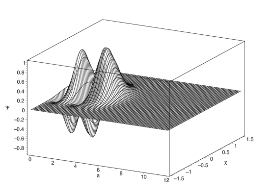
Figure 2: The vacuum wave function ($\zeta=0$) in the $a-\chi$ space with $\varepsilon_{r}=15$. (Only the mode $\chi_{n}$ with $n=10$ is shown, and other modes $\chi_{n}$ are omitted.) Oscillatory behavior until the turning point $a_{1}\approx 4$ is followed by an exponential decay under the barrier ($a>a_{1}$).

We now consider the wave function for a squeezed state with $\zeta\equiv\zeta\left(a_{1}\right)\neq 0$. We can construct the exact wave function using Eqs. (25), (43) and compare it with the Gaussian solution.

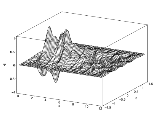
Figure 3: The wave function of a squeezed state ($\zeta=0.5$) in the $a-\chi$ space, with the same parameters as in Fig. 2. The underbarrier ($a>a_{1}$) wave function is dominated by highly excited states.

An explicit calculation of the exact wave function $\Psi\left(a,\chi_{n}\right)$ is given in Appendix A. At $a=a_{1}$ it has the form of a squeezed state with a squeezing parameter $\zeta\equiv\zeta\left(a_{1}\right)$. For $\zeta$ not too close to $1$, the wave function is dominated by the vacuum state and nearby states with low occupation numbers. However, as we go under the barrier, the contribution of highly excited states becomes increasingly important, and at large enough $a$ they completely dominate the wave function. This happens when $a$ exceeds the following $\zeta$-dependent bound,

$$a>a_{\max}\left(\zeta\right)\equiv\frac{\sqrt{\varepsilon_{r}}}{2}\left(\zeta^{-\frac{1}{2n}}+\zeta^{\frac{1}{2n}}\right).$$ (49)

These excited states belong to different semiclassical branches of the wave function, and thus the picture of a quantum field in a semiclassical background spacetime does not apply. The wave functions of the excited states exhibit short-wavelength oscillations in the $\chi$-direction, which are clearly visible in Fig. 3. This signals the breakdown of the Gaussian approximation. Now, it can be easily verified that the value $a_{\max}$ in Eq. (49) coincides with $a_{*}$ defined in Eq. (47) as the value of $a$ where $S_{n}\left(a\right)$ changes sign. This follows from (47) after substitution of the expression

$$\tau\left(a\right)=\cosh^{-1}\frac{a}{\sqrt{\varepsilon_{r}}}$$ (50)

for the Euclidean conformal time for $H=0$. If $\zeta\neq 0$ then $a_{\max}$ is finite and $Re\,S_{n}\left(a\right)$ becomes negative for $a>a_{\max}$. Only if $\zeta=0$, the condition of Eq. (19) holds for all $a>0$. We find that Eq. (19) is indeed the condition of consistency of the Gaussian approximation.

We wish to stress that the constant parameter $\zeta\equiv\zeta(a_{1})$ employed in the Appendix is not to be confused with the instantaneous squeezing parameter $\zeta\left(a\right)$ defined by Eq. (31). The instantaneous squeezing parameter $\zeta\left(a\right)$ does not necessarily reflect the true particle content of the quantum state. In particular, $\left|\zeta\left(a\right)\right|>1$ when $Re\,S_{n}\left(a\right)<0$, and a squeezed state with $\left|\zeta\right|>1$ is ill-defined and formally resembles a state with infinitely many particles, $\left\langle N\right\rangle=\infty$. The interpretation of Ref. R84 would suggest a “catastrophic particle production” due to tunneling if the barrier is wide enough so that $a_{2}>a_{\max}$. But, in fact, the model with a massless conformally coupled scalar field does not have any particle production.

A physical explanation of this result has already been partially given in Ref. R84 . A squeezed state is a superposition of all excited states, and the amplitudes of high-energy excited states are exponentially suppressed. On the other hand, the low-energy states contribute an exponentially suppressed amount to the wave function because of tunneling. But the two exponential suppression factors have a different behavior because the exponential suppression of low-energy states is $a$-dependent. Therefore, the high-energy states (which were already contained in the recollapsing universe) will give a dominant contribution to the wave function at large enough $a$ under the barrier.

IV Discussion

We have examined the solutions of the Wheeler-DeWitt equation for the FRW universe with a conformally coupled massless scalar field. We have shown that the wave function under the barrier exhibits all the signs of a “catastrophic particle production” in the sense of Rubakov et al., even though there is no actual particle production in this model. The calculations of Rubakov et al. are formally correct, but we disagree with their interpretation.

The wave function of the universe is a superposition of different semiclassical geometries; each semiclassical universe contains a different quantum state of the scalar field. If the quantum state of the universe is a superposition of low-energy and high-energy states of the scalar field, then the wave function of the expanding universe will be dominated by the semiclassical geometries that essentially did not tunnel, rather than by the geometry of an inflating universe created by tunneling.

For example, in the massless model we might consider a quantum state of the universe which is a superposition of the vacuum state $\Psi_{0}$ and of the state $\Psi_{n}^{k}$ which is the $k$-th excited state of a single mode $\chi_{n}$ of the quantum field. A superposition of these states such as $\Psi_{0}+\alpha\Psi_{n}^{k}$, with a small amplitude $\alpha$, will be close to the vacuum state to the left of the barrier (in the recollapsing universe). However, to the right of the barrier the contribution of the state $\Psi_{n}^{k}$ will dominate the wave function, and the inflating universe will appear to be in an excited state with the occupation number $k$ in the mode $\chi_{n}$.

This result should be interpreted not as a production of particles during tunneling, but rather as an emergence of excited states that have been already present in the recollapsing universe and became dominant in the expanding regime after tunneling. Had these highly excited states not been present, the final state would have been that of an empty inflating universe. Thus, to investigate the creation of the universe through quantum tunneling, the initial state of the recollapsing universe must be chosen correctly.

In the model with a conformally coupled massless scalar field, there is a preferred choice of the quantum state of the recollapsing universe which does not contain any admixture of excited states. This quantum state can be identified with the vacuum state. We have performed an explicit calculation to demonstrate that the wave function of any (non-vacuum) squeezed state becomes dominated by high-energy states exactly at the same region where the perturbative formalism of Rubakov et al. starts to break down.

We have also shown that the Gaussian solution of the Wheeler-DeWitt equation [Eq. (13)] is equivalent to a squeezed vacuum state in the formalism of Rubakov et al. The Gaussian solution also manifests the domination by high-energy states, in that the wave function starts to grow at large $\chi$. Therefore, the condition (19) that the Gaussian wave function decreases at large $\chi$ can be used to select a quantum state of the universe which is dominated by the vacuum state rather than by the admixture of high-energy excited states.

In the companion paper JVW2 , we shall extend our conclusions to the more general case of a massive conformally coupled field where, unlike the case of the massless field, one would expect some particle creation. We shall demonstrate that the quantum state of the recollapsing universe can be chosen to contain a sufficiently small admixture of excited states, and that in this case the WKB approximation is everywhere applicable and the backreaction of the matter excitations on the metric is negligible. We note that the under-barrier behavior of a massive field has been discussed by Bouhmadi-López, Garay and González-Díaz BGG02 , who constructed a vacuum wave function satisfying the condition of Eq. (19) in the case of a negative cosmological constant ($H^{2}<0$). The paper BGG02 has a significant overlap with our work in JVW2 , and we shall comment on it there in more detail.

Appendix A The under-barrier wave function of a squeezed state

Here we compute the wave function of a squeezed state with an arbitrary squeezing parameter $\zeta\neq 0$ in the case $H=0$. The potential $V\left(a\right)$ is

$$V\left(a\right)=a^{2}-\varepsilon_{r}.$$ (51)

For simplicity we consider the vacuum state in all modes except one particular mode $\chi_{n}$. [Simultaneous squeezed states of several modes give analogous results.] Our purpose is to show that the wave function under the barrier is dominated by the contribution of certain high-energy excited states, rather than by the vacuum solution, and to find the relevant range of $a$.

For an excited state of the mode $\chi_{n}$ with occupation number $2k$, the turning point is at

$$a_{0}\left(2k\right)=\sqrt{\varepsilon_{r}+4n\hbar k}.$$ (52)

For a given $a$, excited states with $k>k_{\min}\left(a\right)$ are above the barrier, where

$$k_{\min}=\frac{V\left(a\right)}{4n\hbar}.$$ (53)

The wave function for an excited state of level $2k$ is [cf. Eq. (20)]

$$\Psi_{2k}\left(a,\chi_{n}\right)=\left(\frac{n}{\pi\hbar}\right)^{\frac{1}{4}}\frac{H_{2k}\left(\chi_{n}\sqrt{\frac{n}{\hbar}}\right)}{\sqrt{\left(4k\right)!!}}\exp\left(-\frac{n\chi_{n}^{2}}{2\hbar}\right)\psi_{2k}\left(a\right),$$ (54)

where the $a$-dependent part $\psi_{2k}\left(a\right)$ is given by a WKB approximation,

$$\psi_{2k}\left(a\right)\propto\left\{\begin{array}[]{l}\frac{1}{\sqrt[4]{V\left(a\right)-4n\hbar k}}\exp\left(-\frac{1}{\hbar}\int_{a_{0}\left(2k\right)}^{a}\sqrt{V\left(a\right)-4n\hbar k}\,da\right),\quad a>a_{0}\left(2k\right),\\ \frac{2}{\sqrt[4]{4n\hbar k-V\left(a\right)}}\cos\left(\frac{1}{\hbar}\int_{a}^{a_{0}\left(2k\right)}\sqrt{4n\hbar k-V\left(a\right)}\,da-\frac{\pi}{4}\right),\quad 0<a<a_{0}\left(2k\right).\end{array}\right.$$ (55)

The wave function $\Psi\left(a,\left\{\chi_{l}\right\}\right)$ is a superposition of the wave functions for excited states of the mode $\chi_{n}$ (we suppress the dependence on other modes $\chi_{l}$ with $l\neq n$), with coefficients given by Eq. (25) with the squeezing parameter $\zeta$,

$$\Psi\left(a,\chi_{n}\right) = \left(1-\left|\zeta\right|^{2}\right)^{\frac{1}{4}}\left(\frac{n}{\pi\hbar}\right)^{\frac{1}{4}}\exp\left(-\frac{n\chi_{n}^{2}}{2\hbar}\right)$$ (56)

$$\times\sum_{k=0}^{\infty}\frac{\left(-\zeta\right)^{k}\sqrt{\left(2k\right)!}}{2^{k}k!}\frac{H_{2k}\left(\chi_{n}\sqrt{\frac{n}{\hbar}}\right)}{\sqrt{\left(4k\right)!!}}\psi_{2k}\left(a\right).$$

For the analysis below we will need an asymptotic formula for Hermite polynomials $H_{n}\left(x\right)$ at fixed $x$ and large $n$,

$$H_{n}\left(x\right)\sim\sqrt{2}\left(2n\right)^{\frac{n}{2}}e^{\frac{x^{2}}{2}-\frac{n}{2}+O(n^{-1})}\cos\left(-\frac{\pi n}{2}+x\sqrt{2n}+O(n^{-1/2})\right).$$ (57)

This expression can be derived by the method of steepest descent from the integral representation (cf. AS64 , Eq. 22.10.15)

$$H_{n}\left(x\right)=\frac{i^{n}}{2\sqrt{\pi}}\int_{-\infty}^{+\infty}e^{-\left(\frac{t}{2}+ix\right)^{2}}t^{n}dt.$$ (58)

Using the Stirling formula for large factorials

$$n!\sim\sqrt{2\pi n}\left(\frac{n}{e}\right)^{n}(1+O\left(n^{-1}\right)),$$ (59)

we find

$$\frac{\sqrt{\left(2k\right)!}}{2^{k}k!}\sim k^{-1/4}.$$ (60)

Compared with the exponential functions of $k$ in Eq. (56), this is a slowly changing factor.

Consider the contribution of the state $\left|2k\right\rangle$ to the wave function, as a function of $k$. The contribution of levels $k>k_{\min}$ decreases with $k$ because of the suppression factor $\zeta^{k}$. The absolute value of the contribution of a level $k<k_{\min}$ can be estimated as

$$\left|\zeta^{k}\Psi_{2k}\left(a,\chi_{n}\right)\right|\sim\exp\left(-zk-\frac{1}{\hbar}\int_{a_{0}\left(2k\right)}^{a}\sqrt{V\left(a\right)-4n\hbar k}\,da\right).$$ (61)

Here we have defined for convenience

$$z\equiv-\ln\left|\zeta\right|.$$ (62)

[We have used the asymptotic Eq. (57) which is justified if $k$ is large. There is no dependence on $\chi_{n}$ in the absolute value of the wave function.] For $V\left(a\right)$ given by Eq. (51), the integral in Eq. (61) can be evaluated as

$$\int_{a_{0}}^{a}\sqrt{a^{2}-a_{0}^{2}}\,da=\frac{a}{2}\sqrt{a^{2}-a_{0}^{2}}-\frac{a_{0}^{2}}{2}\cosh^{-1}\frac{a}{a_{0}}.$$ (63)

The function under the exponential in Eq. (61) has a maximum at

$$k=k_{0}\left(a,\zeta\right)=\frac{1}{4n\hbar}\left(\frac{a^{2}}{\cosh^{2}\frac{z}{2n}}-\varepsilon_{r}\right).$$ (64)

[Note that $k_{0}>0$ only for large enough $a$.] Therefore the dominant contribution to the wave function comes from either $k=0$ (for $0<a<\sqrt{\varepsilon_{r}}\cosh\frac{z}{2n}$) or from $k\approx k_{0}\left(a,\zeta\right)$ (for $a>\sqrt{\varepsilon_{r}}\cosh\frac{z}{2n}$). One can see this in Fig. 3: at progressively larger values of $a$, the wave function exhibits more oscillations in the $\chi_{n}$ direction, which corresponds to excited states with different values of $k=k_{0}\left(a,\zeta\right)$.

We find that the wave function $\Psi\left(a,\chi_{n}\right)$ is dominated by the contribution of excited states $\Psi_{2k}$ with $k\approx k_{0}\left(a,\zeta\right)$ when

$$a>a_{\max}\equiv\sqrt{\varepsilon_{r}}\cosh\frac{z}{2n}=\frac{\sqrt{\varepsilon_{r}}}{2}\left(\zeta^{-\frac{1}{2n}}+\zeta^{\frac{1}{2n}}\right).$$ (65)

This is the expression we needed in Sec. III.3.

References

- (1) A. Vilenkin, Phys. Rev. D 30, 509 (1984); 33, 3560 (1986).
- (2) V. A. Rubakov, Phys. Lett. B 148, 280 (1984).
- (3) Y. B. Zeldovich and A. A. Starobinsky, Sov. Astron. Lett. 10, 135 (1984).
- (4) J. B. Hartle and S. W. Hawking, Phys. Rev. D 28, 2960 (1983).
- (5) A. D. Linde, Lett. Nuovo Cim. 39, 401 (1984).
- (6) A. Vilenkin, preprint gr-qc/0204061 (2002).
- (7) D. Levkov, C. Rebbi, and V. A. Rubakov, preprint gr-qc/0206028 (2002).
- (8) A. Vilenkin, Phys. Rev. D 37, 888 (1988).
- (9) T. Vachaspati and A. Vilenkin, Phys. Rev. D 37, 898 (1988).
- (10) J. Garriga and A. Vilenkin, Phys. Rev. D 56, 2464 (1997).
- (11) L. Parker, Phys. Rev. 183, 1057 (1969).
- (12) J. Hong, A. Vilenkin, and S. Winitzki, in preparation.
- (13) J. J. Halliwell and S. W. Hawking, Phys. Rev. D 31, 1777 (1985).
- (14) V. Lapchinsky and V. A. Rubakov, Acta Phys. Pol. B 10, 1041 (1979).
- (15) T. Banks, Nucl. Phys. B 249, 332 (1985).
- (16) T. Banks, C. Bender, and T. T. Wu, Phys. Rev. D 8, 3346 (1973); 8, 3366 (1973).
- (17) N. D. Birrell and P. C. W. Davies, Quantum fields in curved space, Cambridge University Press, Cambridge, 1982.
- (18) S. A. Fulling, Gen. Rel. Grav. 10, 807 (1979).
- (19) M. Abramowitz and I. A. Stegun, Handbook of Mathematical Functions, National Bureau of Standards, 1964.
- (20) M. Bouhmadi-López, L. J. Garay, and P. F. González-Díaz, preprint astro-ph/0204072 (2002).