Geodesics in spacetimes with expanding impulsive gravitational waves

Abstract

We study geodesic motion in expanding spherical impulsive gravitational waves propagating in a Minkowski background. Employing the continuous form of the metric we find and examine a large family of geometrically preferred geodesics. For the special class of axially symmetric spacetimes with the spherical impulse generated by a snapping cosmic string we give a detailed physical interpretation of the motion of test particles.

I Introduction

In his classical work Pen72 Roger Penrose constructed impulsive spherical gravitational waves in a Minkowski background using his vivid “cut and paste” method. It is based on cutting the spacetime along a null cone and then re-attaching the two pieces with a suitable warp. An explicit solution using coordinates in which the metric is continuous was later on given by Nutku and Penrose NutPen92 and Hogan Hogan93 ; Hogan94 , but was only recently related explicitly to the impulsive limit of Robinson–Trautman type N  solutions PodGri99 ; GriPodDoc02 . However, the latter has to be considered as only formal since the metric tensor contains terms proportional to the square of the Dirac-$\delta$, and the transformation relating this coordinate system to the continuous one mentioned above is necessarily discontinuous. Nevertheless, this transformation is analogous to the one relating the distributional and the continuous form of the metric tensor for impulsive pp -waves (plane-fronted gravitational waves with parallel rays kramerbook ) which was also introduced in Pen72 and has recently been analyzed rigorously  Stein98 ; KunSt99 using nonlinear theories of generalized functions (Colombeau algebras) Col84 ; Col92 . It is thus a natural open question whether a similar mathematically sound treatment can also be found for expanding spherical impulses. This indeed is one main motivation for the present work in which we study the motion of test particles in spacetimes with spherical impulsive waves.

On the other hand this work is motivated by the quest of a physical interpretation of radiative Robinson–Trautman spacetimes, one of the most interesting non-static exact solutions of Einstein’s equations which admit a geodesic, shearfree and twistfree null congruence of diverging rays kramerbook . This large family involves not only spacetimes of Petrov type N  (investigated in the impulsive limit in the present paper) but also type II  solutions describing bodies which radiate away their asymmetries and approach a Schwarzschild black hole, or the $C$-metric of type D  which represents gravitational radiation generated by uniformly accelerated black holes. By studying these explicit exact solutions one may acquire an intuition necessary for investigation of more general and realistic situations.

This work is organized as follows. In Sec. II we review the class of spacetimes under consideration and describe the geometry of the expanding impulses. By employing the continuous form of the metric in Sec. III we find a large class of privileged and simple geodesics which can be related to explicit geodesics in the distributional form of the metric “in front” and “behind” the spherical impulse. This may allow one to lay the foundations for a rigorous (distributional) treatment of impulsive Robinson–Trautman solutions of type N  as well as the transformation relating the latter to the continuous form of the metric. Moreover, assuming the geodesics to be $C^{1}$ across the impulse (in the continuous system) we completely solve the problem of geodesic motion in spacetimes with expanding impulsive gravitational waves. In Sec. IV we focus on impulsive waves generated by a snapping cosmic string. This interesting solution of Einstein’s equations was previously constructed by Gleiser and Pullin GlePul89 and Nutku and Penrose NutPen92 using the “cut and paste” method. An independent approach was used by Bičák Bicak90 ; BicSch89 (with recent generalizations in PodGri01a ) who obtained the same spacetime by considering a null limit of particular solutions with boost-rotational symmetry representing a pair of particles uniformly accelerating due to semi-infinite strings attached to them. We discuss in detail the physical interpretation of the motion of test particles influenced by such an impulse.

II Expanding impulsive waves in a Minkowski background

As mentioned above, Penrose Pen72 has described a “cut and paste” method for constructing expanding spherical gravitational waves in a Minkowski background. The procedure can be performed explicitly as follows. One starts with the Minkowski line element

$${\rm d}s_{0}^{2}=2\,{\rm d}\eta\,{\rm d}\bar{\eta}-2\,{\rm d}{\cal U}\,{\rm d}{\cal V}=-{\rm d}t^{2}+{\rm d}x^{2}+{\rm d}y^{2}+{\rm d}z^{2}\,,$$ (1)

where the relation between the coordinates is given by

$${\cal U}=\textstyle{\frac{1}{\sqrt{2}}}(t+z)\ ,\ {\cal V}=\textstyle{\frac{1}{\sqrt{2}}}(t-z)\ ,\ \eta=\textstyle{\frac{1}{\sqrt{2}}}(x+\,\hbox{i}\,y)\ .$$ (2)

We may now perform the transformation

$${\cal V} = \frac{V}{p}-\epsilon U\ ,$$

$${\cal U} = \frac{Z\bar{Z}}{p}\,V-U\ ,$$ (3)

$$\eta = \frac{Z}{p}\,V\ ,$$

where

$$p=1+\epsilon Z\bar{Z}\ ,\qquad\epsilon=-1,0,+1\ .$$ (4)

(The parameter $\epsilon$ is related to the Gaussian curvature of the 2-surfaces given by $U=$ const.  $V=$ const., cf. PodGri99 .) Using (3), the metric (1) takes the form

$${\rm d}s_{0}^{2}=2\frac{V^{2}}{p^{2}}\,{\rm d}Z\,{\rm d}\bar{Z}+2\,{\rm d}U\,{\rm d}V-2\epsilon\,{\rm d}U^{2}\ .$$ (5)

On the other hand, we consider the alternative, more involved transformation given by

$${\cal V} = AV-DU\ ,$$

$${\cal U} = BV-EU\ ,$$ (6)

$$\eta = CV-FU\ ,$$

where

$$A=\frac{1}{p|h^{\prime}|}\ ,\qquad B=\frac{|h|^{2}}{p|h^{\prime}|}\ ,\qquad C=\frac{h}{p|h^{\prime}|}\ ,$$

$$D=\frac{1}{|h^{\prime}|}\left\{\frac{p}{4}\left|\frac{h^{\prime\prime}}{h^{\prime}}\right|^{2}+\epsilon\left[1+\frac{Z}{2}\frac{h^{\prime\prime}}{h^{\prime}}+\frac{\bar{Z}}{2}\frac{\bar{h}^{\prime\prime}}{\bar{h}^{\prime}}\right]\right\}\ ,$$

$$E=\frac{|h|^{2}}{|h^{\prime}|}\bigg{\{}\frac{p}{4}\left|\frac{h^{\prime\prime}}{h^{\prime}}-2\frac{h^{\prime}}{h}\right|^{2}$$

$$\qquad+\epsilon\left[1+\frac{Z}{2}\left(\frac{h^{\prime\prime}}{h^{\prime}}-2\frac{h^{\prime}}{h}\right)+\frac{\bar{Z}}{2}\left(\frac{\bar{h}^{\prime\prime}}{\bar{h}^{\prime}}-2\frac{\bar{h}^{\prime}}{\bar{h}}\right)\right]\bigg{\}}\ ,$$

$$F=\frac{h}{|h^{\prime}|}\bigg{\{}\frac{p}{4}\left(\frac{h^{\prime\prime}}{h^{\prime}}-2\frac{h^{\prime}}{h}\right)\frac{\bar{h}^{\prime\prime}}{\bar{h}^{\prime}}$$

$$\qquad+\epsilon\left[1+\frac{Z}{2}\left(\frac{h^{\prime\prime}}{h^{\prime}}-2\frac{h^{\prime}}{h}\right)+\frac{\bar{Z}}{2}\frac{\bar{h}^{\prime\prime}}{\bar{h}^{\prime}}\right]\bigg{\}}\ .$$ (7)

Here $h\equiv h(Z)$ is an arbitrary function, and the derivative with respect to its argument $Z$ is denoted by a prime. With this, the Minkowski metric (1) becomes

$${\rm d}s_{0}^{2}=2\left|\frac{V}{p}\,{\rm d}Z+U\,p\,\bar{H}\,{\rm d}\bar{Z}\right|^{2}+2\,{\rm d}U\,{\rm d}V-2\epsilon\,{\rm d}U^{2}\ ,$$ (8)

where $H$ is the Schwarzian derivative of $h$, i.e.,

$$H(Z)=\frac{1}{2}\left[\frac{h^{\prime\prime\prime}}{h^{\prime}}-\frac{3}{2}\left(\frac{h^{\prime\prime}}{h^{\prime}}\right)^{2}\right].$$ (9)

In the coordinates used in (5) as well as in the ones used in (8), the null hypersurface  $U=0$  represents a null cone $\eta\bar{\eta}-{\cal U}{\cal V}=0$, i.e., an expanding sphere $x^{2}+y^{2}+z^{2}=t^{2}$ in the Minkowski background. Moreover, the reduced 2-metrics on this cone are identical. Following the Penrose “cut and paste” method, we attach the line element (5) for $U<0$ to (8) for $U>0$. The resulting metric takes the form

$${\rm d}s^{2}=2\left|\frac{V}{p}\,{\rm d}Z+U\Theta(U)\,p\,\bar{H}\,{\rm d}\bar{Z}\right|^{2}\!\!+2\,{\rm d}U\,{\rm d}V-2\epsilon\,{\rm d}U^{2}\,,$$ (10)

where $\Theta(U)$ is the Heaviside step function. This combined metric, which was first presented in NutPen92 ; Hogan94 , is explicitly continuous everywhere, including the null hypersurface $U=0$. However, the discontinuity in the derivatives of the metric across $U=0$ yields an impulsive gravitational wave term proportional to the Dirac $\delta$-function. More precisely, the only non-vanishing component of the Weyl tensor in the Newman-Penrose formalism np ; kramerbook is $\Psi_{4}=(p^{2}H/V)\,\delta(U)$ which is the component $\Psi_{4}\equiv C_{abcd}l^{a}\bar{m}^{b}l^{c}\bar{m}^{d}$ with respect to the null tetrad ${\bf k}=\partial_{V}$, ${\bf l}=-\epsilon\,\partial_{V}-\partial_{U}$, ${\bf m}=p^{2}(V^{2}-U^{2}\Theta\,p^{4}H\bar{H})^{-1}[(V/p)\,\partial_{\bar{Z}}-U\Theta\,p\,\bar{H}\,\partial_{Z}]$. The spacetime is thus flat everywhere except on the wave surface $U=0$. Also, as shown in PodGri00 , the only non-vanishing tetrad component of the Ricci tensor is $\Phi_{22}\equiv\frac{1}{2}R_{ab}l^{a}l^{b}=(p^{4}H\bar{H}/V^{2})\,U\delta(U)$. This demonstrates that the spacetime is vacuum everywhere (except on the impulse at $V=0$ and at possible singularities of the function $p^{2}H$).

For later use we also remark that the inverse relation to (3) is given by

$$U=\frac{\eta\bar{\eta}}{{\cal V}}-{\cal U}\ ,$$

$$V={\cal V}\ ,$$ (11)

$$Z=\frac{\eta}{{\cal V}}\ ,$$

when $\epsilon=0$, and by

$$U=-\epsilon{\cal V}-\frac{2\eta\bar{\eta}}{({\cal V}-\epsilon{\cal U})\mp\sqrt{({\cal V}-\epsilon{\cal U})^{2}+4\epsilon\eta\bar{\eta}}}\ ,$$

$$V=-({\cal V}-\epsilon{\cal U})-\frac{4\epsilon\eta\bar{\eta}}{({\cal V}-\epsilon{\cal U})\mp\sqrt{({\cal V}-\epsilon{\cal U})^{2}+4\epsilon\eta\bar{\eta}}}\ ,$$

$$Z=-\frac{\epsilon}{2\bar{\eta}}\left[({\cal V}-\epsilon{\cal U})\mp\sqrt{({\cal V}-\epsilon{\cal U})^{2}+4\epsilon\eta\bar{\eta}}\,\right]\ ,$$ (12)

for $\epsilon\not=0$.

We may define the functions $U_{inv}$, $V_{inv}$ and $Z_{inv}$ of $(U,V,Z,\bar{Z})$ as the composition of (11) (or (12) for $\epsilon\not=0$) with (6), (7), which transforms the metric (8) to (5). Consequently, a discontinuous transformation

$$u = U+\Theta(U)\,[\,U_{inv}(U,V,Z,\bar{Z})-U\,]\ ,$$

$$w = V+\Theta(U)\,[\,V_{inv}(U,V,Z,\bar{Z})-V\,]\ ,$$ (13)

$$\xi = Z+\Theta(U)\,[\,Z_{inv}(U,V,Z,\bar{Z})-Z\,]\ ,$$

relates (10) for all $U\not=0$ to Minkowski spacetime in the form

$${\rm d}s_{0}^{2}=2\frac{w^{2}}{\psi^{2}}\,{\rm d}\xi\,{\rm d}\bar{\xi}+2\,{\rm d}u\,{\rm d}w-2\epsilon\,{\rm d}u^{2}\ ,$$ (14)

where $\psi=1+\epsilon\xi\bar{\xi}$. Interestingly, by considering the transformation (13) of the metric (10) for arbitrary $U$, i.e., keeping also the distributional terms, one (formally) obtains the metric

$${\rm d}s^{2} = 2\frac{w^{2}}{\psi^{2}}\left|{\rm d}\xi-f\,\delta(u){\rm d}u\,\right|^{2}+2\,{\rm d}u\,{\rm d}w-2\epsilon\,{\rm d}u^{2}$$ (15)

$$\!\!+w\Big{[}(f_{\xi}+\bar{f}_{\bar{\xi}})-\frac{2\epsilon}{\psi}(f\bar{\xi}+\bar{f}\xi)\Big{]}\delta(u){\rm d}u^{2}\ ,$$

in which $f(\xi)$ is related to $h(Z)$ through the identification $f\equiv Z_{inv}-Z$ evaluated on $U=0$. Although this form of the metric is only formal since it contains the square of the delta function, it explicitly shows that expanding impulsive gravitational waves (10) arise as the impulsive limits of the Robinson–Trautman type N  spacetimes, expressed in the coordinates introduced in GarPle81 (see BicPod99 ; PodGri99 for the details).

Let us now conclude this review section by a brief description of the geometry of the above expanding impulsive waves localized along the wave-surfaces $U=0$, i.e., $u=0$. This will also elucidate the meaning of the parameter $\epsilon$.

From the Robinson–Trautman form of the metric (15) it is obvious that the impulse splits the spacetime into two flat regions, $u>0$ and $u<0$. In the following we shall call the Minkowski half-space $u>0$ as being “in front of the wave”, and the other Minkowski half-space $u<0$ (note that $u\equiv U$ for $U<0$) as being “behind the wave”. The “background” metric on both sides of the impulse is given by (14). For arbitrary  $u\not=0$, this metric can be put into explicit Minkowski form (1) by the transformations (2) and (11) (or (12)) and the (trivial) identification $u=U$, $w=V$, $\xi=Z$. Using these relations, we can easily analyze the geometry of the null hypersurfaces $u=u_{0}=$const. in Minkowski coordinates which are geometrically privileged and thus allow for a clear physical interpretation.

We start with the subclass of solutions for which $\epsilon=0$. Substituting (2) into (11) and setting $U=u_{0}$, we get the relation

$$x^{2}+y^{2}+(z+{\textstyle\frac{1}{\sqrt{2}}}\,u_{0}\,)^{2}=(t+{\textstyle\frac{1}{\sqrt{2}}}\,u_{0}\,)^{2}$$ (16)

(if $t\not=z$, i.e., for $x\not=0$, $y\not=0$). For various values of $u_{0}$ this represents a family of null cones with vertices at $(-{\textstyle\frac{1}{\sqrt{2}}}\,u_{0},0,0,-{\textstyle\frac{1}{\sqrt{2}}}\,u_{0}\,)$ localized along a singular null line $t=z,x=0,y=0$. Also, $V=w_{0}=\,$const. is a set of parallel hyperplanes $t=z+\sqrt{2}\,w_{0}$ in the Minkowski background. This reveals the geometrical meaning of the coordinates $u,w$ used in the metric (14) with $\epsilon=0$. Note that $w=0$ represents a physical singularity in the Robinson–Trautman spacetimes BicPra98 which can be interpreted as the source of the wave surfaces $u=u_{0}$. At any time $t$, these surfaces are spheres of the radius $R=|t+{\textstyle\frac{1}{\sqrt{2}}}\,u_{0}|$. In particular, the impulse localized on $u=0$ is a null cone with the vertex in the origin which, at any time, is a sphere of radius $R=\sqrt{x^{2}+y^{2}+z^{2}}=|t|$.

Analogous results can similarly be obtained for the remaining two subclasses $\epsilon=\pm 1$. In this case, using (2) and (12), the hypersurfaces $u_{0}$=const. are given by

$$x^{2}+y^{2}+z^{2}=(t+\sqrt{2}\,u_{0})^{2}\ ,$$ (17)

for $\epsilon=+1$ and

$$x^{2}+y^{2}+(z+\sqrt{2}\,u_{0})^{2}=t^{2}\ ,$$ (18)

for $\epsilon=-1$, respectively. Again, these are families of null cones in Minkowski space with vertices shifted in the $t$-direction for $\epsilon=+1$, and in the $z$-direction for $\epsilon=-1$. Note that these vertices form a singular timelike line $x=0=y$, $z=0$ if $\epsilon=+1$, and a spacelike line $x=0=y$, $t=0$ if $\epsilon=-1$. These lines are given by $\eta=0$, ${\cal V}-\epsilon{\cal U}=0$, and correspond to the physical singularity of the Robinson–Trautman spacetime at $w=0$.

It is obvious that for the above spacetimes with a single expanding impulsive wave localized at $u=u_{0}=0$, i.e., at $U=0$, the null cones of the three classes of wave-surfaces given by (16), (17), and (18) coincide. In fact, in the impulsive limit the three (generically different) subclasses $\epsilon=0,+1,-1$ of the Robinson–Trautman class of solutions are locally equivalent PodGri99 .

It can also be observed, that for $\epsilon=0$, the physical singularity at $V=0$ is a singular null line on the wavefront surface $U=0$. For a physical interpretation, it would be better to remove this singularity from the spacetime. This can be achieved by considering solutions with $\epsilon\neq 0$: In these cases, the singularity at $V=0$ appears only at the vertex of the null cone, $x=y=z=t=0$, which may be considered as the “origin” of the spherical wave.

III Geodesic motion in spacetimes with expanding impulsive waves

The purpose of this paper is to investigate the effect of expanding impulsive waves of Robinson–Trautman type on the motion of freely moving test particles. It is natural to start with geodesics in (local, see below) Minkowski space $U>0$ in front of the wave, i.e., “outside” the null cone $U=0$ corresponding to $x^{2}+y^{2}+z^{2}=t^{2}$. (Note that at $t=0$ the spherical impulse is just “created” at the origin.) Obviously, general geodesics are given by

$$t^{+}=\gamma\,\tau\ ,$$

$$x^{+}=\dot{x}_{0}\,(\tau-\tau_{i})+x_{0}\ ,$$ (19)

$$y^{+}=\dot{y}_{0}\,(\tau-\tau_{i})+y_{0}\ ,$$

$$z^{+}=\dot{z}_{0}\,(\tau-\tau_{i})+z_{0}\ ,$$

with $\gamma=\sqrt{\dot{x}_{0}^{2}+\dot{y}_{0}^{2}+\dot{z}_{0}^{2}-e}$, i.e., $\tau$ is a normalized affine parameter of timelike ($e=-1$) or spacelike ($e=+1$) geodesics. For null geodesics ($e=0$) it is always possible to scale the factor $\gamma$ to unity. The constants $x_{0},y_{0},z_{0}$ and $\dot{x}_{0},\dot{y}_{0},\dot{z}_{0}$ characterize position resp. velocity of each test particle at the instant

$$\tau_{i}=\sqrt{x_{0}^{2}+y_{0}^{2}+z_{0}^{2}}\,/\,\gamma\ ,$$ (20)

when the geodesic intersects the null cone. At $\tau_{i}$ each particle is hit by the impulse and its trajectory is refracted and (possibly) shifted. The geodesics (19) in front of the impulse can also be written as

$${\cal V}^{+} = \dot{\cal V}_{0}^{+}(\tau-\tau_{i})+{\cal V}_{0}^{+}\ ,$$

$${\cal U}^{+} = \dot{\cal U}_{0}^{+}(\tau-\tau_{i})+{\cal U}_{0}^{+}\ ,$$ (21)

$$\eta^{+} = \dot{\eta}_{0}^{+}(\tau-\tau_{i})+\eta_{0}^{+}\ ,$$

where

$$\dot{\cal V}_{0}^{+}=\textstyle{\frac{1}{\sqrt{2}}}(\gamma-\dot{z}_{0})\ ,\quad\ {\cal V}_{0}^{+}=\textstyle{\frac{1}{\sqrt{2}}}(\gamma\tau_{i}-z_{0})\ ,$$

$$\dot{\cal U}_{0}^{+}=\textstyle{\frac{1}{\sqrt{2}}}(\gamma+\dot{z}_{0})\ ,\quad\ {\cal U}_{0}^{+}=\textstyle{\frac{1}{\sqrt{2}}}(\gamma\tau_{i}+z_{0})\ ,$$ (22)

$$\dot{\eta}_{0}^{+}=\textstyle{\frac{1}{\sqrt{2}}}(\dot{x}_{0}+\hbox{i}\,\dot{y}_{0})\ ,\quad\eta_{0}^{+}=\textstyle{\frac{1}{\sqrt{2}}}(x_{0}+\hbox{i}\,y_{0})\ .$$

Now, we wish to investigate the influence of the impulse on the geodesics, and to determine explicitly formulae for corresponding “refraction” and “shift”. In the region $U<0$ behind the impulse the particles again move in Minkowski space (1) so that the trajectories also have to be straight lines of the form

$${\cal V}^{-} = \dot{\cal V}_{0}^{-}(\tau-\tau_{i})+{\cal V}_{0}^{-}\ ,$$

$${\cal U}^{-} = \dot{\cal U}_{0}^{-}(\tau-\tau_{i})+{\cal U}_{0}^{-}\ ,$$ (23)

$$\eta^{-} = \dot{\eta}_{0}^{-}(\tau-\tau_{i})+\eta_{0}^{-}\ .$$

It remains to express the constants appearing in (23) in terms of the initial data introduced in (19), and the structural function $h(Z)$, which characterizes specific expanding impulsive waves.

The key idea is to employ the continuous form of the solution (10). It can easily be observed that in this coordinate system the Christoffel symbols $\,\Gamma^{\mu}_{UU}$, $\Gamma^{\mu}_{UV}$, and $\Gamma^{\mu}_{VV}$ vanish identically. Therefore, the geodesic equations always admit privileged global solutions of the form

$$Z = Z_{0}=\hbox{const.}\ ,$$

$$U = \dot{U}_{0}(\tau-\tau_{i})\ ,$$ (24)

$$V = \dot{V}_{0}(\tau-\tau_{i})+V_{0}\ .$$

Here we have set $U_{0}=0$, so that each geodesic reaches the impulse localized at $U=0$ at parameter-time $\tau=\tau_{i}$.

Using (6), it is possible to express the geodesics (24) in front of the impulse in the Minkowski form (21) where the coefficients (22) are

$$\dot{\cal V}_{0}^{+}=A\dot{V}_{0}-D\dot{U}_{0}\ ,\quad{\cal V}_{0}^{+}=AV_{0}\ ,$$

$$\dot{\cal U}_{0}^{+}=B\dot{V}_{0}-E\dot{U}_{0}\ ,\quad{\cal U}_{0}^{+}=BV_{0}\ ,$$ (25)

$$\dot{\eta}_{0}^{+}\,=C\dot{V}_{0}-F\dot{U}_{0}\ ,\quad\>\eta_{0}^{+}=\,CV_{0}\ .$$

The constants $A,B,C,D,E$ and $F$ are given by the values of the functions (7) at $Z=Z_{0}$. The relations (22) and (25) enable us to relate the parameters $Z_{0}$, $\dot{U}_{0}$, $\dot{V}_{0}$, and $V_{0}$ to the natural initial data introduced in (19) by

$$x_{0}=\sqrt{2}\,\,V_{0}\,{\cal R}e\,C\ ,$$

$$y_{0}=\sqrt{2}\,\,V_{0}\,{\cal I}m\,C\ ,$$

$$z_{0}=\textstyle\frac{1}{\sqrt{2}}\,V_{0}\,(B-A)\ ,$$ (26)

$$\dot{x}_{0}=\sqrt{2}\,\,[\,\dot{V}_{0}\,{\cal R}e\,C-\dot{U}_{0}\,{\cal R}e\,F\,]\ ,$$

$$\dot{y}_{0}=\sqrt{2}\,\,[\,\dot{V}_{0}\,{\cal I}m\,C-\dot{U}_{0}\,{\cal I}m\,F\,]\ ,$$

$$\dot{z}_{0}=\textstyle\frac{1}{\sqrt{2}}\,[\,\dot{V}_{0}\,(B-A)-\dot{U}_{0}\,(E-D)\,]\ .$$

The three position parameters $x_{0}$, $y_{0}$, $z_{0}$ are thus related to the three independent constants $Z_{0}$, $\bar{Z}_{0}$, $V_{0}$. The normalization condition implies the constraint $(\dot{V}_{0}-\epsilon\dot{U}_{0})\dot{U}_{0}={\textstyle\frac{1}{2}}e$ (which can be obtained using the identities $AB-C\bar{C}=0$, $DE-F\bar{F}=\epsilon$, and $AE+BD-C\bar{F}-\bar{C}F=1$) on the parameters $\dot{V}_{0}$ and $\dot{U}_{0}$. However, in general it is possible to set at least one of the velocities $\dot{x}_{0}$, $\dot{y}_{0}$, or $\dot{z}_{0}$ to zero by a suitable choice of $\dot{U}_{0}$.

Finally, we transform the geodesics (24) behind the impulse using (3), which gives the uniform Minkowskian motion (23) with the coefficients

$$\dot{\cal V}_{0}^{-}=\frac{\dot{V}_{0}}{p}-\epsilon\dot{U}_{0}\ ,\quad\qquad{\cal V}_{0}^{-}=\frac{V_{0}}{p}\ ,$$

$$\dot{\cal U}_{0}^{-}=\frac{Z_{0}\bar{Z}_{0}}{p}\dot{V}_{0}-\dot{U}_{0}\ ,\quad{\cal U}_{0}^{-}=\frac{Z_{0}\bar{Z}_{0}}{p}V_{0}\ ,$$ (27)

$$\dot{\eta}_{0}^{-}=\frac{Z_{0}}{p}\dot{V}_{0}\ ,\qquad\qquad\quad\eta_{0}^{-}=\frac{Z_{0}}{p}V_{0}\ .$$

Substituting for $Z_{0}$, $V_{0}$, $\dot{V}_{0}$ and $\dot{U}_{0}$ from the inverse of the relations (26), we obtain an explicit result which can be used for discussion of the effect of expanding impulsive waves on the privileged family of geodesics (24).

However, it should be emphasized that in the above construction we started with the initial data (19) outside the impulse in the region $U>0$, which is a Minkowski space only locally. Due to the complicated form of the generating complex function $h$, there are topological defects such as cosmic strings (corresponding to the presence of deficit angles) outside the null cone, see e.g., PodGri00 for more details. Therefore, for better physical interpretation it may be useful to set the initial data for the geodesics in the region $U<0$ inside the cone, which is considered to be a “complete” Minkowski space without topological defects. Evolving these data,

$$t^{-}=\gamma\,\tau\ ,$$

$$x^{-}=\dot{x}_{0}\,(\tau-\tau_{i})+x_{0}\ ,$$ (28)

$$y^{-}=\dot{y}_{0}\,(\tau-\tau_{i})+y_{0}\ ,$$

$$z^{-}=\dot{z}_{0}\,(\tau-\tau_{i})+z_{0}\ ,$$

“backward” in time (i.e., for decreasing affine parameter $\tau$), it is possible to prolong the geodesics across the spherical impulse to the “incomplete” Minkowski region $U>0$ with cosmic strings outside the impulse.

In this case, the explicit geodesics outside the impulse have the form (21), (25), in which the constants $Z_{0}$, $V_{0}$, $\dot{V}_{0}$ and $\dot{U}_{0}$ have to be expressed in terms of the data (28). Using (11) for $\epsilon=0$, and (12) for $\epsilon\not=0$ we obtain

$$Z_{0}=\frac{x_{0}+\,\hbox{i}\,y_{0}}{\gamma\tau_{i}-z_{0}}\ ,$$

$$V_{0}={\textstyle\frac{1}{\sqrt{2}}}\,[(1+\epsilon)\gamma\tau_{i}-(1-\epsilon)z_{0}]\ ,$$

$$\dot{V}_{0}={\textstyle\frac{1}{\sqrt{2}}}\,[(1-\epsilon)\gamma-(1+\epsilon)\dot{z}_{0}]\,\frac{(1+\epsilon)\gamma\tau_{i}-(1-\epsilon)z_{0}}{(1-\epsilon)\gamma\tau_{i}-(1+\epsilon)z_{0}}\ ,$$

$$\dot{U}_{0}=\frac{\sqrt{2}\,\gamma(z_{0}-\tau_{i}\dot{z}_{0})}{(1-\epsilon)\gamma\tau_{i}-(1+\epsilon)z_{0}}\ ,$$ (29)

with the constraint

$$[(1-\epsilon)\gamma\tau_{i}-(1+\epsilon)z_{0})]\,(\dot{x}_{0}+\,\hbox{i}\,\dot{y}_{0})$$ (30)

$$\hskip 42.67912pt=[(1-\epsilon)\gamma-(1+\epsilon)\dot{z}_{0}]\,(x_{0}+\,\hbox{i}\,y_{0})\ .$$

In (29) above we assumed that $(1-\epsilon)\gamma\tau_{i}\not=(1+\epsilon)z_{0}$. The case $(1-\epsilon)\gamma\tau_{i}=(1+\epsilon)z_{0}$ requires $x_{0}=y_{0}=z_{0}=0$. Such geodesics reach the singular vertex $x=y=z=0$ of the impulsive null cone at $t=\tau=0$, and it is thus unphysical to investigate their continuation across $U=0$. On the other hand, if $(1-\epsilon)\gamma=(1+\epsilon)\dot{z}_{0}$ then $\dot{x}_{0}=\dot{y}_{0}=0$, and $\dot{V}_{0}=0$. These geodesics are null for $\epsilon=0$ (with $\dot{U}_{0}=-{\textstyle{\sqrt{2}}}\,\dot{z}_{0}$), timelike for $\epsilon=1$ (with $\gamma=1$, $\dot{z}_{0}=0$, $\dot{U}_{0}=-1/\sqrt{2}$), and spacelike for $\epsilon=-1$.

Note that the relations (29) simplify for each particular choice of the parameter $\epsilon$. In particular, in the case $\epsilon=0$ we obtain

$$Z_{0}=\frac{x_{0}+\,\hbox{i}\,y_{0}}{\gamma\tau_{i}-z_{0}}\ ,\qquad V_{0}={\textstyle\frac{1}{\sqrt{2}}}\,(\gamma\tau_{i}-z_{0})\ ,$$

$$\dot{V}_{0}={\textstyle\frac{1}{\sqrt{2}}}\,(\gamma-\dot{z}_{0})\ ,\quad\>\dot{U}_{0}={\textstyle\frac{1}{\sqrt{2}}}\,\frac{e}{\gamma-\dot{z}_{0}}\ .$$ (31)

Let us finally recall that the above class of geodesics is privileged and very special since $Z=Z_{0}=\hbox{const.}$ (cf. (24)). However, it is possible to find general  geodesics assuming them to be $C^{1}$ across the impulse in the continuous coordinate system (10). With this assumption, the constants

$$Z_{i}\equiv Z(\tau_{i})\ ,\quad V_{i}\equiv V(\tau_{i})\ ,\quad U_{i}\equiv U(\tau_{i})=0\ ,$$

$$\dot{Z}_{i}\equiv\dot{Z}(\tau_{i})\ ,\quad\dot{V}_{i}\equiv\dot{V}(\tau_{i})\ ,\quad\dot{U}_{i}\equiv\dot{U}(\tau_{i})\ ,$$ (32)

describing positions and velocities at $\tau_{i}$, the instant of interaction with the impulsive wave, have the same values when evaluated in the limits $U\to 0$ both from the region in front $(U>0)$ and behind the impulse $(U<0)$. Starting now with the general initial data (28) in the region $U<0$, in which (11), (12) apply, it is straightforward to derive

$$Z_{i}=\frac{x_{0}+\,\hbox{i}\,y_{0}}{\gamma\tau_{i}-z_{0}}\ ,$$

$$V_{i}={\textstyle\frac{1}{\sqrt{2}}}\,[(1+\epsilon)\gamma\tau_{i}-(1-\epsilon)z_{0}]\ ,$$

$$\dot{Z}_{i}=\frac{\dot{x}_{0}+\,\hbox{i}\,\dot{y}_{0}}{\gamma\tau_{i}-z_{0}}-\frac{x_{0}+\,\hbox{i}\,y_{0}}{(\gamma\tau_{i}-z_{0})^{2}}$$

$$\,\times\frac{[(1-\epsilon)\gamma-(1+\epsilon)\dot{z}_{0}](\gamma\tau_{i}-z_{0})+2\epsilon(x_{0}\dot{x}_{0}+y_{0}\dot{y}_{0})}{(1+\epsilon)\gamma\tau_{i}-(1-\epsilon)z_{0}}\ ,$$

$$\dot{V}_{i}={\textstyle\frac{1}{\sqrt{2}}}\Big{\{}[(1-\epsilon)\gamma-(1+\epsilon)\dot{z}_{0}]\,[(1-\epsilon)\gamma\tau_{i}-(1+\epsilon)z_{0}]$$

$$\hskip 22.76219pt+4\epsilon(x_{0}\dot{x}_{0}+y_{0}\dot{y}_{0})\Big{\}}\,[(1+\epsilon)\gamma\tau_{i}-(1-\epsilon)z_{0}]^{-1}\ ,$$

$$\dot{U}_{i}={\textstyle{\sqrt{2}}}\,\,\frac{x_{0}\dot{x}_{0}+y_{0}\dot{y}_{0}+z_{0}\dot{z}_{0}-\gamma^{2}\tau_{i}}{(1+\epsilon)\gamma\tau_{i}-(1-\epsilon)z_{0}}\ .$$ (33)

Then, using (6) the geodesics outside the impulse in the (local) Minkowski space $U>0$ are given by the expressions (21) with

$${\cal V}_{0}^{+}=AV_{i}\ ,$$

$${\cal U}_{0}^{+}=BV_{i}\ ,$$

$$\eta_{0}^{+}\,=\,CV_{i}\ ,$$

$$\dot{\cal V}_{0}^{+}=A\dot{V}_{i}-D\dot{U}_{i}+(A_{,Z}\dot{Z}_{i}+A_{,\bar{Z}}\dot{\bar{Z}}_{i})V_{i}\ ,$$ (34)

$$\dot{\cal U}_{0}^{+}=B\dot{V}_{i}-E\dot{U}_{i}+(B_{,Z}\dot{Z}_{i}+B_{,\bar{Z}}\dot{\bar{Z}}_{i})V_{i}\ ,$$

$$\dot{\eta}_{0}^{+}\,=C\dot{V}_{i}-F\dot{U}_{i}+(C_{,Z}\dot{Z}_{i}+C_{,\bar{Z}}\dot{\bar{Z}}_{i})V_{i}\ ,$$

in which the coefficients and their derivatives are given by the functions (7), evaluated at $Z_{i}$.

Of course, with the constraint (30) we obtain $\dot{Z}_{i}=0$, $Z_{i}=Z_{0}$, $V_{i}=V_{0}$, $\dot{V}_{i}=\dot{V}_{0}$, $\dot{U}_{i}=\dot{U}_{0}$, and the above geodesics reduce to the privileged family presented in (29).

IV Geodesics in spacetimes with a snapping cosmic string

In this section we apply the above general results to an interesting particular class of spacetimes in which the expanding spherical impulsive wave is generated by a snapping cosmic string (identified outside the impulse by a deficit angle). This solution was previously introduced and discussed in a number of works NutPen92 ; GlePul89 ; Bicak90 ; PodGri01a . It can be written as the metric (10) with

$$H(Z)=\frac{\frac{1}{2}\delta(1-\frac{1}{2}\delta)}{Z^{2}}\ ,$$ (35)

which is generated by (9) with $h(Z)=Z^{1-\delta}$. Here $\delta$ is a real positive constant, $\delta<1$ which characterizes the deficit angle $2\pi\delta$ of the snapped string localized outside the impulse along the axis $\eta=0$ (see, e.g. NutPen92 ; PodGri00 ). It is straightforward to calculate the coefficients (7) and their derivatives for such a function $h$, i.e.,

$$A=\frac{|Z|^{\delta}}{(1-\delta)p}\ ,\ \quad B=\frac{|Z|^{2-\delta}}{(1-\delta)p}\ ,\ \quad C=\frac{Z^{1-\delta}|Z|^{\delta}}{(1-\delta)p}\ ,$$

$$D=\frac{|Z|^{\delta-2}}{1-\delta}\left[(\textstyle{\frac{1}{2}\delta})^{2}+(\textstyle{1-\frac{1}{2}\delta})^{2}\epsilon|Z|^{2}\right]\ ,$$

$$E=\frac{|Z|^{-\delta}}{1-\delta}\left[(\textstyle{1-\frac{1}{2}\delta})^{2}+(\textstyle{\frac{1}{2}\delta})^{2}\epsilon|Z|^{2}\right]\ ,$$

$$F=\frac{Z^{1-\delta}|Z|^{\delta-2}\textstyle{\frac{1}{2}\delta(1-\frac{1}{2}\delta)p}}{1-\delta}\ ,$$ (36)

$$A_{,Z}=\frac{|Z|^{\delta}[\textstyle{\frac{1}{2}\delta}-(\textstyle{1-\frac{1}{2}\delta})\epsilon|Z|^{2}]}{(1-\delta)p^{2}Z}\ ,$$

$$B_{,Z}=\frac{|Z|^{2-\delta}[(\textstyle{1-\frac{1}{2}\delta})-\textstyle{\frac{1}{2}\delta}\epsilon|Z|^{2}]}{(1-\delta)p^{2}Z}\ ,$$

$$C_{,Z}=\left(\frac{\bar{Z}}{Z}\right)^{\delta/2}\frac{(\textstyle{1-\frac{1}{2}\delta})-\textstyle{\frac{1}{2}\delta}\epsilon|Z|^{2}}{(1-\delta)p^{2}}\ ,$$

$$C_{,\bar{Z}}=\left(\frac{\bar{Z}}{Z}\right)^{\delta/2-1}\frac{\textstyle{\frac{1}{2}\delta}-(\textstyle{1-\frac{1}{2}\delta})\epsilon|Z|^{2}}{(1-\delta)p^{2}}\ .$$

IV.1 Privileged geodesics with $Z=Z_{0}$

We first consider the family of geometrically preffered geodesics (24) for which $Z=Z_{0}=\,$const. It is convenient to use the global axial symmetry of the solution (10), (35) corresponding to a coordinate freedom $Z\to Z\,\exp(\hbox{i}\phi)$, where $\phi$ is a constant. Therefore, without loss of generality we can assume $Z_{0}$ to be a real positive constant, in which case the coefficients (36) reduce to

$$A=\frac{Z_{0}^{\delta}}{(1-\delta)p}\ ,\ \quad B=\frac{Z_{0}^{2-\delta}}{(1-\delta)p}\ ,\ \quad C=\frac{Z_{0}}{(1-\delta)p}\ ,$$

$$D=\frac{Z_{0}^{\delta-2}}{1-\delta}\left[(\textstyle{\frac{1}{2}\delta})^{2}+(\textstyle{1-\frac{1}{2}\delta})^{2}\epsilon Z_{0}^{2}\right]\ ,$$

$$E=\frac{Z_{0}^{-\delta}}{1-\delta}\left[(\textstyle{1-\frac{1}{2}\delta})^{2}+(\textstyle{\frac{1}{2}\delta})^{2}\epsilon Z_{0}^{2}\right]\ ,$$ (37)

$$F=\frac{\textstyle{\frac{1}{2}\delta(1-\frac{1}{2}\delta)p}}{(1-\delta)Z_{0}}\ ,$$

where $\,p=1+\epsilon Z_{0}^{2}$. Substituting (37) into (26), we obtain the relations between the parameters $Z_{0}$, $\dot{U}_{0}$, $\dot{V}_{0}$ and $V_{0}$ characterizing the family of geodesics (24) and the initial data outside the spherical impulse (cf. (19)). Obviously, these geodesics all have $y^{+}\equiv 0$, since $\dot{y}_{0}=0=y_{0}$ due to vanishing imaginary parts of $C$ and $F$. The remaining relations (26) yield

$$Z_{0}^{1-\delta} = \frac{z_{0}}{x_{0}}+\sqrt{1+\frac{z_{0}^{2}}{x_{0}^{2}}}\ ,$$ (38)

$$\dot{U}_{0} = \sqrt{2}\frac{z_{0}\dot{x}_{0}-x_{0}\dot{z}_{0}}{(E-D)\,x_{0}-2F\,z_{0}}\ ,$$

$$\frac{Z_{0}}{p}V_{0} = {\textstyle\frac{1}{\sqrt{2}}}(1-\delta)\,x_{0}\ ,$$

$$\frac{Z_{0}}{p}\dot{V}_{0} = {\textstyle\frac{1}{\sqrt{2}}}(1-\delta)\,x_{0}\frac{(E-D)\,\dot{x}_{0}-2F\,\dot{z}_{0}}{(E-D)\,x_{0}-2F\,z_{0}}\ .$$

(Note that “initially static” observers $\dot{x}_{0}=0=\dot{z}_{0}$ are excluded from the family (24) as this would give $\dot{U}_{0}=0=\dot{V}_{0}$, i.e., the geodesic is constant.) Finally, substituting (38) into (27) we obtain

$$x_{0}^{-} = (1-\delta)\,x_{0}\ ,$$

$$y_{0}^{-} = 0\ ,$$

$$z_{0}^{-} = {\textstyle\frac{1}{2}}(1-\delta)\,x_{0}(Z_{0}-Z_{0}^{-1})\ ,$$

$$t_{0}^{-} = {\textstyle\frac{1}{2}}(1-\delta)\,x_{0}(Z_{0}+Z_{0}^{-1})\ ,$$

$$\dot{x}_{0}^{-} = (1-\delta)\,x_{0}\frac{(E-D)\,\dot{x}_{0}-2F\,\dot{z}_{0}}{(E-D)\,x_{0}-2F\,z_{0}}\ ,$$ (39)

$$\dot{y}_{0}^{-} = 0\ ,$$

$$\dot{z}_{0}^{-} = \frac{z_{0}^{-}[(E-D)\,\dot{x}_{0}-2F\,\dot{z}_{0}]-(1-\epsilon)(z_{0}\dot{x}_{0}-x_{0}\dot{z}_{0})}{(E-D)\,x_{0}-2F\,z_{0}}\ ,$$

$$\dot{t}_{0}^{-} = \frac{t_{0}^{-}[(E-D)\,\dot{x}_{0}-2F\,\dot{z}_{0}]-(1+\epsilon)(z_{0}\dot{x}_{0}-x_{0}\dot{z}_{0})}{(E-D)\,x_{0}-2F\,z_{0}}\ ,$$

where the coefficients $E-D$ and $F$ are

$$(1-\delta)\,(E-D) = (\textstyle{1-\frac{1}{2}\delta})^{2}(Z_{0}^{-\delta}-\epsilon Z_{0}^{\delta})$$

$$\quad-(\textstyle{\frac{1}{2}\delta})^{2}(Z_{0}^{\delta-2}-\epsilon Z_{0}^{2-\delta})\ ,$$

$$(1-\delta)\,2F = \delta(\textstyle{1-\frac{1}{2}\delta})(Z_{0}^{-1}+\epsilon Z_{0})\ ,$$ (40)

and $Z_{0}$ is given by (38).

The above relations explicitly express the effect of an expanding impulsive wave generated by a snapping cosmic string on geodesics (19) of the privileged family (24). These start outside the impulse ($U>0$) with the initial data entering the right hand side of (39), and continue inside the spherical impulse in the Minkowski space without the string ($U<0$), where the positions and velocities at $\tau=\tau_{i}$ are now given by the left hand side of (39). For $\delta=0$ we obtain $E-D=1-\epsilon$, $F=0$, $Z_{0}-Z_{0}^{-1}=2z_{0}/x_{0}$, $Z_{0}+Z_{0}^{-1}=2\gamma\tau_{i}/x_{0}$, so that $x^{-}=x^{+}$, $y^{-}=0=y^{+}$, $z^{-}=z^{+}$, $t_{0}^{-}=\gamma\tau_{i}$, and $\dot{t}_{0}^{-}=\gamma$ (to derive the last relation we have used the constraint (30)). Obviously, these are global geodesics in complete Minkowski space without the strings and the impulse.

Let us now investigate in some more detail the effect of the spherical gravitational impulse on free test particles. To describe the “refraction” and the “shift” of geodesic trajectories it is convenient to introduce angles $\alpha$ and $\beta$, whose geometrical meaning is indicated in Fig. 1. Recall that for the special family of geodesics (24) we have $y^{-}=0=y^{+}$, so that the motion is confinded to $x,z$-plane which contains the string (located along the $z$-axis). Hence $\alpha$ and $\beta$ represent the position of the particle at the instant $\tau_{i}$ of interaction with the impulse resp. the direction of its velocity (inclination of the trajectory) in the $x,z$-plane.

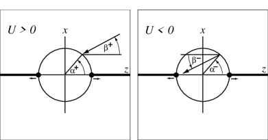
Figure 1: The angle $\alpha$ identifies the point where the particle interacts with the impulse (indicated by a circle) generated by a snapped string localized on the $z$-axis. The angle $\beta$ characterizes the inclination of its trajectory. The superscripts “+” and “–” correspond to the respective values in the (local) Minkowskian coordinate system outside ($U>0$) and the (different) Minkowskian system inside ($U<0$) the impulse.

In the region $U>0$ outside the impulsive wave these parameters are defined as

$$\cot\alpha^{+}={z_{0}/x_{0}}\ ,\qquad\cot\beta^{+}={\dot{z}_{0}/\dot{x}_{0}}\ .$$ (41)

Similarly, behind the impulse in the region $U<0$ we have

$$\cot\alpha^{-}={z_{0}^{-}/x_{0}^{-}}\ ,\qquad\cot\beta^{-}={\dot{z}_{0}^{-}/\dot{x}_{0}^{-}}\ .$$ (42)

Straightforward calculations using (38) give

$$Z_{0}^{1-\delta}=\cot\,({\textstyle\frac{1}{2}}\alpha^{+})\ ,$$ (43)

which implies the relation $\frac{1}{2}(Z_{0}^{1-\delta}-Z_{0}^{\delta-1})=\cot\alpha^{+}$. From (39) and (43) we immediately obtain

$$\cot\alpha^{-} = {\textstyle\frac{1}{2}}(Z_{0}-Z_{0}^{-1})$$ (44)

$$= {\textstyle\frac{1}{2}}[\,\cot^{\,q}\,({\textstyle\frac{1}{2}}\alpha^{+})-\cot^{-q}\,({\textstyle\frac{1}{2}}\alpha^{+})\,]\,,$$

where $q=1/(1-\delta)$. This expression gives the relation $\alpha^{-}(\alpha^{+})$ which identifies the points on both sides of the impulse in the natural Minkowskian coordinate systems.

Analogously we derive the following relation for the velocities,

$$\cot\beta^{-}-\cot\alpha^{-}={\cal N}\,(\cot\beta^{+}-\cot\alpha^{+})\ ,$$ (45)

where

$${\cal N}={\cal N}(\alpha^{+},\beta^{+})=\frac{1-\epsilon}{(1-\delta)(E-D)-(1-\delta)\,2F\cot\beta^{+}}\ .$$ (46)

This is the refraction formula for trajectories of free test particles which cross the spherical impulse.

Notice that the above considerations also apply to geodesics propagating in the privileged directions $\beta^{+}=0$ and $\beta^{+}=\frac{\pi}{2}$. For geodesics parallel to the string, i.e., in the case $\beta^{+}=0$ (implying $\dot{x}_{0}=0$) the right hand side of (45) has to be replaced by the simple expression $(\epsilon-1)/[(1-\delta)2F]$. For trajectories with $\beta^{+}=\frac{\pi}{2}$ which are perpendicular to the strings ($\dot{z}_{0}=0$), the right hand side simplifies to $[(\epsilon-1)\cot\alpha^{+}]/[(1-\delta)(E-D)]$.

Several interesting observations can immediately be done. For $\delta=0$ representing a complete Minkowski space without the impulse and topological defects, one obtains $\alpha^{-}=\alpha^{+}$, ${\cal N}=1$, and consequently $\beta^{-}=\beta^{+}$. There is thus no “shift” and “refraction”, as expected.

For a general $\delta$, it follows from (45) that if $\alpha^{+}=\beta^{+}$ then $\alpha^{-}=\beta^{-}$. This means physically that the radial geodesics (“perpendicular” to the spherical impulse) remain radial also behind the impulse.

Moreover, it can be observed from (46) that the coefficient ${\cal N}$ identically vanishes for spacetimes with the parameter $\epsilon=+1$. Consequently, $\alpha^{-}=\beta^{-}$, which means that the geodesics (24) are refracted by the impulse in such a way that their trajectories become radial. These are thus either exactly focused towards the origin $x=0=z$, or defocused directly from it.

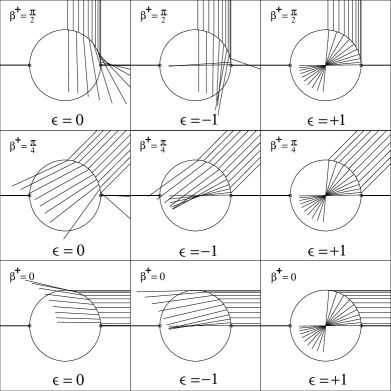
Figure 2: Typical behavior of geodesic trajectories, which are refracted and shifted by the expanding spherical impulse, for various values of $\alpha^{+}$, $\beta^{+}$ and the parameter $\epsilon$. Here $\delta=0.3$.

The typical behavior of geodesics affected by the impulsive gravitational wave (10), (35), as described by the refraction formula (45), is shown in Fig. 2 for various choices of $\alpha^{+},\beta^{+}$, and $\epsilon$. Each test particle follows in the region $U>0$ a trajectory with the inclination angle $\beta^{+}$ until it reaches the spherical impulse at the point represented by $\alpha^{+}$. The impulse influences the particle in such a way that it emerges in the region $U<0$ at the point given by $\alpha^{-}$ and continues to move uniformly along the straight trajectory with inclination $\beta^{-}$. Note that the lines in Fig. 2 represent just the inclination of the geodesic trajectories, not the speed and orientation of the motion — these will be investgated later on.

From Fig. 2 it becomes obvious that the dependence of $\beta^{-}$ on the data $\alpha^{+}$, $\beta^{+}$, and the parameter $\epsilon$ is rather delicate. To shed some light on the details of this dependence we introduce two special “incoming” inclination angles denoted by $\beta^{+}_{\parallel}(\alpha^{+})$ and $\beta^{+}_{\perp}(\alpha^{+})$ defined by the property that the corresponding geodesic behind the impulse are parallel ($\beta^{-}=0$) resp. perpendicular ($\beta^{-}=\pm\frac{\pi}{2}$) to the strings localized along the $z$-axis. It follows immediately from (45) that

$$\cot\beta^{+}_{\parallel} = \frac{E-D}{2F}\ ,$$ (47)

$$\cot\beta^{+}_{\perp} = \frac{(1-\epsilon)\cot\alpha^{+}-(1-\delta)(E-D)\cot\alpha^{-}}{(1-\epsilon)-(1-\delta)\,2F\,\cot\alpha^{-}}\ ,$$

where the functions $D,E,F$ are given by (40), $Z_{0}$ by (43), and $\alpha^{-}$ by (44). The functions (47) are drawn in Fig. 3 for the three types of spacetimes given by $\epsilon=0,-1,+1$, and for a “typical” value of the deficit-angle parameter $\delta=0.3\,$. Both $\beta^{+}_{\parallel}$ and $\beta^{+}_{\perp}$ vanish at $\alpha^{+}=0$. For $\epsilon=0$ the functions $\beta^{+}_{\parallel}(\alpha^{+})<\alpha^{+}<\beta^{+}_{\perp}(\alpha^{+})$ monotonically increase to the values $\cot\beta^{+}_{\parallel}=(1-\delta)/[\delta(1-\frac{1}{2}\delta)]$, $\beta^{+}_{\perp}=\frac{\pi}{2}$ at $\alpha^{+}=\frac{\pi}{2}$. For $\epsilon=-1$ the relation is $\beta^{+}_{\parallel}>\beta^{+}_{\perp}>\alpha^{+}$, and the corresponding values at $\alpha^{+}=\frac{\pi}{2}$ are $\beta^{+}_{\parallel}={\pi}$, $\beta^{+}_{\perp}=\frac{\pi}{2}$. In the case $\epsilon=1$ these two functions coincide for all values of $\alpha^{+}$, which directly follows from (47). The functions grow to a maximum value and then decrease to $\beta^{+}_{\parallel}=\beta^{+}_{\perp}=\frac{\pi}{2}$ at $\alpha^{+}=\frac{\pi}{2}$. The graphs presented in Fig. 3 provide a qualitative picture of the character of the trajectories depending on the choice of the initial angles $\alpha^{+}$, $\beta^{+}$. Trajectories close to $\beta^{+}_{\parallel}(\alpha^{+})$ become “nearly horizontal” behind the impulse, whereas those close to $\beta^{+}_{\perp}(\alpha^{+})$ become “nearly vertical”. Since for $\beta^{+}_{\parallel}$ we have $\dot{x}^{-}_{0}=0$ whereas $\beta^{+}_{\perp}$ implies $\dot{z}^{-}_{0}=0$, it follows that the particles actually stop behind the impulse if we choose $\beta^{+}=\beta^{+}_{\parallel}(=\beta^{+}_{\perp})$ for a given $\alpha^{+}$ in the impulsive spacetime with $\epsilon=+1$.

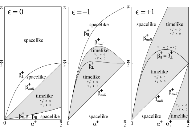
Figure 3: Plots of $\beta^{+}_{\parallel}$, $\beta^{+}_{\perp}$ and $\beta^{+}_{null}\,$, introduced in the text, as functions of the angle $\alpha^{+}$ (again $\delta=0.3$). The causal character of the geodesics with specific initial data is indicated by the shading of the respective regions: grey resp. white corresponds to timelike resp. spacelike geodesics.

Note, however, that the refraction formula (45) while relating the inclination of the trajectories behind the wave to its initial values does not provide any information on the specific speed and orientation of the motion. Of course, the velocity is proportional to the parameters $\dot{x}_{0},\dot{y}_{0},\dot{z}_{0}$, which are the derivatives of space coordinates with respect to the affine parameter $\tau$, see equation (19). However, for physical interpretation of the motion we need the velocity with respect to the Minkowski frame behind the impulse, which is given by

$$(v_{x}^{-},v_{y}^{-},v_{z}^{-})=\left(\frac{\dot{x}_{0}^{-}}{\dot{t}_{0}^{-}},\frac{\dot{y}_{0}^{-}}{\dot{t}_{0}^{-}},\frac{\dot{z}_{0}^{-}}{\dot{t}_{0}^{-}}\right)\ .$$ (48)

From (39) using (41) we obtain

$$v_{x}^{-} =\frac{G}{{{\textstyle\frac{1}{2}}(Z_{0}+Z_{0}^{-1})\,G-(1+\epsilon)(\cot\alpha^{+}-\cot\beta^{+})}}\ ,$$ (49)

$$v_{z}^{-} =\frac{{{\textstyle\frac{1}{2}}(Z_{0}-Z_{0}^{-1})\,G-(1-\epsilon)(\cot\alpha^{+}-\cot\beta^{+})}}{{{\textstyle\frac{1}{2}}(Z_{0}+Z_{0}^{-1})\,G-(1+\epsilon)(\cot\alpha^{+}-\cot\beta^{+})}}\ ,$$

and $v_{y}^{-}=0$, where $G=(1-\delta)[(E-D)-2F\cot\beta^{+}]$. The above expressions determine the velocity of the particle (including its orientation) in the region behind the impulse as a function of the initial parameters $\alpha^{+}$, $\beta^{+}$: The particle moves from the point $\alpha^{-}(\alpha^{+})$ in the refracted direction $\beta^{-}(\alpha^{+},\beta^{+})$ given by (44) (45) in terms of the parameters $\alpha^{+}$, $\beta^{+}$ and its velocity is given by (49).

Each geodesic belonging to the family (24) following the trajectory determined by $\alpha^{+}$, $\beta^{+}$ has a specific causal character. If the magnitude of the velocity is such that $v^{-}\equiv\sqrt{(v_{x}^{-})^{2}+(v_{z}^{-})^{2}}<1$, the geodesic is timelike ($e=-1$). When $v^{-}=1$ it is null ($e=0$), and for $v^{-}>1$ it is spacelike ($e=+1$). Moreover, we can express the condition for the null geodesics explicitly. Substituting from (49) we obtain a quadratic equation for $\cot\beta^{+}$ which can be solved. In the range $\alpha^{+}\in(0,\frac{\pi}{2}]$ there are always two real roots, namely

$$1. \!\!\!\!\beta_{null}^{+}=\alpha^{+}\ ,$$ (50)

$$2. \!\!\!\!\cot\beta_{null}^{+}=\frac{{\epsilon\cot\alpha^{+}-{\textstyle\frac{1}{2}}(Z_{0}^{-1}+\epsilon Z_{0})(1-\delta)(E-D)}}{{\epsilon-{\textstyle\frac{1}{2}}(Z_{0}^{-1}+\epsilon Z_{0})(1-\delta)\,2F}}\ .$$

The first equation in (50) implies that all geodesics of the family (24) which move radially “outside” the impulse are null. In fact, it follows from (38) and (41) that $\dot{U}_{0}=0$, i.e., $U\equiv 0$. These are exactly those null geodesics which generate the spherical impulse itself. Non-trivial null geodesics which cross the impulsive wave are thus given by the second root in (50). Fig. 3 shows the functions $\beta_{null}^{+}(\alpha^{+})$ for the three spacetimes characterized by $\epsilon=0$, $\epsilon=-1$, and $\epsilon=+1$ respectively.

For $\epsilon=0$ it follows immediately from (50) and (47) that $\beta_{null}^{+}=\beta_{\parallel}^{+}$. Therefore, these null geodesics are refracted to rays which are parallel to the strings behind the impulse ($v_{x}^{-}=0,v_{z}^{-}=1$). All geodesics with trajectories given by $\alpha^{+}$, $\beta^{+}$ such that $\beta^{+}_{\parallel}<\beta^{+}<\alpha^{+}$ are timelike with $v_{x}^{-}>0,v_{z}^{-}>0$. All other geodesics are spacelike.

In the case $\epsilon=-1$ it can be shown that the non-trivial root $\beta^{+}_{null}$ in (50) satisfies the relation $\beta^{+}_{\parallel}>\beta^{+}_{null}>\beta^{+}_{\perp}>\alpha^{+}$, as shown in Fig. 3. Again, in the region $\beta^{+}\in(\alpha^{+},\beta^{+}_{null}(\alpha^{+}))$ all the geodesics are timelike with $v_{x}^{-}>0$. At $\beta^{+}_{\perp}$ the velocity $v_{z}^{-}$ changes sign: for $\beta^{+}<\beta^{+}_{\perp}$ we have $v_{z}^{-}>0$, and for $\beta^{+}>\beta^{+}_{\perp}$ we obtain $v_{z}^{-}<0$.

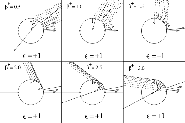
Figure 4: In the region $U<0$ behind the expanding spherical impulse with $\epsilon=+1$, the motion of test particles is always radial, i.e., exactly (de)focusing. Incoming trajectories for various $\beta^{+}$ and $\alpha^{+}$ in the region $U>0$, with the deficit angle parameter $\delta=0.3$, are indicated by dashed lines. The velocity vectors behind the wave are indicated by arrows of the corresponding length and orientation (tachyons are denoted by double arrows).

Finally, the most interesting case is $\epsilon=+1$. In this case the graph shown in Fig. 3 is even more delicate. For a particular value $\alpha^{+}_{c}$ given by the condition $\cot(\frac{1}{2}\alpha^{+}_{c})=(\Delta+\sqrt{\Delta^{2}-1})^{1-\delta}$, where $\Delta^{-2}=2\delta(1-\frac{1}{2}\delta)$, the denominator on the right hand side of (50) vanishes. Therefore, the value of $\beta^{+}_{null}$ jumps at $\alpha^{+}_{c}$ from $\beta^{+}_{null}(\alpha^{+}_{c-})=\pi$ to $\beta^{+}_{null}(\alpha^{+}_{c+})=0$. (Note that $\alpha^{+}_{c}$ monotonically increases from $0$ to $\frac{\pi}{2}$ as the string parameter $\delta$ grows from the value $0$ to $1$.) Consequently, there are two disconnected regions of timelike geodesics. In the “upper” region ($\alpha^{+}<\beta^{+}<\beta^{+}_{null}$) lies the line $\beta^{+}_{\parallel}=\beta^{+}_{\perp}$: particles moving along timelike geodesics with the “incoming position” $\alpha^{+}$ and a suitable “inclination” $\beta^{+}=\beta^{+}_{\parallel}(\alpha^{+})=\beta^{+}_{\perp}(\alpha^{+})$ will exactly stop at the point $x_{0}^{-},z_{0}^{-}$ in the region behind the impulse ($v_{x}^{-}=0=v_{z}^{-}$), see (49). Particles below this boundary ($\beta^{+}<\beta^{+}_{\parallel}=\beta^{+}_{\perp}$) move radially outward since $v_{x}^{-}>0,v_{z}^{-}>0$. On the other hand, timelike particles with $\beta^{+}>\beta^{+}_{\parallel}=\beta^{+}_{\perp}$ for a given $\alpha^{+}$ have $v_{x}^{-}<0,v_{z}^{-}<0$ so that these radially approach the origin. Thus there is an exact focusing effect of the impulse on these timelike geodesics. The same is true for all timelike geodesics in the “lower region” corresponding to initial values $\alpha^{+}$ close to $\frac{\pi}{2}$ and small $\beta^{+}$ (see Fig. 3). The time $t^{-}_{f}=2x_{0}(\cot\alpha^{+}-\cot\beta^{+})/(E-D-2F\cot\beta^{+})$ when each individual particle in the spacetime $\epsilon=+1$ reaches the origin, depends on the particular initial data. These geodesics are explicitly drawn in Fig. 4 with arrows indicating the precise value of the particle velocity behind the impulsive wave. Double arrows correspond to tachyons moving along spacelike geodesics. Notice that for large values of $\beta^{+}$ and small $\alpha^{+}$ some of the incoming trajectories (dashed lines) are drawn inside the circle which indicates the impulse. However, this is not a contradiction as the figure represents just a snapshot at a given time. In fact, the corresponding timelike particles move in the outer region $U>0$ until they are hit by the expanding impulse (which at previous instants of time is a smaller circle). The tachyons move ”acausally” and thus their motion is neither intuitive nor represents the motion of a test particle; this case is included for the sake of completeness.

All the above results can equivalently be obtained also by the “inverse approach”, i.e., starting with the initial data (28) behind the impulse (in the region $U<0$) and evolving these “backward” in time into $U>0$. The solution is given by (29) which has to be substituted into (25). Let us demonstrate this method by considering a simple yet important particular example. Consider a geodesic motion of timelike particles which are at rest behind the impulse generated by a snapping cosmic string, $\dot{x}_{0}=\dot{y}_{0}=\dot{z}_{0}=0$ (so that $\gamma=1$). In other words, we investigate motion of those particles which are exactly stopped by the impulse. Again, we can without loss of generality assume that $y_{0}=0$. Then the constraint (30) implies $\epsilon=+1$ so that such a situation may occur only in the spacetime with this value of the parameter $\epsilon$. Relations (29) then immediately yield

$$Z_{0}=\frac{x_{0}}{\tau_{i}-z_{0}},\ V_{0}=\sqrt{2}\tau_{i},\ \dot{V}_{0}=0,\ \dot{U}_{0}=-\frac{1}{\sqrt{2}}\ .$$ (51)

The motion of the particles in front of the wave is thus given by (25) with the parameters substituted from (51) and (37). We obtain

$$x^{+}_{0}+\,\hbox{i}\,y^{+}_{0}=2\tau_{i}C\ ,\quad\dot{x}^{+}_{0}+\,\hbox{i}\,\dot{y}^{+}_{0}=F\ ,$$

$$z^{+}_{0}=\tau_{i}(B-A)\ ,\quad\ \dot{z}^{+}_{0}={\textstyle\frac{1}{2}}(E-D)\ ,$$ (52)

$$t^{+}_{0}=\tau_{i}(B+A)\ ,\quad\ \ \dot{t}^{+}_{0}={\textstyle\frac{1}{2}}(E+D)\ .$$

As expected, $y^{+}_{0}=0=\dot{y}^{+}_{0}$ since the coefficients $C$ and $F$ are real. From the remaining relations we easily derive (using the definitions (47) and the fact that $\epsilon=+1$)

$$\cot\alpha^{+}\equiv\frac{z^{+}_{0}}{x^{+}_{0}}=\frac{B-A}{2C}={\textstyle\frac{1}{2}}(Z_{0}^{1-\delta}-Z_{0}^{\delta-1})\ ,$$

$$\cot\beta^{+}\equiv\frac{\dot{z}^{+}_{0}}{\dot{x}^{+}_{0}}=\frac{E-D}{2F}\equiv\cot\beta_{\parallel}\equiv\cot\beta_{\perp}\ .$$ (53)

Of course, these results are identical to those obtained previously using the “direct” approach. However, now we know explicitly how to choose the initial data $\alpha^{+}$, $\beta^{+}$ to put the particle at rest behind the impulse at time $\tau_{i}$ in the specific point $x_{0}$, $z_{0}$. For this, one simply substitutes $Z_{0}=x_{0}/(\tau_{i}-z_{0})$ into (53).

IV.2 General $C^{1}$-geodesics

Let us recall again that all the geodesics in the spacetime (10) with the impulsive gravitational wave generated by a snapping cosmic string (35) which we have investigated so far, are very special, i.e., $Z=Z_{0}=$const. (cf. (24)). They are geometrically preferred since they are restricted to a single plane (taken above as $y=0$) which also contains the snapping string localized along the $z$-axis. This fact immediately follows from the constraint (30). Therefore, the corresponding particles move — although not necessarily parallel — “along” the strings. To investigate more general geodesics which “bypass” the strings, we have to relax the condition $Z=Z_{0}$. However, these general geodesics with $\dot{Z}_{0}\not=0$ cannot be found easily in the continuous form of the metric (10). Nevertheless, in (32)-(34) we presented an explicit form of general geodesics which was derived under the assumption that these are $C^{1}$ in the continuous coordinate system (10).

As an interesting particular example, which can be investigated using these expressions, let us now consider geodesics in the $z=0$ plane only. This is the plane of symmetry perpendicular to the strings. We assume that $z_{0}=0=\dot{z}_{0}$ in the region $U<0$ behind the wave. With this, the relations (33) simplify to

$$Z_{i}=\frac{x_{0}+\,\hbox{i}\,y_{0}}{\gamma\tau_{i}}\ ,\qquad\quad V_{i}={\textstyle\frac{1}{\sqrt{2}}}\,(1+\epsilon)\gamma\tau_{i}\ ,$$

$$\dot{Z}_{i}=\frac{\dot{x}_{0}+\,\hbox{i}\,\dot{y}_{0}}{\gamma\tau_{i}}$$

$$\hskip 25.60747pt-(x_{0}+\,\hbox{i}\,y_{0})\frac{(1-\epsilon)\gamma^{2}\tau_{i}+2\epsilon(x_{0}\dot{x}_{0}+y_{0}\dot{y}_{0})}{(1+\epsilon)(\gamma\tau_{i})^{3}}\ ,$$

$$\dot{V}_{i}=\frac{(1-\epsilon)^{2}\gamma^{2}\tau_{i}+4\epsilon(x_{0}\dot{x}_{0}+y_{0}\dot{y}_{0})}{\sqrt{2}(1+\epsilon)\gamma\tau_{i}}\ ,$$

$$\dot{U}_{i}={\textstyle{\sqrt{2}}}\,\,\frac{x_{0}\dot{x}_{0}+y_{0}\dot{y}_{0}-\gamma^{2}\tau_{i}}{(1+\epsilon)\gamma\tau_{i}}\ ,$$ (54)

from which follows that $|Z_{i}|=1$. Therefore the coefficients (36) entering (34) take the following form

$$A=B=\frac{1}{(1-\delta)(1+\epsilon)}\ ,\ C=\frac{Z_{i}^{1-\delta}}{(1-\delta)(1+\epsilon)}\ ,$$

$$D=\frac{(\textstyle{\frac{1}{2}\delta})^{2}+\epsilon(\textstyle{1-\frac{1}{2}\delta})^{2}}{1-\delta}\ ,\ E=\frac{(\textstyle{1-\frac{1}{2}\delta})^{2}+\epsilon(\textstyle{\frac{1}{2}\delta})^{2}}{1-\delta}\ ,$$

$$F=\frac{Z_{i}^{1-\delta}\textstyle{\frac{1}{2}\delta(1-\frac{1}{2}\delta)(1+\epsilon)}}{1-\delta}\ ,$$ (55)

$$A_{,Z}=\frac{\textstyle{\frac{1}{2}\delta}-\epsilon(\textstyle{1-\frac{1}{2}\delta})}{(1-\delta)(1+\epsilon)^{2}Z_{i}}\ ,\ B_{,Z}=\frac{(\textstyle{1-\frac{1}{2}\delta})-\epsilon\textstyle{\frac{1}{2}\delta}}{(1-\delta)(1+\epsilon)^{2}Z_{i}}\ ,$$

$$C_{,Z}=\left(\frac{\bar{Z}_{i}}{Z_{i}}\right)^{\delta/2}\frac{(\textstyle{1-\frac{1}{2}\delta})-\epsilon\textstyle{\frac{1}{2}\delta}}{(1-\delta)(1+\epsilon)^{2}}\ ,$$

$$C_{,\bar{Z}}=\left(\frac{\bar{Z}_{i}}{Z_{i}}\right)^{\delta/2-1}\frac{\textstyle{\frac{1}{2}\delta}-\epsilon(\textstyle{1-\frac{1}{2}\delta})}{(1-\delta)(1+\epsilon)^{2}}\ .$$

Substituting (54), (55) into (34) we obtain an explicit solution which describes the behavior in the region $U>0$ outside the impulse. In particular, we easily derive that

$$z^{+}_{0}\equiv{\textstyle\frac{1}{\sqrt{2}}}({\cal U}_{0}^{+}-{\cal V}_{0}^{+})=0\ ,$$

$$\dot{z}^{+}_{0}\equiv{\textstyle\frac{1}{\sqrt{2}}}(\dot{\cal U}_{0}^{+}-\dot{\cal V}_{0}^{+})=0\ .$$ (56)

Therefore, the geodesics remain in the plane $z=0$ also in the outside region, as is expected from the symmetry of the spacetime. Straightforward but somewhat lengthy calculations for $\eta^{+}_{0}\equiv\frac{1}{\sqrt{2}}(x^{+}_{0}+\,\hbox{i}\,y^{+}_{0})$, $\dot{\eta}^{+}_{0}\equiv\frac{1}{\sqrt{2}}(\dot{x}^{+}_{0}+\,\hbox{i}\,\dot{y}^{+}_{0})$ yield

$$x^{+}_{0}+\,\hbox{i}\,y^{+}_{0}=\frac{(\gamma\tau_{i})^{\delta}}{1-\delta}\,(x_{0}+\,\hbox{i}\,y_{0})^{1-\delta}\ ,$$ (57)

$$\dot{x}^{+}_{0}+\,\hbox{i}\,\dot{y}^{+}_{0}=\left(\frac{x_{0}-\,\hbox{i}\,y_{0}}{x_{0}+\,\hbox{i}\,y_{0}}\right)^{\delta/2}$$

$$\hskip 39.83385pt\times\,\Big{[}(\dot{x}_{0}+\,\hbox{i}\,\dot{y}_{0})-{\cal P}(x_{0}+\,\hbox{i}\,y_{0})\Big{]}\ ,$$ (58)

where

$${\cal P}=-\frac{\delta}{1-\delta}\left(\frac{{\textstyle\frac{1}{2}}\delta(x_{0}\dot{x}_{0}+y_{0}\dot{y}_{0})}{x_{0}^{2}+y_{0}^{2}}+\frac{1-{\textstyle\frac{1}{2}\delta}}{\tau_{i}}\right)\ ,$$ (59)

and $\tau_{i}=\sqrt{(x_{0}^{2}+y_{0}^{2})/(\dot{x}_{0}^{2}+\dot{y}_{0}^{2}-e)}$. The equations (57) and (58) describe the identification of points on the impulse, and the refraction formula in the transverse plane $z=0$, respectively. These admit a natural geometrical interpretation. If we introduce a “polar” representation of positions and velocities by $x_{0}+\,\hbox{i}\,y_{0}\equiv\rho_{0}\exp(\hbox{i}\phi_{0})$, $\dot{x}_{0}+\,\hbox{i}\,\dot{y}_{0}\equiv\dot{\rho}_{0}\exp(\hbox{i}\dot{\phi}_{0})$, we can conclude from (57) that $\phi_{0}^{+}=(1-\delta)\phi_{0}$. As the range of $\phi_{0}$ inside (behind) the spherical impulse spans the whole Minkowski space, $\phi_{0}\in[0,2\pi)$, the range of the angular parameter $\phi^{+}_{0}$ outside is $[0,2\pi(1-\delta))$. Therefore, there is a deficit angle $2\pi\delta$ in front the impulse corresponding to the presence of the (snapped) cosmic string. This is in full agreement with the geometrical construction of the spacetime presented e.g., in PodGri00 . The relation (58) is the refraction formula for geodesics in the symmetry plane $z=0$ perpendicular to the strings. Interestingly, here the effect is totally independent of the parameter $\epsilon$, i.e., the differences between the spacetimes characterized by $\epsilon=0,-1,+1$ disappear in this plane of symmetry. Of course, for $\delta=0$ we obtain a trivial solution $\dot{y}^{+}_{0}=\dot{y}_{0}$, $\dot{x}^{+}_{0}=\dot{x}_{0}$ in the complete Minkowski space without string and impulse. Note also that the factor

$$\left(\frac{x_{0}-\,\hbox{i}\,y_{0}}{x_{0}+\,\hbox{i}\,y_{0}}\right)^{\delta/2}\equiv\>\exp(-\hbox{i}\delta\phi_{0})$$ (60)

in (58) is just an appropriate “rectifying”complex unit factor which ensures the one-to-one correspondence between the identified points on both sides of the impulse (analogously to the function $\alpha^{-}(\alpha^{+})$ given by (44) for longitudinal motion). This can be seen easily if we consider two infinitesimally close parallel null geodesics $y_{0}=0=\dot{y}_{0}$ in the Minkowski region $U<0$ without topological defects. The first geodesic is given by $\phi_{0}=0$, the second one by an angle $\phi_{0}$ near $2\pi$. However, from the formula (58), which reads $\dot{\rho}^{+}_{0}\exp(\hbox{i}\dot{\phi}^{+}_{0})={\cal F}\exp(-\hbox{i}\delta\phi_{0})$, where ${\cal F}$ is a real factor, it follows that $\dot{\phi}^{+}_{0}=-\delta\phi_{0}$. Therefore, outside the impulse the two geodesics which remain parallel are described by $\dot{\phi}^{+}_{0}=0$ and $\dot{\phi}^{+}_{0}$ near to $-2\pi\delta$, respectively. The difference $2\pi\delta$ exactly corresponds to the deficit angle in the (locally) flat space with the string outside the spherical impulse. Therefore, the “pure” physical refraction effect of the impulse on geodesics is described just by the expression in the square bracket on the right hand side of the equation (58).

The above relations can easily be applied to investigate the effect of the impulsive wave on a ring of free test particles. Let us consider a ring in the $z=0$ plane, centered around $x=0=y$, consisting of particles which are at rest in front of the wave, $\dot{x}^{+}_{0}=0=\dot{y}^{+}_{0}$, in the (locally) flat Minkowski region $U>0$. All the particles are simultaneously hit by the impulse at the instant $\tau_{i}$ and the ring starts to deform according to (57), (58). Obviously, it follows from (58) that the velocities of the particles $\dot{x}_{0}$, $\dot{y}_{0}$ behind the impulse ($U<0$) are given by

$$\dot{x}_{0}={\cal P}\,x_{0}\ ,\quad\dot{y}_{0}={\cal P}\,y_{0}\ ,$$ (61)

with ${\cal P}$ given by (59) and $\tau_{i}^{-1}=\sqrt{{\cal P}^{2}+(x_{0}^{2}+y_{0}^{2})^{-1}}$. This yields a self-consistent solution only if

$${\cal P}=-\frac{\delta(1-{\textstyle\frac{1}{2}\delta})}{(1-\delta)\sqrt{x_{0}^{2}+y_{0}^{2}}}\ .$$ (62)

Thus, all the particles of the ring move radially towards the origin in the $z=0$ plane, with the same velocity $v\equiv\sqrt{\dot{x}_{0}^{2}+\dot{y}_{0}^{2}}=\delta(1-{\textstyle\frac{1}{2}\delta})/(1-\delta)$. The ring is deformed by the impulse into contracting and concentric circles. Of course, this is in accordance with the axial symmetry of the spacetime.

A more general situation in which the impulse deforms a sphere of test particles (around the origin) initially at rest is, however, more difficult to investigate explicitly. We can again employ the coordinate freedom $Z\to Z\,\exp(\hbox{i}\phi)$ related to the axial symmetry of the spacetime which corresponds to a simple rotation of the $(x,y)$-planes around the $z$-axis. Using (36) and (34) we conclude $\eta_{0}^{+}\to\eta_{0}^{+}\,\exp[\hbox{i}(1-\delta)\phi]$, $\dot{\eta}_{0}^{+}\to\dot{\eta}_{0}^{+}\,\exp[\hbox{i}(1-\delta)\phi]$. Therefore, without loss of generality we can always set for each individual test particle $\eta_{0}^{+}$ to be real, i.e., $y_{0}^{+}=0$. Moreover, we are considering the motion of test particles which are at rest outside the expanding impulsive wave, $\dot{\eta}_{0}^{+}=0$, $\dot{z}_{0}^{+}=0$. From (34), (36) and (33) it then follows that $Z_{i}$ and $\dot{Z}_{i}$ are real so that $y_{0}=0=\dot{y}_{0}$. The sphere of test particles is thus deformed into an axially symmetric surface which is fully described by the section $y=0$.

Setting $y_{0}=0=\dot{y}_{0}$ in (33) we can now simplify $\dot{Z}_{i}$ to

$$\dot{Z}_{i}=$$ (63)

$$\ \frac{[(1-\epsilon)\gamma\tau_{i}-(1+\epsilon)z_{0}]\dot{x}_{0}-[(1-\epsilon)\gamma-(1+\epsilon)\dot{z}_{0}]x_{0}}{(\gamma\tau_{i}-z_{0})[(1+\epsilon)\gamma\tau_{i}-(1-\epsilon)z_{0}]}\ .$$

Consequently, for these geodesics $\dot{Z}_{i}=0$ if and only if the constraint (30) is satisfied. In such a case, the geodesics reduce to the privileged family (24) for which $Z_{i}=Z_{0}=\,$const. which we investigated in detail above. However, these special geodesics exclude observers which are static in the Minkowski region outside the impulse. Indeed, from the conditions $\dot{x}_{0}^{+}=0=\dot{z}_{0}^{+}$ we obtain using (34) the relation $(A-B)F=(D-E)C$. Substituting from (37) this reduces to $Z_{0}^{\delta-1}(\frac{1}{2}\delta p-\epsilon Z_{0}^{2})=Z_{0}^{1-\delta}(\frac{1}{2}\delta p-1)$, which has no solution except for observers in the plane $z=0$ in spacetime with $\epsilon=+1$, which we investigated in (61), (62).

Therefore, to obtain a nontrivial family of geodesics corresponding to initially static test particles, one has to consider the more complicated situation in which $\dot{Z}_{i}\not=0$. It is difficult to obtain the description of these geodesics in an explicit form. Nevertheless one can immediately argue that the motion can not be spherically symmetric. For example, for the case $\epsilon=+1$ we observe from (63) that $z_{0}\dot{x}_{0}\not=x_{0}\dot{z}_{0}$ which, in terms of (42), can be expressed as $\alpha^{-}\not=\beta^{-}$. Obviously, the trajectories of such geodesics behind the impulse are not radial, i.e., these do not “point” towards the origin. A sphere of free test particles which are at rest in the Minkowski region outside the expanding impulsive wave is thus not deformed into spherical shapes, but to a more complicated (axially symmetric) surface.

V Concluding remarks

We presented a complete solution of geodesic motion — although not always in closed explit form — which describes the effect on free particles of expanding spherical impulsive gravitational waves propagating in a flat background. In particular, we discussed in detail the geodesics in the axially symmetric spacetimes with the impulse generated by a snapping cosmic string. The above results can be used not only for physical interpretation of the behavior of free test particles but also as a starting point for a mathematically rigorous distributional treatment of impulsive Robinson–Trautman spacetimes. To be more specific, the geodesics of the special family (24) provide the key to understand the discontinuous transformation relating the distributional and the continuous form or the metric (analogous to the case of impulsive pp-waves; cf. KunSt99 ). These interesting questions will, however, be investigated elsewhere.

- (1) R. Penrose, in General Relativity, edited by L. O’Raifeartaigh (Clarendon, Oxford, 1972).
- (2) Y. Nutku and R. Penrose, Twistor Newsletter, No. 34, 11 May, 9 (1992).
- (3) P. A. Hogan, Phys. Rev. Lett. 70, 117 (1993).
- (4) P. A. Hogan, Phys. Rev. D49, 6521 (1994).
- (5) J. Podolský and J. B. Griffiths, Class. Quantum Grav. 16, 2937 (1999).
- (6) J. B. Griffiths, J. Podolský and P. Docherty, Class. Quantum Grav. 19, 4649 (2002).
- (7) D. Kramer, H. Stephani, M. A. H. MacCallum and E. Herlt, Exact Solutions of Einstein’s Field Equations (Cambridge University Press, Cambridge, 1980).
- (8) R. Steinbauer, J. Math. Phys. 39, 2201 (1998).
- (9) M. Kunzinger and R. Steinbauer, Class. Quantum Grav. 16, 1255 (1999).
- (10) J. F. Colombeau, New Generalized Functions and Multiplication of Distributions (North Holland, Amsterdam, 1984).
- (11) J. F. Colombeau, Multiplication of Distributions (Springer, Berlin, 1992).
- (12) R. Gleiser and J. Pullin, Class. Quantum Grav. 6, L141 (1989).
- (13) J. Bičák, Astron. Nachr. 311, 189 (1990).
- (14) J. Bičák and B. Schmidt, Class. Quantum Grav. 6, 1547 (1989).
- (15) J. Podolský and J. B. Griffiths, Gen. Relativ. Gravit. 33, 37 (2001); 33, 59 (2001).
- (16) E. T. Newman and R. Penrose, J. Math. Phys. 3 566 (1962).
- (17) J. Podolský and J. B. Griffiths, Class. Quantum Grav. 17, 1401 (2000).
- (18) A. García Díaz and J. F. Plebański, J. Math. Phys. 22 2655 (1981).
- (19) J. Bičák and J. Podolský, J. Math. Phys. 40 (1999) 4495.
- (20) J. Bičák and V. Pravda, Class. Quantum Grav. 15, 1539 (1998).