Doing numerical cosmology with the Cactus code
Abstract
The article presents some aspects concerning the construction of a new thorn for the Cactus code, a complete 3-dimensional machinery for numerical relativity. This thorn is completely dedicated to numerical simulations in cosmology, that means it can provide evolutions of different cosmological models, mainly based on Friedman-Robertson-Walker metric. Some numerical results are presented, testing the convergence, stability and the applicability of the code.
1 Introduction
The core of modern cosmology is the theory of General Relativity, ([1]-[2]), a 4-dimensional theory involving one dimension of time and three of space, having as field equations the Einstein equations :
| (1) |
where is the cosmological constant, the Ricci tensor, the Ricci scalar, the space-time metric, the stress-energy tensor, G the gravitational constant, the speed of light and . Numerical Relativity (NR) is concerned with the study of numerical solutions of the Einstein’s equations for the gravitational field ([4]), and when we apply these equations to cosmological models we have numerical cosmology as a branch of NR. Einstein equations are an extremely complicated system of coupled, non-linear, partial differential equations and solving them numerically makes enormous demands on the processing power and memory of a computer. The Cactus code ([5]) has been mainly designed as a computational toolkit (freely available for the scientific community) for simulating different systems of partial differential equations, as Einstein equations are The code can be used to simulate fully 3-dimensional systems with strong gravitational fields: collapsing gravitational waves, colliding black-holes, neutron stars, and other violent astrophysical processes generating gravitational waves.
As a branch of NR, numerical cosmology can use the Cactus code for his purposes. Although Einstein field equations reduce to a small number of equations in most cosmological models ([7]-[8]), trying to simulate more complex models (as models with cosmological constant or having matter fields coupled with gravity) it becomes difficult to compose special numerical codes for every specific case. Thus our purpose was to develop a piece of code to be used inside a general numerical machinery for solving Einstein equations, as the Cactus code is. This article is a report on how we extended the Cactus code for numerical cosmology. In this purpose we developed a new thorn of the Cactus code (“thorns” are called the computer code packages embedded in Cactus code for some specific application). The starting point of this new thorn, called “Cosmo” was an existent thorn of the Cactus code (the “Exact” thorn) previously reported in ([6]) for testing the Cactus code on exact solutions of the Einstein equations.
We investigated some cosmological models being exact solutions of the Einstein equations in our previous article ([6]). Here the scale factor of the universe () and thus the components of the metric tensor are known analytic function of time, given in the code at the initial time as initial data. But in our new Cosmo thorn, the main point is that we have to use the general Robertson-Walker metric, having the scale factor of the universe () as a unknown function to be evolved during the time evolution of the Einstein equations through the Cactus code. Thus the only job to be done by the Cosmo thorn is to provide good initial data (that means at the initial time considered the actual time of the universe, for example) and then let the Cactus code to solve the Einstein equations through the time. In addition it is necessary to prescribe convenient boundary values for the functions and variables involved. This is necessary because the Cactus code has a limited boundary methods implemented, not appropriate for our numerical cosmology purposes.
The article is organized as follows : the next section 2, presents some general facts about the way we built the Cosmo thorn, how we solved the problems exposed above and the necessary theoretical cosmology background. Section 3 is dedicated to a matter dominated universe model based on Robertson-Walker metric ([7]), with pressure-less matter - “dust” and without cosmological constant. Models with cosmological constant are presented in the next section 4 where we concentrated again only on models having matter as a pressure-less dust. A wide larger class of possible initial data is possible including the so called “coasting cosmologies”, models not having as a starting point a Big Bang. In all cases studied and reported in this article we investigated the convergence and the stability of the Cactus code, in the same way we presented in detail in [6].
As a major conclusion we have to point out the good second order convergent and stable behavior of the code, even in the cases we studied both forward and backward time evolutions. Future perspective are open for developing this thorn for inflationary models. It is in our view to study those models having one or more scalar field coupled with gravity to control the behavior of the model and to simulate an accelerated late time evolution, actually called “cosmic acceleration” being well proved experimentally in the last years. Thus together with other similar thorns being in preparation at AEI, we shall have a new class of applications for the Cactus code, a major instrument for new studies in numerical cosmology and in cosmology, in general.
Being included in the list of thorns of the Cactus code, actually the files for our thorn are available by request, directly at the author’s e-mail address and in the near future it will be included in the CVS repository of the Cactus code (see [5]) for free download.
The simulations were performed mainly on single processor machines, using both the AEI computer network (SGI or Dec machines with UNIX operating system) and a Pentium III machine with a UNIX FreeBSD operating system at the West University of Timişoara. Some of the simulations, with similar results, were also done on the Origin 2000 supercomputer at the AEI.
Through this article and in the Cactus code we shall use geometrical units with .
2 The Cactus code, the Robertson-Walker metric and the Cosmo Thorn
As we mentioned earlier, in modern cosmology we are using the Robertson-Walker metric (RW), namely ([7]-[8])
| (2) |
or in isotropic coordinates :
| (3) |
where
as a generic metric for describing the dynamics of the universe through the Einstein equations (1). Here is a constant with arbitrary value, positive (for closed universes), negative (for open universe) and zero for flat universes. Usually, this constant is taken , or respectively. When we consider all the matter in the universe as a perfect fluid, the stress-energy tensor may be given as
| (4) |
and is necessary to prescribe a state equation, i.e. a relation between the pressure and the density of the universe . For matter dominated universes usually the pressure is and this will be the case we concentrated in our simulations.
As our main purpose was to build a new thorn for the Cactus code, generically named from now one “The Cosmo thorn” for evolving the RW metric above in all three cases for and . The main problem was to to ”convince” Cactus to evolve, without having the time behavior of function (actually, is a function of the thorn). Although we used the same strategy as in the above mentioned Exact thorn (see [6]) here, not having an analytic function of time for the solution was to provide Cactus code all initial data he needs, namely and at the initial time we choose ! As a result, new routines were added for calculating the extrinsic curvature [3] components at the initial time, namely :
| (5) |
where is the Hubble constant function (!). Note that we have here as lapse function, and a shift vector as , as always in RW cosmology.
Another item we concentrated on was the boundary problem : - Cactus code and the thorns which solve numerically the Einstein equations (namely ADM_BSSN and ADM - see [5]) have not implemented proper boundary conditions for the RW metric. In our previous article [6] on Exact thorn we used “flat” boundary condition but this is not appropiate here ! To solve this problem we used a simple hint : and are functions of time only, thus they are constant on the numerical grid at one time, having the same value inside the grid and on the boundary. As a result, we added a new boundary method through a new value of the parameter bound of the ADM_BSSN thorn (see [5] and [6]), called external which activates some new routines we composed in this purpose, having as a generic name recover. In these routines the spatial metric components and the extrinsic curvature components on the boundaries are “recovered” from the values of the and on the interior points by calculating them using equations (2) and (5). Also these new boundary conditions are necessary during the intermediate steps of integration used by ADM_BSSN thorn in the so-called “IterativeCN.F” routine (where a three steps Cranck-Nicholson integration method is applied). For this purpose we slightly modified the “IterativeCN.F” routine for “injecting” our specific “recover” boundary values. Actually this was possible through a facility of the Cactus code which makes possible to call different routines from different thorns using special “include” commands (see [5]).
3 Friedman-Robertson-Walker (FRW) cosmologies
By “FRW cosmologies” we mean those cosmological models based on the above RW metric and being solutions of the Einstein equations (1) without cosmological constant () - see for example ([7]) and ([8]). Restricting ourselves only to matter dominated universes (i.e. ) as we mentioned earlier, and solving the conservation law of the perfect fluid which emulates the matter, we have for the stress-energy tensor components
| (6) |
where is a constant depending on the the mass density of the universe at the initial time . Solving the Einstein equations for this constant and at the initial time where and , we have
| (7) |
where is the deceleration parameter at the initial time, i.e.
| (8) |
and is the so-called density factor, defined as
| (9) |
being the initial density of the universe and the critical density (i.e. the density of a flat three-dimensional universe where ). It is proven ([8]) that we have :
| (10) |
In order to provide initial data for the Cactus code we need to solve the Einstein equations at the initial time for the initial Hubble constant (to calculate the values of the extrinsic curvature through equation (5)) and for the initial scale factor . It is known that we have here three solutions, depending on the geometric factor . Thus, for (flat three-dimensional spacetime) where
we have (see LABEL:8 eq. 4.37)
| (11) |
and we shall take , as a value for calculating, for now one the relative scale factor, i.e. which will be our numerical output. For the case of closed universe, we have
In this case (as in the next one for ) we do not have an analytic solution for the scale factor, but for the initial time we can easily obtain that (LABEL:8 eq. 4.51) :
| (12) |
and the initial scale factor is :
| (13) |
Finally, for the open universes () where we have
As it is shown ([8] eq. 4.64), here we have :
| (14) |
and the initial scale factor is :
| (15) |
With these results reminded, we can now proceed to explain how we produced our simulations. Taking as initial data the initial time () in billion years, being an internal parameter of the Cactus code, namely CCTK_intitial_time, we then have all the variables (in our geometrical units with , of course) rescaled in billion years. We also have the initial value of the deceleration parameter, denoted in the code as robson_q. As output we have the scale factor, more precisely the relative scale factor (denoted in the code as raza ) and the Hubble parameter function H(t) (denoted in the code as hubble. For evolving these two functions we produced two internal routines of the thorn, which mainly calculates their values from the general output values provided by the Cactus code and the ADM_BSSN thorn (as the extrinsic curvature and the three-dimensional metric components).
Here we shall present the results we obtained on evolving a matter dominated universe (i.e pressure-less matter, ) based on the RW metric. Some explanations are necessary in order to clarity our figures ( see also ([6])). Here and in the next figures, “normalized” means the L2 norm of the respective function calculated using all the values of the function on the computational grid at one time and the respective output Cactus files are denoted with _nm2 extension.

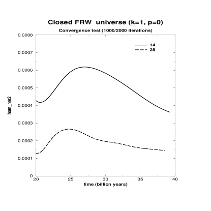
Cactus code is evolving the Einstein equations using the 3+1 decomposition of space-time (both in ADM or BSSN evolution methods -see ([3]) and ([10])). Thus the Einstein equations can be split in two groups : the dynamic equations (for the time derivatives of the three-dimensional metric and extrinsic curvature) and the constraint equations (the Hamiltonian constraint and the Momentum constraint) - see [1] and [3]. The constraint equations are satisfied during all time evolution of the system. Thus one of the main tests on the convergence in the Cactus code is given by the time behavior of the Hamiltonian constraint (an output of the Cactus code through a thorn called ADMConstraints, namely ham). In some of the next figures (here and in the next sections) we show the convergence of the L2 norm of the Hamiltonian constraint for different number of iterations, using two different resolutions on the grid, one with and the second with points (both grids cover the same region of spacetime, so the grid with more points has a smaller value of the finite difference interval ). Notice that the Hamiltonian constraint for a true solution of the Einstein equations should be equal to zero. Finite differencing errors imply that the numerical solution will have a non-vanishing value of the Hamiltonian constraint. For a consistent finite difference approximation of the Einstein equations, we should expect the Hamiltonian constraint to approach zero as the resolution is increased. For a second order approximation, the value of the Hamiltonian constraint should go down by a factor of four when the resolution is doubled. This was the method to test the convergence of the code in all examples presented in this article. We have obtained good second order convergence in all examples as is shown in the next figures.
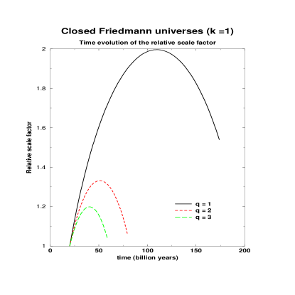
First of our figures (1 and 2) are pointing out the convergence of the code for different examples of FRW cosmologies. The time is scaled in billion years (as for all figures in this section) starting with an initial time of 20 billion years. As it is obvious from these figures a good second order convergence is visible, even for long time evolutions. For the case of the closed universe () we had to restrict our simulations only till around 9000 iterations (for a grid with points) because in this case the universe is evolving to a Big Crunch (opposite to the Big Bang) as it is pointed out in the right panel of the next figure (3). Here the scale factor is evolving to a maximum having the value
twice of the actual value (we used here ). For spatially flat universes we used, of course, and for open universes we had .


Figure (3) contains also in his left panel the evolution of the Hubble parameter function in time. We plotted here, for convenience the modulus of this function being calculated through the L2 norm as is output by the code.


The same comment is valuable for the left panel of the figure (4) where we can point out also the coincidence of the minimum zero value of the Hubble parameter with the maximum of the scale factor from the previous figure (3). The right panel of (4) is dedicated to the simultaneous plot of the three cases, pointing out the differences between the geometries of the three models.


Last of our figures from this section, (5) contains the plots of the relative scale factor time evolution for different closed matter dominated FRW universes, having different deceleration parameter (i.e. different density parameters). It is visible here that as the deceleration parameter (density parameter) is increasing so is decreasing the time-life of the closed universe between a Big-Bang and a Big-Crunch.
4 FRW cosmologies with cosmological constant
Here we shall deal with cosmologies based on the above RW metric but having a non-vanishing cosmological constant. In spite of the failure of the the initial tentative of Einstein to use the cosmological constant as a trick to fit general relativity with, at that time presumed, static universe, the cosmological constant is again used in modern cosmology in order to establish more realistic models of the universe, as the inflationary models and, recently, the so called cosmic acceleration. Early attempts (see ([9])) on using numerical routines for solving the Einstein equations for these models were reported. Because our goal is to implement in the Cactus code a thorn for doing similar simulations, but on a larger scale and fully three-dimensional we shall refer to these previous results only for comparing our results. Meanwhile we shall use here the same notations and scaling of the parameters as in ([9]) for prescribing the initial data sets for the Cactus code.
This time I will proceed in a slightly different way than in the previous section, scaling all our variables and parameters in terms of the initial value of the Hubble parameter function , which is not completely free in our universe, having been measured to within a factor of 2. Thus for the cosmological constant for instance, we use as a basic parameter, denoted in the code with robson_l. Of course, for dimensional scaling reasons we prescribed at the initial time . Thus, for example, at the output we have the relative value of the Hubble function . Meanwhile we need a parameter to describe the density of the universe, and this time we used instead of the deceleration parameter (remark that here we have no more the relation ). We have also the Gaussian curvature defined as
which will be, of course identical to the geometric factor at the initial time when we take the initial scale factor as we done in our simulations. Following the line indicated in ([9]) we can define the density factor as
| (16) |
where is the initial density of the matter in the universe. Now solving the Einstein equations at the initial time and after some algebraic manipulations we obtain (for , ) :
| (17) |
and for the stress-energy tensor (where we included also the term containing the cosmological factor, as we did in ([6])) :
| (18) |
Now our numerical results are pointed out in the next figures. First we show, in figure (6) the time evolution of the scale factor for some cosmological models, having the density factor being (left panel) and (right panel). The models are differentiated by their respective cosmological constant (more precisely the factor ). For the time scale we used here Hubble time units, i.e. the time is expressed as where is the Hubble time : . In these simulations, as in the next ones we started from the actual time (taken here ) and we investigated the time behavior of the model in both directions of time, forward, as well as backward in time.


Next figure (7) shows, in his left panel some special cases of FRW models with cosmological constant, where the scale factor shows off a different evolution : namely it starts somewhere back in time with a certain finite value, it decreases in time, then it has a period (longer or shorter) of constant value, evolving finally as an expanding model (of De-Sitter type, for example). These models, having a period of constant value of the scale factor, are sometimes called “coasting cosmologies” and are investigated as an alternative (realistic or not) to the standard Big-Bang model, not being generated from a Big-Bang, as can be seen from our simulations. The right panel of the figure (7) contains the time evolution of the Hubble constant function (the L2 norm, as it is output by the Cactus code, otherwise the values after the null minimum value being negative ones) for a model with and .


We must point out that we performed here also several convergence tests, as in the previous section, obtaining again good second order convergence. As an example we shall present in the last figure (8) the convergence test for and points on the grid for a model having again and for an evolution forward in time (left panel) and backward in time (right panel).


Acknowledgments
The author is deeply indebted to Prof. E. Seidel for patience, continuous support and encouragement, and to prof. Schutz for his understanding and help. The friendly hospitality and environment the author experienced at AEI during his visits is kindly acknowledged.
References
- [1] Misner C.W., Thorne K.S., Wheeler J.A. : Gravitation, Freeman, San Francisco, (1973)
- [2] d’Inverno R.: Introducing Einsten’s Relativity, Clarendon Press, Oxford, (1992)
- [3] Arnowitt R., Deser S., Misner C.W. : Gravitation - an introduction to current research, ed. by L. Witten, John Wiley and Sons, New York, (1962)
- [4] Hehl F.W., Puntigam R., Ruder H. (eds.) : Relativity and Scientific Computing, Springer Verlag, see the lectures of E. Seidel (p.25), P. Laguna (p. 88) and C. Bona (p. 69) , (1996)
- [5] http://www.cactuscode.org and E. Seidel, Wai-Mo Suen, Journ. Comp. Appl. Math., 109, p. 493, (1999), B. Brügmann, Ann. Phys. (Leipzig), 9, No. 3-5, p. 227 (2000)
- [6] Vulcanov D.N., Alcubierre M, Intern. Journ. of Modern Physics C - Physics and Computers, vol. 13, no. 7, p. 837, (2002)
- [7] J.N. Islam, An Introduction to Mathematical Cosmology, Cambridge University Press, Cambridge, (1992)
- [8] J.V. Narlikar, Introduction to Cosmology, Jones and Brtlett Publishers, Inc. Boston, Portola Valley, (1983)
- [9] J.E. Felten, Reviews of Modern Physics, Vol. 58, No. 3, p. 689, (1986)
- [10] T. W. Baumgarte and S. L. Shapiro, Phys. Rev. D 59, 024007, (1999) and M. Shibata, T. Nakamura, Phys. Rev. D 52, 5428, (1995)