Practical speed meter designs for QND gravitational-wave interferometers

Abstract

In the quest to develop viable designs for third-generation optical interferometric gravitational-wave detectors (e.g., LIGO-III and EURO), one strategy is to monitor the relative momentum or speed of the test-mass mirrors, rather than monitoring their relative position. A previous paper analyzed a straightforward but impractical design for a speed-meter interferometer that accomplishes this. This paper describes some practical variants of speed-meter interferometers. Like the original interferometric speed meter, these designs in principle can beat the gravitational-wave standard quantum limit (SQL) by an arbitrarily large amount, over an arbitrarily wide range of frequencies. These variants essentially consist of a Michelson interferometer plus an extra “sloshing” cavity that sends the signal back into the interferometer with opposite phase shift, thereby cancelling the position information and leaving a net phase shift proportional to the relative velocity. In practice, the sensitivity of these variants will be limited by the maximum light power $W_{\rm circ}$ circulating in the arm cavities that the mirrors can support and by the leakage of vacuum into the optical train at dissipation points. In the absence of dissipation and with squeezed vacuum (power squeeze factor $e^{-2R}\simeq 0.1$) inserted into the output port so as to keep the circulating power down, the SQL can be beat by $h/h_{\rm SQL}\sim\sqrt{W_{\rm circ}^{SQL}e^{-2R}/W_{\rm circ}}$ at all frequencies below some chosen $f_{\rm opt}\simeq 100$ Hz. Here $W_{\rm circ}^{SQL}\simeq 800{\rm kW}(f_{\rm opt}/100{\rm Hz})^{3}$ is the power required to reach the SQL in the absence of squeezing. [However, as the power increases in this expression, the speed meter becomes more narrow band; additional power and re-optimization of some parameters are required to maintain the wide band. See Sec. III B.] Estimates are given of the amount by which vacuum leakage at dissipation points will debilitate this sensitivity (see Fig. 12); these losses are 10% or less over most of the frequency range of interest ($f\gtrsim 10~{}\rm Hz$). The sensitivity can be improved, particularly at high freqencies, by using frequency-dependent homodyne detection, which unfortunately requires two 4-kilometer-long filter cavities (see Fig. 4).

I Introduction

This paper is part of the effort to explore theoretically various ideas for a third-generation interferometric gravitational-wave detector. The goal of such detectors is to beat, by a factor of 5 or more, the standard quantum limit (SQL)—a limit that constrains interferometers [1] such as LIGO-I which have conventional optical topology [2, 3], but does not constrain more sophisticated “quantum nondemolition” (QND) interferometers [4, 5].

The concepts currently being explored for third-generation detectors fall into two categories: external readout and intracavity readout. In interferometer designs with external readout topologies, light exiting the interferometer is monitored for phase shifts, which indicate the motion of the test masses. Examples include conventional interferometers and their variants (such as LIGO-I [2, 3], LIGO-II [6], and those discussed in Ref. [7]), as well as the speed-meter interferometers discussed here and in a previous paper [8]. In intracavity readout topologies, the gravitational-wave force is fed via light pressure onto a tiny internal mass, whose displacement is monitored with a local position transducer. Examples include the optical bar, symphotonic state, and optical lever schemes discussed by Braginsky, Khalili, and Gorodetsky [9, 10, 11]. These intracavity readout interferometers may be able to function at much lower light powers than external readout interferometers of comparable sensitivity because the QND readout is performed via the local position transducer (perhaps microwave-technology based), instead of via the interferometer’s light; however, the designs are not yet fully developed.

At present, the most complete analysis of candidate designs for third-generation external-readout detectors has been carried out by Kimble, Levin, Matsko, Thorne, and Vyatchanin [7] (KLMTV). They examined three potential designs for interferometers that could beat the SQL: a squeezed-input interferometer, which makes use of squeezed vacuum being injected into the dark port; a variational-output scheme in which frequency-dependent homodyne detection was used; and a squeezed-variational interferometer that combines the features of both. (Because the KLMTV designs measure the relative positions of the test masses, we shall refer to them as position meters, particularly when we want to distinguish them from the speed meters that, for example, use variational-output techniques.) Although at least some of the KLMTV position-meter designs have remarkable performance in the lossless limit, all of them are highly susceptible to losses.

In addition, we note that the KLMTV position meters each require four kilometer-scale cavities (two arm cavities + two filter cavities). The speed meters described in this paper require at least three kilometer-scale cavities [two arm cavities + one “sloshing” cavity (described below)]. If we use a variational-output technique, as KLMTV did, the resulting interferometer will have five kilometer-scale cavities (two arm cavities + one sloshing cavity + two filter cavities). This is shown in Fig. 4 below.

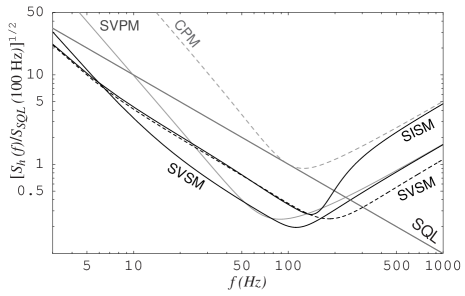
FIG. 1.: Comparison of noise curves (with losses) of several interferometer configurations. Each of these curves has been optimized in a way that is meant to illustrate their relative advantages and disadvantages. The conventional position meter (CPM) [7] has $W_{\rm circ}=820~{}\rm kW$ and bandwidth $\gamma=cT/4L=2\pi\times 100~{}\rm Hz$. The squeezed-input speed meter (SISM)—optmized to agree with the conventional position meter at high frequencies—has power squeeze factor $e^{-2R}=0.1$, optimal frequency $\omega_{\rm opt}=2\pi\times 105~{}\rm Hz$, extraction rate $\delta=2\omega_{\rm opt}$, and sloshing frequency $\Omega=\sqrt{3}\omega_{\rm opt}$. The squeezed-variational position meter (SVPM) [7] has the same parameters as the conventional position meter, with power squeeze factor $e^{-2R}=0.1$. There are two squeezed-variational speed-meter curves (SVSM). One (black dashes) uses the same parameters as the squeezed-input speed meter. The other (solid curve) has been optimized to compare more directly with the squeezed-variational position meter; it has $\Omega=2\pi\times 95~{}\rm Hz$ and $\delta=2\pi\times 100~{}\rm Hz$ (note that our $\delta$ is equivalent to the bandwidth $\gamma$ used to describe the interferometers in Ref. [7]).

The speed meter described in this paper can achieve a performance significantly better than a conventional position meter, as shown in Fig. 1. (By “conventional,” we mean “without any QND techniques.” An example is LIGO-I.) The squeezed-input speed meter (SISM) noise curve shown in that Fig. 1 beats the SQL by a factor of $\sqrt{10}$ in amplitude and has fixed-angle squeezed vacuum injected into the dark port [this allows the interferometer to operate at a lower circulating power than would otherwise be necessary to achieve that level of sensitivity, as described by Eq. (3) below]. The squeezed-variational position meter (SVPM), which requires frequency-dependent squeezed vacuum and homodyne detection, is more sensitive than the squeezed-input speed meter over much of the frequency range of interest, but the speed meter has the advantage at low frequencies. It should also be noted that the squeezed-variational position meter requires four kilometer-scale cavities (as described in the previous paragraph), whereas the squeezed-input speed meter requires three.

If frequency-dependent homodyne detection is added to the squeezed-input speed meter, the resulting squeezed-variational speed meter (SVSM) can be optimized to beat the squeezed-variational position meter over the entire frequency range. Figure 1 contains two squeezed-variational speed meter curves; one is optimized to match the squeezed-input speed meter curve at low frequencies, and the other is optimized for comparison with the squeezed-variational postion-meter curve (resulting in less sensitivity at high frequencies).

The original idea for a speed meter, as a device for measuring the momentum of a single test mass, was conceived by Braginsky and Khalili [12] and was further developed by Braginsky, Gorodetsky, Khalili, and Thorne [13] (BGKT). In their appendix, BGKT sketched a design for an interferometric gravity wave speed meter and speculated that it would be able to beat the SQL. This was verified in Ref. [8] (Paper I), where it was demonstrated that such a device could in principle beat the SQL by an arbitrary amount over a wide range of frequencies. However, the design presented in that paper, which we shall call the two-cavity speed-meter design, had three significant problems: it required (i) a high circulating power ($\sim$ 8 MW to beat the SQL by a factor of 10 in noise power at 100 Hz and below), (ii) a large amount of power coming out of the interferometer with the signal ($\sim$ 0.5 MW), and (iii) an exorbitantly high input laser power ($\gtrsim$ 300 MW). The present paper describes an alternate class of speed meters that effectively eliminate the latter two problems, and techniques for reducing the needed circulating power are discussed. These improvements bring interferometric speed meters into the realm of practicality.

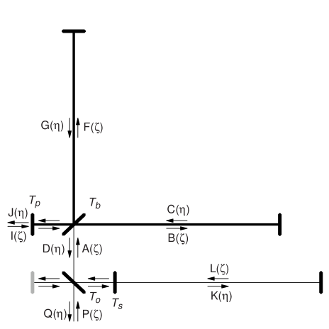
FIG. 2.: Simple version of three-cavity design for speed-meter interferometer. The main laser input port is denoted by $I(\zeta)$, where $\zeta=t-z/c$. The signal is extracted at the bottom mirror [denoted $Q(\eta)$, where $\eta=t+z/c$]. The difference between the one- and two-port versions is the mirror shown in gray.

A simple version of the three-cavity speed-meter design to be discussed in this paper is shown in Fig. 2. In (an idealized theorist’s version of) this speed meter, the input laser light [with electric field denoted $I(\zeta)$ in Fig. 2] passes through a power-recycling mirror into a standard Michelson interferometer. The relative phase shifts of the two arms are adjusted so that all of the input light returns to the input port, leaving the other port dark [i.e., the interferometer is operating in the symmetric mode so $D(\eta)=0$ in Fig. 2]. In effect, we have a resonant cavity shaped like $\perp$. When the end mirrors move, they will put a phase shift on the light, causing some light to enter the antisymmetric mode (shaped like $\vdash$) and come out the dark port. So far, this is the same as conventional interferometer designs (but without the optical cavities in the two interferometer arms).

Next, we feed the light coming out of the dark port [$D(\eta)$] into a sloshing cavity [labeled $K(\eta)$ and $L(\zeta)$ in Fig. 2]. The light carrying the position information sloshes back into the “antisymmetric cavity” with a phase shift of $180^{\circ}$, cancelling the position information in that cavity and leaving only a phase shift proportional to the relative velocity of the test masses. The sloshing frequency is

$$\Omega=\frac{c\sqrt{T_{\rm s}}}{2L}\,,$$ (1)

where $T_{\rm s}$ is the power transmissivity of the sloshing mirror, $L$ is the common length of all three cavities, and $c$ is the speed of light. We read the velocity signal [$Q(\eta)$] out at a extraction mirror (with transmissivity $T_{\rm o}$), which gives a signal-light extraction rate of

$$\delta=\frac{cT_{\rm o}}{L}\,.$$ (2)

We have used the extraction mirror to put the sloshing cavity parallel to one of the arms of the Michelson part of the interferometer, allowing this interferometer to fit into the existing LIGO facilities. The presence of the extraction mirror essentially opens two ports to our system. We can use both outputs, or we can add an additional mirror to close one port (the gray mirror in Fig. 2). We will focus on the latter case in this paper.

The sensitivity $h$ of this interferometer, compared to the SQL, can be expressed as

$$\frac{h}{h_{SQL}}\sim\sqrt{\frac{W_{\rm circ}^{SQL}}{e^{2R}W_{\rm circ}}}\simeq\sqrt{\frac{800~{}\rm kW}{e^{2R}W_{\rm circ}}}\,,$$ (3)

where $W_{\rm circ}$ is the power circulating in the arms, $W_{\rm circ}^{SQL}\simeq 800{\rm kW}(f_{\rm opt}/100{\rm Hz})^{3}$ is the power required to reach the SQL in the absence of squeezing (for the arms of length $L=4~{}\rm km$ and test masses with mass $m=40~{}\rm kg$), and $e^{2R}$ is the power squeeze factor. With no squeezed vacuum, the squeeze factor is $e^{2R}=1$, so the circulating power $W_{\rm circ}$ must be $8~{}\rm MW$ in order to beat the SQL at $f_{\rm opt}\simeq 100~{}\rm Hz$ by a factor of $\sqrt{10}$ in sensitivity. With a squeeze factor of $e^{2R}=10$, we can achieve the same performance with $W_{\rm circ}\simeq 800~{}\rm kW$, which is the same as LIGO-II is expected to be.

This performance (in the lossless limit) is the same as that of the two-cavity ( Paper I) speed meter for the same circulating power, but the three-cavity design has an overwhelming advantage in terms of required input power. However, there is one significant problem with this design that we must address: the uncomfortably large amount of laser power, equal to $W_{\rm circ}$, flowing through the beam splitter. Even with the use of squeezed vacuum, this power will be too high. Fortunately, there is a method, based on the work of Mizuno [15], that will let us solve this problem:

We add three mirrors into our speed meter (labeled $T_{\rm i}$ in Fig. 3); we shall call this the practical three-cavity speed meter. Two of the additional mirrors are placed in the excited arms of the interferometer to create resonating Fabry-Perot cavities in each arm (as for conventional interferometers such as LIGO-I). The third mirror is added between the beam splitter and the extraction mirror, in such a way that light with the carrier frequency resonates in the subcavity formed by this mirror and the internal mirrors.

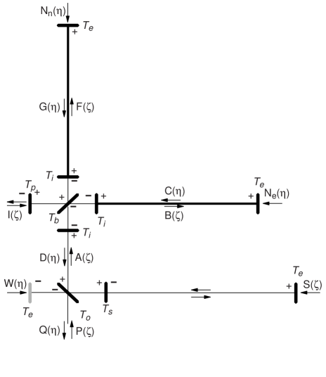
FIG. 3.: Schematic diagram showing the practical version of the three-cavity speed-meter design, which reduces the power flowing through the beam splitter. Three additional mirrors, with transmissivity $T_{\rm i}$, are placed around the beam splitter. The “$+$” and “$-$” signs near the mirrors indicate the sign of the reflectivities in the junction conditions for each location. The mirror shown in gray closes the second port of the interferometer.

As claimed by Mizuno [15] and tested experimentally by Freise et al. [16] and Mason [17], when the transmissivity of the third mirror decreases from $1$, the storage time of sideband fields in the arm cavity due to the presence of the internal mirrors will decrease. This phenomenon is called Resonant Sideband Extraction (RSE); consequently, the third mirror is called the RSE mirror. One special case, which is of great interest to us, occurs when the RSE mirror has the same transmissivity as the internal mirrors. In this case, the effect of the internal mirrors on the gravitational-wave sidebands should be exactly cancelled out by the RSE mirror. The three new mirrors then have just one effect: they reduce the carrier power passing through the beam splitter—and they can do so by a large factor.

Indeed, we have confirmed that this is true for our speed meter, as long as the distances between the three additional mirrors (the length of the “RSE cavity”) are small (a few meters), so that the phase shifts added to the slightly off-resonance sidebands by the RSE cavity are negligible. We can then adjust the transmissivities of the power-recycling mirror and of the three internal mirrors to reduce the amount of carrier power passing through the beam splitter to a more reasonable level.

With this design, the high circulating power is confined to the Fabry-Perot arm cavities, as in conventional LIGO designs. There is some question as to the level of power that mirrors will be able to tolerate in the LIGO-III time frame. Assuming that several megawatts is not acceptable, we shall show that the circulating power can be reduced by injecting fixed-angle squeezed vacuum into the dark port, as indicated by Eq. (3).

Going a step farther, we shall show that if, in addition to injected squeezed vacuum, we also use frequency-dependent (FD) homodyne detection, the sensitivity of the speed meter is dramatically improved at high frequencies (above $f_{\rm opt}\simeq 100$ Hz); this is shown in Fig. 1. The disadvantage of this is that FD homodyne detection requires two filter cavities of the same length as the arm cavities (4 km for LIGO), as shown in Fig. 4.

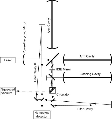
FIG. 4.: Schematic diagram showing the practical three-cavity speed-meter design with squeezed vacuum injected at the dark port and two filter cavities on the output. Note that the circulator is a four-port optical device that separates the injected (squeezed) input and the interferometer’s output.

Our analysis of the losses in these scenarios indicates that our speed meters with squeezed vacuum and/or variational-output are much less sensistive to losses than a position meter using those techniques (as analyzed by KLMTV). Losses for the various speed meters we discuss here are generally quite low and are due primarily to the losses in the optical elements (as opposed to mode-mismatching effects). Without squeezed vacuum, the losses in sensitivity are less than 10% in the range $50-105~{}\rm Hz$, lower at higher frequencies, but higher at low frequencies. Injecting fixed-angle squeezed vacuum into the dark port allows this speed meter to operate at a lower power [see Eq. 3], thereby reducing the dominant losses (which are dependent on the circulating power because they come from vacuum fluctations contributing to the back-action). In this case, the losses are less than 4% in the range $25-150~{}\rm Hz$. As before, they are lower at high frequencies, but they increase at low frequencies. Using FD homodyne detection does not change the losses significantly.

This paper is organized as follows: In Sec. II we give a brief description of the mathematical method that we use to analyze the interferometer. In Sec. III A, we present the results in the lossless case, followed in Sec. III B by a discussion of optimization methods. In Sec. III C, we discuss some of the advantages and disadvantages of this design, including the reasons it requires a large circulating power. Then in Sec. IV, we show how the circulating power can be reduced by injecting squeezed vacuum through the dark port of the interferometer and how the use of frequency-dependent homodyne detection can improve the performance at high frequencies. In Section V, we discuss the effect of losses on our speed meter with the various modifications made in Sec. IV, and we compare our interferometer configurations with those of KLMTV. Finally, we summarize our results in Sec. VI.

II Mathematical Description of the Interferometer

The interferometers in this paper are analyzed using the techniques described in Paper I (Sec. II). These methods are based on the formalism developed by Caves and Schumaker [18, 19] and used by KLMTV to examine more conventional interferometer designs. For completeness, we will summarize the main points here.

The electric field propagating in each direction down each segment of the interferometer is expressed in the form

$$E_{\rm field}(\zeta)=\sqrt{\frac{4\pi\hbar\omega_{0}}{{\cal S}c}}A(\zeta)\,.$$ (4)

Here $A(\zeta)$ is the amplitude (which is denoted by other letters—$B(\zeta)$, $P(\zeta)$, etc.—in other parts of the interferometer; see Fig. 2), $\zeta=t-z/c$, $\omega_{0}$ is the carrier frequency, $\hbar$ is the reduced Planck’s constant, and ${\cal S}$ is the effective cross-sectional area of the light beam; see Eq. (8) of KLMTV. For light propagating in the negative $z$ direction, $\zeta=t-z/c$ is replaced by $\eta=t+z/c$. We decompose the amplitude into cosine and sine quadratures,

$$A(\zeta)={\cal A}_{1}(\zeta)\cos\omega_{0}\zeta+{\cal A}_{2}(\zeta)\sin\omega_{0}\zeta\,,$$ (5)

where the subscript 1 always refers to the cosine quadrature, and 2 to sine. Both arms and the sloshing cavity have length $L=4$ km, whereas all of the other lengths $z_{i}$ are short compared to $L$. We choose the cavity lengths to be exact half multiples of the carrier wavelength so $e^{i2\omega_{0}L/c}=1$ and $e^{i2\omega_{0}z_{i}/c}=1$. There will be phase shifts put onto the sideband light in all of these cavities, but only the phase shifts due to the long cavities are significant.

The aforementioned sidebands are put onto the carrier by the mirror motions and by vacuum fluctuations. We express the quadrature amplitudes for the carrier plus the side bands in the form

$${\cal A}_{j}(\zeta)=A_{j}(\zeta)+\int_{0}^{\infty}\bigl{[}\tilde{a}_{j}(\omega)e^{-i\omega\zeta}+\tilde{a}_{j}^{\dagger}(\omega)e^{i\omega\zeta}\bigr{]}\frac{d\omega}{2\pi}\,.$$ (6)

Here $A_{j}(\zeta)$ is the carrier amplitude, $\tilde{a}_{j}(\omega)$ is the field amplitude (a quantum mechanical operator) for the sideband at sideband frequency $\omega$ (absolute frequency $\omega_{0}\pm\omega$) in the $j$ quadrature, and $\tilde{a}_{j}^{\dagger}(\omega)$ is the Hermitian adjoint of $\tilde{a}_{j}(\omega)$; cf. Eqs. (6)–(8) of KLMTV, where commutation relations and the connection to creation and annihilation operators are discussed. In other portions of the interferometer (Fig. 2), ${\cal A}_{j}(\zeta)$ is replaced by, e.g., ${\cal C}_{j}(\zeta)$; $A_{j}(\zeta)$, by $C_{j}(\zeta)$; $\tilde{a}_{j}(\omega)$, by $\tilde{c}_{j}(\omega)$, etc.

Since each mirror has a power transmissivity and complementary reflectivity satisfying the equation $T+R=1$, we can write out the junction conditions for each mirror in the system, for both the carrier quadratures and the sidebands [see particularly Eqs. (5) and (12)–(14) in Paper I]. We shall denote the power transmissivities for the sloshing mirror as $T_{\rm s}$, for the extraction (output) mirror as $T_{\rm o}$, the power-recycling mirror as $T_{\rm p}$, for the beam-splitter as $T_{\rm b}=0.5$, for the internal mirrors as $T_{\rm i}$, and for the end mirrors as $T_{\rm e}$; see Figs. 2 and 3.

The resulting equations can be solved simultaneously to get expressions for the carrier and sidebands in each segment of the interferometer. Since those expressions may be quite complicated, we use the following assumptions to simplify our results. First, we assume that only the cosine quadrature is being driven (so that the carrier sine quadrature terms are all zero). Second, we assume that the transmissivities obey

$$1\gg T_{\rm o}\gg T_{\rm s}\gg T_{\rm e}\quad{\rm and}\quad 1\gg\{T_{\rm p},T_{\rm i}\}\gg T_{\rm e}\,.$$ (7)

The motivations for these assumptions are that (i) they lead to speed-meter behavior; (ii) as with any interferometer, the best performance is achieved by making the end-mirror transmissivities $T_{\rm e}$ as small as possible; and (iii) good performance requires a light extraction rate comparable to the sloshing rate, $\delta\sim\Omega$ [cf. the first paragraph of Sec. III B in Paper I], which with Eqs. (1) and (2) implies $T_{\rm o}\sim\sqrt{T_{\rm s}}$ so $T_{\rm o}\gg T_{\rm s}$. Throughout the paper, we will be using these assumptions, together with $\omega L/c\ll 1$, to simplify our expressions.

III Speed Meter in the Lossless Limit

For simplicity, in this section we will set $T_{\rm e}=0$ (end mirrors perfectly reflecting). We will also neglect the (vacuum-fluctuation) noise coming in the main laser port ($\tilde{i}_{1,2}$) since that noise largely exits back toward the laser and produces negligible noise on the signal light exiting the output port. As a result of these assumptions, the only (vacuum-fluctuation) noise that remains is that which comes in through the output port ($\tilde{p}_{1,2}$). An interferometer in which this is the case and in which light absorption and scattering are unimportant ($R+T=1$ for all mirrors, as we have assumed) is said to be “lossless.” In Sec. V, we shall relax these assumptions; i.e., we shall consider lossy interferometers.

It should be noted that the results and discussion in this section and in Sec. IV apply to both the simple and practical versions of the three-cavity speed meter (Figs. 2 and 3). The two versions are completely equivalent (in the lossless limit).

A Mathematical Analysis

The lossless interferometer output for the speed meters in Fig. 2 and 3, as derived by the analysis sketched in the previous section, is then

$$\tilde{q}_{1} = -{{\cal L}^{*}(\omega)\over{\cal L}(\omega)}\tilde{p}_{1}\,,$$ (9)

$$\tilde{q}_{2} = \frac{2i\omega\sqrt{\omega_{0}\delta W_{\rm circ}}}{\sqrt{\hbar cL}{\cal L}(\omega)}\tilde{x}-\frac{{\cal L}^{\ast}(\omega)}{{\cal L}(\omega)}\tilde{p}_{2}\,.$$ (10)

Here $\tilde{p}_{j}(\omega)$ is the side-band field operator [analog of $\tilde{a}_{j}(\omega)$ in Eq. (6)] associated with the dark-port input $P(\zeta)$, and $\tilde{q}_{j}(\omega)$ associated with the output $Q(\eta)$; see Fig. 2. Also, in Eqs. (III A), ${\cal L}(\omega)$ is a c-number given by

$${\cal L}(\omega)=\Omega^{2}-\omega^{2}-i\omega\delta$$ (11)

[recalling that $\Omega=c\sqrt{T_{\rm s}}/2L$ is the sloshing frequency, $\delta=cT_{\rm o}/L$ the extraction rate], the asterisk in ${\cal L}^{\ast}(\omega)$ denotes the complex conjugate, $\tilde{x}(\omega)$ is the Fourier transform of the relative displacement of the four test masses—i.e., the Fourier transform of the difference in lengths of the interferometer’s two arm cavities—and $W_{\rm circ}$ is the circulating power in the each of the interferometer’s two arms. Note that the circulating power (derived as in Sec. II B of Paper I) is related to the carrier amplitude $B_{1}$ in the arms by

$$W_{\rm circ}=\frac{1}{2}\hbar\omega_{0}B_{1}^{2}=\frac{4\hbar\omega_{0}I_{1}^{2}}{T_{\rm i}T_{\rm p}}\,,$$ (12)

where $I_{1}$ is the input laser amplitude (in the cosine quadrature). Readers who wish to derive the input–output relations (III A) for themselves may find useful guidance in Appendix B of KLMTV [7] and in Secs. II and III of Paper I [8], which give detailed derivations for other interferometer designs.

Notice that the first term in Eq. (10) contains $\tilde{x}$ only in the form $\omega\tilde{x}$; this is the velocity signal [actually, the sum of the velocity and higher odd time derivatives of position because of the ${\cal L}(\omega)$ in the denominator]. The test masses’ relative displacement $\tilde{x}(\omega)$ is given by

$$\tilde{x}=\tilde{x}_{e}-\tilde{x}_{n}=L\tilde{h}-\frac{8i\sqrt{\hbar\omega_{0}\delta W_{\rm circ}}}{m\omega\sqrt{cL}{\cal L}(\omega)}\tilde{p}_{1}\,,$$ (13)

where $\tilde{x}_{e}$ is the Fourier transform of the relative displacement of the mirrors of the “east” arm and $\tilde{x}_{n}$ is the same for the “north” arm. The last term is the back-action produced by fluctuating radiation pressure (derived as in Sec. II B of Paper I).

It is possible to express Eqs. (III A) in a more concise form, similar to Eqs. (16) in KLMTV:

$$\tilde{q}_{1} = \Delta\tilde{p}_{1}=\tilde{p}_{1}e^{2i\psi}\,,$$ (15)

$$\tilde{q}_{2} = \Delta\tilde{p}_{2}+\sqrt{2\kappa}\frac{\tilde{h}}{h_{SQL}}e^{i\psi}\,,\quad\Delta\tilde{p}_{2}=(\tilde{p}_{2}-\kappa\tilde{p}_{1})e^{2i\psi}\,.$$ (16)

Here

$$\tan\psi=-\frac{\Omega^{2}-\omega^{2}}{\omega\delta}$$ (17)

is a phase shift put onto the light by the interferometer,

$$\kappa=\frac{16\omega_{0}\delta W_{\rm circ}}{mcL|{\cal L}(\omega)|^{2}}$$ (18)

is a dimensionless coupling constant that couples the gravity wave signal $\tilde{h}$ into the output $\tilde{q}_{2}$, and

$$h_{SQL}=\sqrt{\frac{8\hbar}{m\omega^{2}L^{2}}}$$ (19)

is the standard quantum limit for a conventional interferometer such as LIGO-I or VIRGO [1].

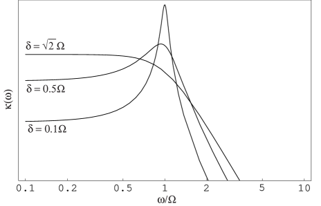
FIG. 5.: The coupling constant $\kappa(\omega)$ in arbitrary (logrithmic) units with $\omega$ measured in units of $\Omega$. The three curves correspond to the same light power (such that $\kappa_{\rm max}=5$ for the middle curve), but $\delta=0.1\Omega$, $\delta=0.5\Omega$, and $\delta=\sqrt{2}\Omega$.

In Fig. 5, we plot the coupling constant $\kappa$ as a function of frequency for several values of $\delta$. As the graph shows, $\kappa$ can be roughly constant for a rather broad frequency band $\omega\stackrel{{\scriptstyle<}}{{{}_{\sim}}}\Omega$, when $\delta$ is chosen to be $\sim\Omega$ (as it will be when the interferometer is optimized). Combining this with the fact that $h_{SQL}\propto 1/\omega$, we infer from Eqs. (III A) that the output signal at frequencies $\omega\lesssim\Omega$ is proportional to $\omega\tilde{h}$, or equivalently $\omega\tilde{x}$, which is the relative speed of the test masses (as mentioned above).

The terms $\Delta\tilde{p}_{1}$ and $\Delta\tilde{p}_{2}$ in Eqs. (III A) represent quantum noise (shot noise, radiation-pressure noise, and their correlations). We shall demonstrate below that, in the frequency band $\omega\lesssim\Omega$ where the interferometer samples only the speed, there is no back-action (radiation-pressure) noise. This might not be obvious from Eqs. (III A), especially because they have an identical form (except for the frequency dependence of $\kappa$) as the input-output relations of a conventional interferometer, where the term proportional to $\cal K$ (their version of $\kappa$) is the radiation-pressure noise. Indeed, if one measures the “sine” quadrature of the output, $\tilde{q}_{2}$, as is done in a conventional interferometer, this speed meter turns out to be SQL limited, as are conventional interferometers.

Fortunately, the fact that $\kappa$ is constant (and equal to $\kappa_{0}$) over a broad frequency band will allow the aforementioned cancellation of the back-action, resulting in a QND measurement of speed. To see this, suppose that, instead of measuring the output phase quadrature $\tilde{q}_{2}$, we use homodyne detection to measure a generic, frequency-independent quadrature of the output:

$$\tilde{q}_{\Phi}=\Delta\tilde{p}_{1}\cos\Phi+(\Delta\tilde{p}_{2}+\sqrt{2\kappa}\frac{h}{h_{SQL}}e^{i\psi})\sin\Phi\,,$$ (20)

where $\Phi$ is a fixed homodyne angle. Then from Eqs. (III A), we infer that the noise in the signal, expressed in GW strain units $h$, is

$$h_{n}=\frac{h_{SQL}}{\sqrt{2\kappa}}e^{i\psi}[\tilde{p}_{1}(\cot\Phi-\kappa)+\tilde{p}_{2}]\,.$$ (21)

By making $\cot\Phi=\kappa_{0}\equiv({\rm constant\ value\ of\ \kappa\ at\ \omega\lesssim\Omega})$, the radiation pressure noise in $h_{n}$ will be cancelled in the broad band where $\kappa=\kappa_{0}$, thereby making this a QND interferometer.

We assume for now that ordinary vacuum enters the output port of the interferometer; i.e., $\tilde{p}_{1}$ and $\tilde{p}_{2}$ are quadrature amplitudes for ordinary vacuum (we will inject squeezed vacuum in Sec. IV A). This means [Eq. (26) of KLMTV] that their (single-sided) spectral densities are unity and their cross-correlations are zero, which, when combined with Eq. (21), implies a spectral density of

$$S_{h_{n}}=(h_{SQL})^{2}\xi^{2}\,.$$ (22)

Here

$$\xi^{2}\equiv\frac{(\cot\Phi-\kappa)^{2}+1}{2\kappa}$$ (23)

is the fractional amount by which the SQL is beaten (in units of squared amplitude). This expression for $\xi^{2}$ is the same as that for the speed meters in Paper I [Eq. (35)] and BGKT [Eq. (40)], indicating the theoretical equivalency of these designs. In those papers, an optimization is given for the interferometer. Instead of just using the results of that optimization, we shall carry out a more comprehensive study of it.

B Optimization

The possible choices of speed meter parameters can be investigated intuitively by examining the behavior of $\kappa$. To aid us in our exploration, we choose (as in BGKT and Paper I) to express $|{\cal L}(\omega)|^{2}$ [Eq. (11)] as

$$|{\cal L}(\omega)|^{2}=(\omega^{2}-\omega_{\rm opt}^{2})^{2}+\delta^{2}(\omega^{2}_{\rm opt}+\delta^{2}/4)\,,$$ (24)

where

$$\omega_{\rm opt}=\sqrt{\Omega^{2}-\delta^{2}/2}\,,$$ (25)

is the interferometer’s “optimal frequency,” i.e., the frequency at which $|{\cal L}(\omega)|$ reaches its minimum. Combining with Eq. (18), we obtain

$$\kappa=\frac{\Omega_{\rm I}^{3}\,\delta}{(\omega^{2}-\omega_{\rm opt}^{2})^{2}+\delta^{2}(\omega^{2}_{\rm opt}+\delta^{2}/4)}\,,$$ (26)

where

$$\Omega_{\rm I}^{3}\equiv\frac{16\omega_{0}W_{\rm circ}}{mLc}$$ (27)

is a frequency scale related to the circulating power. At $\omega_{\rm opt}$, $\kappa$ reaches its maximum (see Fig. 6)

$$\kappa_{\rm max}=\frac{\Omega_{\rm I}^{3}}{\delta(\omega_{\rm opt}^{2}+\delta^{2}/4)}\,.$$ (28)

By setting

$$\cot\Phi=\kappa_{\rm max}\,,$$ (29)

we get the maximum amount by which a speed meter can beat the SQL

$$\xi_{\rm min}^{2}=\frac{1}{2\kappa_{\rm max}}=\frac{\delta(\omega_{\rm opt}^{2}+\delta^{2}/4)}{2\Omega_{\rm I}^{3}}\,.$$ (30)

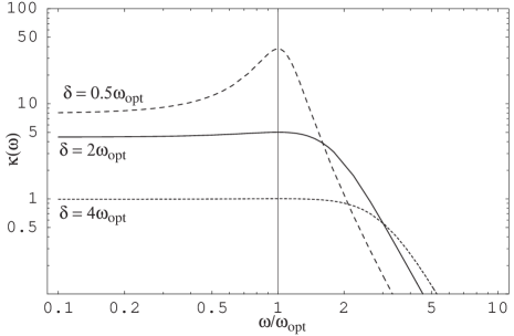
FIG. 6.: The coupling constant $\kappa(\omega)$ with $\omega$ measured in units of $\omega_{\rm opt}$. The solid curve is determined by setting $\delta=2\omega_{\rm opt}$ and $\kappa_{\rm max}=5$ (this value of $\kappa_{\rm max}$ comes from specifying that we want to beat the SQL by a factor of 10; see Fig. 8). If, in addition, we set $\omega_{\rm opt}=2\pi\times 100~{}\rm Hz$, then all the parameters have been specified (due to the various relationships between them) and are equal to the values given in Table I. If we maintain the same power but change $\delta$, then the only parameter of Table I that is affected is $T_{\rm o}$. Examples of such a change are shown for $\delta=0.5\omega_{\rm opt}$ and $\delta=4\omega_{\rm opt}$. Note that these two choices of $\delta$ are more extreme than would be desirable in practice, but they are shown here to illustrate more clearly the effect on $\kappa$ of changing the ratio between $\delta$ and $\omega_{\rm opt}$.

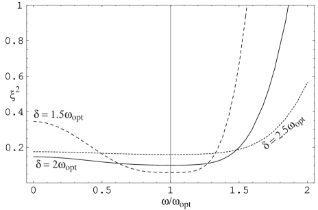
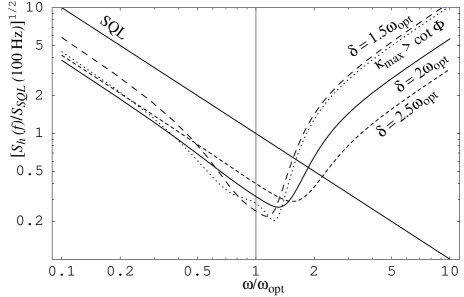
FIG. 7.: The squared amount by which the speed meter beats the SQL with a given circulating power, which is determined by setting (for the solid curve) $\xi^{2}_{\rm min}=0.1$ and the condition (33). Note that the requirement on $\xi_{\rm min}^{2}$ sets the power relative to the SQL power $W_{\rm circ}^{SQL}$, the value of which is dependent on $\omega_{\rm opt}$. (For $\omega_{\rm opt}=100~{}\rm Hz$, we have $W_{\rm circ}=8~{}\rm MW$.) If we hold the power fixed and change $\delta$ to $1.5\omega_{\rm opt}$ and $2.5\omega_{\rm opt}$, we get the other two curves.

FIG. 8.: Noise curves corresponding to the $\xi^{2}$ curves in Fig. 8, the caption of which describes the parameters used here as well. The dotted line is an example of a noise curve for which $\kappa$ is not quite flat and $\cot\Phi$ was chosen to be slightly smaller than $\kappa_{\rm max}$ (see the end of Sec. III B for details.)

As $\omega$ differs from $\omega_{\rm opt}$ in either direction, $\kappa$ decreases from $\kappa_{\rm max}$. This causes the noise to increase since (i) the term $(\cot\Phi-\kappa)^{2}$ in the numerator of $\xi^{2}$ [Eq. (23)] increases and (ii) the denominator of $\xi^{2}$ decreases. In order to have broadband performance, we should make the peak of $\kappa(\omega)$ as flat as possible. As we can see from both Eq. (26) and Fig. 6, the shape of the peak can be adjusted by changing $\delta$: for the same optical power, a larger $\delta$ means a wider peak but a smaller maximum. Therefore, changing $\delta$ is one method of balancing sensitivity against bandwidth. Some examples are shown in Figs. 6, 8, and 8, where $\kappa(\omega)$, $\xi^{2}(\omega)$, and $S_{h}(\omega)$, respectively, are plotted for configurations with the same $\omega_{\rm opt}$ and optical power $W_{\rm circ}$, but with several values of $\delta$.

To be more quantitative, a simple analytic form for $\xi^{2}(\omega)$ can be obtained by inserting Eqs. (26), (28), and (30) into Eq. (23) to get

$$\xi^{2}(\omega)=\left[1+\Delta+\frac{1}{4\xi_{\rm min}^{4}}\frac{\Delta^{2}}{(1+\Delta)}\right]\xi_{\rm min}^{2}\,.$$ (31)

Here

$$\Delta\equiv\frac{\left(\omega^{2}-\omega_{\rm opt}^{2}\right)^{2}}{\delta^{2}(\omega_{\rm opt}^{2}+\delta^{2}/4)}\,$$ (32)

is a dimensionless offset from the optimal frequency $\omega_{\rm opt}$. From Eq. (32), it is evident that $\Delta$, and thus $\xi^{2}$, are the same for $\omega=0$ and $\omega=\sqrt{2}\omega_{\rm opt}$ [see also Eq. (47) of BGKT or Eq. (49) of Paper I]. For definiteness, let us impose that

$$\xi^{2}(0)=\xi^{2}(\sqrt{2}\omega_{\rm opt})=\frac{3}{2}\xi^{2}_{\rm min}$$ (33)

as is done by BGKT. For $\xi_{\rm min}^{2}=0.1$, this gives $\delta=1.977\omega_{\rm opt}\approx 2\omega_{\rm opt}$ (as assumed in BGKT and Paper I). Plugging these numbers into Eq. (30) and combining with Eq. (27) gives

$$W_{\rm circ} ({\delta=2\omega_{\rm opt}})=\frac{mLc\,\omega_{\rm opt}^{3}}{8\omega_{0}\xi_{\rm min}^{2}}$$ (36)

$$\simeq 8.4\,{\rm MW}\left(\frac{\omega_{\rm opt}}{2\,\pi\times 100\,{\rm Hz}}\right)^{3}\left(\frac{m}{40\,{\rm kg}}\right)$$

$$\quad\times\left(\frac{L}{4000\,{\rm km}}\right)\left(\frac{1.78\times 10^{15}\,{\rm Hz}}{\omega_{0}}\right)\left(\frac{0.1}{\xi_{\rm min}^{2}}\right)\,.$$

Therefore, when $\omega_{\rm opt}$ is chosen at $2\pi\times 100\,{\rm Hz}$, this speed meter (with $\delta=2\omega_{\rm opt}$) requires $W_{\rm circ}\simeq 8.4\,{\rm MW}$ to beat the SQL by a factor of 10 in power ($\xi_{\rm min}^{2}=0.1$). [Note that, keeping $\delta=2\omega_{\rm opt}$, the speed meter reaches the SQL with $W_{\rm circ}^{\rm SQL}=840\,{\rm kW}$, comparable to the value given by KLMTV Eq. (132) for conventional interferometers with 40-kilogram test masses.] The $\xi^{2}$ and $S_{h}$ curves for this configuration are plotted as solid lines in Fig. 8 and 8, respectively.

Please note that Eq. (36) should be applied with caution because significantly changing $\xi^{2}_{\rm min}$ in the above equation (without changing the ratio between $\delta$ and $\omega_{\rm opt}$) will change the wide-band performance of the interferometer, since there is some “hidden” power dependence in Eq. (33). To determine the behavior of the speed meter with significantly higher power or lower $\xi_{\rm min}^{2}$ while maintaining the same wideband performance, we must re-apply the requirement (33) to determine the appropriate ratio between $\delta$ and $\omega_{\rm opt}$. For example, solving Eqs. (30) and (33) simultaneously for $\xi^{2}_{\rm min}$ and $\delta$, with chosen values $W_{\rm circ}=20~{}{\rm MW}$ and $\omega_{\rm opt}=2\pi\times 100~{}{\rm Hz}$, gives $\delta=2.334\omega_{\rm opt}$ and $\xi_{\rm min}^{-2}\simeq 17$. Keeping this in mind, a general expression for the circulating power is

$$W_{\rm circ} = \frac{mLc(\omega_{\rm opt}^{2}+\delta^{2}/4)\delta}{32\omega_{0}\,\xi_{\rm min}^{2}}$$ (37)

$$= \frac{209\,{\rm kW}}{\xi_{\rm min}^{2}}\left[\frac{(\omega_{\rm opt}^{2}+\delta^{2}/4)\delta}{(2\pi\times 100\,{\rm Hz})^{3}}\right]$$ (39)

$$\times\left(\frac{m}{40\,{\rm kg}}\right)\left(\frac{L}{4000\,{\rm km}}\right)\left(\frac{1.78\times 10^{15}\,{\rm Hz}}{\omega_{0}}\right)\,,$$

where the relationship between $\delta$ and $\omega_{\rm opt}$ determines whether the noise curve is deep but narrow or wide but shallow [with the requirement (33) giving the latter].

So far, we have only changed $\delta$ to modify the performance of the speed meter. Another method is to change $\omega_{\rm opt}$. In this case, the shape of the noise curve changes very little, but the minima occur at different frequencies, causing the interferometer to have either broader bandwidth or higher sensitivity (relative to the SQL). This is shown in Fig. 9. Maintaining condition (33) with $\omega_{\rm opt}$ chosen at $2\pi\times 150$ Hz, we get a broader but shallower curve (short dashes); this configuration beats the SQL by a factor of $\xi_{\rm min}^{-2}\sim 4.7$, up to $f\sim 240\,{\rm Hz}$. With $\omega_{\rm opt}=2\pi\times 75$ Hz, we get a narrower but deeper curve (long dashes), which beats the SQL by a factor of $\xi_{\rm min}^{-2}\sim 17$, up to $f\sim 100\,{\rm Hz}$. The power was kept fixed at $W_{\rm circ}=8.2\,{\rm MW}$.

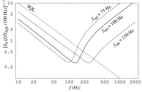
FIG. 9.: Noise curves for varying optimal frequencies. The solid curve has $f_{\rm opt}=100$ Hz and is identical to the solid curve of Fig. 8. Maintaining the same power and the condition imposed by Eq. (33), we show two examples of noise curves with other optimal frequencies, specifically $f_{\rm opt}=75$ Hz and $f_{\rm opt}=150$ Hz.

One more potential optimization method is to choose a $\kappa$ with a peak that is not quite flat and then choose a $\cot\Phi$ that is slightly smaller than $\kappa_{\rm max}$. This will give a wider bandwidth on either side of $\omega_{\rm opt}$, at the price of decreased sensitivity at the region near $\omega_{\rm opt}$ (see dotted line in Fig. 8).

For simplicity, we will choose a typical (but somewhat arbitrary) set of parameters for the lossless interferometer of Fig. 2. These values, given in Table I, will be used (except as otherwise noted) for subsequent plots and calculations comparing this speed-meter design to other configurations.

TABLE I.: Three-arm speed-meter interferometer parameters and their fiducial values, as used throughout except where other parameters are specified.

Parameter	Symbol	Fiducial Value
carrier frequency	$\omega_{0}$	$1.78\times 10^{15}{\rm s}^{-1}$
mirror mass	$m$	40 kg
arm length	$L$	4 km
sloshing mirror transmissivity	$T_{\rm s}$	0.0008
output mirror transmissivity	$T_{\rm o}$	0.017
end mirror transmissivity	$T_{\rm e}$	$2\times 10^{-5}$
internal and RSE mirror trans.	$T_{\rm i}$	0.005
optimal frequency	$\omega_{\rm opt}$	$2\pi\times 100~{}\rm Hz$
sloshing frequency	$\Omega$	$2\pi\times 170~{}\rm Hz$
extraction rate (half-bandwidth)	$\delta$	$2\pi\times 200~{}\rm Hz$
SQL circulating power	$W_{\rm circ}^{SQL}$	820 kW

C Discussion of Three-Cavity Speed-Meter Design

In this section, we discuss how the three-cavity speed-meter design compares to the two-cavity design presented in Paper I, focusing on the three major problems of that design: it required (i) a high circulating power, (ii) a large amount of power coming out of the interferometer with the signal, and (iii) an exorbitantly high input laser power.

With the three-cavity speed meter, we are able to replicate the performance of the two-cavity design in Paper I, but without the exorbitantly high input power. The reason why our three-cavity speed meter does not need a high input power is the same as for conventional interferometers: in both cases, the excited cavities are fed directly by the laser. According to Bose statistics, carrier photons will be “sucked” into the cavities, producing a strong amplification. This was not the case in the two-cavity speed meter of Paper I. There, an essentially empty cavity stood between the input and the excited cavity, thereby thwarting Bose statistics and resulting in a required input laser power much greater than the power that was circulating in the excited cavity (see Paper I for more details). In this paper, we have returned to a case where the laser is driving an excited cavity directly, thereby allowing the input laser power to be small relative to the circulating power.

Because the cavity from which we are reading out the signal does not contain large amounts of carrier light (by contrast with the two-cavity design), this three-cavity speed meter does not have large amounts of power exiting the interferometer with the velocity signal, unlike the two-cavity design. By making use of the different modes of the Michelson interferometer, we have solved the problem of the exorbitantly high input power and the problem of the amount of light that comes out of the interferometer.

The problem of the high circulating power $W_{\rm circ}$, unfortunately, is not solved by the three-cavity design. This is actually a common characteristic of “external-readout” interferometer designs capable of beating the SQL. The reason for this high power is the energetic quantum limit (EQL), which was first derived for gravitational-wave interferometers by Braginsky, Gorodetsky, Khalili and Thorne [20]. The EQL arises from the phase-energy uncertainty principle

$$\Delta E\Delta\phi\geq\frac{\hbar\omega_{0}}{2}\,,$$ (40)

where $E$ is the stored energy in the interferometer and $\phi$ is the phase of the light. The uncertainty $\Delta E$ of the stored light energy during the measurement process must be large enough to allow a small uncertainty $\Delta\phi$ in the stored light’s optical phase, in which the GW signal is contained. For an interferometer with coherent light (so $\Delta E=\hbar\omega_{0}\sqrt{E/\hbar\omega_{0}}$), the EQL dictates that the energy stored in the arms must be larger than

$$E_{\rm\xi}\sim\frac{mL^{2}\omega^{2}\Delta\omega}{4\omega_{0}\xi^{2}}\,$$ (41)

in order to beat the SQL by a factor of $\xi$ near frequency $\omega$ with a bandwidth $\Delta\omega$ (Eq. (1) of Ref. [11] and Eq. (29) of Ref. [20]). In a broadband configuration with $\Delta\omega\sim\omega$, we have

$$E_{\rm\xi}\sim\frac{mL^{2}\omega^{3}}{4\omega_{0}\xi^{2}}\,.$$ (42)

For comparison, in the broadband regime of the speed meter, we have, from Eq. (30),

$$\xi_{\rm min}^{2}=\frac{mL^{2}\delta(\omega_{\rm opt}^{2}+\delta^{2}/4)}{4\,E\omega_{0}}\sim\frac{mL^{2}\omega_{\rm opt}^{3}}{4\,E\omega_{0}}\,,$$ (43)

where the stored energy is $E=2W_{\rm circ}L/c$. Comparison between Eqs. (42) and (43) confirms that our speed meter is EQL limited.

As a consequence of the EQL, designs with coherent light will all require a similarly high circulating power in order to achieve a similar sensitivity. Moreover, given the sharp dependence $E\propto\omega^{3}$, this circulating power problem will become much more severe when one wants to improve sensitivities at high frequencies.

Nevertheless, the EQL in the form (41) above only applies to coherent light. Using nonclassical light will enable the interferometer to circumvent it substantially. One possible method was invented by Braginsky, Gorodetsky, and Khalili [10] using a special optical topology and intracavity signal extraction. A more conventional solution for our external-readout interferometer is to inject squeezed light into the dark port, as we shall discuss in Sec. IV A (and as was also discussed in the original paper [20] on the EQL).

IV Squeezed Vacuum and FD Homodyne Dectection

In this section, we discuss two modifications to the three-cavity speed-meter design analyzed in Sec. III A. This discussion applies to both the simple and practical versions, shown in Figs. 2 and 3; the modifications are shown in Fig. 4. The first modification is to inject squeezed vacuum (with fixed squeeze angle) into the output port of the speed meter, as shown in Fig. 4. This will reduce the amount of power circulating in the interferometer. The second modification, also shown in Fig. 4, is the introduction of two filter cavities on the output, which allow us to perform frequency-dependent homodyne detection (described in KLMTV) that will dramatically improve the performance of the speed meter at frequencies $f\gtrsim f_{\rm opt}$.

A Injection of Squeezed Vacuum into Dark Port

Because the amount of circulating power required by our speed meter remains uncomfortably large, it is desirable to reduce it by injecting squeezed vacuum into the dark port. The idea of using squeezed light in gravitational-wave interferometers was first conceived by Caves [14] and further developed by Unruh [4] and KLMTV. We shall start in this section with a straightforward scheme that will decrease the effective circulating power without otherwise changing the speed meter performance.

As discussed in Sec. IV B and Appendix A of KLMTV, a squeezed input state is related to the vacuum input state (assumed in Sec. III A) by a unitary squeeze operator $S(R,\lambda)$ [see Eqs. (41) and (A5) of KLMTV]

$$|{\rm in}\rangle=S(R,\lambda)|0\rangle\,.$$ (44)

Here $R$ is the squeeze amplitude and $\lambda$ is the squeeze angle, both of which in principle can depend on sideband frequency. However, the squeezed light generated using nonlinear crystals [21, 22] has frequency-independent $R$ and $\lambda$ in our frequency band of interest, i.e., $f<10$ kHz [23]; and in this section, we shall assume frequency independence.

The effect of input squeezing is most easily understood in terms of the following unitary transformation,

$$|{\rm in}\rangle \rightarrow S^{\dagger}(R,\lambda)|{\rm in}\rangle=|0\rangle\,$$ (46)

$$\tilde{p}_{j} \rightarrow S^{\dagger}(R,\lambda)\tilde{p}_{j}S(R,\lambda)\,,$$ (47)

$$\tilde{q}_{j} \rightarrow S^{\dagger}(R,\lambda)\tilde{q}_{j}S(R,\lambda)\,,$$ (48)

where $j=1,2$. This brings the input state back to vacuum and transforms the input quadratures into linear combinations of themselves, in a rotate-squeeze-rotate way [Eq. (A8) of KLMTV, in matrix form]:

$$\left(\begin{array}[]{c}\tilde{p}_{1}\\ \tilde{p}_{2}\end{array}\right) \rightarrow \left(\begin{array}[]{c}\tilde{p}_{1s}\\ \tilde{p}_{2s}\end{array}\right)=S^{\dagger}(R,\lambda)\left(\begin{array}[]{c}\tilde{p}_{1}\\ \tilde{p}_{2}\end{array}\right)S(R,\lambda)$$ (65)

$$\quad=\left(\begin{array}[]{rr}\cos\lambda&-\sin\lambda\\ \sin\lambda&\cos\lambda\end{array}\right)\left(\begin{array}[]{cc}e^{-R}&0\\ 0&e^{R}\end{array}\right)$$

$$\quad\quad\quad\times\left(\begin{array}[]{rr}\cos\lambda&\sin\lambda\\ -\sin\lambda&\cos\lambda\end{array}\right)\left(\begin{array}[]{c}\tilde{p}_{1}\\ \tilde{p}_{2}\end{array}\right)\,.$$

In particular, the GW noise can be calculated by using the squeezed noise operator [Eq. (29) of KLMTV]

$$h_{ns}=S^{\dagger}(R,\lambda)h_{n}S(R,\lambda)\,,$$ (66)

and the vacuum state.

A special case—the case that we want—occurs when $R={\rm constant}$ and $\lambda=\pi/2$. Then there is no rotation between the quadratures but only a frequency-independent squeezing or stretching,

$$\tilde{p}_{1} \rightarrow \tilde{p}_{1s}=e^{R}\tilde{p}_{1}\,,$$ (68)

$$\tilde{p}_{2} \rightarrow \tilde{p}_{2s}=e^{-R}\tilde{p}_{2}\,.$$ (69)

Consequently, Eqs. (III A) for the output quadratures $\tilde{q}_{1,2s}=S^{\dagger}(R,\pi/2)\tilde{q}_{1,2}S(R,\pi/2)$ are transformed into

$$\tilde{q}_{1s} = e^{R}\tilde{p}_{1}e^{2i\psi}$$ (71)

$$\tilde{q}_{2s} = e^{-R}\biggl{[}\left(\tilde{p}_{2}-\kappa e^{2R}\tilde{p}_{1}\right)e^{2i\psi}+\sqrt{\kappa e^{2R}}\frac{\tilde{h}}{h_{SQL}}e^{i\psi}\biggr{]}\,.$$ (72)

The corresponding noise can be put into the same form as Eq. (21),

$$h_{ns}=\frac{h_{SQL}}{\sqrt{\kappa_{\rm eff}}}e^{i\psi}\left[\tilde{p}_{1}(\cot\Phi_{\rm eff}-\kappa_{\rm eff})+\tilde{p}_{2}\right]\,,$$ (73)

with

$$\cot\Phi_{\rm eff}\equiv e^{2R}\cot\Phi\,,\quad\kappa_{\rm eff}\equiv e^{2R}\kappa\,.$$ (74)

Since $\kappa$ is proportional to the circulating power [see Eqs. (18)], gaining a factor $e^{2R}$ in $\kappa$ is equivalent to gaining this factor in $W_{\rm circ}$.

In other words, by injecting squeezed vacuum with squeeze factor $e^{2R}$ and squeeze angle $\lambda=\pi/2$ into the interferometer’s dark port, we can achieve precisely the same interferometer performance as in Sec. III A, but with a circulating light power that is lower by $W_{\rm circ,SISM}=e^{-2R}W_{\rm circ,OSM}$. (Here “SISM” means “squeezed-input speed meter” and “OSM” means “ordinary speed meter.” Since squeeze factors $e^{-2R}\sim 0.1$ are likely to be available in the time frame of LIGO-III [7], this squeezed-input speed meter can function with $W_{\rm circ,SISM}\simeq 0.1W_{\rm circ,OSM}$.

B Frequency-Dependent Homodyne Detection

One can take further advantage of squeezed light by using frequency-dependent (FD) homodyne detection at the interferometer output [24, 25, 26, 27, 28]. As KLMTV have shown, FD homodyne detection can be achieved by sending the output light through one or more optical filters (as in Fig. 4) and then performing ordinary homodyne detection. If its implemention is feasible, FD homodyne detection will dramatically improve the speed meter’s sensitivity at high frequencies (above $f_{\rm opt}=100$ Hz). Note that the KLMTV design that used FD homodyne detection was called a “variational-output” interferometer; consequently, we shall use the term “variational-output speed meter” to refer to our speed meter with FD homodyne detection. Continuing the analogy, when we have both squeezed-input and FD homodyne detection, we will use the term “squeezed-variational speed meter.” The following discussion is analogous to Secs. IV and V of KLMTV.

For a generic frequency-dependent squeeze angle $\lambda(\omega)$ and homodyne detection phase $\Phi(\omega)$, we have, for the squeezed noise operator [Eqs. (66) and (65)],

$$h_{ns}=-\frac{h_{SQL}}{\sqrt{\kappa}}e^{i\psi}\sqrt{1+\tilde{\kappa}^{2}}$$ (75)

$$\;\;\times\biggl{(}\tilde{p}_{1}\bigl{\{}\cosh R\cos\tilde{\Psi}-\sinh R\cos\bigl{[}\tilde{\Psi}-2(\tilde{\Psi}+\lambda)\bigr{]}\bigr{\}}$$ (76)

$$\;\;-\tilde{p}_{2}\bigl{\{}\cosh R\sin\tilde{\Psi}-\sinh R\sin\bigl{[}\tilde{\Psi}-2(\tilde{\Psi}+\lambda)\bigr{]}\bigr{\}}\biggr{)}\,,$$ (77)

where

$$\cot\tilde{\Psi}\equiv\tilde{\kappa}\equiv\kappa-\cot\Phi\,.$$ (78)

The corresponding noise spectral density [computed by using the ordinary vacuum spectral densities, $S_{\tilde{p}_{1}}=S_{\tilde{p}_{2}}=1$ and $S_{\tilde{p}_{1}\tilde{p}_{2}}=0$, in Eq. (77)] is

$$S_{h} = \frac{(h_{SQL})^{2}}{\kappa}(1+\tilde{\kappa}^{2})$$ (80)

$$\qquad\times\biggl{\{}e^{-2R}+\sinh 2R[1-\cos 2(\tilde{\Psi}+\lambda)]\biggr{\}}\,.$$

Note that these expressions are analogous to KLMTV Eqs. (69)–(71) for a squeezed-variational interferometer (but the frequency dependence of their $\cal K$ is different from that for our $\kappa$). From Eq. (80), $S_{h}$ can be no smaller than the case when

$$\tilde{\kappa}=0\,,\quad\cos 2(\tilde{\Psi}+\lambda)=1\,.$$ (81)

The optimization conditions (81) are satisfied when

$$\cot\Phi=\kappa\,,\quad\lambda=\pi/2\,,$$ (82)

which corresponds to frequency-dependent homodyne detection on the (frequency-independent) squeezed-input speed meter discussed in the previous section.

As it turns out, the condition $\cot\Phi=\kappa$ can readily be achieved by the family of two-cavity optical filters invented by KLMTV and discussed in their Sec. V and Appendix C. We summarize and generalize their main results in our Appendix A. The two filter cavities are both Fabry-Perot cavities with (ideally) only one transmitting mirror. They are characterized by their bandwidths, $\delta_{J}$, (where $J={\rm I,\,II}$ denote the two cavities) and by their resonant frequencies, $\omega_{0}+\xi_{J}\delta_{J}$ (the ones nearest $\omega_{0}$). The output light from the squeezed-input speed meter is sent through the two filters, and then a homodyne detection with frequency-independent phase $\rm\theta$ is performed on it.

For the squeezed-variational speed meter (shown in Fig. 4) with the parameters in Table I, plus $\xi_{\rm min}^{2}=0.1$, $\delta=2\omega_{\rm opt}$, $\Lambda^{4}=4\,\omega_{\rm opt}^{4}$, and $e^{-2R}=0.1$, we have

$$\kappa=\frac{4\,\omega_{\rm opt}^{4}}{(\omega^{2}-\omega_{\rm opt}^{2})^{2}+8\,\omega_{\rm opt}^{4}}\,$$ (83)

and the required filter and detection configuration is $\xi_{\rm I}=1.7355$, $\delta_{\rm I}=2\pi\times 91.57\,{\rm Hz}$, $\xi_{\rm II}=-1.1133$, $\delta_{\rm II}=2\pi\times 114.3\,{\rm Hz}$, and $\theta=\pi/2$. [These values are reached by solving Eqs. (C4) of KLMTV, or by using the simpler method described in Appendix A of this paper.] The resulting performance is plotted in Fig. 10. Note the substantial improvement at $\omega\gtrsim\omega_{\rm opt}$.

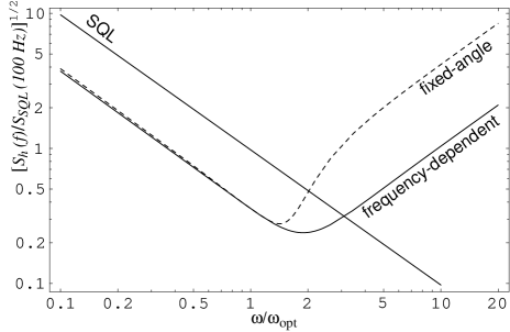
FIG. 10.: Comparison of typical noise curves for frequency-dependent and fixed-angle homodyne detection. The FD homodyne angle $\Phi(\omega)$ is that of Eqs. (82) and (83); the fixed homodyne angle $\Phi$ is that of Eq. (74); the circulating power is $e^{-2R}$ times that of Table I; and all other parameters are identical for the two interferometers and are given in Table I.

In the case of position-meter interferometers with optical filters (the interferometers analyzed by KLMTV), the optical losses due to the filter cavities contribute significantly to the noise spectral density and drastically reduce the ability to beat the SQL. It turns out that the squeezed-variational speed meter is less sensitive to such losses, as we shall see in Sec. V.

V Optical Losses

In order to understand the issue of optical losses in this speed meter, we shall start by addressing its internal losses. These include scattering and absorption at each optical element, finite transmissivities of the end mirrors, and imperfections of the mode-matching between cavities. The effect of external losses (i.e., losses in the detection system and any filter cavities) will be discussed separately. Note that the analysis in this section includes the internal and RSE mirrors, so it applies primarily to the speed meter designs in Figs. 3 and 4.

A Internal losses

In this subsection, we will consider only noise resulting from losses associated with optical elements inside the interferometer. These occur

• in the optical elements: arm cavities, sloshing cavity, extraction mirror, port-closing mirror, beam splitter, RSE mirror;

• due to mode-mismatching; and

• due to the imperfect matching of the transmissivities of the RSE and internal mirrors.

Since the optical losses will dominate, we focus only on that type of loss here. The loss at each optical element will decrease the amplitude of the sideband light (which carries the gravitational-wave information) and will simultaneously introduce additional vacuum fluctuations into the optical train. Schematically, for some sideband $\tilde{a}(\omega)$, the loss is described by

$$\tilde{a}(\omega)\rightarrow\sqrt{1-{\cal E}(\omega)}\,\tilde{a}(\omega)+\sqrt{{\cal E}(\omega)}\,\tilde{n}(\omega)\,,$$ (84)

where $\cal{E}$ is the (power) loss coefficient, and $\tilde{n}(\omega)$ is the vacuum field entering the optical train at the loss point.

It should be noted that there are various methods of grouping these losses together in order to simplify calculations. For example, we combine all of the losses occurring in the arm (or sloshing) cavities, into one loss coefficient of ${\cal L}\sim 20\times 10^{-6}$ [according to KLMTV Eq. (93)]. Then we assume that the end mirrors have transmissivity $T_{\rm e}=2\times 10^{-5}$, thereby absorbing all of the arm losses into one term [see KLMTV Eq. (B5) and preceding discussion].

Assuming that the noise entering at the end mirrors of the arm cavities is denoted $\tilde{n}_{e1,2}$ and $\tilde{n}_{n1,2}$ for the east and north arms respectively, at the end mirror of the sloshing cavity $\tilde{s}_{1,2}$, at the port-closing mirror $\widetilde{w}_{1,2}$, and at the RSE mirror $\widetilde{m}_{n1,2}$ and $\widetilde{m}_{s1,2}$ [representing the losses described in the previous paragraph; see Appendix B 3 for details], the output of the lossy three-cavity speed-meter system (Fig. 3; the simplified and practical versions are no longer equivalent, since there will be additional losses due to the presence of the internal and RSE mirrors) is

$$\tilde{q}_{1} = -{{\cal L}^{*}(\omega)\over{\cal L}(\omega)}\tilde{p}_{1}+\frac{i\omega\sqrt{\delta\delta_{\rm e}}}{{\cal L}(\omega)}(\tilde{n}_{e1}-\tilde{n}_{n1})+\frac{\Omega\sqrt{2\delta\delta_{\rm e}}}{{\cal L}(\omega)}\tilde{s}_{1}$$ (88)

$$\quad-\frac{\sqrt{T_{\rm e}}(\Omega^{2}-\omega^{2}+i\omega\delta_{\rm s})}{{\cal L}(\omega)}\widetilde{w}_{1}-\frac{i\omega\sqrt{2\delta\delta_{\epsilon}}}{{\cal L}(\omega)}\widetilde{m}_{s1}$$

$$\quad+\frac{\omega\sqrt{2L\delta\delta_{\epsilon}}(\omega-i\delta_{\rm i})}{\sqrt{c\delta_{\rm i}}{\cal L}(\omega)}\widetilde{m}_{n1}\,,$$

$$\tilde{q}_{2} = \frac{2i\omega\sqrt{\omega_{0}T_{\rm o}W_{\rm circ}^{\ast}}}{L\sqrt{\hbar}{\cal L}(\omega)}\tilde{x}-\frac{{\cal L}^{\ast}(\omega)}{{\cal L}(\omega)}\tilde{p}_{2}+\frac{\Omega\sqrt{2\delta\delta_{\rm e}}}{{\cal L}(\omega)}\tilde{s}_{2}$$ (91)

$$\quad+\frac{i\omega\sqrt{\delta\delta_{\rm e}}}{{\cal L}(\omega)}(\tilde{n}_{e2}-\tilde{n}_{n2})-\frac{\sqrt{T_{\rm e}}(\Omega^{2}-\omega^{2}+i\omega\delta_{\rm s})}{{\cal L}(\omega)}\widetilde{w}_{2}$$

$$\quad-\frac{i\omega\sqrt{2\delta\delta_{\epsilon}}}{{\cal L}(\omega)}\widetilde{m}_{s2}+\frac{\omega\sqrt{2L\delta\delta_{\epsilon}}(\omega-i\delta_{\rm i})}{\sqrt{c\delta_{\rm i}}{\cal L}(\omega)}\widetilde{m}_{n2}\,,$$

where

$$\tilde{x} = L\tilde{h}-\frac{4\sqrt{2\hbar\omega_{0}W_{\rm circ}^{\ast}}}{mc\omega^{2}{\cal L}(\omega)}\Biggl{[}\frac{i\omega\sqrt{2c\delta}}{\sqrt{L}}\tilde{p}_{1}+\frac{i\omega\sqrt{c\delta_{\epsilon}}}{\sqrt{L}}\widetilde{m}_{s1}$$ (94)

$$\quad\qquad\qquad-\frac{\sqrt{\delta_{\epsilon}}[\Omega^{2}-i\omega(\delta+\delta_{\rm i})]}{\sqrt{\delta_{\rm i}}}\widetilde{m}_{n1}-\frac{\Omega\sqrt{c\delta_{\rm e}}}{\sqrt{L}}\tilde{s}_{1}$$

$$\quad\qquad\qquad+i\omega\sqrt{\delta\delta_{\rm e}}\widetilde{w}_{1}-\frac{i\omega\sqrt{c\delta_{\rm e}}}{\sqrt{2L}}(\tilde{n}_{e1}-\tilde{n}_{n1})\Biggr{]}$$

with

$$\delta_{\rm e} =cT_{\rm e}/2L\,,\quad\delta_{\rm s} =cT_{\rm s}/2L\,,$$ (95)

$$\delta_{\rm i} =cT_{\rm i}/4L\,,\quad\delta_{\epsilon} =c{\cal E}/2L\,.$$ (96)

Note that the expression for the circulating power now has the form

$$W_{\rm circ}^{\ast}=\frac{1}{2}\hbar\omega_{0}B_{1}^{2}=\frac{4\hbar\omega_{0}T_{\rm i}T_{\rm p}I_{1}^{2}}{(T_{\rm i}T_{\rm p}+4T_{\rm e})^{2}}$$ (97)

[cf. Eq. (12)].

Equations (V A) are approximate expressions [accurate to about 6%, as were Eqs. (III A); see Footnote ¶ ‣ III A], where the assumptions (7) regarding the relative sizes of the transmissivities were used to simplify from the exact expressions. Alternatively, they can be derived analytically by keeping the leading order of the small quantities $\omega L/c\sim\sqrt{T_{\mathrm{s}}}\sim T_{\mathrm{o}}\sim T_{\mathrm{i}}$, plus the various loss factors; see Sec. VI of KLMTV and Sec. IV of Paper I for details of the derivations for other inteferometer designs. In addition to confirming the approximate formulas, such a derivation can also clarify the origins of various noise terms and their connections to one another.

B Internal and External Losses in Compact Form

In order to simplify the above Eqs. (V A) and (94), we define $\kappa^{*}$ in identically the same way as we defined $\kappa$ [Eq. (18) or (26)] but with $W_{\rm circ}\rightarrow W_{\rm circ}^{*}$. Let $\mathcal{E}^{\mathrm{S}}_{\mathcal{N}}$ and $\mathcal{E}^{\mathrm{R}}_{\mathcal{N}}$ represent the shot and radiation-pressure noises for the various parts of the interferometer, specified by $\cal N$. In Table II, expressions for $\mathcal{E}^{\mathrm{S}}_{\mathcal{N}}$ and $\mathcal{E}^{\mathrm{R}}_{\mathcal{N}}$ are given for $\cal N=$ AES (arm cavities, extraction mirror, and sloshing cavity combined), close (port-closing mirror), $\rm RSE_{in}$ (RSE cavity in the north direction, or going “in” to the arms), and $\rm RSE_{out}$ (RSE cavity in the south direction, or going “out” of the arms). The various $\varepsilon_{\cal N}$ represent the characteristic (and frequency-independent) fractional losses for each of these terms; values are given in Table III. Note that, by definition, $\mathcal{E}^{\mathrm{S}}_{\mathcal{N}}$ are required to be real, while $\mathcal{E}^{\mathrm{R}}_{\mathcal{N}}$ may have imaginary parts. For more information, including physical explanations of each of these terms, see Appendix B.

It is simple at this point to include the losses associated with optical elements external to the interferometer. These include losses are associated with

• the local oscillator used for homodyne detection,

• the inefficiency of the photodiode,

• the circulator by which the squeezed vacuum is injected, and

• the external filter cavities used for the variational-output scheme.

These can be addressed in the same manner as the losses inside the speed meter. We need only include two more terms in the summation, $\mathcal{N}=\mathrm{OPC}$ for the local oscillator, photodiode, and circulator and $\mathcal{N}=\mathrm{F}$ for the filters. Again, these terms are shown in Tables II and III and described in more detail in Appendix B.

TABLE II.: Loss factors $\cal E_{N}^{\rm S}$ due to shot noise and $\cal E_{N}^{\rm R}$ due to radiation pressure for each type of loss source in the interferometer.

Source	${\cal N}$		$\mathcal{E}^{\mathrm{S}}_{\cal N}$ (shot noise)		$\mathcal{E}^{\mathrm{R}}_{\cal N}$ (radiation pressure noise)
$\begin{array}[]{l}{\rm arm\ cavities,}\\ {\rm extract.\ mirror,}\\ {\rm sloshing\ cavity}\end{array}$	$\mathrm{AES}$		$\displaystyle\sqrt{\frac{\varepsilon_{\mathrm{AES}}}{T_{\mathrm{o}}}}\frac{\omega\delta}{|\mathcal{L}(\omega)|}$		$\displaystyle-\frac{e^{i\psi}}{2}\sqrt{\frac{\varepsilon_{\mathrm{AES}}}{{T}_{\rm o}}}$
$\begin{array}[]{l}{\rm\textrm{port-closing}}\\ {\rm mirror}\end{array}$	$\mathrm{close}$		$\displaystyle\sqrt{\varepsilon_{\mathrm{close}}}\,\frac{\Omega^{2}-\omega^{2}}{|\mathcal{L}(\omega)|}$		$\displaystyle-\frac{ie^{i\psi}}{2}\sqrt{\varepsilon_{\mathrm{close}}}$
$\begin{array}[]{l}{\rm RSE\ cavity}\\ {\rm``in"\ to\ arms}\end{array}$	$\mathrm{RSE}_{\mathrm{in}}$		$\displaystyle\sqrt{\frac{\varepsilon_{\mathrm{RSE}}T_{\mathrm{i}}}{4T_{\mathrm{o}}}\left(1+\frac{\omega^{2}}{\delta_{\mathrm{i}}^{2}}\right)}\frac{\omega\delta}{|\mathcal{L}(\omega)|}$		$\displaystyle e^{i\psi-i\beta_{\mathrm{i}}}\sqrt{\frac{\varepsilon_{\mathrm{RSE}}T_{\mathrm{o}}}{T_{\rm i}}}\frac{\omega(\delta_{\mathrm{i}}+\delta)+i\Omega^{2}}{\omega\delta}$
$\begin{array}[]{l}{\rm RSE\ cavity}\\ {\rm``out"\ to\ slosh}\end{array}$	$\mathrm{RSE}_{\mathrm{out}}$		$\displaystyle\sqrt{\frac{\varepsilon_{\mathrm{RSE}}T_{\mathrm{i}}}{4T_{\mathrm{o}}}\left(1+\frac{\omega^{2}}{\delta_{\mathrm{i}}^{2}}\right)}\frac{\omega\delta}{|\mathcal{L}(\omega)|}$		$\displaystyle e^{i\psi+i\beta_{\mathrm{i}}}\sqrt{\frac{\varepsilon_{\mathrm{RSE}}T_{\mathrm{o}}}{T_{\rm i}}}\frac{\omega(\delta_{\mathrm{i}}-\delta)-i\Omega^{2}}{\omega\delta}$
$\begin{array}[]{l}{\rm local\ oscillator,}\\ {\rm photodiode,}\\ {\rm and\ circulator}\end{array}$	OPC		$\displaystyle\sqrt{\varepsilon_{\rm OPC}}$		0
filter cavities	F		$\sqrt{\varepsilon_{\rm F}}$		0

TABLE III.: Fiducial values for the fractional losses occuring in various parts of the interferometer. These losses and their values are discussed in more detail in Appendix B.

Loss source	Symbol	Value
arm cavity	$\varepsilon_{\rm arm}$	$2\times 10^{-5}$
sloshing cavity	$\varepsilon_{\rm slosh}$	$2\times 10^{-5}$
extraction mirror	$\varepsilon_{\rm ext}$	$2\times 10^{-5}$
RSE cavity	$\varepsilon_{\rm RSE}$	$2\times 10^{-5}$
port-closing mirror	$\varepsilon_{\rm close}$	$2\times 10^{-5}$
local oscillator	$\varepsilon_{\rm lo}$	$0.001$
photodiode	$\varepsilon_{\rm pd}$	$0.001$
circulator	$\varepsilon_{\rm circ}$	$0.001$
mode-mismatch into filters	$\varepsilon_{\rm mm}$	$0.001$
Combined loss source terms
arms, extraction mirror, & sloshing cavitya	$\varepsilon_{\rm AES}$	$6\times 10^{-5}$
local oscillator, photodiode, & circulator	$\varepsilon_{\rm OPC}$	$0.003$
filter cavities (with mode mismatch)	$\varepsilon_{\rm F}$	$0.005$

Using these $\cal E_{N}^{\rm S}$ and $\cal E_{N}^{\rm R}$, we can rewrite the input-output relation (V A) in the same form as Eq. (III A) as follows:

$$\left(\begin{array}[]{c}\tilde{q}_{1}\\ \tilde{q}_{2}\end{array}\right) = e^{2i\psi}\left(\begin{array}[]{cc}1&0\\ -\kappa^{*}&1\end{array}\right)\left(\begin{array}[]{c}\tilde{p}_{1}\\ \tilde{p}_{2}\end{array}\right)$$ (112)

$$\quad+\sum_{\mathcal{N}}e^{2i\alpha_{\mathcal{N}}}\left(\begin{array}[]{rr}\mathcal{E}^{S}_{\mathcal{N}}&0\\ -\kappa^{*}\mathcal{E}^{\mathrm{R}}_{\mathcal{N}}&\mathcal{E}^{S}_{\mathcal{N}}\end{array}\right)\left(\begin{array}[]{c}n_{{\cal N}1}\\ n_{{\cal N}2}\end{array}\right)$$

$$\quad+\sqrt{2\kappa^{*}}\frac{h}{h_{{SQL}}}e^{i\psi}\left(\begin{array}[]{c}0\\ 1\end{array}\right)\,,$$

where the $\alpha_{\mathcal{N}}$ are uninteresting phases that do not affect the noise.

The relative magnitudes of the loss terms are shown in Fig. 11. From the plot, we can see that there are several loss terms—specifically, the shot noise from the AES, OPC, and filter cavities (if any)—that are of comparable magnitude at high frequencies and dominate there. The AES radiation-pressure term dominates at low frequencies, and the RSE radiation-pressure terms are also significant. Since the largest noise sources at low frequencies are radiation-pressure terms, they will be dependent on the circulating power. Consequently, those terms will become smaller when the circulating power is reduced, as when squeezed vacuum is injected into the dark port. This will be demonstrated in Fig. 12 below.

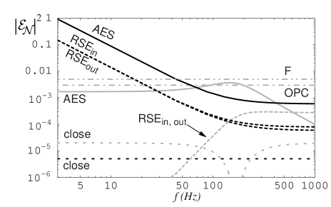
FIG. 11.: Moduli-squared of the loss factors shown in Table II. In general, the black curves are the radiation-pressure noise and the gray curves are the shot noise. The parameters used for this plot are given in Tables I and III.

To compute the spectral noise density, we suppose the output at homodyne angle $\Phi$ is measured, giving

$$S_{h_{n}}(\omega) = \frac{(h_{{SQL}})^{2}}{2\kappa^{*}}\Biggl{\{}\bigg{[}(\cot\Phi-\kappa^{*})^{2}+1\bigg{]}$$ (114)

$$\quad+\sum_{\mathcal{N}}\bigg{[}|{\cal E}^{\mathrm{S}}_{\mathcal{N}}\cot\Phi-{\cal E}^{\mathrm{R}}_{\mathcal{N}}\kappa^{*}|^{2}+({\cal E}^{\mathrm{S}}_{\mathcal{N}})^{2}\bigg{]}\Biggr{\}}\,,$$

where we have assumed all of the vacuum fluctuation spectral densities are unity and the cross-correlations are zero; this is the same technique that we used to derive Eqs. (22) and (80) and that was used in Paper I and KLMTV. Given the complicated behaviors of $\mathcal{E}^{\mathrm{S}}_{\cal N}$ and $\mathcal{E}^{\mathrm{R}}_{\cal N}$, including these loss terms in the optimization of the homodyne phase $\Phi(\omega)$ is unlikely to be helpful. Therefore, we will use $\cot\Phi=\kappa_{\mathrm{max}}^{*}$, as in the lossless case. This gives us a total noise with losses:

$$S_{h_{n}}(\omega) = \frac{(h_{{SQL}})^{2}}{2\kappa^{*}}\Biggl{\{}\bigg{[}(\kappa_{\mathrm{max}}^{*}-\kappa^{*})^{2}+1\bigg{]}$$ (116)

$$\quad+\sum_{\mathcal{N}}\bigg{[}|{\cal E}^{\mathrm{S}}_{\mathcal{N}}\kappa^{*}_{\mathrm{max}}-{\cal E}^{\mathrm{R}}_{\mathcal{N}}\kappa^{*}|^{2}+({\cal E}^{\mathrm{S}}_{\mathcal{N}})^{2}\bigg{]}\Biggr{\}}\,.$$

When we inject squeezed vacuum into the dark port, we get output operators

$$\left(\begin{array}[]{c}\tilde{q}_{1s}\\ \tilde{q}_{2s}\end{array}\right) = e^{2i\psi}\left(\begin{array}[]{cc}1&0\\ -\kappa^{*}&1\end{array}\right)\left(\begin{array}[]{c}e^{R}\tilde{p}_{1}\\ e^{-R}\tilde{p}_{2}\end{array}\right)$$ (131)

$$\quad+\sum_{\mathcal{N}}e^{2i\alpha_{\mathcal{N}}}\left(\begin{array}[]{rr}\mathcal{E}^{S}_{\mathcal{N}}&0\\ -\kappa^{*}\mathcal{E}^{\mathrm{R}}_{\mathcal{N}}&\mathcal{E}^{S}_{\mathcal{N}}\end{array}\right)\left(\begin{array}[]{c}n_{{\cal N}1}\\ n_{{\cal N}2}\end{array}\right)$$

$$\quad+\sqrt{2\kappa^{*}}\frac{h}{h_{{SQL}}}e^{i\psi}\left(\begin{array}[]{c}0\\ 1\end{array}\right)$$

that can be regarded as acting on the ordinary vacuum states of the input. Once again assuming that the vacuum fluctuation spectral densities are unity and the cross-correlations are zero, the squeezed-input noise spectral density with homodyne detection at phase $\Phi$ is

$$S_{h_{ns}}(\omega) = \frac{(h_{{SQL}})^{2}}{2\kappa^{*}}\Biggl{\{}\bigg{[}(\cot\Phi-\kappa^{*})^{2}e^{2R}+e^{-2R}\bigg{]}$$ (133)

$$\ +\sum_{\mathcal{N}}\bigg{[}|{\cal E}^{\mathrm{S}}_{\mathcal{N}}\cot\Phi-{\cal E}^{\mathrm{R}}_{\mathcal{N}}\kappa^{*}|^{2}+({\cal E}^{\mathrm{S}}_{\mathcal{N}})^{2}\bigg{]}\Biggr{\}}\,.$$

C Performance of Lossy Speed Meters and Comparisons with Other Configurations

Examples of lossy speed meter noise curves with and without squeezed vacuum [Eqs. (116) and (133)] are shown in Fig. 12. Note that, as mentioned before, the losses are less significant when squeezed vacuum is used to reduce the circulating power, since the radiation-pressure noise coming from the losses is reduced. In the ordinary speed meter (no squeezed vacuum), the losses increase $\sqrt{S_{h_{n}}}$ by $5-9\%$ in the band $50-105~{}\rm Hz$. The losses have little effect above this range, but below it, noise increases significantly, mostly due to the radiation-pressure noises shown in Fig. 11. For the squeezed-input speed meter (power squeeze-factor $e^{-2R}=0.1$), the losses increase $\sqrt{S_{h_{n}}}$ by $3-4\%$ in the band $25-150~{}\rm Hz$. Again, the losses have little effect above this range. At low frequencies, however, the losses get quite large: $11\%$ at 10 Hz, $32\%$ at 5 Hz, and $73\%$ at 3 Hz. Losses in the squeezed-variational speed meter are much the same as in the squeezed-input speed meter. The slight difference at low frequencies is due to the fact that the lossless squeezed-variational speed meter is slightly better in that regime than the ordinary or squeezed-input speed meter.

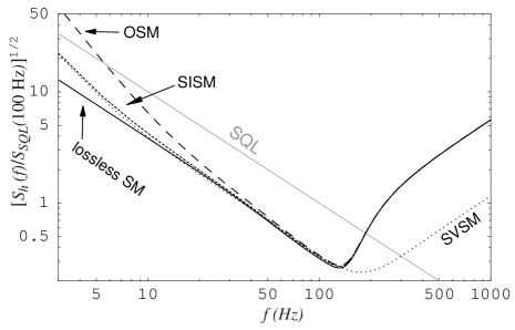
FIG. 12.: Noise curves showing the effects of losses. Noise curves for lossy versions of the ordinary (OSM), squeezed-input (SISM), and squeezed-variational (SVSM) speed meters are shown, along with a curve of the lossless ordinary speed meter for comparison. All speed meter curves here have the same parameters: $\delta=2\omega_{\rm opt}$, $\Omega=\sqrt{3}\omega_{\rm opt}$, $\omega_{\rm opt}=2\pi\times 100~{}\rm Hz$, and $T_{\rm i}=0.005$. The rest of the parameters are given in Tables I and III.

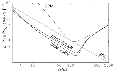
FIG. 13.: Comparison of noise curves of a conventional position meter (CPM) and squeezed-input speed meters (SISM) with circulating powers $W_{\rm circ}=820~{}\rm kW$ and $W_{\rm circ}=2~{}\rm MW$. The speed meters have $f_{\rm opt}=107~{}\rm Hz$, with $\Omega$ and $\delta$ determined by Eq. (33). Other parameters used are those in Tables I and III with $T_{\rm i}=0.005$ and $e^{-2R}=0.1$.

The noise curves of squeezed-input speed meters (with ordinary homodyne detection) compared with the SQL are shown in Fig. 13, along with the noise of a conventional position meter with the same optical power. These speed meters beat the SQL in a broad frequency band, despite the losses. In particular, the noise curve for the speed meter with $W_{\rm circ}=800\,{\rm kW}$ (and $f_{\rm opt}=107\,{\rm Hz}$) matches the curve of the conventional position meter at high frequencies, while it beats the SQL by a factor of $\sim 8$ (in power) below $\sim 150\,{\rm Hz}$. In terms of the signal-to-noise ratio for neutron star binaries, for example, this configuration improves upon the conventional design by a factor of $3.6$ in signal-to-noise ratio, which corresponds to a factor of $43$ increase in event rate. If it is possible to have a higher circulating power, say $W_{\rm circ}=2\,{\rm MW}$, the squeezed-input speed meter would be able to beat the SQL by a factor of $\sim 14$, corresponding to a factor of 4.6 in signal-to-noise and 97 in event rate. (Such a noise curve is shown in Fig. 13).

The broadband behaviors of the speed meters with losses are particularly interesting. We start by looking at the expression for the noise spectral density, Eq. (133). An ideal (lossless) speed meter in the broadband configuration beats the SQL from 0 Hz up to $\omega\sim\omega_{\rm opt}$, by roughly a constant factor, because $\kappa$ is roughly constant in this band. This is the essential feature of the speed meter; see Sec. III. Focusing on this region, we have, approximately (for squeezed-input speed meters that are lossy):

$$S_{h_{ns}}(\omega) \approx \frac{h_{SQL}^{2}}{2\kappa^{*}_{\rm max}}\biggl{[}e^{-2R}+\sum_{\cal N}|{\cal E}_{\cal N}^{S}|^{2}$$ (135)

$$\qquad\qquad+{\kappa^{*}}_{\rm max}^{2}\sum_{\cal N}|{\cal E}_{\cal N}^{\rm S}-{\cal E}_{\cal N}^{\rm R}|^{2}\biggr{]}\,.$$

Qualitatively, we can see that if the losses are not severe or if $\kappa^{*}_{\rm max}$ is relatively small (such that the later two terms in the above equation are small compared to the power squeeze factor $e^{-2R}$), the losses do not contribute significantly to the total noise. If, in addition, the dominant loss factors are (almost) frequency independent, then the noise due to losses gives a rather constant contribution, as shown by curves in Fig. 12. In particular, the large bandwidth is preserved. (There is a slight exception to this statement in the absence of squeezed input. Without squeezed input, the circulating power is higher, causing $\kappa^{*}_{\rm max}$ to be $10$ times larger than the other cases. Consequently, the frequency dependence of ${\cal E}_{\rm AES}^{\rm R}$ to appear in the output.)

As $\kappa_{\rm max}$ increases, the noise from the losses may become dominant. In fact, when one minimizes the noise spectral density with respect to $\kappa^{*}_{\rm max}$, one obtains the following loss-dominated result:

$$S^{\rm L}_{h}(\omega)\approx h_{SQL}^{2}\sqrt{\left(\sum_{\cal N}|{\cal E}_{\cal N}^{\rm S}-{\cal E}_{\cal N}^{\rm R}|^{2}\right)\left(e^{-2R}+\sum_{\cal N}|{\cal E}_{\cal N}^{\rm S}|^{2}\right)}\,,$$ (136)

which is achieved if and only if

$$\kappa^{*}_{\rm max}=\kappa^{\rm L}\equiv\sqrt{\frac{e^{-2R}+\sum_{\cal N}|{\cal E}_{\cal N}^{\rm S}|^{2}}{\sum_{\cal N}|{\cal E}_{\cal N}^{\rm S}-{\cal E}_{\cal N}^{\rm R}|^{2}}}\,.$$ (137)

This $\kappa^{\rm L}$ is rather constant and is comparable in magnitude to the values of $\kappa^{*}(\omega)$ of our speed meters, suggesting that the speed meters can become loss-limited over a broad band of frequencies. Contrast this with the KLMTV position meters, where ${\cal K}_{*}(\omega)$ grows as $\omega^{-2}$ at low frequencies; see Fig. 14. This is a fundmental property of displacement meters. As a result, a position meter optimized at some frequency $f_{\rm opt}$ may be able to reach its “loss limit” (the equivalent of $S_{h}^{\rm L}$) at that frequency $f_{\rm opt}$, but doing so will result in a sharp growth of noise at freqencies below $f_{\rm opt}$. In contrast, a speed meter similarly optimized is able to stay at the noise level of its loss limit $S_{h}^{\rm L}$ over a wide band of frequencies below $f_{\rm opt}$; see Fig. 15. While it is unfortunate that losses limit the performance of interferometers, the speed meter is at least able to retain a wide-band sensitivity even in the presence of a loss-limit.

To give a specific example of this loss-limit phenomenon, we first notice that, with the same circulating power, the conventional position-meter ${\cal K}_{*}$ and our (squeezed-variational) speed-meter $\kappa$ agree if $\delta=\gamma$ (where $\gamma$ is the bandwidth of the arm cavities, as defined in KLMTV) and if we consider high frequencies ($\omega\gtrsim\{\gamma,\,\Omega\}$). Figure 14 shows an example of this [with $W_{\rm circ}=820\,{\rm kW}$, $\gamma=\delta=2\pi\times 100\,{\rm Hz}$, $\Omega=2\pi\times 173\,{\rm Hz}$]. The noise curves of the two interferometers are shown in Fig. 15.

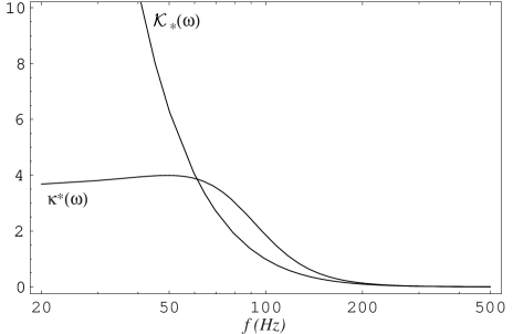
FIG. 14.: Comparison of the squeezed-variational speed meter’s $\kappa^{*}$ with the equivalent coupling constant $\cal K_{*}$ (as defined by KLMTV) for the squeezed-variational position meter. Parameters are $W_{\rm circ}=820\,{\rm kW}$, $\gamma=\delta=2\pi\times 100\,{\rm Hz}$, $\Omega=2\pi\times 173\,{\rm Hz}$.

As expected, the two noise curves in Fig. 15 agree at very high frequencies. At intermediate frequencies, the speed meter’s $\kappa^{*}$ is larger than the position meter’s ${\cal K}_{*}$, and thus the speed meter has better sensitivity than the position meter. As the frequency decreases, the speed meter reaches its loss limit first and stays at that limit for a wide range of frequencies. The position meter, however, only touches its loss limit and then increases rapidly.

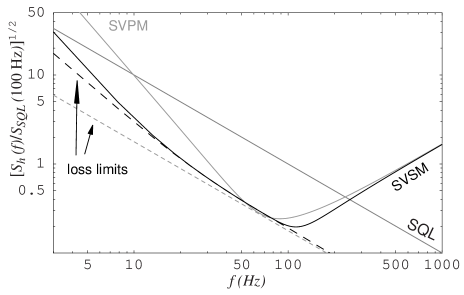
FIG. 15.: Comparison of noise curves for a squeezed-variational position meter (SVPM; analyzed in KLMTV) and for a squeezed-variational speed meter (SVSM; analyzed in this paper). Parameters used are those in Tables I and III with $T_{\rm i}=0.005$ and $e^{-2R}=0.1$. Also shown are the loss limits described in Sec. V C.

VI Conclusions

We have described and analyzed a speed-meter interferometer that has the same performance as the two-cavity design analyzed in Paper I, but it does so without the substantial amount of power flowing through the system or the exorbitantly high input laser power required by the two-cavity speed meter. It was also shown that the injection of squeezed vacuum with $e^{-2R}=0.1$ into the dark port of the interferometer will reduce the needed circulating power by an order of magnitude, bringing it into a range that is comparable to the expected circulating power of LIGO-II, if one wishes to beat the SQL by a factor of $\sqrt{10}$ in amplitude. Additional improvements to the sensitivity, particularly at high frequencies, can be achieved through the use of frequency-dependent homodyne detection.

In addition, it was shown that this type of speed-meter interferometer is not nearly as susceptible to losses as those presented in KLMTV. Its robust performance is due, in part, to the functional form the coupling factor $\kappa$, which is roughly constant at low frequencies. This helps to maintain the speed meters’ wideband performance, even in the presence of losses. Losses for the various speed meters we discuss here are generally quite low. The dominant sources of loss-induced noise at low frequencies ($f\lesssim f_{\rm opt}$) are the radiation-pressure noise from losses in the arm, extraction, and sloshing cavities. Because this type of noise is dependent on the circulating power, it can be reduced by reducing the power by means of squeezed input.

A FP Cavities as Optical Filters

As proposed by KLMTV [Sec. V B and Appendix C], Fabry-Perot cavities can be used as optical filters to achieve frequency-dependent homodyne detection. Here we shall briefly summarize and generalize their results.

Suppose we have one FP cavity of length $L_{\rm FP}$ and resonant frequency $\omega_{0}-\xi_{\rm FP}\delta_{\rm FP}$. Also suppose this cavity has an input mirror with finite transmissivity $T_{\rm FP}$ and a perfect end mirror. When sideband fields at frequency $\omega_{0}\pm\omega$ emerge from the cavity, they have a phase shift

$$\alpha_{\pm}\equiv 2\arctan(\xi_{\rm FP}\pm\omega/\delta_{\rm FP})\;,$$ (A1)

where

$$\delta_{\rm FP}=\frac{cT_{\rm FP}}{4L_{\rm FP}}$$ (A2)

is the half bandwidth of the cavity. [Note that Eq. (A1) is KLMTV Eqs. (88) and (C2), but a factor of 2 was missing from their equations. Fortunately, this appears to be a typographical error only in that particular equation; the factor of 2 is included in their subsequent calculations.] As a result of this phase shift, the input ($\tilde{b}_{1,2}$)–output (${b}_{1,2}$) relation for sideband quadratures at frequency $\omega$ will be [KLMTV Eqs. (78)]

$$\left(\begin{array}[]{c}\tilde{b}_{1}\\ \tilde{b}_{2}\end{array}\right)=e^{i\,\alpha_{\rm m}}\,{\bf R}_{\alpha_{\rm p}}\left(\begin{array}[]{c}b_{1}\\ b_{2}\end{array}\right)\,,$$ (A3)

where

$$\alpha_{\rm m}\equiv\frac{1}{2}(\alpha_{+}-\alpha_{-})\,,\quad\alpha_{\rm p}\equiv\frac{1}{2}(\alpha_{+}+\alpha_{-})\,,$$ (A4)

and

$${\bf R}_{\phi}\equiv\left(\begin{array}[]{rr}\cos\phi&-\sin\phi\\ \sin\phi&\cos\phi\end{array}\right)\,.$$ (A5)

If a frequency-independent homodyne detection at phase shift $\theta$ follows the optical filter, the measured quantity will be [KLMTV Eqs. (81) and (82)]

$$\tilde{b}_{\theta}=e^{i\alpha_{\rm m}}b_{\zeta}\,,$$ (A6)

where

$$\zeta(\omega)=\theta-\alpha_{\rm p}\equiv\theta-\frac{1}{2}(\alpha_{+}+\alpha_{-})\,.$$ (A7)

If more than one filter is applied in sequence (I, II, …,) and followed by homodyne detection at angle $\theta$, the measured quadrature will be [Eq. (83)]

$$\zeta(\omega)=\theta-\frac{1}{2}(\alpha_{\rm I+}+\alpha_{\rm I-}+\alpha_{\rm II+}+\alpha_{\rm II-}+\ldots)\,.$$ (A8)

[Note that this $\zeta(\omega)$ (KLMTV’s notation) is the same homodyne angle $\Phi(\omega)$ that we want to produce.] By adjusting the parameters $\xi_{J}$ and $\delta_{J}$, one might be able to achieve the FD homodyne phases needed. KLMTV worked out a particular case for their design [their Sec. V B, V C, and Appendix C].

Here we shall seek a more complete solution that works in a large class of situations. With the help of Eq. (A1), Eq. (A8) can be written in an equivalent form

$$\frac{1+i\tan\zeta}{1-i\tan\zeta} = e^{2i\theta}\prod_{J={\rm I},{\rm II},\ldots\,,s=\pm}\frac{1-i\tan\left(\alpha_{Js}/2\right)}{1+i\tan\left(\alpha_{Js}/2\right)}\,,$$ (A9)

$$= e^{2i\theta}\prod_{J={\rm I},{\rm II},\ldots\,,s=\pm}\frac{\omega-s(-\xi_{J}\delta_{J}-i\delta_{J})}{\omega-s(-\xi_{J}\delta_{J}+i\delta_{J})}\,.$$ (A10)

Suppose the required $\tan\zeta(\omega)$ is a rational function in $\omega^{2}$,

$$\tan\zeta(\omega)=\frac{\sum_{k=0}^{n}B_{k}\omega^{2k}}{\sum_{k=0}^{n}A_{k}\omega^{2k}}\,,$$ (A11)

where $A_{k}$ and $B_{k}$ are real constants with $A_{n}^{2}+B_{n}^{2}>0$. Then Eq. (A9) requires that, for all $\omega$,

$$\sum_{k=0}^{n}(A_{k}+iB_{k})\omega^{2k}$$ (A12)

$$\quad=D\,e^{i\theta}\prod_{J={\rm I},{\rm II},\ldots\,,s=\pm}\bigg{[}{\omega-s(-\xi_{J}\delta_{J}-i\delta_{J})}\bigg{]}\,,$$ (A13)

where $D$ can be any real constant. Equation (A12) can be solved as follows. First, match the roots of the polynomials of $\omega$ on the two sides of the equation; denote these roots by $\pm\omega_{\rm J}$ with $J=1,2,\ldots,n$. Then we can deduce that $n$ filters are needed, and their complex resonant frequencies must be offset from $\omega_{0}$ by

$$\omega_{J}=-\delta_{J}\xi_{J}-i\delta_{J}\,,\quad J={\rm I},{\rm II},\ldots\,,$$ (A14)

where $\pm\omega_{\rm I,II,\ldots}$ [with $\Im(\omega_{J})>0$] are the $2n$ roots of

$$\sum_{k=0}^{n}(A_{k}+iB_{k})\,\omega^{2k}\,.$$ (A15)

After this, the polynomials on the two sides of Eq. (A12) can only differ by a complex coefficient whose argument determines $\theta$. In fact, by comparing the coefficients of $\omega^{2n}$ on both sides, we have

$$\theta=\arg(A_{2n}+iB_{2n})\,.$$ (A16)

B Semi-Analytical Treatment of the Loss Terms

In this appendix, we present a semi-analytic treatment of each source of noise included in Sec. V A. We will use a notation similar to Eq. (III A), but in matrix form:

$$\left(\begin{array}[]{c}\tilde{q}_{1}\\ \tilde{q}_{2}\end{array}\right)=\left(\begin{array}[]{c}\tilde{q}_{1}\\ \tilde{q}_{2}\end{array}\right)_{\rm lossless}+{\mathbf{N}_{\rm loss\ source}}\;,$$ (B1)

where ${\mathbf{N}_{\rm loss\ source}}$ is a vectorial representation of whichever source of loss we are considering at the moment. Each of these terms is associated with a vacuum field of the form $\sqrt{\cal E(\omega)}\tilde{n}(\omega)$ [cf. Eq. (84)], which enters the interferometer and increases the level of noise present. For generality, we let $\cal E(\omega)$ be frequency dependent. The (constant) characteristic fractional losses for each type of loss will be denoted by $\varepsilon$ with an appropriate subscript. Each loss term appearing in Table II is presented in a subsection below.

1 Arms, Extraction Mirror, and Sloshing Cavity (AES)

The losses in the arms allow an unsqueezed vacuum field $\sqrt{\varepsilon_{\mathrm{arm}}}\tilde{n}_{\mathrm{arm}}$ to enter the optical train. By idealizing this field as arising entirely at the arm’s end mirror, propagating the field through the interferometer to the output port, we obtain the following contribution to the output [cf. Eq. (84)]. The associated noise can be put into the following form

$${\mathbf{N}}_{\mathrm{arm}} = -\sqrt{\frac{\varepsilon_{\mathrm{arm}}}{T_{\mathrm{o}}}}\,\Biggl{[}e^{i\psi}\frac{\omega\delta}{|\mathcal{L}(\omega)|}\left(\begin{array}[]{cc}1&0\\ 0&1\end{array}\right)$$ (B9)

$$\qquad+e^{2i\psi}\left(\begin{array}[]{cc}0&0\\ \kappa^{*}/2&0\end{array}\right)\Biggr{]}\left(\begin{array}[]{c}\tilde{n}_{\mathrm{arm}1}\\ \tilde{n}_{\mathrm{arm}2}\end{array}\right)\,,$$

where the vacuum operators from the two arms are combined as

$$\tilde{n}_{\rm arm}j=\frac{\tilde{n}_{ej}-\tilde{n}_{nj}}{\sqrt{2}}\;.$$ (B10)

The first term (independent of $\kappa^{*}$) is the shot-noise contribution, while the second term (proportional to $\kappa^{*}$) is the radiation-pressure noise. It turns out that several of the other loss sources $\cal N$ have a similar mathematical form.

We consider, specifically, the loss from the extraction mirror, which effectively allows $\sqrt{\varepsilon_{\mathrm{ext}}}\,\tilde{n}_{\mathrm{ext}}$ into the optical train. By propagating this field through the interferometer to the output port, we obtain the following contribution to the noise:

$${\mathbf{N}}_{\mathrm{ext}} = \sqrt{\frac{\varepsilon_{\mathrm{ext}}}{T_{\mathrm{o}}}}\,\Biggl{[}e^{i\psi}\frac{\omega\delta}{|\mathcal{L}(\omega)|}\left(\begin{array}[]{cc}1&0\\ 0&1\end{array}\right)$$ (B18)

$$\qquad\qquad+e^{2i\psi}\left(\begin{array}[]{cc}0&0\\ \kappa^{*}/2&0\end{array}\right)\Biggr{]}\left(\begin{array}[]{c}\tilde{n}_{\mathrm{ext}1}\\ \tilde{n}_{\mathrm{ext}2}\end{array}\right)\,.$$

The loss from the sloshing cavity is a bit different: the imperfect end mirror of the sloshing cavity produces a vacuum noise field $\sqrt{\varepsilon_{\mathrm{slosh}}}\,\tilde{n}_{\mathrm{slosh}}$ which exits the cavity with the form

$$\sqrt{\frac{4\varepsilon_{\mathrm{slosh}}/T_{\mathrm{s}}}{1+\omega^{2}/(\delta_{\mathrm{s}}/2)^{2}}}e^{i\beta_{\mathrm{s}}}\tilde{n}_{\mathrm{slosh}\,1,2}\approx\sqrt{\varepsilon_{\mathrm{slosh}}}\frac{i\Omega}{\omega}\tilde{n}_{\mathrm{slosh}\,1,2}\,,$$ (B19)

where $\beta_{\mathrm{s}}\equiv\arctan(2\omega/\delta_{s})\approx\pi/2$ for most of the frequency band of interest. The associated noise is

$${\mathbf{N}}_{\mathrm{slosh}} = -\sqrt{\frac{\varepsilon_{\mathrm{slosh}}}{T_{\mathrm{o}}}}\frac{i\Omega}{\omega}\,\Biggl{[}e^{i\psi}\frac{\omega\delta}{|\mathcal{L}(\omega)|}\left(\begin{array}[]{cc}1&0\\ 0&1\end{array}\right)$$ (B27)

$$\qquad\qquad+e^{2i\psi}\left(\begin{array}[]{cc}0&0\\ \kappa^{*}/2&0\end{array}\right)\Biggr{]}\left(\begin{array}[]{c}\tilde{n}_{\mathrm{slosh}1}\\ \tilde{n}_{\mathrm{slosh}2}\end{array}\right)\,.$$

Since the vacuum fields $\tilde{n}_{\mathrm{arm}}$, $\tilde{n}_{\mathrm{ext}}$, and $\tilde{n}_{\mathrm{slosh}}$ are independent and uncorrelated, we can effectively combine these four noises into a single expression

$${\mathbf{N}}_{\mathrm{AES}} = \sqrt{\frac{\varepsilon_{\mathrm{AES}}}{T_{\mathrm{o}}}}\,\Biggl{[}e^{i\psi}\frac{\omega\delta}{|\mathcal{L}(\omega)|}\left(\begin{array}[]{cc}1&0\\ 0&1\end{array}\right)$$ (B35)

$$\qquad\qquad+e^{2i\psi}\left(\begin{array}[]{cc}0&0\\ \kappa^{*}/2&0\end{array}\right)\Biggr{]}\left(\begin{array}[]{c}\tilde{n}_{\mathrm{AES}1}\\ \tilde{n}_{\mathrm{AES}2}\end{array}\right)\,,$$

with

$$\varepsilon_{\mathrm{AES}}\sim{\cal E}_{\rm AES}(\omega)\equiv\varepsilon_{\mathrm{arm}}+\varepsilon_{\mathrm{ext}}+\varepsilon_{\mathrm{slosh}}\Omega^{2}/\omega^{2}\;.$$ (B36)

We expect that $\varepsilon_{\rm arm}\sim\varepsilon_{\rm slosh}\sim\varepsilon_{\rm ext}\sim 2\times 10^{-5}$, as discussed in the paragraph following Eq. (84) and as shown in Table III.

2 Port-Closing Mirror

The imperfection of the closing mirror has two effects: (i) it introduces directly a fluctuation $-\sqrt{\varepsilon_{\mathrm{close}}R_{\mathrm{o}}}\,\tilde{n}_{\mathrm{close}}$ into the output, giving a shot noise

$${\mathbf{N}}^{\mathrm{shot}\,\mathrm{direct}}_{\mathrm{close}}=-\sqrt{\varepsilon_{\mathrm{close}}R_{\mathrm{o}}}\left(\begin{array}[]{c}\tilde{n}_{\mathrm{close}1}\\ \tilde{n}_{\mathrm{close}2}\end{array}\right)\,;$$ (B37)

and (ii) it introduces a fluctuation $\sqrt{\varepsilon_{\mathrm{close}}T_{\mathrm{o}}}\,\tilde{n}_{\mathrm{close}}$ into the light that passes from the arms into the sloshing cavity, giving (after propagation through the sloshing cavity and interferometer and into the output):

$${\mathbf{N}}^{\mathrm{indirect}}_{\mathrm{close}} = -\sqrt{\varepsilon_{\mathrm{close}}}\,\Biggl{[}e^{i\psi}\frac{\omega\delta}{|\mathcal{L}(\omega)|}\left(\begin{array}[]{cc}1&0\\ 0&1\end{array}\right)$$ (B45)

$$\qquad\quad+e^{2i\psi}\left(\begin{array}[]{cc}0&0\\ \kappa^{*}/2&0\end{array}\right)\Biggr{]}\left(\begin{array}[]{c}\tilde{n}_{\mathrm{close}1}\\ \tilde{n}_{\mathrm{close}2}\end{array}\right)\,.$$

Combining these two expressions gives, to leading order (in the various transmissivities and the small parameters $\omega L/c$ and $\varepsilon_{\rm close}$),

$${\mathbf{N}}_{\mathrm{close}} = \sqrt{\varepsilon_{\mathrm{close}}}\,\Biggl{[}ie^{i\psi}\frac{\Omega^{2}-\omega^{2}}{|\mathcal{L}(\omega)|}\left(\begin{array}[]{cc}1&0\\ 0&1\end{array}\right)$$ (B53)

$$\qquad\quad-e^{2i\psi}\left(\begin{array}[]{cc}0&0\\ \kappa^{*}/2&0\end{array}\right)\Biggr{]}\left(\begin{array}[]{c}\tilde{n}_{\mathrm{close}1}\\ \tilde{n}_{\mathrm{close}2}\end{array}\right)\,.$$

Since $\varepsilon_{\rm close}$ is simply the loss from the port-closing mirror itself, we can assume that $\varepsilon_{\rm close}\lesssim 2\times 10^{-5}$. Then, this and the above expression (B53) show that the output noise from the closing mirror is $T_{\mathrm{o}}$ times smaller than the AES loss [Eq. (B36)].

3 The RSE Cavity

The losses in the region between the internal mirrors and the RSE mirror, i.e., the RSE cavity, are more complicated than the previous cases. As before, we suppose that, during each propagation from one end to the other of the RSE cavity, a fraction $\varepsilon_{\mathrm{RSE}}$ of the light power is dissipated and replaced by a corresponding vacuum field, $\sqrt{\varepsilon_{\rm RSE}}\,\tilde{n}_{\mathrm{in}}$ or $\sqrt{\varepsilon_{\rm RSE}}\,\tilde{n}_{\mathrm{out}}$ (depending whether the light is propagating in towards the arms or out towards the extraction mirror and sloshing cavity). These two fields $\tilde{n}_{\mathrm{in}}$ and $\tilde{n}_{\mathrm{out}}$ are independent vacuum fields. At the leading order in $\varepsilon_{\mathrm{RSE}}$, we have a modified version of the “input–output” relation for the RSE cavity:

$$\left(\begin{array}[]{c}B\\ D\end{array}\right) = \left(\begin{array}[]{cc}1-\frac{1+R_{\mathrm{i}}}{2T_{\mathrm{i}}}\varepsilon_{\mathrm{RSE}}&\frac{\sqrt{R_{\mathrm{i}}}}{\mathrm{T}_{\mathrm{i}}}\varepsilon_{\mathrm{RSE}}\\ \frac{\sqrt{R_{\mathrm{i}}}}{\mathrm{T}_{\mathrm{i}}}\varepsilon_{\mathrm{RSE}}&1-\frac{1+R_{\mathrm{i}}}{2T_{\mathrm{i}}}\varepsilon_{\mathrm{RSE}}\end{array}\right)\left(\begin{array}[]{c}A\\ C\end{array}\right)$$ (B65)

$$\,+\sqrt{\frac{\varepsilon_{\mathrm{RSE}}}{T_{\mathrm{i}}}}\left(\begin{array}[]{cc}1&-\sqrt{R_{\mathrm{i}}}\\ -\sqrt{R_{\mathrm{i}}}&1\end{array}\right)\left(\begin{array}[]{c}\tilde{n}_{\mathrm{in}}\\ \tilde{n}_{\mathrm{out}}\end{array}\right)\,,$$

where $A,B,C,D$ are the field amplitudes shown in Fig. 3. Note that, for simplicity, we are looking at only one arm; we could equally well use the other (substituting $B\rightarrow F$ and $C\rightarrow G$) or the proper combination of both. Also, notice that if $\varepsilon_{\mathrm{RSE}}=0$, then we find $B=A$ and $D=C$, which illustrates the fact that the internal and RSE mirrors have no effect on the sidebands (described in Sec. I where we introduced the RSE mirror).

From Eq. (B65), we find that the loss inside the RSE cavity has two effects. First, it makes the cancellation of the effect of the internal and the RSE mirrors imperfect. (Recall that an RSE mirror with the same transmissivity as the internal mirrors effectively cancels the effect of the internal mirrors on the sidebands; this was discussed in Sec. I.) This imperfect cancellation will not be important in our situation. Indeed, there is no corresponding term appearing in the input–output relation given in Eq. (V A).

Secondly, the loss inside the RSE cavity adds two vacuum fields to light that travels through the RSE cavity in opposite directions [i.e., from A to B (IN) and from C to D (OUT)]. We denote them by

$$\tilde{\mathfrak{N}}_{\mathrm{IN}} \equiv \sqrt{\frac{\varepsilon_{\mathrm{RSE}}}{T_{\mathrm{i}}}}(\tilde{n}_{\mathrm{in}}-\sqrt{R_{\mathrm{i}}}\tilde{n}_{\mathrm{out}})\,,$$ (B67)

$$\tilde{\mathfrak{N}}_{\mathrm{OUT}} \equiv \sqrt{\frac{\varepsilon_{\mathrm{RSE}}}{T_{\mathrm{i}}}}(-\sqrt{R_{\mathrm{i}}}\tilde{n}_{\mathrm{in}}+\tilde{n}_{\mathrm{out}})\,.$$ (B68)

Note that $\tilde{n}_{\rm in}$ and $\tilde{n}_{\rm out}$ arise inside the RSE cavity as a result of the loss that occurred there and that $\tilde{\mathfrak{N}}_{\rm IN}$ and $\tilde{\mathfrak{N}}_{\rm OUT}$ are the vacuum fluctuations emerging from the RSE cavity. As a result, $\tilde{\mathfrak{N}}_{\rm IN}$ and $\tilde{\mathfrak{N}}_{\rm OUT}$ exist in different locations: $\tilde{\mathfrak{N}}_{\rm IN}$ denotes the vacuum field inside the arm cavity with $B$, and $\tilde{\mathfrak{N}}_{\rm OUT}$ denotes the vacuum field at the RSE mirror, heading towards the extraction mirror and sloshing cavity with $D$. This is depicted in Fig. 16.

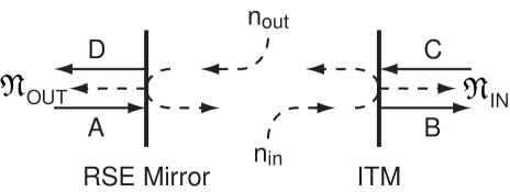
FIG. 16.: Schematic diagram of a simplified version of the RSE cavity. The quantities $\tilde{n}_{\rm in}$ and $\tilde{n}_{\rm out}$ enter inside the RSE cavity, whereas $\mathfrak{N}_{\rm in}$ and $\mathfrak{N}_{\rm out}$ are external to the cavity and exist in different locations.

The fields $\tilde{\mathfrak{N}}_{\rm IN}$ and $\tilde{\mathfrak{N}}_{\rm OUT}$ both have a power spectral density a factor $\sim 1/T_{\mathrm{i}}$ larger than the one-time loss coefficient. This can be explained by the fact that the sideband light bounces back and forth inside the RSE cavity roughly $\sim 1/T_{\mathrm{i}}$ times before exiting. As a result, the (power) loss coefficient is amplified by the same factor. However, since these fields are quite correlated (both contain similar amounts of $\tilde{n}_{\mathrm{in}}$ and $\tilde{n}_{\mathrm{out}}$), we need to analyze them carefully.

For the shot noise, we need to find the amplitude of the vacuum fluctuations that the loss introduces into the output. To understand the effect of this type of loss, we ask how much vacuum fluctuation is added to the field $D$ by $\tilde{\mathfrak{N}}_{\mathrm{IN}}$ and $\tilde{\mathfrak{N}}_{\mathrm{OUT}}$. The answer is obtained by propagating $\tilde{\mathfrak{N}}_{\mathrm{IN}}$ one round trip inside the interferometer’s arm(s) and then combining it with $\tilde{\mathfrak{N}}_{\mathrm{OUT}}$. This gives

$$D \rightarrow D+\left[\tilde{\mathfrak{N}}_{\mathrm{OUT}}+e^{2i\omega L/c}\tilde{\mathfrak{N}}_{\mathrm{IN}}\right]$$ (B69)

$$\approx D+\sqrt{\frac{\varepsilon_{\mathrm{RSE}}T_{\mathrm{i}}}{4}\left(1+\frac{\omega^{2}}{\delta_{\mathrm{i}}^{2}}\right)}$$ (B71)

$$\qquad\times\left(e^{i\beta_{\mathrm{i}}}\tilde{n}_{\mathrm{in}}+e^{-i\beta_{\mathrm{i}}}\tilde{n}_{\mathrm{out}}\right)\,,$$

where $\delta_{\mathrm{i}}\equiv T_{\mathrm{i}}c/4L$ and $\beta_{\mathrm{i}}\equiv\arctan(\omega/\delta_{\mathrm{i}})$. Propagating this to the output, we get the shot noise contribution to be

$${\mathbf{N}}^{\mathrm{shot}}_{\mathrm{RSE}} = \sqrt{\frac{\varepsilon_{\mathrm{RSE}}T_{\mathrm{i}}}{4T_{\mathrm{o}}}\left(1+\frac{\omega^{2}}{\delta_{\mathrm{i}}^{2}}\right)}e^{i\psi}\frac{\omega\delta}{|\mathcal{L}(\omega)|}\Biggl{[}e^{+i\beta_{\mathrm{i}}}\left(\begin{array}[]{c}\tilde{n}_{\mathrm{in}1}\\ \tilde{n}_{\mathrm{in}2}\end{array}\right)$$ (B77)

$$\qquad\qquad+e^{-i\beta_{\mathrm{i}}}\left(\begin{array}[]{c}\tilde{n}_{\mathrm{out}1}\\ \tilde{n}_{\mathrm{out}2}\end{array}\right)\Biggr{]}\,.$$

This noise is not of the magnitude that Eqs. (B 3) would appear to indicate. Instead of having a coefficient of $\sim\sqrt{\varepsilon_{\mathrm{RSE}}/T_{\mathrm{i}}}$, it has a much smaller value when $\omega\lesssim\delta_{\mathrm{i}}$. The reason is that the two vacuum fluctuations traveling in opposite directions are anticorrelated and largely cancel each other, since they are summed in the outgoing field $D$. This cancellation becomes less perfect as $\omega$ grows and becomes much larger than $\delta_{\mathrm{i}}$. This effect is shown in Fig. 11.

For the RSE contribution to the radiation-pressure noise, we are interested in how much the two noise fields $\tilde{\mathfrak{N}}_{\rm IN}$ and $\tilde{\mathfrak{N}}_{\rm OUT}$ contribute to the carrier amplitude fluctuation at the position of the test masses. Therefore, we ask what the sum of $\tilde{\mathfrak{N}}_{\mathrm{IN}}$ and $\tilde{\mathfrak{N}}_{\mathrm{OUT}}$ is when they combine at the end mirrors of the arm cavities. Since $\tilde{\mathfrak{N}}_{\mathrm{OUT}}$ is superposed on $D$, $\tilde{\mathfrak{N}}_{\mathrm{OUT}}$ must be propagated through the sloshing cavity and back to the arm cavity, where it is combined with $\tilde{\mathfrak{N}}_{\mathrm{IN}}$. There is a phase factor of $e^{i\omega L/c}$ due to the propagation from the internal mirror to the end mirror (in addition to the phases acquired on the way to and inside the sloshing cavity; these are explained below), producing

$$B \rightarrow B+e^{i\omega L/c}\left[\tilde{\mathfrak{N}}_{\mathrm{IN}}-\tilde{\mathfrak{N}}_{\mathrm{OUT}}(1-T_{\mathrm{o}})\frac{e^{2i\beta_{\mathrm{s}}}}{1-T_{\mathrm{o}}e^{2i\beta_{\mathrm{s}}}}\right]$$ (B78)

$$\approx B+2T_{\mathrm{o}}\sqrt{\frac{\varepsilon_{\mathrm{RSE}}}{\mathrm{T}_{\mathrm{i}}}}\Biggl{[}\frac{\omega(\delta_{\mathrm{i}}+\delta)+i\Omega^{2}}{\omega\delta}\tilde{n}_{\mathrm{in}}$$ (B80)

$$\qquad\qquad\qquad\qquad+\frac{\omega(\delta_{\mathrm{i}}-\delta)-i\Omega^{2}}{\omega\delta}\tilde{n}_{\mathrm{out}}\Biggr{]}\,.$$

where $\beta_{\rm s}=\arctan(2\omega/\delta_{\rm s})$ is the phase associated with the sloshing cavity. Propagating the new $B$ to the output produces a radiation-pressure contribution

$${\mathbf{N}}^{\mathrm{rad}\,\mathrm{pres}}_{\mathrm{RSE}} = \sqrt{\frac{\varepsilon_{\mathrm{RSE}}T_{\mathrm{o}}}{\mathrm{T}_{\mathrm{i}}}}e^{2i\psi}\left(\begin{array}[]{cc}0&0\\ -\kappa^{*}&0\end{array}\right)$$ (B89)

$$\times\Biggl{[}\frac{\omega(\delta_{\mathrm{i}}+\delta)+i\Omega^{2}}{\omega\delta}\left(\begin{array}[]{c}\tilde{n}_{\mathrm{in}1}\\ \tilde{n}_{\mathrm{in}2}\end{array}\right)$$

$$\qquad+\frac{\omega(\delta_{\mathrm{i}}-\delta)-i\Omega^{2}}{\omega\delta}\left(\begin{array}[]{c}\tilde{n}_{\mathrm{out}1}\\ \tilde{n}_{\mathrm{out}2}\end{array}\right)\Biggr{]}\,.$$

As before, this noise does not have a magnitude $\sim\sqrt{\varepsilon_{\mathrm{RSE}}/T_{\mathrm{i}}}$; it is much smaller. The reason is that when $\tilde{\mathfrak{N}}_{\mathrm{OUT}}$ travels to the sloshing cavity and back to the arms, it gains two phase shifts. First is a constant phase shift of $\pi$, due to the distance it traveled (twice) between the RSE and sloshing mirror. The other is from the sloshing cavity, where for frequencies much larger than the bandwidth $\delta_{\rm s}$ of the sloshing cavity, this phase shift is roughly $\pi$. Adding these two phase shifts, $\tilde{\mathfrak{N}}_{\mathrm{OUT}}$ will appear roughly unchanged when it combines with $\tilde{\mathfrak{N}}_{\mathrm{IN}}$ in the arm cavity. Since these two vacuum fields are anticorrelated, there is again an effective cancellation between the two noises at frequencies above $\delta_{\rm s}$. This cancellation becomes less complete at low frequencies; see Fig. 11.

We assume the fractional loss $\varepsilon_{\rm RSE}\sim 2\times 10^{-5}$, since it arises primarily from losses in the RSE cavity’s optical elements (mirrors and beam splitter). (See Appendix C for a discussion of the noise due to mode mismatching, which we do not consider here.)

4 Detection and Filter Cavities

First, we consider the losses involved in the detection of the signal (without filter cavities). Two important sources of photon loss are mode mismatching associated with the local oscillator used for frequency-independent homodyne detection ($\varepsilon_{\rm lo}$) and the inefficiency of the photodiode ($\varepsilon_{\rm pd}$). In a squeezed-input speed meter, there will also be a circulator (with fractional loss $\varepsilon_{\rm circ}$) through which the squeezed vacuum is fed into the system and through which the output light will have to pass. These losses have no frequency dependence, so they are modeled by an equation of the form of [Eq. (84)] with

$${\cal E}_{\rm OPC}(\omega)=\varepsilon_{\rm OPC}=\varepsilon_{\rm lo}+\varepsilon_{\rm pd}+\varepsilon_{\rm circ}$$ (B90)

[cf. KLMTV Eq. (104)]. The contribution to the noise is then

$${\mathbf{N}}_{\rm OPC}=\sqrt{\varepsilon_{\rm OPC}}\left(\begin{array}[]{c}\tilde{n}_{\mathrm{OPC}1}\\ \tilde{n}_{\mathrm{OPC}2}\end{array}\right)\;,$$ (B91)

where the $\tilde{n}_{\mathrm{OPC}j}$ are linear combinations of the individual (independent) vacuum fields entering at each location (so the spectral densities of these fields are unity and there are no cross-correlations) and propagated to the output port. KLMTV assumed that each of these losses is about 0.001, giving $\varepsilon_{\rm OPC}\sim 0.003$.

We next turn our attention to optical filters on the output (as in the case of frequency-dependent homodyne detection for a squeezed-variational speed meter, discussed in Sec. IV B). Such cavities will have losses that may contribute significantly to the noises of QND interferometers, as has been seen in KLMTV. In their Sec. VI, KLMTV carried out a detailed analyses of such losses; our investigation is essentially the same as theirs.

The loss in the optical filters can come from scattering or absorption in the cavity mirrors, which can be modeled by attributing a finite transmissivity $T_{\rm e}$ to the end mirrors, as we did for the arm cavities. The effect of lossy filters is again analogous to [Eq. (84)]. This time the loss coefficient $\cal E_{\rm F}(\omega)$ does have some frequency dependence:

$${\cal E}_{\rm F}=2\varepsilon_{\rm mm}+\sum_{J=\rm I,II}\bar{\cal E}_{J}=2\varepsilon_{\rm mm}+\frac{1}{2}\sum_{J=\rm I,II}\left({\cal E}_{J+}+{\cal E}_{J-}\right)\,,$$ (B92)

where $\varepsilon_{\rm mm}\sim 0.001$ is the mode-mismatching into each filter cavity and where

$${\cal E}_{J\pm}=\frac{4T_{e}}{T_{J}\left[1+(\pm\omega/\delta_{J}-\xi_{J})^{2}\right]}$$ (B93)

are the loss coefficents of the two different filter cavities ($J={\rm I,II}$) [cf. Eqs. (103) and (106) of KLMTV]. The noise contribution is

$${\bf N}_{\rm F}=\sqrt{\cal E_{\rm F}}\left(\begin{array}[]{c}\tilde{n}_{\rm F1}\\ \tilde{n}_{\rm F2}\\ \end{array}\right)\;.$$ (B94)

The weak frequency-dependence of ${\cal E}_{\rm F}$ will be neglected (as KLMTV did), giving

$$\varepsilon_{\rm F}\simeq{\cal E}_{\rm F}\sim 0.005$$ (B95)

[cf. Eqs. (107) and (104) of KLMTV]. The value of $\varepsilon_{\rm F}$ may vary slightly for the different optimizations we have used, but it remains less than $0.006$.

C Effects due to Mode-Mismatching:
A Simple Analysis

In the practical implementation of GW interferometers, the mismatching of spatial modes between different optical cavities will degrade the sensitivity because signal power will be lost into higher-order modes and, correspondingly, vacuum noises from those modes will be introduced to the signal. In a way, this is similar to other sources of optical loss discussed in the previous appendix. However, the higher-order modes do not simply get dissipated — they too will propagate inside the interferometer (although with a different propagation law). As a consequence, the exchange of energy between fundamental and higher modes due to mode-mismatching is coherent, and the formalism we have been using for the loss does not apply. In this section, we shall extend our formalism to include one higher-order mode and give an extremely simplified model of the mode-mismatching effects.

In a conventional interferometer (LIGO-I), the mode-mismatching comes predominantly from the mismatch of the mirror shapes between the two arms, which makes the wavefronts from the two arms different at the beam splitter. In particular, the cancellation of the carrier light at the dark port is no longer perfect, and additional (bright-port) noises are introduced into the dark-port output. For our speed meter, a third cavity—the sloshing cavity—has to be matched to the two arm cavities, further complicating the problem.

In order to simplify the situation, we approximate all the waves propagating in the corner station (the region near the beam splitter, where the distances are short enough that ) as following the same phase-propagation law as a plane wave. The only possible source of mismatch is assumed to come from the difference of wavefront shapes (to first order in the fractional difference of the radii of curvature) and waist sizes for the light beams emerging from the two arm cavities and the sloshing cavity. Suppose, in the region of the corner station, we have a fiducial fundamental Gaussian mode $\Psi^{(0)}$ (which is being pumped by the carrier) with waist size $w_{0}$ and wavefront curvature $\alpha_{0}\equiv 1/R_{0}$ that is roughly the same as those of the three cavities:

$$\Psi^{(0)}(x,y)\propto\frac{1}{w_{0}}\exp\left(-\frac{\rho^{2}}{w_{0}^{2}}+ik\frac{\alpha_{0}\rho^{2}}{2}\right)\,,\;\rho=\sqrt{x^{2}+y^{2}}\,.$$ (C1)

At leading order in the mismatches, the fundamental modes of the three cavities (in the region of the corner station), which have waist sizes $w_{\rm J}$ and curvatures $\alpha_{\rm J}\equiv 1/R_{\rm J}$ [${\rm J}=$n, e, or slosh (for the north arm, east arm, and sloshing cavity, respectively)], can be written in the form:

$$\Psi_{\rm fnd}^{\rm J}(x,y)$$ (C2)

$$\;\propto\frac{1}{w_{0}}\,\exp\left(ikw_{0}^{2}\,\frac{\alpha_{\rm J}-\alpha_{0}}{4}\right)\exp\left(-\frac{\rho^{2}}{w_{0}^{2}}+ik\frac{\alpha_{0}\rho^{2}}{2}\right)$$ (C3)

$$\quad\times\Biggl{\{}1+\left(\frac{w_{\rm J}-w_{0}}{4w_{0}}+ikw_{0}^{2}\frac{\alpha_{\rm J}-\alpha_{\rm 0}}{16}\right)$$ (C4)

$$\qquad\qquad\times\left[H_{2}\left(\frac{\sqrt{2}x}{w_{0}}\right)+H_{2}\left(\frac{\sqrt{2}y}{w_{0}}\right)\right]\Biggr{\}}\,,$$ (C5)

where $H_{2}(u)$ is the second-order Hermite polynomial of $u$. This $\Psi_{\rm fnd}^{\rm J}(\pi,y)$ can be expressed as $\Psi^{(0)}$ plus a small admixture of a higher-order mode $\Psi^{(1)}$, which consists of equal amounts of ${\rm TEM_{02}}$ and ${\rm TEM_{20}}$ modes [and thus is orthogonal to $\Psi^{(0)}$]. This admixture changes the waist size from $\omega_{0}$ to $\omega_{\rm J}$ and the curvature from $\alpha_{0}$ to $\alpha_{\rm J}$. We can choose our fiducial fundamental mode $\Psi^{(0)}$ in such a way that the two arm cavities have an opposite mismatch with it, i.e., $\alpha_{\rm n}+\alpha_{\rm e}=2\alpha_{0}$, $w_{\rm n}+w_{\rm e}=2w_{0}$, and at leading order,

$$\left(\begin{array}[]{c}\Psi_{\rm fnd}^{\rm n,\,e}\\ \Psi_{\rm exc}^{\rm n,\,e}\end{array}\right)=\left(\begin{array}[]{cc}1&\pm\mu_{\rm arm}\\ \mp\mu_{\rm arm}^{*}&1\end{array}\right)\left(\begin{array}[]{c}\Psi^{(0)}\\ \Psi^{(1)}\end{array}\right)\,,$$ (C6)

where “exc” denotes the excited mode and the admixing amplitude $\mu_{\rm arm}$ is, in general, complex. We also denote the fundamental and excited modes of the sloshing cavity as

$$\left(\begin{array}[]{c}\Psi_{\rm fnd}^{\rm slosh}\\ \Psi_{\rm exc}^{\rm slosh}\end{array}\right)=\left(\begin{array}[]{cc}1&\mu_{\rm slosh}\\ -\mu_{\rm slosh}^{*}&1\end{array}\right)\left(\begin{array}[]{c}\Psi^{(0)}\\ \Psi^{(1)}\end{array}\right)\,;$$ (C7)

again, $\mu_{\rm slosh}$ can be complex. We shall also assume that the higher-order modes involved here are far from resonance inside the cavities and will be rejected by them, gaining a phase of $\pi$ upon reflection from each cavity’s input mirror. In the output, we assume the mode $\Psi^{(0)}$ is selected for detection. (The local oscillator associated with the homodyne detection is chosen to have the same spatial mode as $\Psi^{(0)}$, thereby “selecting” $\Psi^{(0)}$. Note that the potential mode-mismatch effect here is already taken into account in the fractional loss $\varepsilon_{\rm lo}$ of the local oscillator, as described in Sec. B 4.)

Quite naturally, we have to introduce two sets of quadrature operators to describe the two modes. For example, for the field $P(\zeta)$ entering through the extraction mirror, we have

$${\bf\tilde{p}}^{(0)}\equiv\left(\begin{array}[]{c}\tilde{p}_{1}^{(0)}\\ \tilde{p}_{2}^{(0)}\end{array}\right)\,,\quad{\bf\tilde{p}}^{(1)}\equiv\left(\begin{array}[]{c}\tilde{p}_{1}^{(1)}\\ \tilde{p}_{2}^{(1)}\end{array}\right)\,.$$ (C8)

For each of the three cavities, we have to decompose the optical field into its own fundamental and excited modes, propagate them separately and then combine them. The input–output ($a$–$b$) relation of one of the cavities with mirrors held fixed can be written as

$$\left(\begin{array}[]{c}{\bf\tilde{b}^{(0)}}\\ {\bf\tilde{b}^{(1)}}\end{array}\right)=\left[e^{i\Phi_{\rm fnd}}{\bf P}_{\rm fnd}+e^{i\Phi_{\rm exc}}{\bf P}_{\rm exc}\right]\left(\begin{array}[]{c}{\bf\tilde{a}^{(0)}}\\ {\bf\tilde{a}^{(1)}}\end{array}\right)\,,$$ (C9)

where

$${\bf P}_{\rm fnd} = \left(\begin{array}[]{c}1\\ \mu\end{array}\right)\left(\begin{array}[]{cc}1&\mu^{*}\end{array}\right)\,,$$ (C14)

$${\bf P}_{\rm exc} = \left(\begin{array}[]{c}-\mu^{*}\\ 1\end{array}\right)\left(\begin{array}[]{cc}-\mu&1\end{array}\right)\,,$$ (C18)

are the projection operators, and $\Phi_{\rm fnd}$ and $\Phi_{\rm exc}=\pi$ are the phases gained by the fundamental mode and excited mode after being reflected back by the cavity.

The mode-mismatching can cause both shot and radiation pressure noises at the output, giving:

$${\bf\tilde{q}^{(0)}}\rightarrow{\bf\tilde{q}^{(0)}}+{\bf N}^{\rm shot}_{\rm MM}+{\bf N}^{\rm rad\,pres}_{\rm MM}\,.$$ (C19)

Assuming the mirrors are held fixed and applying the new input–output relations (C9) of the non-perfect cavities, we get the following shot noise in the output (to leading order in $\mu_{\rm arm}$ and $\mu_{\rm slosh}$):

$${\bf N}_{\rm MM}^{\rm shot} = -e^{i\psi}{\mu_{\rm arm}^{*}}\sqrt{\frac{4}{T_{\rm o}}}\frac{\sqrt{T_{\rm p}}}{1+\sqrt{1-T_{\rm p}}}$$ (C21)

$$\qquad\qquad\times\frac{1-\sqrt{1-T_{\rm i}}}{\sqrt{T_{\rm i}}}\frac{\omega\delta}{|{\cal L}(\omega)|}\,{\bf\tilde{i}^{(1)}}$$

$$\approx e^{-i\psi}\mu^{*}_{\rm arm}\sqrt{\frac{T_{\rm i}T_{\rm p}}{4T_{\rm o}}}\frac{\omega\delta}{|{\cal L}(\omega)|}{\bf\tilde{i}^{(1)}}\,;$$ (C22)

see Eq. (B1). The quantity ${\bf\tilde{i}^{(1)}}$ refers to the excited mode of the noise coming in the bright port [$I(\zeta)$ in Fig. 3].

The main results embedded in Eq. (C22) are

• the mode-mismatching with the sloshing cavity does not give any contribution at leading order in $\mu$, and

• the mode-mismatching shot noise comes from the higher-order mode entering from the bright port, strongly suppressed by the presence of the internal and power-recycling mirrors.

These two effects are both due to the coherent interaction between the fundamental ($\Psi^{(0)}$) and excited ($\Psi^{(1)}$) modes (of our idealized cavity), in which energy is not simply dissipated from $\Psi^{(0)}$ but exchanged coherently between the two modes as the light flows back and forth between the sloshing cavity and the arm cavities. Detecting an appropriate linear combination of the two modes can then be expected to reverse the effect of mode mismatching. In our case, the properties of the cavities are carefully chosen such that $\Psi^{(0)}$ itself is the desired detection mode (for the sloshing mismatch). Consequently, the mode mismatching with the sloshing cavity does not contribute at leading order [item (i) above]. Regarding item (ii), the mismatch of the two arm cavities does give rise to an additional noise, but it can only come from the higher mode in the bright port, because at leading order in mismatches, (a) the propagation of $\Psi^{(0)}$ from the bright port to the dark port is suppressed and (b) there is no propagation of dark-port $\Psi^{(1)}$ into dark-port $\Psi^{(0)}$ since we have chosen $\Psi^{(0)}$ in such a way that the two arm cavities have exactly opposite mismatches with it.

The reason why this noise is suppressed by the factor $1/T_{\rm p}$ is simple: because $\Psi^{(1)}$ is not on resonance with the composite cavity formed by the power-recycling mirror and the arm cavities, its fluctuations inside the system (like its classical component) are naturally suppressed by a factor $1/\sqrt{T_{\rm p}}$ compared to the level outside the cavity. The reason for the factor of $1/T_{\rm i}$ is similar: the $\Psi^{(1)}$ mode does not resonate within the system formed by the arm cavities and the RSE mirror and will consequently be suppressed.

By computing at the fields at the end mirrors and from them the fluctating radiation pressure, we obtain the radiation-pressure noise due to mode-mismatching:

$${\bf N}_{\rm MM}^{\rm rad\,pres}=-\frac{e^{2i\psi}}{2}\mu_{\rm arm}^{*}\sqrt{\frac{T_{\rm i}T_{\rm p}}{4T_{\rm o}}}\left(\begin{array}[]{cc}0&0\\ -\kappa^{*}&0\end{array}\right){\bf\tilde{i}^{(1)}}\,.$$ (C23)

This radiation-pressure noise is suppressed by a factor similar to the shot noise.

By comparing Eqs. (C22) and (C23) with, e.g., Eqs. (B35), we see that mode mismatching produces noise with essentially the same form as optical-element losses from the arms, extraction mirror and sloshing cavity (AES), with (assuming the input laser is shot-noise limited in the higher modes)

$$\varepsilon_{\rm MM}=\frac{T_{\rm i}T_{\rm p}}{4}|\mu_{\rm arm}^{*}|^{2}\,.$$ (C24)

The factor $T_{\rm i}T_{\rm P}/4$ happens to be the ratio between the input power (at the power-recycling mirror) and the circulating power, which will be $\sim 10^{-4}$. Suppose $\Re(\mu_{\rm arm})\sim\Im(\mu_{\rm arm})\sim 0.03$. The effect of mode-mismatching will then be much less significant (in our simple model) than the losses from the optical elements.

It should be evident that other imperfections in the cavity mirrors, which cause admixtures of other higher-order (“excited”) modes, will lead to similar “dissipation factors,” ${\cal E}_{\rm MM}\sim\frac{T_{\rm i}T_{\rm p}}{4}|\mu^{*}_{\rm arm}|^{2}$. For this reason, we expect mode mismatching to contribute negligibly to the noise, and we ignore it in the body of the paper.

D Transmissivity Mismatch between the Internal Mirror and the RSE Mirror

Recall from Sec. I that when the internal and RSE mirrors have the same transmissivity, their effects on the gravity-wave sideband cancel. If, however, the transmissivity of the internal mirror, $T_{\mathrm{i}}$, is not perfectly matched by that of the RSE mirror, $T_{\mathrm{RSE}}$, then this cancellation will no longer be perfect. As a result, the RSE cavity (i.e., the cavity between the internal and RSE mirrors) will have the same effect as an additional mirror (with a small reflectivity). Suppose the transmissivity of this effective mirror is $T_{\mathrm{RSE}}=(1+\varepsilon_{\mathrm{RSE}})T_{\mathrm{i}}$. Then a simple calculation yields its (amplitude) reflectivity:

$$\mu=\frac{\sqrt{1-T_{\mathrm{i}}}-\sqrt{1-T_{\mathrm{RSE}}}}{1-\sqrt{1-T_{\mathrm{i}}}\sqrt{1-T_{\mathrm{RSE}}}}\approx\frac{\varepsilon_{\mathrm{RSE}}}{2\sqrt{1-T_{\mathrm{i}}}}\approx\frac{\varepsilon_{\mathrm{RSE}}}{2}\,.$$ (D1)

Adding this effective mirror with reflectivity $\mu$ to our interferometer yields a new set of input–output relations similar to Eq. (III A), but with modified $\kappa$ and $\psi$. The functional form of $\kappa$ can be maintained by appropriately redefining the quantities $\Omega$ and $\delta$. To leading order in $\mu$, we obtain

$$\kappa\rightarrow\kappa_{\mathrm{TM}}=\frac{\Omega_{\mathrm{I}}^{3}\delta_{\mathrm{TM}}}{(\omega^{2}-\Omega_{\mathrm{TM}}^{2})^{2}+\omega^{2}\delta^{2}_{\mathrm{TM}}}\,,$$ (D2)

with

$$\Omega\rightarrow\Omega_{\mathrm{TM}}=(1-\mu)\Omega\,,\quad\delta\rightarrow\delta_{\mathrm{TM}}=(1-2\mu)\delta\,.$$ (D3)

Consequently, we can re-optimize the system to compensate for this transmissivity-mismatch effect.

REFERENCES

- [1] C. M. Caves, Phys. Rev. Lett. 45, 75 (1980).
- [2] A. Abramovici et al., Science 256, 325 (1992).
- [3] B. C. Barish and R. Weiss, Physics Today 52, 44 (1999).
- [4] W. G. Unruh, in Quantum Optics, Experimental Gravitation, and Measurement Theory, eds. P. Meystre and M. O. Scully (Plenum, 1982), p. 647.
- [5] M. T. Jaekel and S. Reynaud, Europhys. Lett. 13, 301 (1990).
- [6] E. Gustafson, D. Shoemaker, K. Strain, and R. Weiss, LSC White Paper on Detector Research and Development, LIGO document T990080-00-D (1999); available along with other relevant information at http://www.ligo.caltech.edu/ligo2/ .
- [7] H. J. Kimble, Yu. Levin, A. B. Matsko, K. S. Thorne, and S. P. Vyatchanin, Phys. Rev. D 65, 022002 (2001); cited in text as KLMTV.
- [8] P. Purdue, Phys. Rev. D 66, 022001 (2002); cited in text as Paper I.
- [9] V. B. Braginsky and F. Ya. Khalily, Phys. Lett. A 218, 167 (1996); V. B. Braginsky, M. L. Gorodetsky, and F. Ya. Khalili, Phys. Lett. A 232, 340 (1997).
- [10] V. B. Braginsky, M. L. Gorodetsky, and F. Ya. Khalili, Phys. Lett. A 246, 485 (1998); quant-ph/9806081.
- [11] F. Ya. Khalili, qr-qc/0203002.
- [12] V. B. Braginsky and F. Ya. Khalili, Phys. Lett. A 147, 251 (1990).
- [13] V. B. Braginsky, M. L. Gorodetsky, F. Ya. Khalili, and K. S. Thorne, Phys. Rev. D 61, 044002 (2000); cited in text as BGKT.
- [14] C. M. Caves, Phys. Rev. D 23, 1693 (1981).
- [15] J. Mizuno, Ph.D. thesis, Max Planck Institute für Quantenoptik, 1995.
- [16] A. Freise, G. Heinzel, K. A. Strain, J. Mizuno, K. D. Skeldon, H. Lück, B. Wilke, R. Schilling, A. Rüdiger, W. Wingler and K. Danzmann, Phys. Lett. A 277, 135 (2000)
- [17] J. Mason, Ph.D. thesis, California Institute of Technology, 2001; also available as LIGO document P010010-00-R at www.ligo.caltech.edu/docs/P/P010010-00.pdf .
- [18] C. M. Caves and B. L. Schumaker, Phys. Rev. A 31, 3068 (1985).
- [19] B. L. Schumaker and C. M. Caves, Phys. Rev. A 31, 3093 (1985).
- [20] V. B. Braginsky, M. L. Gorodetsky, F. Ya. Khalili and K. S. Thorne, “Energetic Quantum Limit in Large-Scale Interferometers,” in Gravitational Waves, Proceedings of the Third Edoardo Amaldi Conference, AIP Conference Proceedings Vol. 523, ed. Sydney Meshkov (American Institute of Physics, 2000) pp. 180–192; gr-qc/9907057.
- [21] M. Xiao, L.-A. Wu and H. J. Kimble, Phys. Rev. Lett. 59 278 (1987).
- [22] P. Grangier, R. E. Slusher, B. Yurke and A. La Porta, Phys. Rev. Lett. 59, 2153 (1987).
- [23] K. S. Thorne (private communication).
- [24] S. P. Vyatchanin and A. B. Matsko, JETP 77, 218 (1993).
- [25] S. P. Vyatchanin and E. A. Zubova, Phys. Lett. A 203, 269 (1995).
- [26] S. P. Vyatchanin and A. B. Matsko, JETP 82, 1007 (1996).
- [27] S. P. Vyatchanin and A. B. Matsko, JETP 83, 690 (1996).
- [28] S. P. Vyatchanin, Phys. Lett. A 239, 201 (1998).