Scaling law in signal recycled laser-interferometer gravitational-wave detectors

Abstract

By mapping the signal-recycling (SR) optical configuration to a three-mirror cavity, and then to a single detuned cavity, we express SR optomechanical dynamics, input–output relation and noise spectral density in terms of only three characteristic parameters: the (free) optical resonant frequency and decay time of the entire interferometer, and the laser power circulating in arm cavities. These parameters, and therefore the properties of the interferometer, are invariant under an appropriate scaling of SR-mirror reflectivity, SR detuning, arm-cavity storage time and input power at beamsplitter. Moreover, so far the quantum-mechanical description of laser-interferometer gravitational-wave detectors, including radiation-pressure effects, was only obtained at linear order in the transmissivity of arm-cavity internal mirrors. We relax this assumption and discuss how the noise spectral densities change.

I Introduction

A network of broadband ground-based laser interferometers, aimed at detecting gravitational waves (GWs) in the frequency band $10-10^{4}\,$Hz, is already operating. This network is composed of GEO, the Laser Interferometer Gravitational-wave Observatory (LIGO), TAMA and VIRGO (whose operation will begin in 2004) Inter . The LIGO Scientific Collaboration (LSC) GSSW99 is currently planning an upgrade of LIGO starting from 2008, called advanced LIGO or LIGO-II. Besides the improvement of the seismic isolation and suspension systems, and the increase (decrease) of light power (shot noise) circulating in arm cavities, the LIGO community has planned to introduce an extra mirror, called a signal-recycling mirror (SRM) D82 ; SRt , at the dark-port output (see Fig. 1). The optical system composed of SR cavity and arm cavities forms a composite resonant cavity, whose eigenfrequencies and quality factors can be controlled by the position and reflectivity of the SR mirror. These eigenfrequencies (resonances) can be exploited to reshape the noise curves, enabling the interferometer to work either in broadband or in narrowband configurations, and improving in this way the observation of specific GW astrophysical sources KT .

The initial theoretical analyses D82 ; SRt and experiments SRe of SR interferometers refer to configurations with low laser power, for which the radiation pressure on the arm-cavity mirrors is negligible and the quantum-noise spectra are dominated by shot noise. When the laser power is increased, the shot noise decreases while the effect of radiation-pressure fluctuation increases. LIGO-II has been planned to work at a laser power for which the two effects are comparable in the observational band $40$–$200$ Hz GSSW99 . Thus, to correctly describe the quantum optical noise in LIGO-II, the results have been complemented by a thorough investigation of the influence of radiation-pressure force on mirror motion KLMTV00 ; BC1 ; BC2 ; BC3 . The analyses revealed that SR interferometers behave as an “optical spring”. The dynamics of the whole optomechanical system, composed of arm-cavity mirrors and optical field, resembles that of a free test mass (mirror motion) connected to a massive spring (optical fields). When the test mass and the spring are not connected (e.g., for very low laser power) they have their own eigenmodes: the uniform translation mode for the free mode and the longitudinal-wave mode for the spring. However, for LIGO-II laser power the test mass is connected to the massive spring and the two free modes get shifted in frequency, so the entire coupled system can resonate at two pairs of finite frequencies. Near these resonances the noise curve can beat the free mass standard quantum limit (SQL) for GW detectors BK92 . Indeed, the SQL is not by itself an absolute limit, it depends on the dynamical properties of the test object (or probe) which we monitor. This phenomenon is not unique to SR interferometers; it is a generic feature of detuned cavities All ; FK and was used by Braginsky, Khalili and colleagues in conceiving the “optical bar” GW detectors OB . However, because the optomechanical system is by itself dynamically unstable, and a careful and precise study of the control system should be carried out BC3 .

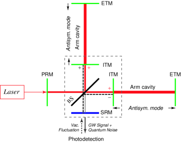
Figure 1: We draw a signal- (and power-) recycled LIGO interferometer. The laser light enters the interferometer from the left (bright port), through the power-recycling mirror (PRM), and get split by a 50/50 beamsplitter (BS) into the two identical (in absence of gravitational waves) arm cavities. Each of the arm cavities is formed by the internal test-mass mirror (ITM) and the end test-mass mirror (ETM). No light leaves the interferometer from below the BS (dark port), except the lights induced by the antisymmetric motion of the test-mass mirrors, e.g., due to a passing-by gravitational wave, or due to vacuum fluctuations that originally enter the interferometer from the dark port. A SRM is placed at the dark port, forming a SR cavity (marked by thick dashed lines) with the ITMs.

The quantum mechanical analysis of SR interferometers given in Refs. BC1 ; BC2 ; BC3 , was built on results obtained by Kimble, Levin, Matsko, Thorne and Vyatchanin (KLMTV) KLMTV00 for conventional interferometers, i.e. without SRM. For this reason, both the SR input–output relation BC1 ; BC2 and the SR optomechanical dynamics BC3 were expressed in terms of parameters characterizing conventional interferometers, such as the storage time in the arm cavities, instead of parameters characterizing SR interferometers as a whole, such as the resonant frequencies and the storage time of the entire interferometer. Therefore, the analysis given in Refs. BC1 ; BC2 ; BC3 is not fully suitable for highlighting the physics in SR interferometers.

In this paper, we first map the SR interferometer into a three-mirror cavity, as originally done by Mizuno JM , though in the low power limit and neglecting radiation-pressure effects, and by Rachmanov MR in classical regimes. Then, as first suggested by Mizuno JM , we regard the very short SR cavity (formed by SRM and ITM) as one (effective) mirror and we express input–output relation and noise spectral density BC1 , and optomechanical dynamics BC2 as well, in terms of three characteristic parameters that have more direct physical meaning: the free optical resonant frequency and decay time of the entire SR interferometer, and the laser power circulating in arm cavities. By free optical resonant frequency and decay time we mean the real and inverse imaginary part of the (complex) optical resonant frequency when all the test-mass mirrors are held fixed. These parameters can then be represented in terms of the more practical parameters: the power transmissivity of ITM, the amplitude reflectivity of SRM, SR detuning and the input power. An appropriate scaling of the practical parameters can leave the characteristic parameters invariant.

In addition, in investigating SR interferometers BC1 ; BC2 ; BC3 the authors restricted the analyses to linear order in the transmissivity of arm-cavity internal mirrors, as also done by KLMTV KLMTV00 for conventional interferometers. In this paper we relax this assumption and discuss how results change.

The outline of this paper is as follows. In Sec. II we explicitly work out the mapping between a SR interferometer and a three-mirror cavity, expressing the free oscillation frequency, decay time and laser power circulating in arm cavity, i.e. the characteristic parameters, in terms of SR-mirror reflectivity, SR detuning and arm-cavity storage time, which are the parameters used in the original description BC1 ; BC2 . An interesting scaling law among the practical parameters is then obtained. In Secs. III and IV.1 the input–output relations, noise spectral density and optomechanical dynamics are expressed in terms of those characteristic parameters. In Sec. IV.2 we map the SR interferometer to a single detuned cavity of the kind analyzed by Khalili FK . In Sec. IV.3 we show that correlations between shot noise and radiation-pressure noise in SR interferometers are equivalent to a change of the optomechanical dynamics, as discussed in a more general context by Syrtsev and Khalili SK94 . In Sec. IV.4, using fluctuation-dissipation theorem, we explain why optical spring detectors have very low intrinsic noise, and are then preferable to mechanical springs in measuring very tiny forces. In Sec. V we derive the input–output relation of SR interferometers at all orders in the transmissivity of internal test-mass mirrors. Finally, Sec. VI summarizes our main conclusions. Appendix A contains definitions and notations, Appendix B discusses the Stokes relations in our optical system and in Appendix C we give the input–output relation including also next-to-leading order terms in the transmissivity of arm-cavity internal mirrors.

In this manuscript we shall be concerned only with quantum noise, though in realistic interferometers seismic and thermal noises are also present. Moreover, we shall neglect optical losses [see Ref. BC2 where optical losses in SR interferometers were discussed].

II Derivation of scaling law

II.1 Equivalent three-mirror–cavity description of signal-recycled interferometer

In Fig. 1, we draw a signal- and power- recycled LIGO interferometer. The Michelson-type optical configuration makes it natural to decompose the optical fields and the mechanical motion of the mirrors into modes that are either symmetric (i.e. equal amplitude) or antisymmetric (i.e. equal in magnitude but opposite in signs) in the two arms, as done in Refs. KLMTV00 ; BC1 ; BC2 ; BC3 , and briefly explained in the following. In order to understand this decomposition more easily, let us for the moment ignore the power-recycling mirror (PRM) and the signal-recycling mirror (SRM).

First, let us suppose all mirrors are held fixed in their equilibrium positions. The laser light, which enters the interferometer from the left of the beamsplitter (BS), excites stationary, monochromatic carrier light inside the two identical arm cavities with equal amplitudes (marked with two + signs in Fig. 1) and thereby drives the symmetric mode. To maximize the carrier amplitude inside the arm cavities, the arm lengths are chosen to be on resonance with the laser frequency. When the carrier lights leave the two arms and recombine at the BS, they have the same magnitude and sign, and, as a consequence, leak out the interferometer only from the left port of the BS. No carrier light leaks out from the port below the BS. For this reason, the left port is called the bright port, and the port below the BS is called the dark port. Obviously, were there any other light that enters the bright port, it would only drive the symmetric mode, which would then leak out only from the bright port. Similarly, lights that enter from the dark port would only drive the antisymmetric optical mode, which have opposite signs at the BS (marked in Fig. 1) and would leak out the interferometer only from the dark port.

Now suppose the mirrors (ITMs and ETMs) move in an antisymmetric (mechanical) mode (shown by arrows in Fig. 1) such that the two arm lengths change in opposite directions — for example driven by a gravitational wave. This kind of motion would pump the (symmetric) carriers in the two arms into sideband lights with opposite signs, which lie in the antisymmetric mode, and would leak out the interferometer from the dark port (and thus can be detected). On the contrary, symmetric mirror motions that change the two arm lengths in the same way would induce sidebands in the symmetric mode, which would leave the interferometer from the bright port. Moreover, sideband lights inside the arm cavities, combined with the strong carrier lights, exert forces on the test masses. Since the carrier lights in the two arms are symmetric, sidebands in the symmetric (antisymmetric) optical mode drive only the symmetric (antisymmetric) mechanical modes. In this way, we have two effectively decoupled systems in our interferometer: (i) ingoing and outgoing bright-port optical fields, symmetric optical and mechanical modes, and (ii) ingoing and outgoing dark-port optical fields, antisymmetric optical and mechanical modes.

When the PRM and SRM are present, since each of them only affects one of the bright/dark ports, the decoupling between the symmetric and antisymmetric modes is still valid. Nevertheless, the behavior of each of the subsystems becomes richer. The PRM, along with the two ITMs, forms a power recycling cavity (for symmetric optical modes, shown by solid lines in Fig. 1). In practice, in order to increase the carrier amplitude inside the arm cavities D82 , this cavity is always set to be on resonance with the input laser light. More specifically, if the input laser power at the PRM is $I_{\rm in}$, then the power input at the BS is $I_{0}=4I_{\rm in}/T_{\rm p}$, and the circulating power inside the arms is $I_{c}=2I_{0}/T$, where $T_{\rm p}$ and $T$ are the power transmissivities of the PRM and the ITM. The SRM, along with the two ITMs, forms a SR cavity (for the antisymmetric optical modes, shown by dashed lines in Fig. 1). By adjusting the length and finesse of this cavity, we can modify the resonant frequency and storage time of the antisymmetric optical mode SRt , and affect the optomechanical dynamics of the entire interferometer BC3 . These changes will reshape the noise curves of SR interferometers, and can allow them to beat the SQL BC1 ; BC2 .

Henceforth, we focus on the subsystem made up of dark-port fields and antisymmetric optical and mechanical modes, in which the detected GW signal and quantum noises reside. In light of the above discussions, it is convenient to identify the two arm cavities as one effective arm cavity, and map the entire interferometer to a three-mirror cavity, as shown in Fig. 2. In particular, the SR cavity, formed by the SRM and ITMs is mapped into a two-mirror cavity (inside the dashed box of Fig. 2) or one effective ITM. The antisymmetric mechanical motions of the two real arm cavities is equal or opposite in sign to those of this system. The input and output fields at the dark port corresponds to those of the three-mirror cavity, $a$ and $b$ (shown in Fig. 2). Because of the presence of the BS in real interferometer (and the absence in effective one), the optical fields inside the two real arms is $\pm 1/\sqrt{2}$ times the fields in the effective cavity composed of the effective ITM and ETM. As a consequence, fields in this effective cavity are $\sqrt{2}$ times as sensitive to mirror motions as those in the real arms, and the effective power in the effective cavity must be

$$I_{\rm arm}=2I_{c}\,.$$ (1)

Therefore, both the carrier amplitude and the sideband amplitude in the effective cavity are $\sqrt{2}$ times stronger than the ones in each real arm. In order to have the same effects on the motion of the mirrors, we must impose the effective ETM and ITM to be twice as massive as the real ones, i.e.

$$m_{\rm arm}=2m\,.$$ (2)

We denote by $T$ and $R=1-T$ the power transmissivity and reflectivity of the ITMs, $L=4$ km is the arm length, and we assume the ETMs to be perfectly reflecting. The arm length is on resonance with the carrier frequency $\omega_{0}=1.8\times 10^{15}\,{\rm sec}^{-1}$, i.e. $\omega_{0}L/c=N\pi$, with $N$ an integer. We denote by $\rho$ and $l$ the reflectivity of the SRM and the length of the SR cavity, and $\phi=[\omega_{0}l/c]_{\mathrm{mod}\,2\pi}$ the phase gained by lights with carrier frequency upon one trip across the SR cavity. We assume the SR cavity to be very short ($\sim 10$ m) compared with the arm-cavity length. Thus, we disregard the phase gained by lights with sideband frequency while traveling across the SR cavity, i.e. $\Omega\,l/c\rightarrow 0$.

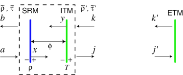
Figure 2: We draw the three-mirror cavity which is equivalent to a SR interferometer in describing the antisymmetric optical/mechanical modes and dark-port optical fields. The SR cavity, which is mapped into a two-mirror cavity (in dashed box) can be viewed as an effective mirror, with four effective reflectivities and transmissivities, $\widetilde{\rho}^{\prime}$, $\widetilde{\tau}^{\prime}$ (for fields entering from the right side), and $\widetilde{\rho}$, $\widetilde{\tau}$ (for fields entering from the left side). The input and output fields, $a$ and $b$, corresponds to those at the dark-port of the real SR interferometer.

The three-mirror cavity system can be broken into two parts. The effective arm cavity, which is the region to the right of the SR cavity, including the ETM (but excluding the ITM), where the light interacts with the mechanical motion of the ETM. This region is completely characterized by the circulating power $I_{c}$, the arm length $L$ and the mirror mass $m$. The (very short) SR cavity, made up of the SRM and the ITM, which does not move. This part is characterized by $T$, $\rho$ and $\phi$.

Henceforth, we assume the radiation pressure forces acting on the ETM and ITM to be equal, and the contribution of the radiation-pressure–induced motion of the two mirrors to the output light, or the radiation-pressure noises due to the two mirrors, to be equal. [These assumptions introduce errors on the order of $\max\{\Omega L/c,\,T\}$.] As a consequence, we can equivalently hold the ITM fixed and assume the ETM has a reduced mass of

$$\mu_{\rm arm}=\frac{1}{2}m_{\rm arm}\,.$$ (3)

II.2 The scaling law in generic form

As first noticed by Mizuno JM , when the SR cavity is very short, we can describe it as a single effective mirror with frequency-independent (but complex) effective transmissivities and reflectivities (see Fig. 2) $\widetilde{\rho}$, $\widetilde{\tau}$ (for fields entering from the left) and $\widetilde{\rho}^{\prime}$, $\widetilde{\tau}^{\prime}$ (for fields entering from the right), and write the following equations for the annihilation (and creation, by taking Hermitian conjugates) operators of the electric field [see Appendix A for notations and definitions]:

$$j_{\pm}(\Omega)=\widetilde{\rho}^{\prime}\,k_{\pm}(\Omega)+\widetilde{\tau}\,a_{\pm}(\Omega)\,,\quad\quad b_{\pm}(\Omega)=\widetilde{\tau}^{\prime}\,k_{\pm}(\Omega)+\widetilde{\rho}\,a_{\pm}(\Omega)\,.$$ (4)

Among these four complex coefficients, $\widetilde{\rho}^{\prime}$, the effective reflectivity from inside the arms, determines the (free) optical resonant frequency $\omega_{0}+\widetilde{\Omega}$ of the system through the relation:

$$\widetilde{\rho}^{\prime}\,e^{2i\widetilde{\Omega}L/c}=1\,.$$ (5)

[Note that the carrier frequency $\omega_{0}$ is assumed to be on resonance in the arm cavity, i.e. $\omega_{0}L/\pi c=\mathrm{integer}$.] It turns out that if we keep fixed the arm-cavity circulating power $I_{c}$, the mirror mass $m$ and the arm-cavity length $L$, the input–output relation $(\widetilde{a}-\widetilde{b})$ of the two-port system (4) is completely determined by $\widetilde{\rho}^{\prime}$ alone or equivalently by the (complex) free optical resonant frequency $\widetilde{\Omega}$. To show this, we first redefine the ingoing and outgoing dark-port fields as:

$$\widetilde{a}_{\pm}(\Omega)=\frac{\widetilde{\tau}}{|\widetilde{\tau}|}\,{a}_{\pm}(\Omega)\,,\quad\quad\widetilde{b}_{\pm}(\Omega)=\frac{\widetilde{\tau}^{*}}{|\widetilde{\tau}|}\,{b}_{\pm}(\Omega)\,.$$ (6)

This redefinition is always possible since we can freely choose another (common) reference point for the input and output fields. Secondly, using the Stokes relations given in the Appendix B, we derive the following equations:

$$j_{\pm}(\Omega) = \widetilde{\rho}^{\prime}\,k_{\pm}(\Omega)+|\widetilde{\tau}|\,\widetilde{a}_{\pm}(\Omega)=\widetilde{\rho}^{\prime}\,k_{\pm}(\Omega)+\sqrt{1-|\widetilde{\rho}^{\prime}|^{2}}\,\widetilde{a}_{\pm}(\Omega)\,,$$ (7)

$$\widetilde{b}_{\pm}(\Omega) = |\widetilde{\tau}|\,k_{\pm}(\Omega)-\widetilde{\rho}^{\prime*}\,\widetilde{a}_{\pm}(\Omega)=\sqrt{1-|\widetilde{\rho}^{\prime}|^{2}}\,k_{\pm}(\Omega)-\widetilde{\rho}^{\prime*}\,\widetilde{a}_{\pm}(\Omega)\,,$$ (8)

from which we infer that the output fields $\widetilde{b}_{\pm}(\Omega)$ depend only on $\widetilde{\rho}^{\prime}$ or equivalently on $\widetilde{\Omega}$. Thus, if we vary the interferometer characteristic parameters $T$, $\rho$ and $\phi$ such that $\widetilde{\rho}^{\prime}$ is preserved, the input–output relation do not change. We refer to the transformation among the interferometer parameters having this property as the scaling law.

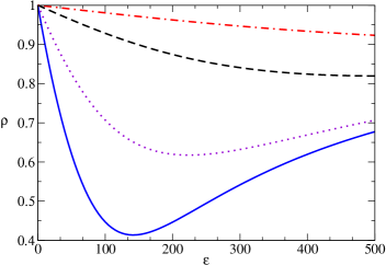
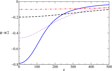
Figure 3: We plot $\rho$ and $\phi-\pi/2$ versus $\epsilon$ for $\lambda=2\pi\times 100\,{\rm Hz}$ (solid line), $2\pi\times 200\,{\rm Hz}$ (dotted line), $2\pi\times 500\,{\rm Hz}$ (dashed line) and $2\pi\times 1000\,{\rm Hz}$ (dashed-dotted line), having fixed $T=0.033$.

II.3 The scaling law in terms of interferometer parameters

In this section we give the explicit expression of the scaling law in terms of the practical parameters of the SR interferometer. We start by deriving the effective transmissivities and reflectivities $\widetilde{\rho}$, $\widetilde{\tau}$, $\widetilde{\rho}^{\prime}$ and $\widetilde{\tau}^{\prime}$ in terms of $T$, $R=1-T$, $\rho$ and $\phi$. By imposing transmission and reflection conditions at the ITM and SRM, and propagating the fields between these mirrors (see Fig. 2), we get the following equations:

$$\tau\,\widetilde{a}_{\pm}(\Omega)+\rho\,e^{i\phi}\,y_{\pm}(\Omega)=x_{\pm}(\Omega)\,,\quad\quad\sqrt{T}\,{k}_{\pm}(\Omega)-\sqrt{R}\,e^{i\phi}\,x_{\pm}(\Omega)=y_{\pm}(\Omega)\,,$$ (9)

$$-\rho\,\widetilde{a}_{\pm}(\Omega)+\tau\,e^{i\phi}\,y_{\pm}(\Omega)=\widetilde{b}_{\pm}(\Omega)\,,\quad\quad\sqrt{R}\,{k}_{\pm}(\Omega)+\sqrt{T}\,e^{i\phi}\,x_{\pm}(\Omega)=j_{\pm}(\Omega)\,,$$ (10)

where the reflection and transmission coefficients of ITM and SRM are chosen to be real, with signs $\{+\sqrt{T},-\sqrt{R}\}$, $\{+\tau,-\rho\}$ for light that impinges on a mirror from outside the SR cavity; and $\{+\sqrt{T},+\sqrt{R}\}$, $\{+\tau,+\rho\}$ for light that impinges on a mirror from inside the SR cavity. Solving Eq. (9) for $x_{\pm}$ and $y_{\pm}$ in terms of $\widetilde{a}_{\pm}$ and $\widetilde{b}_{\pm}$, plugging these expressions into Eq. (10) and comparing with Eq. (4) we obtain:

$$\widetilde{\rho}^{\prime}=\frac{\sqrt{R}+\rho\,e^{2i\phi}}{1+\sqrt{R}\,\rho\,e^{2i\phi}}\,,\quad\quad\widetilde{\rho}=-\frac{\rho+\sqrt{R}\,e^{2i\phi}}{1+\sqrt{R}\,\rho\,e^{2i\phi}}\,,\quad\quad\widetilde{\tau}^{\prime}=\widetilde{\tau}=\frac{\tau\sqrt{T}e^{i\phi}}{1+\sqrt{R}\,\rho\,e^{2i\phi}}\,.$$ (11)

It can be easily verified that these coefficients satisfy the Stokes relations (130)–(131). The scaling law can be obtained by imposing that $\widetilde{\rho}^{\prime}$ does not vary. This gives:

$$\frac{\sqrt{R}+\rho\,e^{2i\phi}}{1+\sqrt{R}\,\rho\,e^{2i\phi}}=\mathrm{const.}\,.$$ (12)

Using Eq. (5), we derive the (complex) free optical resonant frequency in terms of $T$, $\rho$ and $\phi$:

$$\widetilde{\Omega}=\frac{ic}{2L}\log\frac{\sqrt{R}+\rho\,e^{2i\phi}}{1+\sqrt{R}\,\rho\,e^{2i\phi}}\equiv-\lambda-i\,\epsilon\,,$$ (13)

where we trade $\widetilde{\Omega}$ for two real numbers, the resonant frequency $\lambda$ and decay rate (inverse decay time) $\epsilon$. For any choice of $T$, the parameters $\rho$ and $\phi$ can be expressed in terms of $\lambda$ and $\epsilon$ by solving Eq. (13) in terms of $\rho\,e^{2i\phi}$. The result is:

$$\rho\,e^{2i\phi}=\frac{e^{-2\epsilon L/c}e^{2i\lambda L/c}-\sqrt{R}}{1-\sqrt{R}e^{-2\epsilon L/c}e^{2i\lambda L/c}}\,.$$ (14)

In Fig. 3 we plot $\rho$ (left panel) and $\phi-\pi/2$ (right panel) as functions of $\epsilon$ for four typical values of $\lambda$: $2\pi\times 100\,{\rm Hz}$ (solid lines), $2\pi\times 200\,{\rm Hz}$ (dotted lines), $2\pi\times 500\,{\rm Hz}$ (dashed lines) and $2\pi\times 1000\,{\rm Hz}$ (dashed-dotted lines), while fixing $T=0.033$. In Fig. 4, we plot $\rho$ and $\phi-\pi/2$ as functions of $T$, as obtained from Eq. (14), for three sets of optical resonances: $(\lambda,\epsilon)=(2\pi\times 194.5\,{\rm Hz},2\pi\times 25.4\,{\rm Hz})$, plotted in solid lines, which goes through the point $(T,\rho,\phi)=(0.033,0.9,\pi/2-0.47)$ (marked by a square), which is the configuration selected in Refs. BC1 ; BC2 ; BC3 ; $(\lambda,\epsilon)=(2\pi\times 228.1\,{\rm Hz},2\pi\times 69.1\,{\rm Hz})$, plotted in dotted lines, which goes through the point $(T,\rho,\phi)=(0.005,0.96,\pi/2-0.06)$ (marked by a triangle), which is the current LIGO-II reference design LIGOIIref ; and $(\lambda,\epsilon)=(2\pi\times 900\,{\rm Hz},2\pi\times 30\,{\rm Hz})$, plotted in dashed-dotted lines, which is an example of a configuration with narrowband sensitivity around a high frequency. As $T$, $\rho$ and $\phi$ vary along these curves, the input-output relation is preserved.

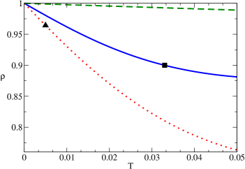
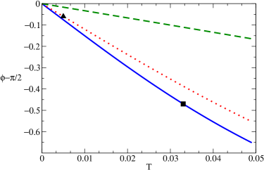
Figure 4: We plot $\rho$ and $\phi-\pi/2$ versus $T$ for three sets of optical resonances: $(\lambda,\epsilon)=(2\pi\times 194.48\,{\rm Hz},2\pi\times 25.42\,{\rm Hz})$ (solid lines), $(\lambda,\epsilon)=(2\pi\times 228.10\,{\rm Hz},2\pi\times 69.13\,{\rm Hz})$ (dotted lines) and $(\lambda,\epsilon)=(2\pi\times 900\,{\rm Hz},2\pi\times 30\,{\rm Hz})$ (dashed-dotted lines). We mark with a square and a triangle the special configurations selected in Refs. BC1 ; BC2 ; BC3 , with $(T,\rho,\phi)=(0.033,0.9,\pi/2-0.47)$, and the current LIGO-II reference design LIGOIIref , with $(T,\rho,\phi)=(0.005,0.96,\pi/2-0.06)$, respectively.

As done in Refs. BC1 ; BC2 , we now expand all the quantities in $T$ and keep only the first nontrivial order. [The accuracy of this procedure will be discussed in Sec. V.] For the crucial quantity $\widetilde{\rho}^{\prime}$ a straightforward calculations gives:

$$\widetilde{\rho}^{\prime}=1-\frac{T}{2}\,\frac{1-\rho\,e^{2i\phi}}{1+\rho\,e^{2i\phi}}\,.$$ (15)

So the scaling law at linear leading order in $T$ is:

$$T\,\frac{1-\rho\,e^{2i\phi}}{1+\rho\,e^{2i\phi}}=\mathrm{const.}\,.$$ (16)

Moreover, applying Eq. (15) to Eq. (5), we derive the following expression for the (free) optical resonant frequency at leading order in $T$:

$$\widetilde{\Omega}=\frac{1}{i}\,\frac{1-\rho\,e^{2i\phi}}{1+\rho\,e^{2i\phi}}\,\frac{Tc}{4L}=\frac{-2\rho\sin 2\phi-i(1-\rho^{2})}{1+\rho^{2}+2\rho\cos 2\phi}\,\gamma\,,$$ (17)

where $\gamma={Tc}/{4L}$ is the half-bandwidth of the arm cavity. The frequency $\widetilde{\Omega}$ coincides with the frequency $\Omega_{-}$ introduced in Ref. BC3 . [Since the authors of Ref. BC3 used the quadrature formalism, they had to introduce another (free) optical resonant frequency which they denoted by $\Omega_{+}=-\Omega_{-}^{*}$. See discussion around Eq. (118) in Appendix A.] Thus, at linear order in $T$ we have:

$$\lambda=\frac{2\rho\,\gamma\,\sin 2\phi}{1+\rho^{2}+2\rho\cos 2\phi}\,,\quad\quad\epsilon=\frac{(1-\rho^{2})\,\gamma}{1+\rho^{2}+2\rho\cos 2\phi}\,.$$ (18)

Finally, using Eqs. (130) and Eq. (15) we obtain the coefficients redefining the fields $a_{\pm}(\Omega)$ and $b_{\pm}(\Omega)$ in Eq. (6):

$$\frac{\widetilde{\tau}}{|\widetilde{\tau}|}=\frac{(1+\rho)\cos\phi+i(1-\rho)\sin\phi}{\sqrt{1+2\rho\cos 2\phi+\rho^{2}}}\,.$$ (19)

III Input–output relation and noise spectral density in terms of characteristic parameters

III.1 Input–output relation

In this section we shall express the input–output relation of SR interferometer (at leading order in $T$) only in terms of the (free) optical resonant frequency, $\widetilde{\Omega}=-\lambda-i\,\epsilon$, and the parameter $\iota_{c}$, defined by

$$\iota_{c}=\frac{8\omega_{0}\,I_{c}}{m\,L\,c}\,,$$ (20)

where the circulating power $I_{c}$ is related to the input power at BS $I_{0}$ by:

$$I_{c}=\frac{2}{T}I_{0}\,.$$ (21)

Using Eq. (19) and the results derived in Appendix A [see Eqs. (114), (116) and (117)] we transform Eqs. (6), which are given in terms of annihilation and creation operators, into equations for quadrature fields:

$$\left(\begin{array}[]{c}\widetilde{a}_{1}\\ \widetilde{a}_{2}\end{array}\right)=\frac{1}{\sqrt{1+2\rho\cos 2\phi+\rho^{2}}}\left(\begin{array}[]{cc}(1+\rho)\cos\phi&-(1-\rho)\sin\phi\\ (1-\rho)\sin\phi&(1+\rho)\cos\phi\end{array}\right)\left(\begin{array}[]{c}a_{1}\\ a_{2}\end{array}\right)\,,$$ (22)

and

$$\left(\begin{array}[]{c}\widetilde{b}_{1}\\ \widetilde{b}_{2}\end{array}\right)=\frac{1}{\sqrt{1+2\rho\cos 2\phi+\rho^{2}}}\left(\begin{array}[]{cc}(1+\rho)\cos\phi&(1-\rho)\sin\phi\\ -(1-\rho)\sin\phi&(1+\rho)\cos\phi\end{array}\right)\left(\begin{array}[]{c}b_{1}\\ b_{2}\end{array}\right)\,.$$ (23)

Inserting the above expressions into Eqs. (2.20)–(2.24) of Ref. BC1 , and using Eqs. (18)–(21), we get the input–output relation depending only on the characteristic or scaling invariant quantities $\lambda$, $\epsilon$ and $\iota_{c}$:

$$\left(\begin{array}[]{c}\widetilde{b}_{1}\\ \widetilde{b}_{2}\end{array}\right)=\frac{1}{\widetilde{M}^{(1)}}\,\left\{\left(\begin{array}[]{cc}\widetilde{C}^{(1)}_{11}&\widetilde{C}^{(1)}_{12}\\ \widetilde{C}^{(1)}_{21}&\widetilde{C}^{(1)}_{22}\end{array}\right)\left(\begin{array}[]{c}\widetilde{a}_{1}\\ \widetilde{a}_{2}\end{array}\right)+\left(\begin{array}[]{c}\widetilde{D}^{(1)}_{1}\\ \widetilde{D}^{(1)}_{2}\end{array}\right)\frac{h}{h_{\rm SQL}}\right\}\,,$$ (24)

where we define:

$$\widetilde{M}^{(1)}={\left[\lambda^{2}-(\Omega+i\epsilon)^{2}\right]\,\Omega^{2}-\lambda\,\iota_{c}}\,,$$ (25)

and

$$\widetilde{C}^{(1)}_{11}=\widetilde{C}^{(1)}_{22}=\Omega^{2}(\Omega^{2}-\lambda^{2}+\epsilon^{2})+\lambda\,\iota_{c}\,,\quad\quad\widetilde{C}^{(1)}_{12}=-2\epsilon\,\lambda\,\Omega^{2}\,,\quad\quad\widetilde{C}^{(1)}_{21}=2\epsilon\,\lambda\,\Omega^{2}-2\epsilon\,\iota_{c}\,,$$ (26)

$$\widetilde{D}^{(1)}_{1}=-2\lambda\,\sqrt{\epsilon\,\iota_{c}}\,\Omega\,,\quad\quad\widetilde{D}^{(1)}_{2}=2(\epsilon-i\Omega)\,\Omega\,\sqrt{\epsilon\,\iota_{c}}\,,$$ (27)

and

$$h_{\rm SQL}\equiv\sqrt{\frac{8\hbar}{m\Omega^{2}L^{2}}}\,,$$ (28)

is the free-mass SQL for the gravitational strain $h(\Omega)$ in LIGO detectors BK92 . The quantity $\iota_{c}$ has the dimension of a frequency to the third power ($\Omega^{3}$). Since it is proportional to the laser power circulating in the arm cavity, it provides a measure of radiation-pressure strength. In order that radiation pressure influence interferometer dynamics in the frequency range interesting for LIGO, we need

$$\iota_{c}\,\stackrel{{\scriptstyle>}}{{{}_{\sim}}}\,\Omega_{\rm GW}^{3}\quad\quad\Rightarrow\quad\quad I_{c}\stackrel{{\scriptstyle>}}{{{}_{\sim}}}\frac{m\,L\,c\,\Omega^{3}_{\rm GW}}{8\omega_{0}}\,,$$ (29)

which gives $I_{c}\stackrel{{\scriptstyle>}}{{{}_{\sim}}}100\,$ kW for typical LIGO-II–parameters and $\Omega_{\rm GW}=2\pi\times 100\,$Hz. The input–output relation (24) is more explicit in representing interferometer properties than that given in Ref. BC1 , and can be quite useful in the process of optimizing the SR optical configuration BCM . From the last term of Eq. (24) we observe that as long as the SR oscillation frequency $\lambda\neq 0$, both quadrature fields contain the GW signal. Moreover, the resonant structure, discussed in Ref. BC1 ; BC2 , is readily displayed in the denominator of Eq. (24), given by Eq. (25). As we shall see in Sec. IV, the shot noise and radiation-pressure noise, and the fact they are correlated, can also be easily worked out from Eq. (24).

In Ref. BC3 we found that one of the SR resonant frequencies, obtained by imposing $\widetilde{M}^{(1)}=0$, has always a positive imaginary part, corresponding to an instability. This instability has an origin similar to the dynamical instability induced in a detuned Fabry-Perot cavity by the radiation-pressure force acting on the mirrors All ; OB . To suppress it, we proposed BC3 a feed-back control system that does not compromise the GW interferometer sensitivity. Although the model we used to describe the servo system may be realistic for an all-optical control loop, this might not be the case if an electronic servo system is implemented. However, results obtained in Refs. french would suggest it does. In any case, a more thorough studying should be pursued to fully clarify this issue. In this paper, we always assume that an appropriate control system of the kind proposed in Ref. BC3 is used.

Finally, when $\lambda=0$ (which corresponds to either $\rho=0$, or $\rho\neq 0$, $\phi=0,\,\pi/2$) Eq. (24) simplifies to

$$\left(\begin{array}[]{c}\widetilde{b}_{1}\\ \widetilde{b}_{2}\end{array}\right)=e^{2i\beta^{\prime}}\left(\begin{array}[]{cc}1&0\\ -{\cal K}^{\prime}&1\end{array}\right)\left(\begin{array}[]{c}\widetilde{a}_{1}\\ \widetilde{a}_{2}\end{array}\right)+e^{i\beta^{\prime}}\sqrt{2{\cal K}^{\prime}}\left(\begin{array}[]{c}0\\ 1\end{array}\right)\frac{h}{h_{\rm SQL}}\,,$$ (30)

which exactly coincides with Eq. (16) of Ref. KLMTV00 for a conventional interferometer, but where

$$\beta^{\prime}=\arctan\left(\frac{\Omega}{\epsilon}\right)\,,\quad\quad{\cal K^{\prime}}=\frac{2\,\epsilon\,\iota_{c}}{\Omega^{2}\,(\Omega^{2}+\epsilon^{2})}\,.$$ (31)

The simple relations (30), (31) nicely unify the SR optical configuration $\phi=0,\pi/2$ (denoted by ESR/ERSE in Ref. BC2 ) with the conventional-interferometer optical configuration.

III.2 Noise spectral density

The noise spectral density can be calculated as follows KLMTV00 ; BC1 . Assuming that the quadrature $\widetilde{b}_{\zeta}=\widetilde{b}_{1}\,\sin\zeta+\widetilde{b}_{2}\,\cos\zeta$ is measured, and using Eq. (24), we can express the interferometer noise as an equivalent GW Fourier component:

$$h_{n}\equiv h_{\rm SQL}\,\Delta\widetilde{b}_{\zeta}\,,$$ (32)

where

$$\Delta\widetilde{b}_{\zeta}=\frac{(\widetilde{C}^{(1)}_{11}\,\sin\zeta+\widetilde{C}^{(1)}_{21}\,\cos\zeta)\,\widetilde{a}_{1}+(\widetilde{C}^{(1)}_{12}\,\sin\zeta+\widetilde{C}^{(1)}_{22}\,\cos\zeta)\,\widetilde{a}_{2}}{\widetilde{D}^{(1)}_{1}\,\sin\zeta+\widetilde{D}^{(1)}_{2}\,\cos\zeta}\,.$$ (33)

Then the (single-sided) spectral density $S^{\zeta}_{h}(f)$, with $f=\Omega/2\pi$, associated with the noise $h_{n}$ can be computed by the formula [see Eq. (22) of Ref. KLMTV00 ]:

$$2\pi\,\delta(\Omega-\Omega^{\prime})\,S^{\zeta}_{h}(f)=\langle{\rm in}|h_{n}(\Omega)\,h_{n}^{\dagger}(\Omega^{\prime})+h_{n}^{\dagger}(\Omega^{\prime})\,h_{n}(\Omega)|{\rm in}\rangle\,.$$ (34)

Assuming that the input of the whole SR interferometer is in its vacuum state, i.e. $|{\rm in}\rangle=|0_{\tilde{a}}\rangle$, and using

$$\langle 0_{\tilde{a}}|\widetilde{a}_{i}(\Omega)\,\widetilde{a}^{\dagger}_{j}(\Omega^{\prime})+\widetilde{a}^{\dagger}_{j}(\Omega^{\prime})\,\widetilde{a}_{i}(\Omega)|0_{\tilde{a}}\rangle=2\pi\,\delta(\Omega-\Omega^{\prime})\,\delta_{ij}\,,$$ (35)

we find that Eq. (34) can be recast in the simple form (note that $\widetilde{C}^{(1)}_{ij}\in\Re$):

$$S_{h}^{\zeta}={h_{\rm SQL}^{2}}\,\frac{\left(\widetilde{C}^{(1)}_{11}\,\sin\zeta+\widetilde{C}^{(1)}_{21}\,\cos\zeta\right)^{2}+\left(\widetilde{C}^{(1)}_{12}\,\sin\zeta+\widetilde{C}^{(1)}_{22}\,\cos\zeta\right)^{2}}{\left|\widetilde{D}^{(1)}_{1}\,\sin\zeta+\widetilde{D}^{(1)}_{2}\,\cos\zeta\right|^{2}}\,.$$ (36)

Plugging into the above expression Eqs. (26), (27) we get the very explicit (and very simple!) expression for the noise spectral density:

$$S_{h}^{\zeta} = \frac{\Omega^{2}h_{\rm SQL}^{2}}{4\epsilon\iota_{c}\left[\Omega^{2}\cos^{2}\zeta+(\epsilon\cos\zeta-\lambda\sin\zeta)^{2}\right]}\Bigg{\{}\left[(\Omega+\lambda)^{2}+\epsilon^{2}\right]\left[(\Omega-\lambda)^{2}+\epsilon^{2}\right]+\frac{2\iota_{c}}{\Omega^{2}}\big{[}\Omega^{2}(\lambda-\epsilon\sin 2\zeta)$$ (37)

$$- \lambda(\epsilon^{2}+\lambda^{2}+2\epsilon^{2}\cos 2\zeta)-\epsilon(\epsilon^{2}-\lambda^{2})\sin 2\zeta\big{]}+\frac{\iota_{c}^{2}}{\Omega^{4}}\left[2\epsilon^{2}(1+\cos 2\zeta)-2\epsilon\lambda\sin 2\zeta+\lambda^{2}\right]\Bigg{\}}\,.$$

IV Optomechanical dynamics in terms of characteristic parameters

The scaling laws (14), (16) could have been equivalently derived by imposing the invariance of the optomechanical dynamics BC3 . In this section we express all the relevant quantities characterizing the SR optomechanical dynamics in terms of the scaling invariant parameters $\lambda$, $\epsilon$ and $\iota_{c}$.

IV.1 Radiation-pressure force

In Ref. BC2 we assumed that SR interferometers can be artificially divided into two linearly coupled, but otherwise independent subsystems: the probe ${\cal P}$, which is subject to the external classical GW force $G$ and the detector ${\cal D}$, which yields a classical output $Z$. The Hamiltonian of the overall system is given by [see Sec. IIB in Ref. BC2 for notations and definitions]:

$$H=H_{\cal P}+{H}_{\cal D}-{x}\,({F}+G)\,,$$ (38)

where $x$ is the operator describing the antisymmetric mode of motion of four arm-cavity mirrors and $F$ is the radiation-pressure or back-action force the detector applies on the probe. In the Heisenberg picture, using the superscript ${(1)}$ for operators evolving under the total Hamiltonian ${H}$, and superscript ${(0)}$ for operators evolving under the free Hamiltonian of the detector ${H}_{\cal D}$, the equations of motion in Fourier domain read BC2 :

$${Z}^{(1)}(\Omega) = {Z}^{(0)}(\Omega)+R_{ZF}(\Omega)\,{x}^{(1)}(\Omega)\,,$$ (39)

$${F}^{(1)}(\Omega) = {F}^{(0)}(\Omega)+R_{FF}(\Omega)\,{x}^{(1)}(\Omega)\,,$$ (40)

$${x}^{(1)}(\Omega) = L\,h(\Omega)+R_{xx}(\Omega)\,{F}^{(1)}(\Omega)\,.$$ (41)

where $R_{xx}(\Omega)=-4/m/\Omega^{2}$, $h(\Omega)$ is the gravitational strain [see Eq. (2.15) of Ref. BC3 ] related to the GW force in Fourier domain by $G(\Omega)=-(m/4)\,L\,\Omega^{2}\,h(\Omega)$, while the various Fourier-domain susceptibilities are defined by:

$$R_{AB}(\Omega)\equiv\frac{i}{\hbar}\int_{0}^{+\infty}d\tau\,e^{i\Omega\tau}\,[A(0),B(-\tau)]\,,$$ (42)

where $[A(t),B(t^{\prime})]$ is the commutator between operators $A$ and $B$. As discussed in Sec. I, LIGO-II has been planned to work at a laser power for which shot noise and radiation-pressure noise are comparable in the observational band $40$–$200$ Hz. In Sec. IIIA of Ref. BC2 the radiation-pressure force was explicitly derived. Here, we want to express it, and the other crucial quantities entering the equations of motion (39)–(41) in terms of the characteristic parameters $\lambda$, $\epsilon$ and

$${\cal I}_{c}=m\,\iota_{c}=\frac{8\omega_{0}\,I_{c}}{L\,c}\,.$$ (43)

Using Eqs. (18) a straightforward calculation gives the rather simple expressions:

$$F^{(0)}(\Omega)=\sqrt{\frac{\epsilon{\cal I}_{c}\,\hbar}{2}}\,\frac{(i\Omega-\epsilon)\,\widetilde{a}_{1}(\Omega)+\lambda\,\widetilde{a}_{2}(\Omega)}{(\Omega-\lambda+i\epsilon)\,(\Omega+\lambda+i\epsilon)}\,,$$ (44)

$$Z_{1}^{(0)}(\Omega) = \frac{(\lambda^{2}-\epsilon^{2}-\Omega^{2})\,\widetilde{a}_{1}(\Omega)+2\lambda\,\epsilon\,\widetilde{a}_{2}(\Omega)}{(\Omega-\lambda+i\epsilon)\,(\Omega+\lambda+i\epsilon)}\,,$$ (45)

$$Z_{2}^{(0)}(\Omega) = \frac{-2\lambda\,\epsilon\,\widetilde{a}_{1}(\Omega)+(\lambda^{2}-\epsilon^{2}-\Omega^{2})\,\widetilde{a}_{2}(\Omega)}{(\Omega-\lambda+i\epsilon)\,(\Omega+\lambda+i\epsilon)}\,,$$ (46)

$$R_{Z_{1}F}(\Omega) = \sqrt{\frac{\epsilon{\cal I}_{c}}{2\hbar}}\,\frac{\lambda}{(\Omega-\lambda+i\epsilon)\,(\Omega+\lambda+i\epsilon)}\,,$$ (47)

$$R_{Z_{2}F}(\Omega) = -\sqrt{\frac{\epsilon{\cal I}_{c}}{2\hbar}}\,\frac{(\epsilon-i\Omega)}{(\Omega-\lambda+i\epsilon)\,(\Omega+\lambda+i\epsilon)}\,.$$ (48)

The optical pumping field in detuned Fabry-Perot resonator converts the free test mass into an optical spring having very low intrinsic noise OB . The ponderomotive rigidity $K_{\rm pond.\,rig.}$, which characterizes the optomechanical dynamics in SR interferometers, is also responsible of the beating of the free mass SQL [see Sec. IIIC of Ref. BC3 ] and its explicit expression is given by:

$$K_{\rm pond}(\Omega)=-R_{FF}(\Omega)=-\frac{{\cal I}_{c}}{4}\,\frac{\lambda}{(\Omega-\lambda+i\epsilon)\,(\Omega+\lambda+i\epsilon)}\,.$$ (49)

As long as the free optical resonant frequency $\lambda$ differs from zero, $K_{\rm pond}$ is always non-vanishing. Moreover, in order to have a (nearly) real mechanical resonant frequency at low frequency, we require $\lambda<0$ [as can be obtained by imposing $K_{\rm pond}(\Omega=0)>0$.]

IV.2 Equivalence between noise correlations and change of dynamics

As derived in Ref. BC2 ; BC3 , the output of SR interferometers, when the first or second quadrature of the outgoing dark-port field is measured, can also be written as:

$${\cal O}_{i}(\Omega)={\cal Z}_{i}(\Omega)+R_{xx}(\Omega)\,\left[{\cal F}_{i}(\Omega)+G(\Omega)\right]\,,\quad\quad i=1,2$$ (50)

where:

$${\cal Z}_{i}(\Omega)=\frac{Z^{(0)}_{i}(\Omega)}{R_{Z_{i}F}(\Omega)}\,,\quad{\cal F}(\Omega)=F^{(0)}(\Omega)-R_{FF}(\Omega)\frac{Z_{i}^{(0)}(\Omega)}{R_{Z_{i}F}(\Omega)}\,,\quad\quad i=1,2\,.$$ (51)

Expressing these quantities in scaling-invariant form [here the first or second quadrature refers to $\widetilde{b}_{1}$ or $\widetilde{b}_{2}$, so the $Z_{1,2}$ discussed here are related to those in Ref. BC2 by the rotation (23)], we get:

$${\cal Z}_{1}(\Omega) = \sqrt{\frac{2\hbar}{\epsilon{\cal I}_{c}}}\,\frac{1}{\lambda}\,\left[(\lambda^{2}-\epsilon^{2}-\Omega^{2})\,\widetilde{a}_{1}(\Omega)+2\epsilon\,\lambda\,\widetilde{a}_{2}(\Omega)\right]\,,$$ (52)

$${\cal Z}_{2}(\Omega) = \sqrt{\frac{2\hbar}{\epsilon{\cal I}_{c}}}\,\frac{1}{(\epsilon-i\Omega)}\,\left[2\epsilon\,\lambda\,\widetilde{a}_{1}(\Omega)-(\lambda^{2}-\epsilon^{2}-\Omega^{2})\,\widetilde{a}_{2}(\Omega)\right]\,,$$ (53)

and

$${\cal F}_{1}(\Omega) = \sqrt{\frac{{\cal I}_{c}\,\hbar}{8\,\epsilon}}\,\widetilde{a}_{1}(\Omega)\,,$$ (54)

$${\cal F}_{2}(\Omega) = \sqrt{\frac{{\cal I}_{c}\,\hbar}{8\,\epsilon}}\,\frac{1}{(\epsilon-i\Omega)}\,\left[2\epsilon\,\widetilde{a}_{1}(\Omega)-\lambda\,\widetilde{a}_{2}(\Omega))\right]\,.$$ (55)

The form of Eq. (50), along with the fact that the operators ${\cal Z}_{i}(\Omega)$ and ${\cal F}_{i}(\Omega)$ are proportional to $1/\sqrt{I_{c}}$ and $\sqrt{I_{c}}$, made it natural to refer to them BC3 as effective output fluctuation and effective radiation-pressure force. The quantum noise embodied in ${\cal Z}_{i}(\Omega)$ is the shot noise, while the quantum noise described by ${\cal F}_{i}(\Omega)$ is the radiation-pressure or back-action noise. The operators ${\cal Z}_{i}(\Omega)$, ${\cal F}_{i}(\Omega)$ satisfy the following commutation relations BK92 ; BC2 ; BC3 :

$$[{\cal Z}_{i}(\Omega),{\cal Z}_{i}^{\dagger}(\Omega^{\prime})]=0=[{\cal F}_{i}(\Omega),{\cal F}_{i}^{\dagger}(\Omega^{\prime})]\,,\quad\quad[{\cal Z}_{i}(\Omega),{\cal F}_{i}^{\dagger}(\Omega^{\prime})]=-2\pi\,i\,\hbar\,\delta(\Omega-\Omega^{\prime})\,,\quad\quad i=1,2\,.$$ (56)

If the output quadrature $i$ is measured, the noise spectral density (36), written in terms of the operators ${\cal Z}_{i}$ and ${\cal F}_{i}$, reads BK92 :

$$S_{h,i}(\Omega)=\frac{1}{L^{2}}\,\left\{S_{{\cal Z}_{i}{\cal Z}_{i}}(\Omega)+2{\cal R}_{xx}(\Omega)\,\Re\left[S_{{\cal F}_{i}{\cal Z}_{i}}(\Omega)\right]+{\cal R}_{xx}^{2}(\Omega)\,S_{{\cal F}_{i}{\cal F}_{i}}(\Omega)\right\}\,,$$ (57)

where the (one-sided) cross spectral density of two operators is expressible, by analogy with Eq. (34), as

$$2\pi\,\delta\left(\Omega-\Omega^{\prime}\right)\,S_{{\cal A}{\cal B}}(\Omega)=\langle 0_{\tilde{a}}|{\cal A}(\Omega){\cal B}^{\dagger}(\Omega^{\prime})+{\cal B}^{\dagger}(\Omega^{\prime}){\cal A}(\Omega)|0_{\tilde{a}}\rangle\,.$$ (58)

In Eq. (57), the terms containing $S_{{\cal Z}_{i}{\cal Z}_{i}}$, $S_{{\cal F}_{i}{\cal F}_{i}}$ and $\Re\left[S_{{\cal F}_{i}{\cal Z}_{i}}\right]$ should be identified as shot noise, radiation-pressure noise and a term proportional to the correlation between the two noises, respectively BK92 . The noise spectral densities expressed in terms of the scaling invariant quantities $\lambda$, $\epsilon$ and ${\cal I}_{c}$ are rather simple and read:

$$S_{{\cal Z}_{1}{\cal Z}_{1}}(\Omega) = \frac{2\hbar}{{\cal I}_{c}}\,\frac{\left[(\Omega+\lambda)^{2}+\epsilon^{2}\right]\left[(\Omega-\lambda)^{2}+\epsilon^{2}\right]}{\epsilon\,\lambda^{2}}\,,$$ (59)

$$S_{{\cal Z}_{2}{\cal Z}_{2}}(\Omega) = \frac{2\hbar}{{\cal I}_{c}}\,\frac{\left[(\Omega+\lambda)^{2}+\epsilon^{2}\right]\left[(\Omega-\lambda)^{2}+\epsilon^{2}\right]}{\epsilon\,(\epsilon^{2}+\Omega^{2})}\,,$$ (60)

$$S_{{\cal F}_{1}{\cal F}_{1}}(\Omega) = \frac{\hbar{\cal I}_{c}}{8\,\epsilon}\,,$$ (61)

$$S_{{\cal F}_{2}{\cal F}_{2}}(\Omega) = \frac{\hbar{\cal I}_{c}}{8\,\epsilon}\,\frac{(4\epsilon^{2}+\lambda^{2})}{\epsilon^{2}+\Omega^{2}}\,,$$ (62)

$$S_{{\cal Z}_{1}{\cal F}_{1}}(\Omega) = \hbar\,\frac{(\lambda^{2}-\epsilon^{2}-\Omega^{2})}{2\epsilon\,\lambda}\,,$$ (63)

$$S_{{\cal Z}_{2}{\cal F}_{2}}(\Omega) = \hbar\,\frac{\lambda\,(\lambda^{2}+3\epsilon^{2}-\Omega^{2})}{2\epsilon\,(\epsilon^{2}+\Omega^{2})}\,.$$ (64)

Note that in our case $S_{{\cal F}_{i}{\cal Z}_{i}}$ is real, thus $S_{{\cal F}_{i}{\cal Z}_{i}}=S_{{\cal Z}_{i}{\cal F}_{i}}$. It is straightforward to check that the following relation is also satisfied:

$$S_{{\cal Z}_{i}{\cal Z}_{i}}(\Omega)\,S_{{\cal F}_{i}{\cal F}_{i}}(\Omega)-S_{{\cal Z}_{i}{\cal F}_{i}}(\Omega)\,S_{{\cal F}_{i}{\cal Z}_{i}}(\Omega)=\hbar^{2}\,,\quad\quad i=1,2\,.$$ (65)

Since in SR interferometers $S_{{\cal Z}_{i}{\cal F}_{i}}\neq 0$, the noise spectral density $S_{h,i}$ is not limited by the free-mass SQL for GW interferometers ($S_{\rm SQL}\equiv h^{2}_{\rm SQL}$), as derived and discussed in Refs. BC1 ; BC2 ; BC3 .

We want to show now that cross correlations between shot noise and radiation-pressure noise are equivalent to some modification of the optomechanical dynamics of the system composed of probe and detector, as originally pointed out by Syrtsev and Khalili in Sec. III of Ref. SK94 . More specifically, we shall show that for linear quantum measurement devices, at the cost of modifying the optomechanical dynamics, the measurement process can be described in terms of new operators ${\cal Z}^{\prime}$ and ${\cal F}^{\prime}$ with zero cross correlation.

In Ref. BC2 the authors found that the most generic transformation which preserves the commutation relations (56) is of the form [see Eq. (2.25) in Ref. BC2 ]:

$$\left(\begin{array}[]{c}{\cal Z}_{i}^{\prime}(\Omega)\\ {\cal F}_{i}^{\prime}(\Omega)\end{array}\right)=e^{i\alpha}\,\left(\begin{array}[]{cc}L_{11}&L_{12}\\ L_{21}&L_{22}\end{array}\right)\left(\begin{array}[]{c}{\cal Z}_{i}(\Omega)\\ {\cal F}_{i}(\Omega)\end{array}\right)\,,$$ (66)

with $\alpha,\,L_{ij}\in\Re$ and $\det L_{ij}=1$. Under this transformation the output (50) becomes:

$${\cal O}_{i}(\Omega)=e^{-i\alpha}\,\left[L_{22}-R_{xx}(\Omega)\,L_{21}\right]\,{\cal Z}^{\prime}_{i}(\Omega)+e^{-i\alpha}\,\left[-L_{12}+R_{xx}(\Omega)\,L_{11}\right]\,{\cal F}^{\prime}_{i}(\Omega)+R_{xx}(\Omega)\,G(\Omega)\,.$$ (67)

By imposing that the system responds in the same way to electromagnetic and gravitational forces, ${\cal F}^{\prime}(\Omega)$ and $G(\Omega)$, we find the two conditions: $e^{i\alpha}=\pm 1$ and $R_{xx}(\Omega)\,(L_{11}\mp 1)=L_{12}$. The transformation we have to apply so that the correlations between new fields ${\cal Z}^{\prime}_{i}(\Omega)$ and ${\cal F}_{i}^{\prime}(\Omega)$ are zero, give the following set of equations:

$$L\,\left(\begin{array}[]{cc}S_{{\cal Z}_{i}{\cal Z}_{i}}(\Omega)&S_{{\cal Z}_{i}{\cal F}_{i}}(\Omega)\\ S_{{\cal F}_{i}{\cal Z}_{i}}(\Omega)&S_{{\cal F}_{i}{\cal F}_{i}}(\Omega)\end{array}\right)\,L^{t}=\left(\begin{array}[]{cc}S_{{\cal Z}_{i}^{\prime}{\cal Z}^{\prime}_{i}}(\Omega)&0\\ 0&S_{{\cal F}_{i}^{\prime}{\cal F}_{i}^{\prime}}(\Omega)\end{array}\right)\,.$$ (68)

When $S_{\cal ZF}=S_{\cal FZ}\in\Re$, as it happens in SR interferometers, the above conditions can be solved in infinite ways. A simple solution, suggested by Syrtsev and Khalili SK94 , is obtained by taking $\alpha=0$ and $L_{11}=1$. In this case, a straightforward calculation gives: $L_{12}=0$, $L_{21}=-S_{{\cal Z}_{i}{\cal F}_{i}}/S_{{\cal Z}_{i}{\cal Z}_{i}}$ and $L_{22}=1$. The output becomes:

$${\cal O}^{\prime}_{i}(\Omega)={\cal Z}^{\prime}_{i}(\Omega)+\chi_{i}^{\rm eff}(\Omega)\,\left[{\cal F}^{\prime}_{i}(\Omega)+G(\Omega)\right]\,,\quad\quad{\cal O}^{\prime}_{i}(\Omega)={\cal O}_{i}(\Omega)\,\frac{R_{xx}(\Omega)}{\chi_{i}^{\rm eff}(\Omega)}\,,$$ (69)

where $\chi_{i}^{\rm eff}$, the effective susceptibility, is given by:

$$\chi_{i}^{\rm eff}(\Omega)=\frac{R_{xx}(\Omega)}{1+R_{xx}(\Omega)\,S_{{\cal Z}_{i}{\cal F}_{i}}(\Omega)/S_{{\cal Z}_{i}{\cal Z}_{i}}(\Omega)}\,.$$ (70)

The spectral densities of the new operators ${\cal Z}_{i}^{\prime}$ and ${\cal F}_{i}^{\prime}$ are:

$$S_{{\cal Z}^{\prime}_{i}{\cal Z}^{\prime}_{i}}(\Omega)=S_{{\cal Z}_{i}{\cal Z}_{i}}(\Omega)\,,\quad\quad S_{{\cal F}^{\prime}_{i}{\cal F}^{\prime}_{i}}(\Omega)=S_{{\cal F}_{i}{\cal F}_{i}}(\Omega)-\frac{S_{{\cal Z}_{i}{\cal F}_{i}}^{2}(\Omega)}{S_{{\cal Z}_{i}{\cal Z}_{i}}(\Omega)}\,,\quad\quad i=1,2\,,$$ (71)

with

$$S_{{\cal F}^{\prime}_{1}{\cal F}^{\prime}_{1}}(\Omega) = \frac{\hbar{\cal I}_{c}}{2}\,\frac{\epsilon\,\lambda^{2}}{\left[(\Omega+\lambda)^{2}+\epsilon^{2}\right]\left[(\Omega-\lambda)^{2}+\epsilon^{2}\right]}\,,$$ (72)

$$S_{{\cal F}^{\prime}_{2}{\cal F}^{\prime}_{2}}(\Omega) = \frac{\hbar{\cal I}_{c}}{2}\,\frac{\epsilon(\epsilon^{2}+\Omega^{2})}{\left[(\Omega+\lambda)^{2}+\epsilon^{2}\right]\left[(\Omega-\lambda)^{2}+\epsilon^{2}\right]}\,.$$ (73)

These new operators satisfy the condition [see Eq. (65)]:

$$S_{{\cal Z}^{\prime}_{i}{\cal Z}^{\prime}_{i}}(\Omega)\,S_{{\cal F}^{\prime}_{i}{\cal F}^{\prime}_{i}}(\Omega)=\hbar^{2}\,,\quad\quad i=1,2\,.$$ (74)

IV.3 Equivalence to a single detuned cavity and frequency-dependent rigidity

At the end of Sec. II.2 we discussed under which assumptions radiation-pressure effects were included in the description of SR interferometers in Refs. BC1 ; BC2 ; BC3 . There, the authors assumed that radiation pressure forces acting on ETM and ITM are equal, and disregarded ETM and ITM motions during the light round-trip time in arm cavities. In this case the ITM and SRM can be considered fixed, and as shown in Sec. II.1 it is possible to map the SR optical configuration to a three-mirror cavity with only the ETM movable. We shall see explicitly in this section that, since the very short SR cavity can be regarded as a single effective mirror, we can further map the SR interferometer to a single-detuned cavity with only the ETM movable, which is exactly the system that Khalili discussed in Ref. FK . [More specifically, the single-detuned cavity has (complex) free optical resonant frequency $\omega_{0}-\lambda-i\epsilon$, ETM mass $\mu_{\rm arm}=m_{\rm arm}/2=m$, and circulating power $I_{\rm arm}=2I_{c}$. See Eqs. (1), (2) and (3).]

If the output quadrature $i$ is measured, the noise spectral density expressed in terms of the operators ${\cal Z}_{i}^{\prime}$ and ${\cal F}_{i}^{\prime}$, can be written as:

$$S_{h,i}(\Omega)=\frac{R_{xx}^{2}(\Omega)}{L^{2}}\,\left[\left[\chi^{\rm eff}_{i}(\Omega)\right]^{-2}\,S_{{\cal Z}^{\prime}_{i}{\cal Z}^{\prime}_{i}}(\Omega)+S_{{\cal F}^{\prime}_{i}{\cal F}^{\prime}_{i}}(\Omega)\right]\,.$$ (75)

In order to make explicit the connection with Ref. FK , we evaluate the noise spectral density for $x_{\rm GW}\equiv L\,h/2$ and we denote it by $S_{x_{\rm GW}}$. It reads:

$$S_{x_{\rm GW},i}(\Omega)=\frac{1}{\mu_{\rm arm}^{2}\,\Omega^{4}}\,\left\{\left[\frac{\chi^{\rm eff}_{i}(\Omega)}{4}\right]^{-2}\,\frac{S_{{\cal Z}^{\prime}_{i}{\cal Z}^{\prime}_{i}}(\Omega)}{4}+4S_{{\cal F}^{\prime}_{i}{\cal F}^{\prime}_{i}}(\Omega)\right\}\,,$$ (76)

where as discussed above $\mu_{\rm arm}=m_{\rm arm}/2=m$. By rewriting the generalized susceptibility into the form,

$$\frac{\chi^{\rm eff}_{i}(\Omega)}{4}=\frac{1}{-\mu_{\rm arm}\,\Omega^{2}+4\,K^{\rm eff}_{i}(\Omega)}\,,\quad\quad i=1,2\,,$$ (77)

we introduce, as Khalili also did FK , the effective rigidity $K_{i}^{\rm eff}(\Omega)$, defined by:

$$K^{\rm eff}_{i}(\Omega)\equiv\frac{S_{{\cal Z}_{i}{\cal F}_{i}}(\Omega)}{S_{{\cal Z}_{i}{\cal Z}_{i}}(\Omega)}\,.$$ (78)

More explicitly,

$$K^{\rm eff}_{1}(\Omega) = \frac{{\cal I}_{c}\lambda}{4}\,\frac{-\epsilon^{2}+\lambda^{2}-\Omega^{2}}{\left[(\Omega-\lambda)^{2}+\epsilon^{2}\right]\left[(\Omega+\lambda)^{2}+\epsilon^{2}\right]}\,,$$ (79)

$$K^{\rm eff}_{2}(\Omega) = \frac{{\cal I}_{c}\lambda}{4}\,\frac{3\,\epsilon^{2}+\lambda^{2}-\Omega^{2}}{\left[(\Omega-\lambda)^{2}+\epsilon^{2}\right]\left[(\Omega+\lambda)^{2}+\epsilon^{2}\right]}\,.$$ (80)

Those expressions, in particular Eqs. (76), (80) agree with those derived by Khalili FK for single detuned cavity [see Eqs. (19) and (21) in Ref. FK ] if we make the following identifications (this paper $\rightarrow$ Khalili): $\lambda\rightarrow\delta$, $\epsilon\rightarrow\gamma$, $2L\,I_{\rm arm}/c\equiv 4L\,I_{c}/c\rightarrow{\cal E}$ (energy stored in the single cavity), $\chi_{i}^{\rm eff}/4\rightarrow\chi$, and $4K_{i}^{\rm eff}\rightarrow K$. Note that in Ref. FK it is always assumed that the second quadrature is measured.

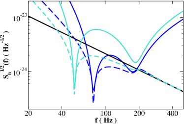
Figure 5: Plot of $\sqrt{S_{h,2}}$ (continuous lines) and $\sqrt{S^{\rm min}_{h,2}}$ (dashed lines) versus frequency $f$ for $T=0.033$, $\epsilon=2\pi\times 25.0\,{\rm Hz}$, $\lambda=2\pi\times 191.3\,{\rm Hz}$, and two different values of the laser power circulating in the arm cavities: $I_{c}=300$ kW (lighter-color lines) and $I_{c}=600$ kW (darker-color lines). The free-mass SQL line (black straight line) is also shown for comparison.

The description of the measurement system in terms of the uncorrelated fields, ${\cal Z}^{\prime}_{i}$ and ${\cal F}^{\prime}_{i}$, yields another way of understanding why in SR interferometers the free mass SQL, $S_{h}^{\rm SQL}\equiv h^{2}_{\rm SQL}$, loses its significance. Indeed, by using Eq. (74), we get $S_{{\cal Z}^{\prime}_{i}{\cal Z}^{\prime}_{i}}=\hbar^{2}/S_{{\cal F}^{\prime}_{i}{\cal F}^{\prime}_{i}}$. Plugging this expression into Eq. (75), minimizing with respect to $S_{{\cal F}^{\prime}_{i}{\cal F}^{\prime}_{i}}$, we obtain,

$$S^{\rm min}_{{\cal F}^{\prime}_{2}{\cal F}^{\prime}_{2}}(\Omega)=\frac{\hbar}{|1+R_{xx}(\Omega)\,K^{\rm eff}_{2}(\Omega)|}\,\frac{1}{R_{xx}(\Omega)}\,,$$ (81)

and the minimal noise spectral density is,

$$S_{h,i}^{\rm min}(\Omega)=\frac{2\hbar}{L^{2}}\,\left|\frac{R^{2}_{xx}(\Omega)}{\chi^{\rm eff}_{i}(\Omega)}\right|=S_{h}^{\rm SQL}\left|\frac{R_{xx}(\Omega)}{\chi_{i}^{\rm eff}(\Omega)}\right|\,,$$ (82)

which can be formally regarded as a non-free-mass SQL for the effective dynamics described by $\chi_{i}^{\rm eff}$. To give an example, in Fig. 5 we plot the square root of the noise spectral densities $S_{h,2}$ and $S^{\rm min}_{h,2}$ versus frequency $f$ having fixed $\epsilon=2\pi\times 25.0\,{\rm Hz}$, $\lambda=2\pi\times 191.3\,{\rm Hz}$, for two different values of the laser power circulating in the arm cavities: $I_{c}=300$ kW and $I_{c}=600$ kW. For comparison we also plot the free-mass SQL line. As we can see from the plot, $S^{\rm min}_{h,2}$ can go quite below the free-mass SQL.

The effective dynamics can be also used to optimize the performance of SR interferometers FK . The roots of the following equation,

$$K^{\rm eff}_{i}(\Omega)-\frac{m}{4}\,\Omega^{2}=0\,,$$ (83)

corresponds to resonances produced by the effective rigidity, at which $\chi^{\rm eff}\rightarrow\infty$ and, using Eq. (82),

$$S_{h,i}^{\rm min}(\Omega)\rightarrow 0\,.$$ (84)

As observed by Khalili FK , we could expect that the more the roots of Eq. (83) coincide, the more broadband the noise curve will be. For example, we could expect that interferometer configurations with double or triple zeros be optimal. However, as we shall see, those configurations are not much better than some of the three-single-zero cases.

Assuming the second quadrature ($i=2$) is observed, we obtain for the triple-zero case [see also Eqs. (29), (30) and (31) in Ref. FK ]:

$$\iota_{c}=2\left(\frac{9\sqrt{177}-113}{49}\right)\,\lambda^{3}\,,\quad\quad\epsilon=\frac{\sqrt{280-21\,\sqrt{177}}}{7}\,\lambda\,,\quad\quad\Omega_{\rm triple\,zero}=\sqrt{\frac{2(-11+\sqrt{177})}{7}}\,\lambda\,.$$ (85)

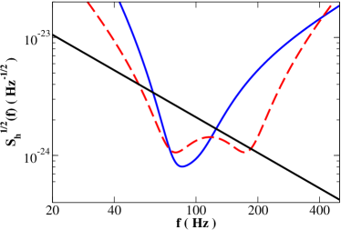
Figure 6: Plot of the square root of the noise spectral density $S_{h}$ versus frequency $f$ for (i) triple-zero case (continuous line) with $\lambda=2\pi\times 123.2\,{\rm Hz}$, $\epsilon=2\pi\times 13.8\,{\rm Hz}$, and $I_{c}=320$ kW and (ii) three-single-zero case (dashed line) with $\lambda=2\pi\times 191.3\,{\rm Hz}$, $\epsilon=2\pi\times 25.0\,{\rm Hz}$ and $I_{c}=590$ kW. For comparison we also show the free-mass SQL line (black straight line).

In Fig. 6 we plot the square root of the noise spectral density $S_{h,2}$ versus frequency $f$ for the triple-zero case having fixed $\Omega_{\rm triple\,zero}=2\pi\times 100$ Hz, i.e. the (free) oscillation frequency $\lambda=2\pi\times 123.3\,{\rm Hz}$ and $\epsilon=2\pi\times 13.8\,{\rm Hz}$. The SQL line is also plotted. For comparison we also show the noise spectral density $S_{h,2}$ corresponding to a solution of Eq. (83) with three-single zeros: $\lambda=2\pi\times 191.3\,{\rm Hz}$, $\epsilon=2\pi\times 25.0\,{\rm Hz}$ and $I_{c}=590$ kW. As mentioned, the spectral density in the triple-zero case is not significantly broad-band, especially if compared with the three-single-zero case.

This result originates from the non-universal nature of the curve $S_{h,i}^{\rm min}$. The SQL (28) does not change if we adjust (by varying the circulating power) the balance between shot noise and radiation-pressure noise and find the interferometer parameters whose noise curve can touch it. By contrast, the curve $S_{h,i}^{\rm min}$ changes when we adjust (by varying the circulating power or the optical resonant frequencies) the effective shot and radiation-pressure noises, $S_{{\cal Z}^{\prime}_{i}{\cal Z}^{\prime}_{i}}$ and $S_{{\cal F^{\prime}}_{i}{\cal F}^{\prime}_{i}}$. [The change of $S_{h,2}^{\rm min}$ as $I_{c}$ is varied can be also seen from Fig. 5.] As a consequence, the fact that $S_{h,i}^{\rm min}$ is low and broad-band for a certain configuration cannot guarantee the noise curve will also be optimal. In particular, in the triple-zero case, Eq. (83) already fixes all the interferometer parameters, leaving no freedom for the noise curve to really take advantage of the triple zeros. The fact that only a non-universal minimum noise spectral density exists in SR interferometers arises in part because of the double role played by the carrier light. Indeed, the latter provides the means for measurement, and therefore determines the balance between shot and radiation-pressure noises, but it also directly affects the optomechanical dynamics of the system, originating the optical-spring effect.

Finally, Braginsky, Khalili and Volikov BKV have recently proposed a table-top quantum-measurement experiment to (i) investigate the ponderomotive rigidity effect present in single detuned cavity and (ii) beat the free mass SQL. Although the table-top experiment will concern physical parameters very different from LIGO-II, e.g., the test mass $m\sim 2\times 10^{-2}$ g, $L\sim 1$ cm, $\Omega\sim 10^{4}\,s^{-1}$, $I_{c}\sim 1\mbox{-}10\,{\rm W}$, however, because of the equivalence we have explicitly demonstrated between SR interferometers and single detuned cavities, the results of the table-top experiment could shed new light and investigate various features of SR optomechanical configurations relevant for LIGO-II.

IV.4 Optical spring equivalent to mechanical spring but at zero temperature

When proposing the optical-bar GW detectors OB , Braginsky, Gorodetsky and Khalili pointed out that detuned optical pumping field in Fabry-Perot resonator can convert the free test mass into an optical spring having very low intrinsic noise. In this section we illustrate why this happens in SR interferometers and why optical springs are indeed preferable to mechanical springs in measuring very tiny forces.

The Heisenberg operator in Fourier domain $x^{(1)}(\Omega)$ describing the antisymmetric mode of motion of SR interferometer, satisfies the following equation [see Eqs. (39), (41) above and also Eq. (2.20) of Ref. BC2 ]:

$$x^{(1)}(\Omega)=\chi(\Omega)\,F^{(0)}(\Omega)\,,\quad\quad\chi(\Omega)=\frac{R_{xx}(\Omega)}{1-R_{xx}(\Omega)\,R_{FF}(\Omega)}\,.$$ (86)

Using Eq. (49) we get:

$$\chi(\Omega)=\frac{4}{m}\,\frac{\lambda^{2}+(\epsilon-i\Omega)^{2}}{\lambda\,\iota_{c}-\Omega^{2}\,[\lambda^{2}+(\epsilon-i\Omega)^{2}]}\,.$$ (87)

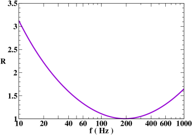
Figure 7: Plot of $R\equiv S_{x}(f)/(2\hbar\,|\Im[\chi(f)]|)$ versus $f$ when $\lambda=2\pi\times 191.3\,{\rm Hz}$, $\epsilon=2\pi\times 25.0\,{\rm Hz}$ and $I_{c}=590$ kW.

The noise spectral density associated with $x$ is:

$$S_{x}(\Omega)=|\chi(\Omega)|^{2}\,S_{F}(\Omega)\,,$$ (88)

where:

$$\pi\,\delta\left(\Omega-\Omega^{\prime}\right)\,S_{x}(\Omega)=\langle 0_{\tilde{a}}|\,x^{(1)}(\Omega)x^{(1)\,\dagger}(\Omega^{\prime})|0_{\tilde{a}}\rangle\,,\quad\quad\pi\,\delta\left(\Omega-\Omega^{\prime}\right)\,S_{F}(\Omega)=\langle 0_{\tilde{a}}|\,F^{(0)}(\Omega)F^{(0)\,\dagger}(\Omega^{\prime})|0_{\tilde{a}}\rangle\,.$$ (89)

More explicitly,

$$S_{F}(\Omega)=\frac{{\cal I}_{c}\,\hbar}{2}\,\frac{\epsilon\,(\lambda^{2}+\epsilon^{2}+\Omega^{2})}{[(\Omega-\lambda)^{2}+\epsilon^{2}]\,[(\Omega+\lambda)^{2}+\epsilon^{2}]}\,.$$ (90)

For the optical spring, which is made up of electromagnetic oscillators in their ground states (the vacuum state), we have [see e.g., Chapter 6 in Ref. BK92  ]:

$$S_{x}(\Omega)\geq 2\hbar\,|\Im[\chi(\Omega)]|\,,$$ (91)

which can be regarded as a zero-temperature version of the fluctuation-dissipation theorem. For a mechanical system, e.g., a mechanical spring, with the same susceptibility, but in thermal equilibrium at temperature $T\gg\hbar\Omega/k$, where $k$ is the Boltzmann constant, the standard version of fluctuation-dissipation theorem says,

$$S_{x}(\Omega)=4\frac{k\,T}{\Omega}\,|\Im[\chi(\Omega)]|\,.$$ (92)

If we assume $\Omega\sim 2\pi\times 100\,{\rm Hz}$, $\hbar\Omega/k\sim 5\times 10^{-9}\,{\rm Kelvin}$, the condition $T\gg\hbar\Omega/k$ is always valid for any practical mechanical system. As a consequence,

$$S_{x}^{\rm mech.\,spring}(\Omega)\sim\frac{k\,T}{\hbar\,\Omega}\,S_{x}^{\rm opt.\,spring}(\Omega)\,.$$ (93)

At $T=300K$, $\Omega/2\pi=100$ Hz, we get $S_{x}^{\rm mech.\,spring}\sim 10^{11}\,S_{x}^{\rm opt.\,spring}$. Thus, because of the very large coefficient $kT/\hbar\Omega$ in Eq. (93), fluctuating noise in an optical spring is always much smaller than in a mechanical spring!

For SR interferometers described in this paper, the fluctuating noise $S_{x}$ does not saturate the inequality in Eq. (91). This can be inferred from Fig. 7 where we plot $R\equiv S_{x}(f)/(2\hbar\,|\Im[\chi(f)]|)$ versus $f$, where $S_{x}$ has been obtained from Eqs. (87), (88) and (90), for the following choice of the physical parameters: $m=30$ kg, $T=0.033$, $\gamma=2\pi\times 98.5\,{\rm Hz}$, with $\lambda=2\pi\times 191.3\,{\rm Hz}$, $\epsilon=2\pi\times 25.0\,{\rm Hz}$ and $I_{c}=560$ kW. The minimum of $R$ is at the frequency corresponding to the (free) oscillation frequency of the SR interferometer, i.e. $f_{\rm min}=\lambda/(2\pi)=191.3$ Hz.

V Input–output relation at all orders in transmissivity of internal test-mass mirrors

To simplify the calculation and the modeling of GW interferometers, KLMTV KLMTV00 calculated the input–output relation of a conventional interferometer at leading order in $T$ and $\Omega\,L/c$. By taking only the leading order terms in $T$, they ignored the radiation-pressure forces acting on the ITM due to the electromagnetic field present in the cavity made up of ITM and BS. By limiting their analysis to the leading order in $\Omega L/c$, they assumed the radiation-pressure forces acting on the ITM and ETM are equal. In conventional interferometers, $T$ alone determines the half-bandwidth $\gamma$ of the arm cavities (through $\gamma=Tc/4L$), which fully characterizes the interferometer [see Eq. (16) in Ref. KLMTV00 and Eqs. (30), (31) above]. Moreover, since $\Omega_{\rm GW}$ is comparable to $\gamma$ and $T\sim 0.005-0.033$, the two small quantities, $\Omega L/c$ and $T$ are on the same order, and the accuracy in expanding the input–output relation in these two parameters is rather under control. [Note that if $\gamma\sim 2\pi\times 100\,{\rm Hz}$, we have $T\sim 0.033$.]

In describing SR interferometers, the authors of Refs. BC1 ; BC2 ; BC3 build on the leading-order results of Ref. KLMTV00 . However, in SR interferometers the accuracy of expanding in $T$ can be quite obscure, because $T$ is not the only small quantity characterizing SR-interferometer performances — for example the SRM transmissivity can also be a small quantity. Thus, to clarify the accuracy of the expansion in $T$, we now derive the input–output relation at all orders in $T$, and compare with the leading order result (24) BC1 ; BC2 . The calculation is much easier if we view the SR cavity as a single effective mirror, as done in Sec. II. However, in doing so, we still use the assumptions mentioned at the beginning of this section. See also the end of Sec. II.1.

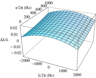
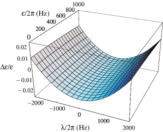
Figure 8: We plot the fractional error $\Delta\lambda/\lambda$ (in left panel) and $\Delta\epsilon/\epsilon$ (in right panel) as a function of $\lambda$ and $\epsilon$. The quantities $\Delta\lambda$ and $\Delta\epsilon$ are the difference between the value of $\lambda$ and $\epsilon$ obtained from the first-order-$T$ free optical frequency (94) and the exact one (13).

V.1 Free optical resonant frequencies

It is interesting to investigate the error in the prediction of the (free) optical resonant frequency introduced by using only the leading order terms in $T$ and $\Omega L/c$. For a generic set of $T$, $\rho$ and $\phi$, it can be quite complicated to characterize that error. For example, when $\rho>\sqrt{R}$ and $\phi\sim\pi/2$, $\widetilde{\rho}^{\prime}$ is near $-1$ (in the complex plane) and the expansion (15) around $\widetilde{\rho}^{\prime}=1$ totally breaks down. However, we are only concerned with those parameters meaningful for a GW detector, and thus we limit our analysis to the region where $|\widetilde{\Omega}|=\sqrt{\lambda^{2}+\epsilon^{2}}\sim\Omega_{\rm GW}<10^{4}\,\mathrm{s}^{-1}$, corresponding to $|\widetilde{\Omega}L/c|\stackrel{{\scriptstyle<}}{{{}_{\sim}}}0.1$. In this way $|\widetilde{\rho}^{\prime}-1|$ is always relatively small. To test the accuracy, we fix $T$, and for each $\widetilde{\Omega}=-\lambda-i\epsilon$, we solve Eq. (13) for $\rho$ and $\phi$. Then, we insert these values into Eq. (17) to get the first-order-$T$ expression for $\widetilde{\Omega}$, which we denote by $\widetilde{\Omega}^{(1)}$. The result is:

$$\widetilde{\Omega}^{(1)} = \frac{c}{L}\,\left(\frac{1+\sqrt{R}}{2}\right)^{2}\,\tan\left(\frac{\widetilde{\Omega}L}{c}\right)\,,$$ (94)

$$= \widetilde{\Omega}\left[1-\frac{T}{2}+{\cal O}(T^{2})\right]\left[1+\frac{1}{3}\left(\frac{\widetilde{\Omega}L}{c}\right)^{2}+{\cal O}\left(\frac{\widetilde{\Omega}^{4}L^{4}}{c^{4}}\right)\right]\,.$$

From this equation we infer that since $|\widetilde{\Omega}L/c|\stackrel{{\scriptstyle<}}{{{}_{\sim}}}0.1$, and $T$ is smaller than a few percents, the error in the (free) optical resonant frequency is not very significant (less than a few percents). In Fig. 8 we plot the fractional differences (denoted by $\Delta\lambda/\lambda$ and $\Delta\epsilon/\epsilon$) between the real and imaginary parts of $\widetilde{\Omega}^{(1)}$ and $\widetilde{\Omega}$, as functions of $\epsilon$ and $\lambda$ for $T=0.033$. The fractional differences are always smaller than $2.5\%$.

V.2 Input–output relation and noise spectral density

Using the formalism of Sec. II and Appendix A, it is rather easy to derive the exact input–output relation in terms of $\lambda$, $\epsilon$ and $\iota_{c}$. The input–output relation ($j$-$k$) of the arm cavity composed of the effective ITM and ETM is:

$$\left(\begin{array}[]{c}k_{1}\\ k_{2}\end{array}\right)=e^{2i\Omega L/c}\left(\begin{array}[]{cc}1&0\\ -{\cal K}_{\rm arm}&1\end{array}\right)\left(\begin{array}[]{c}j_{1}\\ j_{2}\end{array}\right)+e^{i\Omega L/c}\sqrt{2{\cal K}_{\rm arm}}\frac{h}{h_{\rm SQL}^{\rm arm}}\left(\begin{array}[]{c}0\\ 1\end{array}\right)\,,$$ (95)

where

$${\cal K}_{\rm arm}=\frac{8I_{\rm arm}\omega_{0}}{\mu_{\rm arm}\Omega^{2}c^{2}}=\frac{16I_{c}\omega_{0}}{m\Omega^{2}c^{2}}\,,\quad h_{\rm SQL}^{\rm arm}=\sqrt{\frac{8\hbar}{\mu_{\rm arm}\Omega^{2}L^{2}}}=\sqrt{\frac{8\hbar}{m\Omega^{2}L^{2}}}\,.$$ (96)

Writing Eqs. (7) and (8) in terms of quadratures, that is

$$\left(\begin{array}[]{c}{j}_{1}\\ {j}_{2}\end{array}\right)=\sqrt{1-|\widetilde{\rho}^{\prime}|^{2}}\,\left(\begin{array}[]{c}\widetilde{a}_{1}\\ \widetilde{a}_{2}\end{array}\right)+|\widetilde{\rho}^{\prime}|\,\left(\begin{array}[]{cc}\cos\psi&-\sin\psi\\ \sin\psi&\cos\psi\end{array}\right)\,\left(\begin{array}[]{c}{k}_{1}\\ {k}_{2}\end{array}\right)\,,$$ (97)

and

$$\left(\begin{array}[]{c}\widetilde{b}_{1}\\ \widetilde{b}_{2}\end{array}\right)=\sqrt{1-|\widetilde{\rho}^{\prime}|^{2}}\,\left(\begin{array}[]{c}k_{1}\\ k_{2}\end{array}\right)-|\widetilde{\rho}^{\prime}|\,\left(\begin{array}[]{cc}\cos\psi&\sin\psi\\ -\sin\psi&\cos\psi\end{array}\right)\,\left(\begin{array}[]{c}\widetilde{a}_{1}\\ \widetilde{a}_{2}\end{array}\right)\,,$$ (98)

where $\psi={\rm arg}(\widetilde{\rho}^{\prime})$, and using Eq. (11), we obtain the input–output relation ($\widetilde{a}-\widetilde{b}$) of the three-mirror cavity, and thus that of the equivalent SR interferometer. They can be represented in the same form as Eq. (24), with $\widetilde{M}^{(1)}$, $\widetilde{C}_{ij}^{(1)}$, and $\widetilde{D}_{i}^{(1)}$ replaced by:

$$\widetilde{M}^{\rm ex}=\frac{\Omega^{2}c^{2}e^{-2i\Omega L/c}}{4L^{2}}\left\{\left[1-e^{2i(\Omega+\lambda+i\epsilon)L/c}\right]\left[1-e^{2i(\Omega-\lambda+i\epsilon)L/c}\right]+i\frac{\iota_{c}L}{\Omega^{2}c}\left[e^{2i(\Omega+\lambda+i\epsilon)L/c}-e^{2i(\Omega-\lambda+i\epsilon)L/c}\right]\right\}\,,$$ (99)

and

$$\widetilde{C}_{11}^{\rm ex} = \widetilde{C}_{22}^{\rm ex}=\frac{\Omega^{2}c^{2}}{4L^{2}}\left\{\left[1-2e^{-2\epsilon L/c}\cos(2\lambda L/c)\cos(2\Omega L/c)+e^{-4\epsilon L/c}\cos(4\lambda L/c)\right]+\frac{\iota_{c}L}{\Omega^{2}c}e^{-4\epsilon L/c}\sin(4\lambda L/c)\right\}\,,$$ (100)

$$\widetilde{C}_{12}^{\rm ex} = \frac{\Omega^{2}c^{2}}{4L^{2}}\left\{-2e^{-2\epsilon L/c}\sin(2\lambda L/c)\left[\cos(2\Omega L/c)-e^{-2\epsilon L/c}\cos(2\lambda L/c)\right]+\frac{2\iota_{c}L}{\Omega^{2}c}e^{-4\epsilon L/c}\sin^{2}(2\lambda L/c)\right\}\,,$$ (101)

$$\widetilde{C}_{21}^{\rm ex} = \frac{\Omega^{2}c^{2}}{4L^{2}}\left\{2e^{-2\epsilon L/c}\sin(2\lambda L/c)\left[\cos(2\Omega L/c)-e^{-2\epsilon L/c}\cos(2\lambda L/c)\right]-\frac{2\iota_{c}L}{\Omega^{2}c}\left[1-e^{-4\epsilon L/c}\cos^{2}(2\lambda L/c)\right]\right\}\,,$$ (102)

$$\widetilde{D}_{1}^{\rm ex} = \frac{\Omega^{2}c^{2}}{4L^{2}}\left[-2e^{-2\epsilon L/c}e^{i\Omega L/c}\sin(2\lambda L/c)\right]\sqrt{\frac{(1-e^{-4\epsilon L/c})\iota_{c}L}{\Omega^{2}c}}\,,$$ (103)

$$\widetilde{D}_{2}^{\rm ex} = \frac{\Omega^{2}c^{2}}{4L^{2}}\left[2e^{-i\Omega L/c}-2e^{-2\epsilon L/c}e^{i\Omega L/c}\cos(2\lambda L/c)\right]\sqrt{\frac{(1-e^{-4\epsilon L/c})\iota_{c}L}{\Omega^{2}c}}\,.$$ (104)

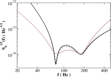
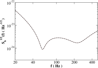
Figure 9: Comparison of first-order $T$-expanded (dashed line) and exact (continuous line) noise spectral density $\sqrt{S_{h}}$ versus frequency $f$. In the left panel we use the parameters $T=0.033$, $\rho=0.9$ and $\phi=\pi/2-0.47$, $m=30\,{\rm kg}$, and $I_{c}=592\,{\rm kW}$ and show the curves for the two orthogonal quadratures $\widetilde{b}_{1}$ (lighter-color lines) and $\widetilde{b}_{2}$ (darker-color lines). In the right panel we use $T=0.005$, $\rho=0.964$, $\phi=\pi/2-0.06$, $m=40\,{\rm kg}$, $I_{c}=840\,{\rm kW}$, and $\zeta=1.13\pi$.

In order to compare with the results obtained in Refs. BC1 ; BC2 ; BC3 , we have also to relate $\widetilde{a}$, $\widetilde{b}$ to $a$ and $b$. The exact transformations [to be compared with Eqs. (22), (23)] are:

$$\left(\begin{array}[]{c}\widetilde{a}_{1}\\ \widetilde{a}_{2}\end{array}\right)=\frac{1}{\sqrt{1+2\rho\sqrt{R}\cos 2\phi+\rho^{2}R}}\left(\begin{array}[]{cc}(1+\rho\sqrt{R})\cos\phi&-(1-\rho\sqrt{R})\sin\phi\\ (1-\rho\sqrt{R})\sin\phi&(1+\rho\sqrt{R})\cos\phi\end{array}\right)\left(\begin{array}[]{c}a_{1}\\ a_{2}\end{array}\right)\,,$$ (105)

and

$$\left(\begin{array}[]{c}\widetilde{b}_{1}\\ \widetilde{b}_{2}\end{array}\right)=\frac{1}{\sqrt{1+2\rho\sqrt{R}\cos 2\phi+\rho^{2}R}}\left(\begin{array}[]{cc}(1+\rho\sqrt{R})\cos\phi&(1-\rho\sqrt{R})\sin\phi\\ -(1-\rho\sqrt{R})\sin\phi&(1+\rho\sqrt{R})\cos\phi\end{array}\right)\left(\begin{array}[]{c}b_{1}\\ b_{2}\end{array}\right)\,.$$ (106)

As an example, we compare in the left panel of Fig. 9 the exact and first-order $T$-expanded noise spectral densities for the two orthogonal quadratures $\widetilde{b}_{1}$ and $\widetilde{b}_{2}$, having fixed $T=0.033$, $\rho=0.9$, $\phi=\pi/2-0.47$, $m=30\,{\rm kg}$ and $I_{c}=592\,{\rm kW}$ (which corresponds to $I_{0}=I_{\rm SQL}$ at BS) as used in Refs. BC1 ; BC2 ; BC3 . The $T$-expanded noise spectral density is given by Eq. (37), where we used for $\lambda$, $\epsilon$ and the redefined output quadratures Eqs. (18), (19). The exact noise spectral density is obtained from Eq. (36) by replacing $\widetilde{M}^{(1)}$, $\widetilde{C}_{ij}^{(1)}$, and $\widetilde{D}_{i}^{(1)}$ with $\widetilde{M}^{\rm ex}$, $\widetilde{C}_{ij}^{\rm ex}$, and $\widetilde{D}_{i}^{\rm ex}$. From Fig. 9, we see that there is a discernible difference. In the right panel of Fig. 9, we compare the exact and first-order $T$-expanded noise spectral densities using the reference-design parameters of LIGO-II LIGOIIref : $T=0.005$, $\rho=0.964$, $\phi=\pi/2-0.06$, $m=40\,{\rm kg}$, $I_{c}=840\,{\rm kW}$, and $\zeta=1.13\pi$. In this case, the two curves agree nicely with each other, presumably, because $T$ is rather small.

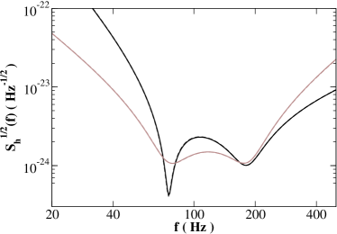
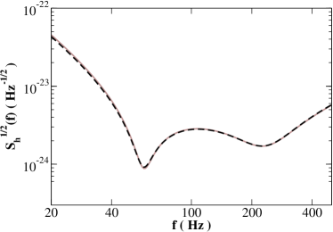
Figure 10: Comparison of first-order $\lambda$-$\epsilon$-$\iota_{c}^{1/3}$-expanded (dashed line) and exact (continuous line) noise spectral density $\sqrt{S_{h}}$ versus frequency $f$. In the left panel we use $T=0.033$, $\rho=0.9$ and $\phi=\pi/2-0.47$, $m=30\,{\rm kg}$, and $I_{c}=592\,{\rm kW}$, and show the curves for the two orthogonal quadratures $\widetilde{b}_{1}$ (lighter-color lines) and $\widetilde{b}_{2}$ (darker-color lines). In the right panel we use $T=0.005$, $\rho=0.964$, $\phi=\pi/2-0.06$, $m=40\,{\rm kg}$, $I_{c}=840\,{\rm kW}$, and $\zeta=1.13\pi$.

In the general case, if we want to trust the leading order calculation, it is not obvious how small $T$ can be, since $\rho$ and $\phi$ have to change along with $T$ to preserve the invariance of interferometer performance. For this reason, it is more convenient to seek an expansion that is also scaling invariant, i.e. whose accuracy only depends on the scaling-invariant properties of the interferometer. To this respect, the set of quantities $\lambda L/c$, $\epsilon L/c$, $\iota_{c}^{1/3}L/c$ and $\Omega L/c$, which are all small and on the same order, is a good choice. It is then meaningful to expand with respect to these quantities and take the leading order terms. We denote the noise spectral density obtained in this way by first-order $\lambda$-$\epsilon$-$\iota_{c}^{1/3}$-expanded noise spectral density. [This technique of identifying and expanding in small quantities of the same order can be very convenient and powerful in the analysis of complicated interferometer configurations, e.g., the speed meter interferometer speedmeter .] Not surprisingly, doing so gives us right away the scaling-invariant input–output relation (24). In the left and right panels of Fig. 10 we compare the exact and first-order $\lambda$-$\epsilon$-$\iota_{c}^{1/3}$-expanded noise spectral densities for the two orthogonal quadratures $\widetilde{b}_{1,2}$, with the same parameters used in Fig. 9, i.e. $T=0.033$, $\rho=0.9$ and $\phi=\pi/2-0.47$, $m=30\,{\rm kg}$, and $I_{c}=592\,{\rm kW}$ (left panel) and $T=0.005$, $\rho=0.964$, $\phi=\pi/2-0.06$, $m=40\,{\rm kg}$, $I_{c}=840\,{\rm kW}$, and $\zeta=1.13\pi$ (right panel). The first-order $\lambda$-$\epsilon$-$\iota_{c}^{1/3}$-expanded noise spectral density is obtained using for $\lambda$, $\epsilon$ and the redefined output quadratures Eqs. (13), (105). The agreement between the exact and first-order $\lambda$-$\epsilon$-$\iota_{c}^{1/3}$-expanded noise spectral densities is much better than the agreement between the exact and $T$-expanded noise spectral densities, given in Fig. 9.

When either $\lambda L/c$, $\epsilon L/c$, $\iota_{c}^{1/3}L/c$ or $\Omega L/c$ is not small enough, the first-order $\lambda$-$\epsilon$-$\iota_{c}^{1/3}$ expansion fails. An interesting example of astrophysical relevance is the configuration with large $\lambda$ and small $\epsilon$, which has narrowband sensitivities centered around a high (optical) resonant frequency. In the left panel of Fig. 11 we compare the first-order $\lambda$-$\epsilon$-$\iota_{c}^{1/3}$-expanded noise spectral density with the exact one, for the two quadratures $\widetilde{b}_{1,2}$ having fixed: $\lambda=2\pi\times 900\,{\rm Hz}$, $\epsilon=20\,{\rm Hz}$, $m=30\,{\rm kg}$ and $I_{c}=600\,{\rm kW}$. Near the lower optomechanical resonant frequency, the first-order $\lambda$-$\epsilon$-$\iota_{c}^{1/3}$ expansion deviates from the exact one by significant amounts. However, it is sufficient to expand up to the second order in $\lambda L/c$, $\epsilon L/c$, $\iota_{c}^{1/3}L/c$ and $\Omega L/c$ to get a much better agreement, as we infer from the right panel of Fig. 11. [The input–output relation expanded at second order is given in Appendix C.]

VI Conclusions

In this paper we showed that, under the assumptions used to describe SR interferometers BC1 ; BC2 ; BC3 , i.e. radiation pressure forces acting on ETMs and ITMs equal, and ETM and ITM motions neglected during the light round-trip time in arm cavities, the SR cavity can be viewed as a single effective (fixed) mirror located at the ITM position. We then explicitly map the SR optical configuration to a three-mirror cavity JM ; MR [see e.g., Sec. II] or even a single detuned cavity FK [see Sec. IV.2]. The mapping has revealed an interesting scaling law present in SR interferometers. By varying the SRM reflectivity $\rho$, the SR detuning $\phi$ and the ITM transmissivity $T$ in such a way that the circulating power $I_{c}$ and the (free) optical resonant frequency (or more specifically its real and imaginary parts $\lambda$ and $\epsilon$) remain fixed [see Eq. (18)], the input–output relation and the optomechanical dynamics remain invariant.

We expressed the input–output relation (24), noise spectral density (36) and all quantities characterizing the optomechanical dynamics, such as the radiation-pressure force (44) and ponderomotive rigidity (49), in terms of the scaling invariant quantities or characteristic parameters. The various formulas are much simpler than the ones obtained in the original description BC1 ; BC2 ; BC3 . The scaling invariant formalism will be certainly useful in the process of optimizing the SR optical configuration of LIGO-II BCM and for investigating advanced LIGO configurations. Moreover, the equivalance we explicitly showed between SR interferometer and single detuned cavity, could also make the table-top experiments of the kind recently suggested in Ref. BKV more relevant to the development of LIGO-II.

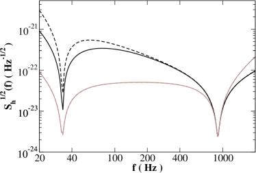
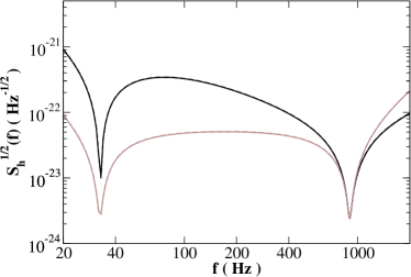
Figure 11: For the two orthogonal quadratures $\widetilde{b}_{1}$ (lighter-color lines) and $\widetilde{b}_{2}$ (darker-color lines) we compare the first-order $\lambda$-$\epsilon$-$\iota_{c}^{1/3}$-expanded noise spectral density (dashed line) with the exact (continuous line) noise spectral density (in left panel) and the second-order $\lambda$-$\epsilon$-$\iota_{c}^{1/3}$-expanded noise spectral density (dashed line) with the exact (continuous line) noise spectral density (in right panel). For all the cases we fix $\lambda=2\pi\times 900\,{\rm Hz}$, $\epsilon=2\pi\times 20\,{\rm Hz}$, $m=30\,{\rm kg}$ and $I_{c}=600\,{\rm kW}$.

In this paper we also evaluated the input–output relation for SR interferometers at all orders in the transmissivity of ITMs [see Sec. V]. So far, the calculations were limited to the leading order. We found that the differences between leading-order and all-order noise spectral densities for broadband configurations of advanced LIGO do not differ much [see Fig. 9]. However for narrowband configurations, which have an astrophysical interest, the differences can be quite noticeable [see left panel of Fig. 11]. In any case, we showed that by using the (very simple) next-to-leading-order input–output relation, explicitly derived in Appendix C, we can recover the all-order results with very high accuracy [see right panel of Fig. 11].

Finally, it will be rather interesting to investigate how the results change if we relax the assumption of disregarding (i) the motion of ITMs and ETMs during the light round-trip time in arm cavities and (ii) the radiation-pressure forces on ITMs due to light power present in the cavity composed of ITM and BS. This analysis is left for future work.

Appendix A Useful relations in the quadrature formalism

As in Refs. KLMTV00 ; BC1 we describe the interferometer’s light by the electric field evaluated on the optic axis, i.e. on the center of light beam. Correspondingly, the electric fields that we write down will be functions of time only. All dependence on spatial position will be suppressed from our formulae.

The input field at the bright port of the beam splitter, which is assumed to be infinitesimally thin, is a carrier field, described by a coherent state with power $I_{0}$ and (angular) frequency $\omega_{0}$. We denote by $f_{\rm GW}=\Omega/2\pi$ the GW frequency, which lies in the range $10-10^{4}$ Hz. The interaction of a gravitational wave with the optical system produces sideband frequencies $\omega_{0}\pm\Omega$ in the electromagnetic field at the dark-port output. We describe the quantum optics inside the interferometer using the two-photon formalism developed by Caves and Schumaker CS85 . The quantized electromagnetic field in the Heisenberg picture evaluated at some fixed point on the optic axis is KLMTV00 ; BC1 :

$$E(t)=\sqrt{\frac{2\pi\hbar\,\omega_{0}}{{\cal A}\,c}}\,e^{-i\omega_{0}\,t}\,\int_{0}^{+\infty}(a_{+}(\Omega)\,e^{-i\Omega t}+a_{-}(\Omega)\,e^{i\Omega t})\,\frac{d\Omega}{2\pi}+{\rm h.c.}\,,$$ (107)

where h.c. means Hermitian conjugate and we denoted $a_{+}(\Omega)\equiv a_{\omega_{0}+\Omega}$ and $a_{-}(\Omega)\equiv a_{\omega_{0}-\Omega}$. Here ${\cal A}$ is the effective cross sectional area of the laser beam and $c$ is the speed of light. The annihilation and creation operators ${a}_{\pm}(\Omega)$ in Eq. (107) satisfy the commutation relations:

$$[a_{+},a_{+^{\prime}}^{\dagger}]=2\pi\,\delta(\Omega-\Omega^{\prime})\,,\quad\quad[a_{-},a_{-^{\prime}}^{\dagger}]=2\pi\,\delta(\Omega-\Omega^{\prime})\,,$$ (108)

$$[a_{+},a_{+^{\prime}}]=0=[a_{-},a_{-^{\prime}}]\,,\quad\quad[a_{+}^{\dagger},a_{+^{\prime}}^{\dagger}]=0=[a_{-}^{\dagger},a_{-^{\prime}}^{\dagger}]\,,\quad\quad[a_{+},a_{-^{\prime}}]=0=[a_{+},a_{-^{\prime}}^{\dagger}]\,.$$ (109)

Following the Caves-Schumaker two-photon formalism CS85 , we introduce the amplitudes of the two-photon modes as

$$a_{1}=\frac{a_{+}+a_{-}^{\dagger}}{\sqrt{2}}\,,\quad\quad a_{2}=\frac{a_{+}-a_{-}^{\dagger}}{\sqrt{2}i}\,;$$ (110)

$a_{1}$ and $a_{2}$ are called quadrature fields and they satisfy the commutation relations:

$$[a_{1},a_{2^{\prime}}^{\dagger}]=-[a_{2},a_{1^{\prime}}^{\dagger}]=2\pi i\delta(\Omega-\Omega^{\prime})\,,$$

$$[a_{1},a_{1^{\prime}}^{\dagger}]=0=[a_{1},a_{1^{\prime}}]\,,\quad\quad[a_{2},a_{2^{\prime}}^{\dagger}]=0=[a_{2},a_{2^{\prime}}]\,.$$ (111)

The electric field (107) in terms of the quadratures reads:

$$E(a_{i};t)=\cos(\omega_{0}\,t)\,E_{1}(a_{1};t)+\sin(\omega_{0}\,t)\,E_{2}(a_{2};t)\,,$$ (112)

where:

$$E_{j}(a_{j};t)=\sqrt{\frac{4\pi\hbar\,\omega_{0}}{{\cal A}\,c}}\,\int_{0}^{+\infty}(a_{j}\,e^{-i\Omega t}+a_{j}^{\dagger}\,e^{i\Omega t})\,\frac{d\Omega}{2\pi}\quad\quad j=1,2\,.$$ (113)

Any linear relation among the fields $a_{\pm}(\Omega)$ of the kind:

$$b_{\pm}{(\Omega)}=f_{\pm}(\Omega)\,a_{\pm}{(\Omega)}\,,\quad\quad f_{+}(\Omega)\equiv f(\omega_{0}+\Omega)\,,\quad\quad f_{-}(\Omega)\equiv f(\omega_{0}-\Omega)\,,$$ (114)

can be transformed into the following relation among the quadrature fields:

$$\left(\begin{array}[]{c}b_{1}\\ b_{2}\end{array}\right)=\frac{1}{2}\left(\begin{array}[]{cc}(f_{+}+f_{-}^{*})&i\,(f_{+}-f_{-}^{*})\\ -i\,(f_{+}+f_{-}^{*})&(f_{+}+f_{-}^{*})\end{array}\right)\left(\begin{array}[]{c}a_{1}\\ a_{2}\end{array}\right)\,.$$ (115)

In general, the above equation can be very complicated. In this paper we restrict ourselves to two special cases. The first case is when $|f_{+}|=|f_{-}|$ and we write

$$f_{\pm}(\Omega)=F(\Omega)\,e^{i\Psi_{\pm}(\Omega)}\,\quad\forall\,\Omega\,>0\,,$$ (116)

and Eq. (115) becomes:

$$\left(\begin{array}[]{c}b_{1}\\ b_{2}\end{array}\right)=F(\Omega)\,e^{i(\Psi_{+}-\Psi_{-})/2}\left(\begin{array}[]{rr}\cos\frac{\Psi_{+}+\Psi_{-}}{2}&-\sin\frac{\Psi_{+}+\Psi_{-}}{2}\\ \sin\frac{\Psi_{+}+\Psi_{-}}{2}&\cos\frac{\Psi_{+}+\Psi_{-}}{2}\end{array}\right)\left(\begin{array}[]{c}a_{1}\\ a_{2}\end{array}\right)\,.$$ (117)

It is easily checked that the input–output relation for the following processes: (i) free propagation in space, (ii) reflection and transmission from a thin mirror, (iii) reflection and transmission from one (or more) Fabry-Perot cavity for which $\omega_{0}$ is either resonant or antiresonant, and (iv) reflection and transmission from one (or more) FP cavity whose bandwidth is much larger than the range of values of $\Omega$ we are interested in [in this case $f(\Omega)$ can be considered as a constant (complex) number] are all special cases (or linear combinations) of the relation (117).

The second case of interest for us is when there is one resonance at $\omega_{0}+\Omega_{\rm r}$, with $\Omega_{\rm r}$ complex. In this case $f(\Omega)$ is of the form:

$$f(\omega)=\frac{g(\omega)}{\omega-\omega_{0}-\Omega_{\rm r}}\,,$$ (118)

where $g(\omega)$ does not have poles. For $\Omega>0$, we have

$$f_{+}=\frac{g(\omega_{0}+\Omega)}{\Omega-\Omega_{\rm r}}\,,\quad\quad f_{-}^{*}=-\frac{g^{*}(\omega_{0}-\Omega)}{\Omega+\Omega^{*}_{\rm r}}\,,$$ (119)

and thus

$$f_{+}+f_{-}^{*} = \frac{(\Omega+\Omega^{*}_{\rm r})\,g(\omega_{0}+\Omega)-(\Omega-\Omega_{\rm r})\,g^{*}(\omega_{0}-\Omega)}{(\Omega-\Omega_{\rm r})\,(\Omega+\Omega^{*}_{\rm r})}\,,$$ (120)

$$f_{+}-f_{-}^{*} = \frac{(\Omega+\Omega^{*}_{\rm r})\,g(\omega_{0}+\Omega)+(\Omega-\Omega_{\rm r})\,g^{*}(\omega_{0}-\Omega)}{(\Omega-\Omega_{\rm r})\,(\Omega+\Omega^{*}_{\rm r})}\,.$$ (121)

Since the quadrature field at $\Omega$ mixes the frequencies $\omega_{0}+\Omega$ and $\omega_{0}-\Omega$, the single resonant frequency $\Omega_{\rm r}$ appears in the above equation as a pair of resonant frequencies $\{\Omega_{\rm r},-\Omega^{*}_{\rm r}\}$.

Appendix B The Stokes relations

The transmission and reflection coefficients of a system of mirrors, or more generally of a two-port linear optical system, can always be expressed in terms of four effective transmissivities and reflectivities: $\widetilde{\rho}$, $\widetilde{\tau}$, $\widetilde{\rho}^{\prime}$ and $\widetilde{\tau}^{\prime}$ [see Fig. 12]. These quantities are generally frequency dependent (complex) numbers. For the fields shown in Fig. 12, we have:

$$j_{\omega} = \widetilde{\rho}^{\prime}k_{\omega}+\widetilde{\tau}a_{\omega}\,,$$ (122)

$$b_{\omega} = \widetilde{\tau}^{\prime}k_{\omega}+\widetilde{\rho}a_{\omega}\,.$$ (123)

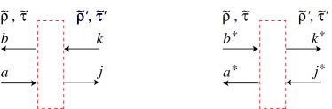
Figure 12: A two-port linear optical system can always be expressed in terms of four effective transmissivities and reflectivities, $\widetilde{\rho}^{\prime}$, $\widetilde{\tau}^{\prime}$ (for fields entering from the right side), and $\widetilde{\rho}$, $\widetilde{\tau}$ (for fields entering from the left side). By taking the complex conjugates of the field amplitudes and inverting their propagation directions, a new set of fields related by the same set of transmissivities and reflectivities is obtained.

Imposing that the two-port linear optical system satisfies the conservation of energy, we have:

$$|\widetilde{\rho}|^{2}+|\widetilde{\tau}|^{2}=1\,,\quad|\widetilde{\rho}^{\prime}|^{2}+|\widetilde{\tau}^{\prime}|^{2}=1\,.$$ (124)

If we take the complex conjugates of all the complex amplitudes and revert their propagation directions, the resulting configuration is also a solution of the optical system, in the sense that the new fields are also related by the same sets of effective transmissivities and reflectivities. Thus, the system is invariant under time reversal. By applying explicitly this symmetry, it is straightforward to derive:

$$\widetilde{\rho}\,\widetilde{\rho}^{*}+\widetilde{\tau}^{\prime}\,\widetilde{\tau}^{*}=1\,,\quad\quad\widetilde{\rho}^{*}\,\widetilde{\tau}+\widetilde{\tau}^{*}\,\widetilde{\rho}^{\prime}=0\,,$$ (125)

$$\widetilde{\rho}^{\prime}\,\widetilde{\rho}^{{}^{\prime}*}+\widetilde{\tau}\,\widetilde{\tau}^{{}^{\prime}*}=1\,,\quad\quad\widetilde{\rho}^{{}^{\prime}*}\,\widetilde{\tau}^{\prime}+\widetilde{\tau}^{{}^{\prime}*}\,\widetilde{\rho}=0\,.$$ (126)

Equations (124)–(126) are the well-known Stokes relations BK . If we rewrite the transmissivity and reflectivity coefficients as

$$\widetilde{\rho}=|\widetilde{\rho}|\,e^{i\mu}\,, \widetilde{\tau}=|\widetilde{\tau}|\,e^{i\nu}\,,$$ (128)

$$\widetilde{\rho}^{\prime}=|\widetilde{\rho}^{\prime}|\,e^{i\mu^{\prime}}\,, \widetilde{\tau}^{\prime}=|\widetilde{\tau}^{\prime}|\,e^{i\nu^{\prime}}\,,$$ (129)

and insert them into the Stokes relations (125)–(126), we obtain

$$|\widetilde{\rho}|=|\widetilde{\rho}^{\prime}|\,,\quad\quad|\widetilde{\tau}|=|\widetilde{\tau}^{\prime}|\,,\quad\quad|\widetilde{\rho}|^{2}+|\widetilde{\tau}|^{2}=1\,;$$ (130)

$$e^{i\nu}=e^{i\nu^{\prime}}\,,\quad\quad e^{i(\mu+\mu^{\prime})}=-e^{2i\nu}\,.$$ (131)

Appendix C Input–output relations at second order in transmissivity of internal test masses

The input–output relation expanded up to second order in $\lambda L/c$, $\epsilon L/c$, $\iota_{c}^{1/3}L/c$ and $\Omega L/c$ can be obtained in a straightforward way by expanding Eqs. (99)–(104). The new coefficients $\widetilde{M}^{(2)}$, $\widetilde{C}^{(2)}_{ij}$ and $\widetilde{D}^{(2)}_{i}$ are very simple. In fact, they can be represented in terms of the first-order ones, $\widetilde{M}^{(1)}$, $\widetilde{C}^{(1)}_{ij}$ and $\widetilde{D}^{(1)}_{i}$ given by Eqs. (25)–(27), through the following formulas (truncated at the next-to-leading order):

$$\widetilde{M}^{(2)}=(1-2\epsilon L/c)\widetilde{M}^{(1)}\,,$$ (132)

$$\left(\begin{array}[]{cc}\widetilde{C}_{11}^{(2)}&\widetilde{C}_{12}^{(2)}\\ \widetilde{C}_{21}^{(2)}&\widetilde{C}_{22}^{(2)}\end{array}\right)=(1-2\epsilon L/c)\left(\begin{array}[]{cc}1&\lambda L/c\\ -\lambda L/c&1\end{array}\right)\left(\begin{array}[]{cc}\widetilde{C}_{11}^{(1)}&\widetilde{C}_{12}^{(1)}\\ \widetilde{C}_{21}^{(1)}&\widetilde{C}_{22}^{(1)}\end{array}\right)\left(\begin{array}[]{cc}1&\lambda L/c\\ -\lambda L/c&1\end{array}\right)\,,$$ (133)

and

$$\left(\begin{array}[]{c}\widetilde{D}_{1}^{(2)}\\ \widetilde{D}_{2}^{(2)}\end{array}\right)=(1-2\epsilon L/c)\left(\begin{array}[]{cc}1&\lambda L/c\\ -\lambda L/c&1\end{array}\right)\left(\begin{array}[]{c}\widetilde{D}_{1}^{(1)}\\ \widetilde{D}_{2}^{(1)}\end{array}\right)\,.$$ (134)

It is quite remarkable that, at second order, the optomechanical resonances, determined by $\widetilde{M}^{(2)}=0$, remain unchanged with respect to the first order result obtained imposing $\widetilde{M}^{(1)}=0$. Apart from a (frequency-independent) rotation of the quadrature phases, the input–output relation at next-to-leading order are very similar to the leading-order one.

References

- (1) A. Abramovici et al., Science 256, 325 (1992); B. Caron et al., Class. Quantum Grav. 14, 1461 (1997); H. Lück et al., Class. Quantum Grav. 14, 1471 (1997); M. Ando et al., Phys. Rev. Lett. 86, 3950 (2001).
- (2) E. Gustafson, D. Shoemaker, K.A. Strain and R. Weiss, “LSC White paper on detector research and development,” LIGO Document Number T990080-00-D, www.ligo.caltech.edu/docs/T/T990080-00.pdf.
- (3) R.W.P. Drever, in The detection of gravitational waves, ed. by D.G. Blair, (Cambridge University Press, Cambridge, England, 1991).
- (4) J.Y. Vinet, B.J. Meers, C.N. Man and A. Brillet, Phys. Rev. D 38, 433 (1998); B.J. Meers Phys. Rev. D 38, 2317 (1998); J. Mizuno et al. Phys. Lett. A 175, 273 (1993); G. Heinzel, “Advanced optical techniques for laser-interferometric gravitational-wave detectors,” Ph.D. thesis, Max-Planck-Institut für Quantenoptik, Garching, 1999.
- (5) K. S. Thorne, “The scientific case for mature LIGO interferometers,” LIGO Document Number P000024-00-R, www.ligo.caltech.edu/docs/P/P000024-00.pdf; C. Cutler and K. S. Thorne, “An overview of gravitational-wave sources,” gr-qc/0204090.
- (6) A. Freise et al. Phys. Lett. A 277, 135 (2000); J. Mason, “Signal Extraction and Optical Design for an Advanced Gravitational Wave Interferometer,” Ph.D. thesis, Caltech, Pasadena, 2001, LIGO document P010010-00-R, www.ligo.caltech.edu/docs/P/P010010-00.pdf.
- (7) H.J. Kimble, Yu. Levin, A.B. Matsko, K.S. Thorne and S.P. Vyatchanin, Phys. Rev. D 65, 022002 (2002).
- (8) A. Buonanno and Y. Chen, Class. Quantum Grav. 18, L95 (2001).
- (9) A. Buonanno and Y. Chen, Phys. Rev. D 64, 042006 (2001).
- (10) A. Buonanno and Y. Chen, Phys. Rev. D 65, 042001 (2002); Class. Quantum Grav. 19 1569 (2002).
- (11) V.B. Braginsky and F.Ya. Khalili, Quantum measurement, edited by K.S. Thorne (Cambridge University Press, Cambridge, England, 1992).
- (12) A. Dorsel, J.D. McCullen, P. Meystre, E. Vignes and H. Walther, Phys. Rev. Lett. 51, 1550 (1983); N. Deruelle and P. Tourrenc, in Gravitation, Geometry and Relativistic Physics (Springer, Berlin, 1984); P. Meystre, E.M. Wright, J.D. McCullen and E. Vignes, J. Opt. Soc. Am. 2, 1830 (1985); J.M. Aguirregabria and L. Bel, Phys. Rev. D 36, 3768 (1988); L. Bel, J.L. Boulanger and N. Deruelle, Phys. Rev. A 7, 37 (1988); B. Meers and N. Mac Donald, Phys. Rev. A 40, 40 (1989); A. Pai, S.V. Dhurandhar, P. Hello and J.Y. Vinet, Europhys. Phys. J. D 8, 333 (2000).
- (13) F.Ya. Khalili, Phys. Lett. A 288, 251 (2001).
- (14) V.B. Braginsky, M.L. Gorodetsky and F.Ya. Khalili, Phys. Lett. A 232, 340 (1997); V.B. Braginsky and F.Ya. Khalili, Phys. Lett. A 257, 241 (1999).
- (15) J. Mizuno, “Comparison of optical configurations for laser-interferometer gravitational-wave detectors,” Ph.D. thesis, Max-Planck-Institut für Quantenoptik, Garching, 1995.
- (16) M. Rachmanov, “Dynamics of laser interferometric gravitational wave detectors,”Ph.D. thesis, Caltech, Pasadena, 2000.
- (17) A.V. Syrtsev and F.Ya. Khalili, JETP 79, 3 1994.
- (18) The reference design of LIGO-II is obtained by optimizing the total noise spectral density, which also includes seismic and thermal noises, with respect to GWs from binary black holes. See www.ligo.caltech.edu/~ligo2/scripts/l2refdes.htmu for details.
- (19) A. Buonanno, Y. Chen and N. Mavalvala (work in progress).
- (20) J.M. Courty, F. Grassia and S. Reynaud, Europhys. Lett. 46, 31 (1999); F. Grassia, J.M. Courty, S. Reynaud and P. Touboul, Eur. Phys. J D 8, 101 (2000).
- (21) V.B. Braginsky, F.Ya. Khalili and P.S. Volikov, Phys. Lett. A 287, 31 (2001).
- (22) P. Purdue, Phys. Rev. D 66, 022001 (2002) ; P. Purdue and Y. Chen, in preparation.
- (23) C.M. Caves and B.L. Schumaker, Phys. Rev. A 31, 3068 (1985); B.L. Schumaker and C.M. Caves, Phys. Rev. A 31, 3093 (1985).
- (24) R. Blandford and K.S Thorne, ”Applications of classical physics,” (unpublished textbook), Chapter 8, www.its.caltech.edu/~rblandfo/ph136/ph136.html.