Irreversible Processes in Inflationary Cosmological Models

Abstract

By using the thermodynamic theory of irreversible processes and Einstein general relativity, a cosmological model is proposed where the early universe is considered as a mixture of a scalar field with a matter field. The scalar field refers to the inflaton while the matter field to the classical particles. The irreversibility is related to a particle production process at the expense of the gravitational energy and of the inflaton energy. The particle production process is represented by a non-equilibrium pressure in the energy-momentum tensor. The non-equilibrium pressure is proportional to the Hubble parameter and its proportionality factor is identified with the coefficient of bulk viscosity. The dynamic equations of the inflaton and the Einstein field equations determine the time evolution of the cosmic scale factor, the Hubble parameter, the acceleration and of the energy densities of the inflaton and matter. Among other results it is shown that in some regimes the acceleration is positive which simulates an inflation. Moreover, the acceleration decreases and tends to zero in the instant of time where the energy density of matter attains its maximum value.

PACS: 98.80.-k; 98.80.Cq

1 Introduction

Cosmological models are among the most important formulations that can be put under analysis when we combine the thermodynamics of irreversible processes with Einstein’s general relativity [1, 2, 3, 4, 5, 6, 7, 8, 9, 10]. Using these theories the different eras of our universe can be modeled; the subject received great attention: the starting point was to consider the hypothesis of homogeneity and isotropy in the form of the Robertson-Walker (RW) metric. More specifically, the early universe physics is of great interest; the so-called inflationary formulations focus on that era, when - according to these models - a rapid expansion of space-time would occur. Using these ideas it is possible to construct a non-equilibrium scenario, where a non-equilibrium pressure term is included in the energy-momentum tensor; this introduces the possibility of creation of particles in the early universe by means of the thermodynamic theory of irreversible processes. In the 3+1 case the inclusion of this term was proposed by Murphy [2] who found a solution that corresponds to a simple expansion. In the inflation driven models a fundamental field, the inflaton, simulates the early universe with an equation of state that will adjust the form of the potential and will affect the temporal evolution of fundamental quantities like the cosmic scale factor and the universe’s energy density.

In this work we start with the Einstein field equations, the inflaton dynamics (in a curved space-time), the conservation law for the energy-momentum tensor, the barotropic equations of state of the inflaton and matter fields. The non-equilibrium pressure is considered as a constitutive quantity - within the framework of ordinary (also known as first order Eckart) thermodynamic theory - which is proportional to the Hubble parameter and whose proportionality factor is identified with the coefficient of bulk viscosity. From these equations we determine the time evolution of the cosmic scale factor, the Hubble parameter, the acceleration and of the energy densities of the inflaton and matter. The evolution equations for these quantities are function of three parameters which are identified with the cosmological constant and two coefficients that appear in the barotropic equations of state for the pressures of the inflaton and of the matter. It is shown that among several possible regimes the acceleration is found to be a positive quantity which simulates an inflation. Moreover, in those regimes the acceleration decreases and tends to zero in the instant of time where the energy density of matter attains its maximum value.

The manuscript is structured as follows. In Section II we introduce the balance equations for the particle four-flow, energy-momentum tensor and entropy four-flow and use the Gibbs equation to identify the non-equilibrium pressure with the process of particle production. We discuss the inflaton equations in Section III and obtain the evolution equation of the energy density of the inflaton as a function of the cosmic scale factor. In Section IV we introduce the Einstein field equations and find a second-order differential equation for the evolution of the cosmic scale factor which is a function of three above mentioned parameters. In Section V we search for the evolution equations of the cosmic scale factor, Hubble parameter, acceleration and of the density energies of the inflaton and matter for given values of the three parameters and initial conditions for the cosmic scale factor and Hubble parameter. Finally, in Section VI we consider the non-equilibrium pressure as a variable within the framework of extended (also known as causal or second-order) thermodynamic theory and discuss the behavior of the solutions. Throughout this paper units have been chosen so that the speed of light $c$ and Planck constant $\hbar$ are equal to one.

2 The Balance Equations

According to the cosmological principle the universe is spatially homogeneous and isotropic so that it looks the same to all observers. These assumptions imply that the universe can be described by the Robertson-Walker metric whose line element in a space-time, characterized by the metric tensor $g_{\mu\nu}$ with signature $(+\,-\,-\,-)$, is given by

$$ds^{2}=dt^{2}-a(t)^{2}\left[{dr^{2}\over 1-kr^{2}}+r^{2}\left(d\theta^{2}+\sin^{2}\theta d\varphi^{2}\right)\right].$$ (1)

In the above equation $a(t)$ is the cosmic scale factor which is an unknown function of the time $t$ and $k$ may assume the values 1, 0, -1 that correspond to closed, flat and open universes, respectively.

We consider that the universe can be modeled as a mixture of two constituents, namely a scalar field and a matter field, in interaction via the gravitational field represented by the cosmic scale factor $a(t)$. There are other ways of modeling this interaction and for more details one is referred to Yokoyama and co-workers [11], Berera [12], Billyard and Coley [13] and the references therein. The scalar field refers to the so-called inflaton [14, 15] and the matter field describes the particles classically. The mixture is characterized by the fields of particle four-flow $N^{\mu}$, energy-momentum tensor $T^{\mu\nu}$ and entropy four-flow $S^{\mu}$ whose balance equations read

$${N^{\mu}}_{;\mu}=n\Sigma,\qquad{T^{\mu\nu}}_{;\nu}=0,\qquad{S^{\mu}}_{;\mu}\geq 0,\qquad$$ (2)

where $n$ denotes the particle number density while $\Sigma$ is the particle production rate.

In a homogeneous and isotropic universe the decompositions of the particle four-flow, energy-momentum tensor and entropy four-flow with respect to the four-velocity $U^{\mu}$ (with $U^{\mu}U_{\mu}=1$) read

$$N^{\mu}=nU^{\mu},\qquad T^{\mu\nu}=(\rho+p+\varpi)U^{\mu}U^{\nu}-(p+\varpi)g^{\mu\nu},\qquad S^{\mu}=nsU^{\mu},$$ (3)

since in this case the stress tensor, the heat flux and the entropy flux vanish. In (3) $\rho$, $p$ and $s$ represent the energy density, the pressure and the entropy per particle of the mixture, respectively. The term $\varpi$ denotes the dynamic pressure which refers to a non-equilibrium pressure; this quantity also represents the production of particles phenomenologically [16]. For this particular case the Eckart and the Landau and Lifshitz decompositions (see for example [17]) coincide.

Insertion of the representations (3) into the balance equations ${N^{\mu}}_{;\mu}=n\Sigma$, $U_{\mu}{T^{\mu\nu}}_{;\nu}=0$, and ${S^{\mu}}_{;\mu}\geq 0$ lead to

$$\dot{n}+n\Theta=n\Sigma,\qquad\dot{\rho}+(\rho+p+\varpi)\Theta=0,\qquad n\dot{s}+ns\Sigma\geq 0,$$ (4)

which represent the balance equations for the particle number density, energy density and entropy density, respectively. In these equations we have introduced the usual notations: $\Theta\equiv{U^{\mu}}_{;\mu}$ for the expansion rate and $\dot{n}\equiv U^{\mu}n_{;\mu}$ for the covariant derivative along $U^{\mu}$.

In terms of the the covariant derivative along $U^{\mu}$ the Gibbs equation reads

$$n\dot{s}={1\over T}\left(\dot{\rho}-{\rho+p\over n}\dot{n}\right),$$ (5)

where $T$ is the absolute temperature. If we eliminate from the Gibbs equation the derivatives of the particle number density $\dot{n}$ and of the energy density $\dot{\rho}$ by using the two first balance equations given in (5) we get

$$n\dot{s}+ns\Sigma={1\over T}\left(-\varpi\Theta-n\mu\Sigma\right)\geq 0,$$ (6)

where $\mu=(\rho+p)/n-Ts$ is the chemical potential.

An adiabatic process is characterized by the requirement that $\dot{s}=0$ so that we can infer from (6) the inequality $ns\Sigma\geq 0$. As was pointed out by Prigogine et al [18] the process of particle production leads to a non-symmetric relationship between space-time and matter since it refers to an irreversible process of particle production due to the gravitational energy. Moreover, we get from (6) when $\dot{s}=0$ that

$$\varpi=-(\rho+p){\Sigma\over\Theta}.$$ (7)

Hence, the dynamic pressure $\varpi$ can be identified with the particle production rate $\Sigma$. This result was first obtained, to the best of our knowledge, by Zimdahl [16].

We write the energy density and the pressure of the mixture as a sum of two terms that describe the scalar and the matter fields, e. g.,

$$\rho=\rho_{\phi}+\rho_{m},\qquad p=p_{\phi}+p_{m},$$ (8)

where $\rho_{\phi}$, $p_{\phi}$, and $\rho_{m}$, $p_{m}$ represent the energy density and the pressure of the inflaton and of the particles, respectively. In this case the energy-momentum tensor for the mixture reads

$$T^{\mu\nu}=(\rho_{\phi}+\rho_{m}+p_{\phi}+p_{m}+\varpi)U^{\mu}U^{\nu}-(p_{\phi}+p_{m}+\varpi)g^{\mu\nu}.$$ (9)

From this point on we shall consider a comoving frame where the four-velocity is given by $(U^{\mu})=(1,{\bf 0})$. In this circumstance the expansion rate is given by $\Theta\equiv 3H$ - where $H=\dot{a}/a$ is the Hubble parameter - and the balance equation $U_{\mu}{T^{\mu\nu}}_{;\nu}=0$ can be written as

$$\dot{\rho}_{\phi}+\dot{\rho}_{m}+3H(\rho_{\phi}+\rho_{m}+p_{\phi}+p_{m}+\varpi)=0.$$ (10)

In a comoving frame the dot reduces to a differentiation with respect to the time.

3 The Inflaton Equations

Modern inflationary theories require the presence of the inflaton. This hypothetical particle is represented classically by a scalar field of the same name and the motivation behind these ideas can be found in the works  [14, 15, 19, 20, 21]. The corresponding Lagrangian density (in a generic curved space-time) for the scalar field $\phi(x^{\mu})$ is written as

$${\cal L}={1\over 2}\partial_{\mu}\phi\partial^{\mu}\phi-V(\phi),$$ (11)

where $V(\phi)$ is the potential density of the field. From the Euler-Lagrange equations of motion one can obtain the dynamics of a homogeneous scalar field

$$\ddot{\phi}+3H\dot{\phi}+{dV(\phi)\over d\phi}=0.$$ (12)

If we consider the inflaton as a perfect fluid with an energy-momentum tensor of the form $(T^{\mu\nu}_{\phi})={\rm diag}(\rho_{\phi},p_{\phi},p_{\phi},p_{\phi})$, we can equate this formula to the expression coming from Noether theorem

$$T^{\mu\nu}_{\phi}=\partial^{\mu}\phi\partial^{\nu}\phi-{\cal L}g^{\mu\nu},$$ (13)

and obtain the equations for the energy density and for the pressure in terms of the homogeneous scalar field, which are given by

$$\rho_{\phi}={1\over 2}\dot{\phi}^{2}+V(\phi),\qquad p_{\phi}={1\over 2}\dot{\phi}^{2}-V(\phi).$$ (14)

We differentiate (14)₁ with respect to the time, make use of (12) and get the following evolution equation for the energy density of the inflaton

$$\dot{\rho}_{\phi}+3H(\rho_{\phi}+p_{\phi})=0.$$ (15)

Equations (10) and (15) show that the energy densities of the inflaton and of the matter decouple so that we can write

$$\dot{\rho}_{m}+3H(\rho_{m}+p_{m}+\varpi)=0.$$ (16)

Now we follow the work of Ratra and Peebles [19] and suppose that the pressure of the inflaton is connected with its energy density according to the barotropic equation of state

$$p_{\phi}=(\nu-1)\rho_{\phi},\qquad\hbox{where}\qquad 0\leq\nu\leq 1.$$ (17)

As we said before, in this model the homogeneous scalar field does not interact with other non-gravitational fields [19].

We insert (17) into (15) and get by integration a relationship between the energy density and the cosmic scale factor

$${\rho_{\phi}\over\rho_{\phi}^{0}}=\left({a_{0}\over a}\right)^{3\nu},$$ (18)

where $\rho_{\phi}^{0}$ and $a_{0}$ are the values of the energy density of the inflaton and of the cosmic scale factor at $t=0$ (by adjusting clocks), respectively. The relationship between the potential density of the scalar field and the cosmic scale factor can be obtained from (14), (17) and (18) yielding

$$V=\rho_{\phi}^{0}\left({2-\nu\over 2}\right)\left({a_{0}\over a}\right)^{3\nu}.$$ (19)

The above result is in agreement with the work of Ratra and Peebles [19] as expected.

Once the time evolution of the cosmic scale factor is known it is possible to obtain from (18) and (19) the time evolution of the energy density and of the potential density of the scalar field. The determination of the cosmic scale factor from the Einstein field equations will be the subject of the next section.

4 Einstein Field Equations

From Einstein field equations

$$R_{\mu\nu}-{1\over 2}Rg_{\mu\nu}=-{8\pi\over m_{\rm P}^{2}}T_{\mu\nu},$$ (20)

where $m_{\rm P}=1/\sqrt{G}$ denotes the Planck mass, $R_{\mu\nu}$ the Ricci tensor and $R$ the curvature scalar, one can get (working with the RW metric) a system of equations that reads

$${\ddot{a}\over a}=-{4\pi\over 3m_{\rm P}^{2}}(\rho_{\phi}+\rho_{m}+3p_{\phi}+3p_{m}+3\varpi),$$ (21)

$$H^{2}+{k\over a^{2}}={8\pi\over 3m_{\rm P}^{2}}(\rho_{\phi}+\rho_{m}).$$ (22)

The system of equations (10), (21) and (22) is not linearly independent, since the differentiation of (22) with respect to the time, taking into account the conservation law (10) leads to (21).

Let us first analyze the case that correspond to a false vacuum where $\nu=0$ so that $p_{\phi}=-\rho_{\phi}=-\rho_{\phi}^{0}$. In this case we have only the scalar field, i. e., the matter field is absent ($\rho_{m}=0$) and it follows from (22)

$$\left({\dot{a}\over a}\right)^{2}+{k\over a^{2}}={8\pi\rho_{\phi}^{0}\over 3m_{\rm P}^{2}}\equiv\chi,$$ (23)

where $\chi$ can be identified with the cosmological constant $\Lambda\equiv 3\chi$. Equation (23) leads to the de Sitter exponential solution $a=a_{0}\exp\left(\sqrt{\chi}\,t\right)$ if one neglects the term $k/a^{2}$ during the rapid expansion.

For $\nu\neq 0$ we can get from (22) together with (10)

$$\dot{H}={k\over a^{2}}-{4\pi\over m_{\rm P}^{2}}(\rho_{\phi}+\rho_{m}+p_{\phi}+p_{m}+\varpi).$$ (24)

In order to determine the time evolution of the cosmic scale factor from (24) one has to know the relationship between the pressure $p_{m}$ and the energy density $\rho_{m}$ of the matter and the constitutive equation for the dynamic pressure $\varpi$, since $p_{\phi}=(\nu-1)\rho_{\phi}$ and the energy density of the scalar field $\rho_{\phi}$ is given by (18). Here we follow the works [2, 10] and write

$$p_{m}=(\gamma-1)\rho_{m},\qquad 1\leq\gamma\leq 2,$$ (25)

$$\varpi=-3\eta H,\qquad\eta=\alpha(\rho_{\phi}+\rho_{m}).$$ (26)

Equation (25) is the barotropic equation of state for the matter and some values for $\gamma$ are: a) dust $\gamma=1$; b) radiation $\gamma=4/3$; c) non-relativistic matter $\gamma=5/3$ and d) stiff matter (or Zel’dovich fluid [4]) $\gamma=2$. Equation (26) relates the dynamic pressure $\varpi$ with the Hubble parameter $H$. The proportionality factor $\eta$ is the coefficient of bulk viscosity which is supposed to be proportional to the energy density of the mixture $\rho=\rho_{\phi}+\rho_{m}$. Moreover, $\alpha$ is a constant.

The evolution equation for the cosmic scale factor is obtained from (24) together with (18), (25) and (26) yielding

$$\dot{H}={k\over a^{2}}-{3\over 2}\left[(\nu-\gamma)\chi\left({a_{0}\over a}\right)^{3\nu}+(\gamma-3\alpha H)\left(H^{2}+{k\over a^{2}}\right)\right].$$ (27)

The above equation is a function of four parameters - namely $\nu$, $\chi$, $\gamma$ and $\alpha$ - for a given value of $k$. We can express one of these parameters as a function of the others. Indeed if we consider that at $t=0$ (by adjusting clocks) we have $H(0)=H_{0}$, $\rho_{m}(0)=0$ and $a(0)=a_{0}$ it follows from (22) and (27)

$$H_{0}^{2}+{k\over a_{0}^{2}}=\chi,\qquad\alpha={3\nu\chi a_{0}^{2}-2k\over 9H_{0}\chi a_{0}^{2}}.$$ (28)

Now we make use of the relationships (28) and get from (27)

$$\dot{H}={k\over a^{2}(\chi-k)}-{3\over 2}\left(\gamma-{3\nu\chi-2k\over 3\chi}H\right)\left(H^{2}+{k\over a^{2}(\chi-k)}\right)$$

$$-{3\over 2}(\nu-\gamma){\chi\over\chi-k}\left({1\over a}\right)^{3\nu},$$ (29)

by introducing the dimensionless quantities: a) a new Hubble parameter $H\equiv H/H_{0}$; b) a new proper time $t\equiv tH_{0}$; c) a new cosmological constant $\chi\equiv\chi a_{0}^{2}$ and d) a new cosmic scale factor $a\equiv a/a_{0}$. Equation (29) is a second-order differential equation for the cosmic scale factor which is a function of three parameters: the cosmological constant $\chi$, and the two coefficients that appear in the barotropic equations of state for the inflaton $\nu$ and matter $\gamma$.

In terms of the dimensionless quantities the energy densities read

$${\rho_{\phi}\over\rho_{\phi}^{0}}=\left({1\over a}\right)^{3\nu},\qquad{\rho_{m}\over\rho_{\phi}^{0}}={\chi-k\over\chi}\left(H^{2}+{k\over a^{2}(\chi-k)}\right)-\left({1\over a}\right)^{3\nu}.$$ (30)

The above equations connect the evolution of the energy densities with the evolution of the cosmic scale factor. In the next section we analyze the time evolution of these quantities for flat, closed and open universes ($k=0,\pm 1$) and for given values of the parameters $\nu$, $\chi$ and $\gamma$.

5 Results and Discussions

In order to obtain the time evolution of the cosmic scale factor and of the energy densities from equations (29) and (30) one has to specify two initial conditions, since (29) is a second-order differential equation for $a(t)$. Here we choose that at the instant of time $t=0$ (by adjusting clocks) the energy density of the inflaton has its maximum value while the energy density of the matter attains its minimum value, namely $\rho_{\phi}(0)=\rho_{\phi}^{0}=1$ and $\rho_{m}(0)=0$. According to (30) these initial conditions are equivalent to fix the value $a(0)=1$ for the cosmic scale factor and $H(0)=1$ for the Hubble parameter. There is still much freedom to find the solutions, since (29) and (30) do depend on the three parameters $\nu$, $\chi$ and $\gamma$ for each kind of universe, i. e., closed, open and flat. Among several possible regimes which can be found by choosing different values for the parameters $\nu$, $\chi$ and $\gamma$ we fix our attention to those values which simulate an inflation - i. e., where the acceleration is a positive quantity - and where the energy of the matter attains its maximum value at the instant of time where the period of the inflation ends - which corresponds to a vanishing acceleration. For a closed universe $(k=1)$ one set of values that satisfies the above mentioned conditions are $\nu=0.9$, $\gamma=1.9$ and $\chi=2.0$. In figures 1 and 2 we have also chosen the same values for a flat $(k=0)$ and open $(k=-1)$ universes in order to compare the different solutions.

In Fig. 1 it is plotted the cosmic scale factor $a$, its velocity $\dot{a}$ and acceleration $\ddot{a}$ as a function of time for closed, flat and open universes. We infer from the curves that an open universe evolves more rapidly than the two other types of universe, while a closed universe evolves more slowly. The same conclusion can be draw out for the acceleration, since the curves show that the inflation period of an open universe is the largest following the flat and the closed universes. We have plotted in Fig. 2 the energy densities of the inflaton and of the matter as function of time. We note from this figure that the energy density of the matter grows more rapidly with respect to the time for an open universe following the cases of flat and closed universes. Moreover, we can infer that the energy density of the inflaton decays more slowly with respect to the time for a closed universe following the cases of flat and open universes. Once the maximum of the energy density of the matter is attained other models should be considered for the universe, since the universe reheats and follows the standard big-bang model.

One may wonder from Fig. 2 why the sum of the energy densities of the inflaton and of the matter is not a constant. This can be explained as follows: in the presence of gravitational fields the energy-momentum tensor of the matter alone does not lead to a conservation law (see for example Landau and Lifshitz [22] and Dirac [23]), since one has to include the energy-momentum pseudo tensor of the gravitational field $T^{\mu\nu}_{G}$ which is given by

$$T^{\mu\nu}_{G}={m_{\rm P}^{2}\over 16\pi}\left[{g^{\mu\tau}\over\sqrt{g}}(\Gamma^{\nu}_{\alpha\beta}-\delta_{\beta}^{\nu}\Gamma^{\sigma}_{\alpha\sigma}){\partial g^{\alpha\beta}\sqrt{g}\over\partial x^{\tau}}-g^{\alpha\beta}(\Gamma^{\sigma}_{\alpha\beta}\Gamma^{\tau}_{\sigma\tau}-\Gamma^{\rho}_{\alpha\sigma}\Gamma^{\sigma}_{\beta\rho})g^{\mu\nu}\right],$$ (31)

where $\Gamma^{\rho}_{\alpha\sigma}$ are Christoffel symbols and $g\equiv-\det(g_{\mu\nu})$.

For a RW metric with $k=0$ we get

$$T^{00}_{G}=-{3m_{\rm P}^{2}\over 8\pi}\left({\dot{a}\over a}\right)^{2},$$ (32)

hence giving the ”expected” relation $T^{00}_{G}+T^{00}_{\phi}+T^{00}_{m}=0$ thanks to $T^{00}_{\phi}=\rho_{\phi}$, $T^{00}_{m}=\rho_{m}$ and (22). One may say that the energy density of the matter increases at the expense of the inflaton and gravitational energies. This result must be handled with care since the energy density of the gravitational field is an intrinsically non-covariant quantity [22, 23].

6 Final Remarks

In this work we have analyzed the irreversible processes within the framework of ordinary thermodynamics instead of extended thermodynamics (see for example [3, 5, 6, 7, 8, 9]). The reason is that - apart from causality - there exist some thermodynamic systems in which ordinary and extended thermodynamics lead to the same results, like the problems concerning the propagation of low frequency waves in fluids and those related to the flow and the heat transfer in fluids in the continuum regime (see for example [24]). When the behavior of the thermodynamic fields are not smooth enough, there exist differences between the solutions of ordinary and extended thermodynamics. Here we confirm that both descriptions can lead to the same behavior of the solutions and for this purpose let us proceed to analyze the same problem by using extended thermodynamics.

In extended thermodynamics the dynamic pressure $\varpi$ is no more given by the constitutive equation (26) but it is a variable whose evolution equation in a linearized theory reads (see for example [17, 24])

$$\varpi+\tau\dot{\varpi}=-3\eta H,$$ (33)

where $\tau$ is a characteristic time. The evolution equations for the heat flux and pressure tensor are not consider here, since we are dealing with a homogeneous and isotropic universe. Hence we have to solve the system of evolution equations for the cosmic scale factor (24) and for the dynamic pressure (33).

According to the kinetic theory of relativistic gases (see for example [17]) the characteristic time which appears in the evolution equation for the dynamic pressure is given by $\tau=\eta/p$, where $p$ is the pressure of the mixture. Hence the system of equations (24) and (33) can be written in terms of dimensionless quantities as

$$\dot{H}-{k\over a^{2}(\chi-k)}+{3\over 2}\left[{(\nu-\gamma)\chi\over\chi-k}\left({1\over a}\right)^{3\nu}+\gamma\left(H^{2}+{k\over a^{2}(\chi-k)}\right)+\varpi\right]=0,$$ (34)

$$\alpha(\chi-k)\dot{\varpi}+\left[\varpi+3\alpha H\left(H^{2}+{k\over a^{2}(\chi-k)}\right)\right]\left[(\nu-\gamma)\chi\left({1\over a}\right)^{3\nu}\right.$$

$$\left.+(\gamma-1)(\chi-k)\left(H^{2}+{k\over a^{2}(\chi-k)}\right)\right]=0,$$ (35)

by introducing the dimensionless quantities $\alpha\equiv\alpha H_{0}$ and $\varpi\equiv 8\pi\varpi/(3m_{\rm P}^{2}H_{0}^{2})$, apart from those defined in Sec. IV.

As we have pointed out in previous sections there exist several possible regimes that can be found by solving the system of equations (34) and (35), since it is a function of four parameters $\nu$, $\chi$, $\gamma$ and $\alpha$. If one chooses the following initial conditions $a(0)=1$, $H(0)=1$ and $\dot{\varpi}(0)=0$ one may obtain for (say) $\nu=0.9$, $\chi=2.0$, $\gamma=1.9$, $\alpha=0.1$ and $k=1$ a solution for the fields in extended (causal) thermodynamics which have the same behavior as those represented in Figs. 1 and 2 by using ordinary (Eckart) thermodynamics.

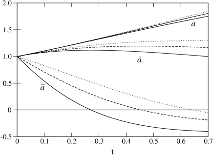
Figure 1: Cosmic scale factor $a$, velocity $\dot{a}$ and acceleration $\ddot{a}$ vs time $t$ for open $k=-1$ (dot-line), flat $k=0$ (dash-line) and closed $k=1$ (straight-line) universes.

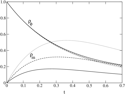
Figure 2: Inflaton energy density $\rho_{\phi}$ and matter energy density $\rho_{m}$ vs time $t$ for open $k=-1$ (dot-line), flat $k=0$ (dash-line) and closed $k=1$ (straight-line) universes.

References

- [1] S. Weinberg, Gravitation and cosmology. Principles and applications of the theory of relativity (Wiley, New York, 1972).
- [2] G. L. Murphy, Phys. Rev. D 8, 4231 (1973).
- [3] V. A. Belinskiǐ, E. S. Nikomarov and I. M. Khalatnikov, Sov. Phys. JETP 50, 213 (1979).
- [4] Ø. Grøn, Astrophys. Space Sci. 173, 191 (1990).
- [5] V. Romano and D. Pavón, Phys. Rev. D 47, 1396 (1993).
- [6] A. A. Coley and R. J. van den Hoogen, Class. Quant. Grav. 12, 1977 (1995).
- [7] R. J. van den Hoogen and A. A. Coley, Class. Quant. Grav. 12, 2335 (1995);
- [8] W. Zimdahl, Phys. Rev. D 61, 083511 (2000).
- [9] A. Di Prisco, L. Herrera and J. Ibáñez, Phys. Rev. D 63, 023501 (2000).
- [10] G. M. Kremer and F. P. Devecchi, Phys. Rev. D 65, 083515 (2002).
- [11] J. Yokoyama, K. Sato and H. Kodama, Phys. Lett. B 196, 129 (1987); J. Yokoyama and K. Maeda, Phys. Lett. B 207, 31 (1988).
- [12] A. Berera, Phys. Rev. Lett. 75, 3218 (1995).
- [13] A. P. Billyard and A. A. Coley, Phys. Rev. D 61, 083503 (2000).
- [14] A. Albrecht, P. J. Steinhardt, M. S. Turner and F. Wilczek, Phys. Rev. Lett. 48, 1437 (1982).
- [15] A. Linde, Particle physics and inflationary cosmology (Harwood Academic Publishers, Chur, 1990).
- [16] W. Zimdahl, Phys. Rev. D 57, 2245 (1998).
- [17] C. Cercignani and G. M. Kremer, The relativistic Boltzmann equation: theory and applications (Birkhäuser, Basel, 2002).
- [18] I. Prigogine, J. Geheniau, E. Gunzig and P. Nardone, Gen. Relat. Grav. 21, 767 (1989).
- [19] B. Ratra and P. J. E. Peebles, Phys. Rev. D 37, 3406 (1988).
- [20] A. R. Lidddle, in High energy physics and cosmology ed. A. Masiero, G. Senjanovic and A. Smirnov, (World Scientific, Singapore, 1999).
- [21] A. H. Guth, Phys. Rep. 333, 555 (2000).
- [22] L. Landau and E. M. Lifshitz, The classical theory of fields 4th ed. (Pergamon Press, New York, 1989).
- [23] P. A. M. Dirac, General theory of relativity (Princeton UP, Princeton, 1996).
- [24] I. Müller and T. Ruggeri, Rational extended thermodynamics (Springer, New York, 1998).