Degeneracy in exotic gravitational lensing

Abstract

We present three different theoretically foreseen, but unusual, astrophysical situations where the gravitational lens equation ends up being the same, thus producing a degeneracy problem. These situations are (a) the case of gravitational lensing by exotic stresses (matter violating the weak energy condition and thus having a negative mass, particular cases of wormholes solutions can be used as an example), (b) scalar field gravitational lensing (i.e. when considering the appearance of a scalar charge in the lensing scenario), and (c) gravitational lensing in closed universes (with antipodes).The reasons that lead to this degeneracy in the lens equations, the possibility of actually encountering it in the real universe, and eventually the ways to break it, are discussed.

I Introduction

Gravitational lensing (GL) has long been advocated as an important tool in studying the Universe. It can act as a cosmic telescope, magnifying distant objects otherwise too dim to be detected. It is also an appropriate avenue to look for the detection of exotic objects in the universe. Unfortunately, initial hopes that GL would be able to resolve many long standing problems (e.g. finding out the value of the Hubble constant through the time delay between the images, or giving an independent estimate of the masses of celestial bodies) went down as it was discovered that GL is subject to degeneracy and is highly model dependent. For example, when statistics of gravitational lensing was first introduced, it was hoped that the dependence of the image separations on the redshift of the source could constitute a test of the curvature of the universe statistics . However, the large systematic and statistical uncertainties, involved with both the observed and predicted number of lensed arcs, as well as the rather small number of the multiply image systems available, do not allow us to constrain cosmological parameters based on current observations, nor even strongly favor one cosmological model above another waga ; antipode ; Cooray99 .

An apparently unique feature of any lens model is its lens equation. Given a class of matter distribution, one can write a corresponding lens equation and solving it (when possible), find all necessary properties of a particular lens. In this work we present three different theoretically foreseen astrophysical situations possessing the same form of the lens equation. The degeneracy is presented among three cases: the exotic lens (understood as a lens made up of matter violating the weak energy condition), the lens endowed with scalar charge, and the case of a closed universe with a source behind the first antipode. We present the details of the resulting images configurations, the reasons leading to the degeneracy, and discuss some ways to get around it.

II Cases

II.1 Exotic lens

An exotic lens is a lens made up of matter violating the weak energy condition (WEC). Existence of such matter admits existence of negative energy densities—and so negative masses. Negative masses within General Relativity have been studied since Bondi’s paper BONDI , but recent attention was regained when wormhole solutions were presented motho ; visser-book .

The detailed treatment of lensing properties of a point negative mass was presented in STR (hereafter STR), for related studies see references therein. Here we will briefly describe the relevant features. If $b$ is the impact parameter of the unperturbed light ray, the deflection angle for a negative point mass lens is ${\bm{\alpha}}_{\rm d}=-4G|M|{\bf b}/c^{2}b^{2}$ and the lens equation is 

$$\beta=\theta+\frac{4G|M|}{c^{2}}\frac{D_{\rm LS}}{D_{\rm S}D_{\rm L}\theta}\,\,.$$ (1)

Defining a useful angular scale in this problem, which in case of ordinary lensing is called an Einstein angle,

$$\theta_{\rm E}^{2}=\frac{4G|M|}{c^{2}}\frac{D_{\rm LS}}{D_{\rm S}D_{\rm L}}\,\,,$$ (2)

we rewrite the lens equation as $\beta=\theta+\theta_{\rm E}^{2}/\theta$. It can be solved to obtain two solutions for the image position $\theta$: $\theta_{1,2}=\frac{1}{2}\left(\beta\pm\sqrt{\beta^{2}-4\theta_{\rm E}^{2}}\right)$. Unlike in the lensing due to positive masses, three distinct regimes appear here: a) $\beta<2\theta_{\rm E}$. There is no real solution for the lens equation—no images when the source is inside $2\theta_{\rm E}$; b) $\beta>2\theta_{\rm E}$. There are two solutions, corresponding to two images on the same side of the lens. One is always inside the angle $\theta_{\rm E}$, the other is always outside it; c) $\beta=2\theta_{\rm E}$. This is a degenerate case, $\theta_{1,2}=\theta_{\rm E}$; two images merge at the $\theta_{\rm E}$ angular radius, forming the radial arc.

Two important scales in this case are the angle $\theta_{\rm E}$— the angular radius of the radial critical curve (RCC), and the angle $2\theta_{\rm E}$—the angular radius of the caustic. When the source crosses the caustic, the two images merge on the critical curve ($\theta_{\rm E}$) and disappear. We do not obtain a tangential critical curve (TCC)—in other words, no Einstein ring is possible and, accordingly, no tangential arcs.

II.2 Scalar fields

With increased interest in string theory, scalar fields, both minimally and conformally coupled to gravity, have been the subject of intensive research in recent years. Several possible astrophysical relevant features of scalar fields have been described. Among them the so-called ‘spontaneous scalarization’ phenomenon damour-WHINNET , the scalar field origin of dark matter on galactic (e.g. Guzman ) and cosmological scales (e.g. Cho ), quintessence (e.g. Fara ), the possible existence of supermassive scalar objects in centers of galaxies TORRES-GAL , and, finally, the scalar field itself acting as a gravitational lens Vir ; Matos ; FRANZ .

One of the solutions to the Einstein-Massless Scalar field (EMS) equations derived for gravity minimally coupled to a scalar field is Janis-Newman-Winicour’s (JNW) JANIS . It describes the exterior of a static, spherically symmetric, and singular, massive object, endowed with the usual Schwarzschild mass $M$ and a so-called scalar charge $q$—the signature of the conformal coupling of the massless scalar field with gravitation. The “scalar charge” does not contribute to the total mass of the system, but it does affect the curvature of the spacetime vir97 . The JNW solution also describes the space-time due to a naked singularity. The difference between these two objects lies in the value of a parameter $b$, which is defined as the curvature singularity ($b<r<\infty$, where $r$ is the radial coordinate of the JNW metric). When the radius of the object is greater than $b$, the lens is extended, spherically symmetric and static. When $r=b$, it is a naked singularity Vir .

The deflection angle (up to the second order) for the JNW metric is given by

$$\alpha_{\rm d}(r_{0})=\frac{4m}{r_{0}}+\frac{4m^{2}}{r_{0}^{2}}\left(\frac{15\pi}{16}-2\right)+\frac{2}{r_{0}^{2}}\left[2m\sqrt{m^{2}+q^{2}}\right.$$

$$\left.-\frac{q^{2}\pi}{8}\right]+\ldots\,\,,$$ (3)

with $m=GM/c^{2}$, $q$ the scalar charge and $r_{0}$ being the impact parameter.

Another solution is an axially symmetric solution with a scalar field breaking the spherical symmetry, not the rotation Matos . Authors find the deflection angle to be

$$\alpha_{\rm d}(r_{0})=\frac{4m}{r_{0}}+\frac{m^{2}}{r_{0}^{2}}\left(\frac{15\pi}{4}-4-\frac{1}{4}\pi R_{\rm sm}^{2}\right)+{\cal O}\left(\frac{m^{3}}{r_{0}^{3}}\right)\,\,,$$ (4)

where the ratio of scalar charge to mass is denoted by $R_{\rm sm}$.

We express the lens equations for both lenses in terms of $R_{\rm sm}$. For the JNW metric, the equation is

$$\theta-\beta=\frac{D_{\rm LS}}{D_{S}}\left[\frac{4m}{D_{\rm L}\theta}+\frac{m^{2}}{D^{2}_{\rm L}\theta^{2}}\left(\frac{15\pi}{4}-8\right)+\right.$$

$$\left.\frac{2m^{2}}{D^{2}_{\rm L}\theta^{2}}\left\{2\sqrt{1+R_{\rm sm}^{2}}-\frac{\pi}{8}R^{2}_{\rm sm}\right\}\right]+\ldots\,\,.$$ (5)

And for the axial solution:

$$\theta-\beta=\frac{D_{\rm LS}}{D_{S}}\left[\frac{4m}{D_{\rm L}\theta}+\frac{m^{2}}{D^{2}_{\rm L}\theta^{2}}\left\{\frac{15\pi}{4}-4-\frac{\pi R_{\rm sm}^{2}}{4}\right\}\right]+\ldots\,\,.$$ (6)

For very large values of $R_{\rm sm}$

$$R_{\rm sm}\equiv\frac{q}{M}\geq 500\,\,,$$ (7)

in both cases the equations reduce to

$$\beta=\theta-\frac{\theta_{\rm E}^{2}}{\theta}+\frac{\theta_{\rm E}^{2}}{\theta^{2}}\frac{m\pi R_{\rm sm}^{2}}{16D_{\rm L}}\,\,,$$ (8)

where $\theta_{\rm E}^{2}$ is the Einstein scale (Eq. 2). In both cases it was found that for the “very large” ratio of the scalar charge to the mass (7) the lens forms two images of the opposite parities on the same side of the source. As $|\beta|$ decreases, the two images meet at the RCC, forming the radial arc, and for any further decrease in $|\beta|$ there are no images. There is no TCC (Einstein ring) for this case. For “small” values of $R_{\rm sm}$ the lensing is qualitatively similar to the Schwarzschild  lens. Even for smaller values of $R_{\rm sm}$ the qualitative behaviour of both scalar field lenses is similar; the quantitative differences appear only for small $R_{\rm sm}$ ($\simeq 15$) and for very small values of the image position $\beta$ (a few milliarcseconds), rendering the possibility of distinguishing between different types of these lenses nearly impossible.

II.3 Closed Universe with Antipodes

A recent renewed interest in closed universes followed the result that the most probable values of ($\Omega_{\rm M}$, $\Omega_{\Lambda}$) from observations of high redshift supernovae are indeed consistent with a mildly closed Universe (perm ; turok ), though the extreme closed model having antipodal redshift of $z_{\rm antipode}<4.92$ is ruled out antipode .

The metric for the closed FRW universe is given by $ds^{2}=c^{2}dt^{2}-a^{2}(t)\left(d\chi^{2}+\sin^{2}{\chi}\left(\sin^{2}{\theta}d\varphi^{2}+d\theta^{2}\right)\right)$, where $\chi$ is the conformal radial coordinate, which takes values in the interval $0\leq\chi\leq 2\pi$ and is related to the comoving radial coordinate $r$ by $r=\sin{\chi}$. If $D_{\rm A}(z)$ is the angular diameter distance to an object at redshift $z$, then

$$D_{\rm A}(z)=\frac{cH_{0}^{-1}}{(1+z)\left|\Omega_{\rm total}-1\right|^{\frac{1}{2}}}\sin{\chi}\,\,,$$ (9)

$$\chi(z)=\left|\Omega_{\rm total}-1\right|^{\frac{1}{2}}\int_{0}^{z}\frac{du}{H(u)/H_{0}.}\,\,.$$ (10)

Angular distance $D_{\rm A}(z)$ becomes zero at the points $\chi(z_{n}^{a})=(2n-1)\pi/2$, where $n=1,2,\ldots$. These points are called the antipodal points and the corresponding redshifts, $z_{n}^{a}$, antipodal redshifts. The effect of the closed geometry is to focus the light from any object in the opposite hemisphere.

Lensing in a universe with antipodes was first described in gott , and later, by Saini saini . Consider the situation of a source beyond the first antipode and the lens much closer than it, $0<\chi_{lens}<\pi<\chi_{source}$. In this case $D_{\rm S}$ is negative (see Eq. 9), while $D_{\rm L}$ and $D_{\rm LS}$ could still be positive. This makes $\Sigma_{\rm crit}$ negative and, hence, the convergence, $\kappa=\Sigma({\bm{\theta}})/\Sigma_{\rm crit}<0$. We remind that $\Sigma(\bm{\theta})$ is the two-dimensional surface mass density of the lens and $\Sigma_{\rm crit}=({c^{2}}/{4\pi G})({D_{\rm S}}/{D_{\rm L}D_{\rm LS}})$ is the critical density. A point lens will still form two images of the background sources, though they would be on the same side of the lens, unlike the case of normal lensing when they straddle the lens on either side. The lens equation for this case is

$$\beta=\theta+\frac{\theta_{E}^{2}}{\theta}\,\,,$$ (11)

with the same angular scale as before (Eq. 2), and the solutions are, again, $\theta=\frac{1}{2}\left[\beta\pm\sqrt{(\beta^{2}-4\theta_{E}^{2}})\right].$ From this it is clear that no images are formed if $\beta<2\theta_{E}$, and outside this radius both the images are on the same side of the lens. No Einstein ring can be formed: for $\beta=0$ there is no solution.

III Discussion

In the three considered cases the reasons for the same observable signatures are different. In the first case, it is due to the assumption of the negative sign of the mass term and the corresponding negative sign of the deflection angle. In the second case, the scalar charge has an effective ‘negative’ contribution to the space-time curvature around the object. In that way, it is doing the same job as the negative mass, deflecting the light from it. Finally, in the third case, it is due to the negative sign of the angular diameter distance, leading to the negative sign of the convergence $\kappa$. To be more precise, the basic form of lens equation is $\bm{\beta}=\bm{\theta}-\bm{\nabla}\psi(\bm{\theta})$, where the dimensionless relativistic lens potential $\psi$ satisfies the two-dimensional Poisson equation $\Delta\psi(\bm{\theta})=2\kappa(\bm{\theta})$ (see, eg. schneider ). Thus, negative $\kappa$ leads to a lens equation of the form (11). The question now is how to differentiate among the different possibilities if we actually see the effects of (11).

If we measure the redshift of the images, this could help getting rid of the antipodes case. The fact that a ‘normal’ multiple imaged quasar exists at a redshift of $z=4.92$ indicates that if the putative system is at a lower redshift, the case for the closed universe is ruled out (though, of course, not ruling out that we might, in fact, live in a closed universe).

In Fig. 1 we compare the lensing equation curves for the scalar field lens with four different values of scalar charge (solid lines) and a negative mass lens (dashed-dotted line). The lens equation curves are symmetric with respect to the origin; we label only the left part of the scalar field lens curves. The horizontal dot-dot-dashed lines are the lines of a constant source position and their intersection with the lensing curves shows the positions and numbers of images. For a small value of a scalar charge ($R_{\rm sm}=5$) the lens behaves like a Schwarzschild lens. Though the forms of the lens equations for these two cases are different, we can see from the figure that with increased value of a scalar charge ($R_{\rm sm}\geq 300$), the curves become similar (the positive term in Eq. 8 begins to dominate). The situation with intermediate $R_{\rm sm}$ values (and formation of two Einstein rings) is very unstable and with a slight change of lens system parameters (e.g. mass of the lens) quickly relaxes in one of the two other cases. Thus, in order to mimic the effect of an exotic lens, the scalar charge must be large. However, it is not at all clear whether the value of the scalar charge should be large or small.

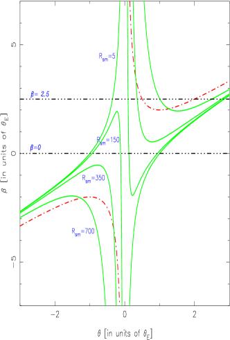
Figure 1: Lensing equation curves for the lens with the scalar charge (solid lines) for four values of $R_{\rm sm}$ and the negative mass lens (dashed-dotted lines). Horizontal dot-dot-dashed lines represent a constant source position. Here $|M|_{\rm lens}=10^{11}\,M_{\odot}$, $z_{\rm source}=3.0$, $z_{\rm lens}=1.3$.

For the case of negative mass objects, the lens will be, most likely, not seen. We would rather expect the existence of compact objects of solar or sub-solar negative mass, as opposed to larger structures whose effects are apparently absent from all deep fields images macro . Then we will not be able to see the images, but only to observe the microlensing light curves, and/or distinctive chromaticity effects (see eiroa ).

Finally, not only gravitational lensing observations can break this degeneracy. Forthcoming supernovae studies, might clearly distinguish between the different FRW models. If we live in a flat or open FRW universe, one of the three cases herein treated disappears. Theoretical investigations in GR and related areas might eventually lead to the proof of the cosmic censorship conjecture, or the energy conditions, and in that case, neither the JNW solution with non-zero scalar charge nor exotic negative mass lenses will be realized. As for the time being, we can not neglect any of these theoretical situations and the best way to attack the problem would be imposing direct astrophysical bounds. The MOA group is currently adapting their alert systems to take into account this kind of exotic lensing P . Maybe great surprises await to be discovered.

A number of dark lens candidates (quasar pairs with no detectable lensing mass) have been reported in the literature, and their true nature is still a matter of an open vigorous debate dark . Current attempts at solving the problem by trying to fit the existing candidates under the lensing by empty dark matter halos do not work rusin02 . Dark lenses are expected to have very small magnification ratios and prominent third images. The majority of current candidates have flux ratio that differ significantly from unity, and do not feature any third image. The absence of quads (four-image systems) makes the current dark lens sample even more peculiar. The type of lenses described here, with their image configurations (always two images, albeit on one side of most probably invisible lens), and magnification ratios (the ratio is much steeper than for the equivalent ordinary lensing, seem to be an interesting possibility for the dark lenses.

The considered cases might be not the only diverging lens systems possible. According to the paper by Amendola et al. waga2 , huge empty voids with radii larger than 100 $h^{-1}$ Mpc can be individually detected via diverging weak lensing. Empty voids with radii 30 $h^{-1}$ Mpc, characteristic of those seen in galaxy redshift surveys, have a lensing signal to noise ratio smaller than unity. Finally, we note that we have considered only strong lensing events, because it is only in this case that the degeneracy is manifested.

- (1) E. L. Turner, J. P. Ostriker, & J. R. Gott III, ApJ, 284 (1984); M. Fukigita et al, ApJ, 393, 3 (1992); R. Gott, M.-G. Park & H.M. Lee, ApJ, 338, 1 (1989).
- (2) L. F. Bloomfield-Torres and I. Waga, Mon. Not. R. Ast. Soc., 279, 712 (1996).
- (3) M. G. Park & J. R. Gott III, ApJ, 489, 476 (1997); M. Franx et al, in The Young Universe. Eds. S. D’Odorico et al. Astronomical Society of the Pacific, 146, ASP Conference Series, p. 142 (1998).
- (4) A. Cooray, A&A, 341, 653 (1999).
- (5) H. Bondi, Rev. Mod. Phys. 29, 423 (1957).
- (6) M. S. Morris and K. S. Thorne, Am. J. Phys. 56, 395 (1987); M. Morris, K. Thorne and U. Yurtserver, Phys. Rev. Lett. 61, 1446 (1988).
- (7) M. Visser, Lorentzian Wormholes (AIP, New York, 1996); L. A. Anchordoqui, S. E. Perez Bergliaffa & D. F. Torres, Phys. Rev. D 55, 5226 (1997); C. Barceló and M. Visser, Phys. Lett. B 466, 127 (1999).
- (8) M. Safonova, G. E. Romero & D. F. Torres, Phys. Rev. D65,023001 (2002).
- (9) M. Safonova, G. E. Romero & D. F. Torres, Mod. Phys. Lett. A16, 153 (2001).
- (10) T. Damour & G. Esposito-Farese, Phys. Rev. Lett, 70, 2220 (1993); A. W. Whinnett Phys. Rev. D61 124014 (2000); A. W. Whinnett & D. F. Torres, Physical Review D60, 104050 (1999).
- (11) F.S. Guzman, T. Matos and H. Villegas, Astron. Nachr, 320, 97 (1999).
- (12) Y.M. Cho and Y.Y. Keum, Class. Quantum Grav., 15, 907 (1998).
- (13) V. Faraoni, Phys. Rev. D62, 023504 (2000).
- (14) D. F. Torres, S. Capozziello, and G. Lambiase, Phys. Rev. D 62, 104012 (2000); D. F. Torres, Nucl. Phys. B626, 377 (2002).
- (15) K.S. Virbharda, D. Narashima, & S.M. Chitre, A&A, 337, 1 (1998).
- (16) K. S. Virbhadra, Int. J. Mod. Phys. D6, 357 (1997).
- (17) Matos T. and Becerril R., Class. Quantum Grav., 18, 2015(2001).
- (18) Dabrowski M. and Schunck F. E., ApJ 535, 316 (2000).
- (19) Janis A.I., Newman E.T. and Winicour J. Phys. Rev. Lett. 20, 878 (1968).
- (20) S. Perlmutter, et al., ApJ, 517, 565 (1999).
- (21) A. Lewis and N. Turok, Phys. Rev. D 65, 043513 (2002).
- (22) R. J. Gott III & M. J. Rees, MNRAS, 1987, 227, 45.
- (23) T. D. Saini , PhD thesis, IUCAA, Pune University, 2001.
- (24) P. Schneider, J. Ehlers, and E. E. Falco, Gravitational Lenses (Springer-Verlag Berlin Heidelberg New York, 1992).
- (25) E. Eiroa, G. E. Romero & D. F. Torres, Mod. Phys. Letters A16, 973 (2001); D. F. Torres, E. Eiroa & G. E. Romero, Mod. Phys. Letters A16, 1849 (2001).
- (26) M. R. S. Hawkings, et al, MNRAS, 291, 811 (1997); D. J. Mortlock, R. L. Webster & P. L. Francis, MNRAS, 309, 836 (1999); C. S. Kochanek, E. E. Falco & Munoz, ApJ, 510, 590(1999); C. Y. Peng et al, ApJ, 524, 572 (1999).
- (27) D. Rusin, astro-ph/0202360.
- (28) P. Yock, private communication (2001).
- (29) L. Amendola, J. A. Frieman, I. Waga, MNRAS 309, 465 (1999)