Post-Newtonian Models of Differentially Rotating Neutron Stars

Abstract

A self-consistent field method is developed, which can be used to construct models of differentially rotating stars to first post-Newtonian order. The rotation law is specified by the specific angular momentum distribution $j(m_{\varpi})$, where $m_{\varpi}$ is the baryonic mass fraction inside the surface of constant specific angular momentum. The method is then used to compute models of the nascent neutron stars resulting from the accretion induced collapse of white dwarfs. The result shows that the ratios of kinetic energy to gravitational binding energy, $\beta$, of the relativistic models are slightly smaller than the corresponding values of the Newtonian models.

I Introduction

In a recent paper liu02 (hereafter Paper II), we demonstrate that the accretion induced collapse (AIC) of a rapidly rotating white dwarf can result in a rapidly rotating neutron star that is dynamically unstable to the bar-mode instability, which is the instability resulting from non-axisymmetric perturbations with angular dependence $e^{\pm 2i\varphi}$. Here $\varphi$ is the azimuthal angle. This instability could emit a substantial amount of gravitational radiation that could be detectable by gravitational wave interferometers, such as LIGO, VIRGO, GEO and TAMA.

However, for this instability to occur, the neutron star must have a $\beta=T/|W|$ greater than a critical value $\beta_{d}\approx 0.25$ (Paper II). Here $T$ is the rotational kinetic energy and $|W|$ is the gravitational binding energy. Only the AIC of white dwarfs that are composed of oxygen, neon and magnesium (O-Ne-Mg white dwarfs) with $\Omega>0.93\Omega_{m}$ can produce neutron stars with such a high value of $\beta$. Here $\Omega$ is the angular velocity of the white dwarf and $\Omega_{m}$ is the angular velocity at which mass shedding occurs on the equatorial surface. This type of source will not be promising for LIGO II because its event rate is not expected to be very high.

Neutron stars are compact objects. General relativistic effects have a significant influence on both the structure and dynamical stability of the stars. Recently, Shibata, Baumgarte, Saijo and Shapiro studied the dynamical stability of differentially rotating polytropes in full general relativity shibata00 and in the post-Newtonian approximation saijo00 . They performed numerical simulations on the differentially rotating polytropes with some specified rotation law. They found that as the star becomes more compact, the critical value $\beta_{d}$ slightly decreases from the Newtonian value $0.26$ to $0.24$ for their chosen rotation law. It is not clear, however, whether their result implies that relativistic effects would destabilize the stars we are studying, for the equilibrium structure of the star will also be changed by relativistic effects. The value of $\beta$ of a relativistic star will not be the same as that of a Newtonian star with the same baryon mass and total angular momentum.

The objective of this paper is twofold. First, we develop a new numerical technique to construct the equilibrium structure of a rotating star with a specified specific angular momentum distribution to first post-Newtonian (1PN) order [i.e., including terms of order $c^{-2}$ higher than the Newtonian terms in the equations of motion]. Then we use this new technique to construct models of neutron stars corresponding to the collapse of the white dwarfs we studied in Paper II and Ref. liu01 (hereafter Paper I) and compare them with the Newtonian models.

Equilibrium models of neutron stars in full general relativity have been built by many authors wilson72 ; bonazzola74 ; butterworth75 ; butterworth76 ; butterworth7679 ; friedman86 ; komatsu89 . The neutron stars studied in the literature are either rigidly rotating or rotating with an ad hoc rotation law. New-born neutron stars resulting from core collapse of massive stars or accretion induced collapse of massive white dwarfs are differentially rotating monchmeyer88 ; janka89 ; fryer01 ; liu01 ; liu02 . It seems plausible that the rotation laws of these neutron stars could be approximated by the specific angular momentum distribution $j(m_{\varpi})$ of the pre-collapse stars (see Paper I and Sec. II.1). Here $m_{\varpi}$ is the baryonic mass fraction inside the surface of constant specific angular momentum. Equilibrium models of Newtonian stars with a specified $j(m_{\varpi})$ have been constructed by many authors ostriker68 ; bodenheimer73 ; pickett96 ; new01 . However, none of these studies, to our knowledge, has been generalized to include the relativistic effects.

If a rotating axisymmetric star is described by a barotropic equation of state, i.e., the total energy density $\epsilon$ is a function of pressure only, then there is a constraint on the rotation law (see Section II.1). This rotational constraint is usually written in the form $u^{0}u_{\varphi}=F(\Omega)$ bardeen70 ; butterworth76 , where $F$ is an arbitrary function. Here $\Omega$ is the angular velocity of the fluid with respect to an inertial observer at infinity; $u^{0}$ is the time component of the four-velocity and $u_{\varphi}=u_{\mu}\varphi^{\mu}$, where $\varphi^{\alpha}$ is the axial Killing vector field of the spacetime. In the Newtonian limit, this constraint reduces to the well-known result that $\Omega$ is constant in the direction parallel to the rotation axis. The major obstacle in the construction of differentially rotating relativistic stars is that it is not clear what function $F$ should be used to produce the desired specific angular momentum distribution $j(m_{\varpi})$. In the next section, we will reformulate the rotational constraint in a way that can be used to impose the rotation law $j(m_{\varpi})$, at least in the 1PN calculations.

The structure of this paper is as follows. In Section II, we give a brief review on the full relativistic treatment of rotating relativistic stars and then reformulate the rotational constraint imposed by the barotropic equation of state. Next, we use the standard 1PN metric and show that the rotational constraint can be solved analytically. We then derive the equations of motion determining the structure of a star to 1PN order. In Section III, we generalize the self-consistent field method of Smith and Centrella smith92 so that it can be used to compute the structure of a star to 1PN order. In Section IV, we apply the numerical method to construct neutron star models resulting from the collapse of the O-Ne-Mg white dwarfs we studied in Paper II and compare them with the corresponding Newtonian models. Finally, we summarize our conclusions in Section V.

II Formalism

In this section, we first give a brief review on the full relativistic treatment of rotating relativistic stars and then reformulate the rotational constraint imposed by the barotropic equation of state (EOS) in Section II.1. Then we derive the equations of motion determining the equilibrium structure of a rotating star to 1PN order in Section II.2. Throughout this chapter, we use the convention that Greek indices run from 0 to 4, 0 being the time component; whereas Latin indices run from 1 to 3 only. A sum over repeated indices is assumed unless stated otherwise. The signature of the metric is $(-+++)$.

II.1 Relativistic hydrodynamics

We want to construct the nascent neutron stars resulting from the AIC of rotating white dwarfs. As in Paper I, we make the following assumptions on the AIC and the collapsed stars.

First, we assume the collapse is axisymmetric. Hence the spacetime, albeit dynamical, has an axial Killing vector field $\varphi^{\alpha}$. Second, we neglect viscosity and assume a perfect fluid stress-energy tensor

$$T^{\mu\nu}=(\epsilon+P)u^{\mu}u^{\nu}+Pg^{\mu\nu}\ ,$$ (1)

where $\epsilon$ is the energy density in the fluid’s rest frame; $P$ is pressure and $u^{\mu}$ is the fluid’s four-velocity, normalized so that $u^{\alpha}u_{\alpha}=-1$. Third, we assume that the collapsed objects can be described by a barotropic EOS, i.e. $\epsilon=\epsilon(P)$. Fourth, we assume there is no meridional circulation in the equilibrium state of the collapsed objects, i.e., the spacetime is nonconvective or circular gourgoulhon93 . In other words, the fluid’s four-velocity can be written as

$$u^{\alpha}=u^{0}\left(t^{\alpha}+\frac{\Omega}{c}\varphi^{\alpha}\right)\ ,$$ (2)

where $t^{\alpha}$ is the timelike Killing vector field of the spacetime of the collapsed star, $c$ is the speed of light, $u^{0}$ is the time component of the four-velocity, and $\Omega$ is the rotational angular velocity measured by an inertial observer at infinity. Finally, we assume that no material is ejected from the star during and after the collapse. Hence the total baryon rest mass $M_{0}$ and the total angular momentum $J$ are conserved.

Let $n$ denote the baryon number density in the fluid’s rest frame. It follows from the baryon number conservation law $\nabla_{\nu}(nu^{\nu})=0$ and conservation of energy-momentum $\nabla_{\nu}T^{\mu\nu}=0$ that (see, e.g., Chapter 22 of Ref. MTW )

$$\frac{d\epsilon}{dn}=\frac{\epsilon+P}{n}\ .$$ (3)

Given a barotropic EOS, the above equation can be integrated, giving

$$n(\epsilon)=n(\epsilon_{0})\,\exp\left[\int_{\epsilon_{0}}^{\epsilon}\frac{d\epsilon^{\prime}}{\epsilon^{\prime}+P(\epsilon^{\prime})}\right]\ .$$ (4)

We define the baryonic rest mass density $\rho=n\bar{m}_{B}$. Here $\bar{m}_{B}$ is the average baryon mass, defined so that

$$\lim_{\epsilon\rightarrow 0}\frac{\epsilon}{\rho c^{2}}=1\ .$$ (5)

It follows bardeen70 from the conservation of baryon number $\nabla_{\nu}(nu^{\nu})=0$, conservation of energy-momentum $\nabla_{\nu}T^{\mu\nu}=0$, and the existence of an axial Killing vector $\varphi^{\alpha}$ that

$$u^{\beta}\nabla_{\beta}j=\frac{dj}{d\tau}=0\ ,$$ (6)

where $\tau$ is the proper time along the fluid particle’s worldline and the specific angular momentum

$$j=\frac{\epsilon+P}{\rho c}u_{\varphi}\ .$$ (7)

Here $u_{\varphi}=u_{\alpha}\varphi^{\alpha}$. In the Newtonian limit, $j=\Omega\varpi^{2}$, which is the Newtonian expression of the specific angular momentum along the rotation axis. Here $\varpi$ is the distance from the rotation axis. Following the arguments in Paper I, we conclude that the final neutron star should have the same baryon mass $M_{0}$, total angular momentum $J$, and specific angular momentum distribution $j(m_{\varpi})$ as the pre-collapse white dwarf.

In the stationary and axisymmetric spacetime of a relativistic star, the Euler equation takes the form bardeen70

$$\frac{\nabla_{\alpha}P}{\epsilon+P}=-u^{\beta}\nabla_{\beta}u_{\alpha}=\nabla_{\alpha}(\ln u^{0})-u^{0}u_{\varphi}\frac{\nabla_{\alpha}\Omega}{c}\ .$$ (8)

Since the EOS is barotropic, the left side of Eq. (8) is a total differential. This imposes a constraint on the rotation law: the integrability condition for Eq. (8) is that the rotation law must have the form $u^{0}u_{\varphi}=F(\Omega)$ bardeen70 ; butterworth76 , where $F$ is an arbitrary function. In the Newtonian limit, this rotational constraint means that $\Omega$ is constant in the direction parallel to the rotation axis. The constraint written in this form is not convenient for our purpose, as our rotation laws are specified by the function $j(m_{\varpi})$. Hence, we formulate the constraint in another way: the integrability condition is that $u^{0}u_{\varphi}\nabla_{\alpha}\Omega$ is an exact differential. In the language of differential forms, we require that $u^{0}u_{\varphi}\tilde{d}\Omega$ be an exact form. This implies that its exterior derivative vanishes:

$$\tilde{d}(u^{0}u_{\varphi}\tilde{d}\Omega)=0\ ,$$ (9)

where $\tilde{d}$ denotes the exterior derivative.

II.2 Post-Newtonian approximation

Following Chandrasekhar chandra65 , we split the energy density into two terms:

$$\epsilon=\rho c^{2}\left(1+\frac{\Pi}{c^{2}}\right)\ .$$ (10)

We adopt the 1PN metric (in Cartesian coordinates) developed by Chandrasekhar, and Blanchet, Damour and Schäfer chandra65 ; blanchet90 ; cutler91 :

$$g_{00} = -\left(1+\frac{2U}{c^{2}}+\frac{2U^{2}}{c^{4}}\right)+O(c^{-6})\ ,$$ (11)

$$g_{0i} = \frac{A_{i}}{c^{3}}+O(c^{-5})\ ,$$ (12)

$$g_{ij} = \left(1-\frac{2U}{c^{2}}\right)\delta_{ij}+O(c^{-4})\ .$$ (13)

The metric components satisfy the gauge condition

$$\sum_{i=1}^{3}\partial_{i}g_{i0}-\frac{1}{2c}\partial_{t}\left(\sum_{i=1}^{3}g_{ii}\right) = O(c^{-5})\ ,$$ (14)

$$\sum_{i=1}^{3}\partial_{i}g_{ij}+\frac{1}{2}\partial_{j}\left(g_{00}-\sum_{i=1}^{3}g_{ii}\right) = O(c^{-4})\ .$$ (15)

In this metric, the components of the four-velocity are

$$u^{0} = 1+\frac{1}{c^{2}}\left(\frac{v^{2}}{2}-U\right)+\frac{1}{2c^{4}}\left(U^{2}-5Uv^{2}+\frac{3}{4}v^{4}+2v^{i}A_{i}\right)+O(c^{-6})\ ,$$ (16)

$$u^{i} = \frac{v^{i}}{c}\left[1+\frac{1}{c^{2}}\left(\frac{v^{2}}{2}-U\right)\right]+O(c^{-5})\ ,$$ (17)

where $v^{i}=cu^{i}/u^{0}$ and $v^{2}=\delta_{ij}v^{i}v^{j}$. The potentials $U$ and $A_{i}$ satisfy the elliptic equations

$$D_{j}D^{j}U+\frac{8\pi G\rho}{c^{2}}U = 4\pi G\rho\left[1+\frac{1}{c^{2}}\left(\Pi+2v^{2}+\frac{3P}{\rho}\right)\right]\ ,$$ (18)

$$D_{j}D^{j}A_{i} = 16\pi G\rho\delta_{ik}v^{k}\ ,$$ (19)

where $D_{j}$ denotes the covariant derivative compatible with the three dimensional flat-space metric, and $G$ is the gravitational constant. We introduce cylindrical coordinates $(\varpi,\varphi,z)$ with $\partial/\partial\varphi$ being the axial Killing vector, and $\varpi=\sqrt{x^{2}+y^{2}}$. In this coordinate system, the velocity vector potential $A_{i}$ has only one component: $A_{\varphi}=xA_{y}-yA_{x}$. Let $Q=A_{\varphi}/\varpi$. Then $Q$ satisfies the equation

$$D^{j}D_{j}Q-\frac{Q}{\varpi^{2}}=16\pi G\rho\Omega\varpi\ .$$ (20)

To 1PN order, we have

$$cu^{0}u_{\varphi}=\varpi^{2}\Omega\left(1+\frac{K}{c^{2}}\right)\ ,$$ (21)

where

$$K=v^{2}-4U+\frac{Q}{v}\ .$$ (22)

Since $u^{0}u_{\varphi}\nabla_{\alpha}\Omega$ is an exact differential, we can write

$$\nabla_{\alpha}f=\varpi^{2}\Omega\left(1+\frac{K}{c^{2}}\right)\nabla_{\alpha}\Omega\ ,$$ (23)

where $f$ is a scalar function. The rotational constraint (9) gives only one nontrivial equation for $\Omega$ in a stationary and axisymmetric spacetime. To 1PN order, Eq. (9) can be solved analytically, giving

$$\Omega(\varpi,z)=\Omega_{0}(\varpi)+\frac{\varpi\partial_{\varpi}\Omega_{0}}{2c^{2}}[K(\varpi,z)-K_{0}(\varpi)]\ ,$$ (24)

where $\Omega_{0}(\varpi)\equiv\Omega(\varpi,0)$ and $K_{0}(\varpi)\equiv K(\varpi,0)$. Eq. (23) can then be integrated and we obtain, up to an arbitrary additive constant,

$$f(\varpi,z) = \frac{\varpi^{2}}{2}\Omega_{0}^{2}(\varpi)-\int_{0}^{\varpi}d\varpi^{\prime}\,\varpi^{\prime}\Omega_{0}^{2}(\varpi^{\prime})$$ (26)

$$+\frac{1}{c^{2}}\left[\varpi^{2}\Omega_{0}(\varpi)\,\Omega_{1}(\varpi,z)+\frac{\varpi^{2}}{2}\Omega_{0}^{2}(\varpi)K_{0}(\varpi)-I_{1}(\varpi)\right]\ ,\ \ \ \ \ \ \ \$$

where

$$\Omega_{1}(\varpi,z) = \frac{\varpi\partial_{\varpi}\Omega_{0}}{2}[K(\varpi,z)-K_{0}(\varpi)]\ ,$$ (27)

$$I_{1}(\varpi) = \int_{0}^{\varpi}d\varpi^{\prime}\,\Omega_{0}^{2}(\varpi^{\prime})\left[\varpi^{\prime}K_{0}(\varpi^{\prime})+\frac{\varpi^{\prime 2}}{2}\partial_{\varpi}K_{0}(\varpi^{\prime})\right]\ .$$ (28)

It is convenient to define an auxiliary function

$$h=c^{2}\int_{0}^{P}\frac{dP^{\prime}}{\epsilon(P^{\prime})+P^{\prime}}\ .$$ (29)

This quantity is defined only inside the star. The boundary of the star is given by the surface $h=0$. In the Newtonian limit, $h$ reduces to the specific enthalpy. The Euler equation (8), to 1PN order, can be written in integral form:

$$h(\varpi,z) = \int_{0}^{\varpi}d\varpi^{\prime}\,\varpi^{\prime}\Omega_{0}^{2}(\varpi^{\prime})-U+C$$ (31)

$$+\frac{1}{c^{2}}\left(\frac{\varpi^{4}}{4}\Omega_{0}^{4}-2\varpi^{2}\Omega_{0}^{2}U+Qv-\frac{\varpi^{2}\Omega_{0}^{2}K_{0}}{2}+I_{1}\right)\ ,\ \ \ \ \$$

where $C$ is a constant and all quantities outside the integral are evaluated at $(\varpi,z)$.

The structure of the star is determined once a rotation law is given. The rotation law is specified by the specific angular momentum distribution function $j(m_{\varpi})$, which is determined by the pre-collapse white dwarf (see Paper I). Straightforward calculations using Eqs. (7), (10), (11), (12), (13), (16), (17), (24) and (27) give

$$j=\varpi^{2}\Omega_{0}\left[1+\frac{1}{c^{2}}\left(\frac{v^{2}}{2}-3U+\Pi+\frac{P}{\rho}+\frac{\Omega_{1}}{\Omega_{0}}+\frac{Q}{v}\right)\right]\ .$$ (32)

To compute $m_{\varpi}$, the baryonic mass fraction inside the surface of constant $j$, we first need to determine the surfaces on which $j$ is constant. In the Newtonian case, the surfaces of constant $j$ are cylinders. This is not true in general in the relativistic case (at least not in the coordinate system we are using). Let $[\varpi+\eta(\varpi,z)/c^{2},z]$ denote the surface of constant $j$ that intersects the equatorial plane at cylindrical coordinate radius $\varpi$. Hence we have

$$j[\varpi+\eta(\varpi,z)/c^{2},z] = j(\varpi,0)\ ,$$ (33)

$$\eta(\varpi,0)=0\ .$$ (34)

Expanding the left side of Eq. (33) to $O(c^{-2})$, we obtain

$$\eta(\varpi,z)=-c^{2}\frac{j(\varpi,z)-j_{0}(\varpi)}{\partial_{\varpi}j_{0}(\varpi)}\ ,$$ (35)

where $j_{0}(\varpi)\equiv j(\varpi,0)$. Using Eq. (32), we obtain

$$\eta=-\frac{\varpi\Omega_{0}\pounds(\Pi-3U+P/\rho)+\varpi\Omega_{1}+\pounds(Q)}{2\Omega_{0}+\varpi\partial_{\varpi}\Omega_{0}}\ ,$$ (36)

where $\pounds(q)\equiv q(\varpi,z)-q(\varpi,0)$. The baryon mass $M_{\varpi}$ inside the volume $V_{\varpi}$ bounded by the surface of constant $j$ is given by

$$M_{\varpi} = \int_{V_{\varpi}}\rho u^{\mu}n_{\mu}\,dV$$ (37)

$$= 2\pi\int_{-\infty}^{\infty}dz^{\prime}\,\left[\varpi\rho^{*}(\varpi,z^{\prime})\frac{\eta(\varpi,z^{\prime})}{c^{2}}+\int_{0}^{\varpi}d\varpi^{\prime}\,\varpi^{\prime}\rho^{*}(\varpi^{\prime},z^{\prime})\right]\ ,\ \ \ \ \ \$$ (38)

where $n^{\mu}$ is the unit vector orthogonal to the surface of constant $t$; $dV$ is the proper volume element in the constant $t$ hypersurface, and

$$\rho^{*}=\rho\left[1+\frac{1}{c^{2}}\left(\frac{v^{2}}{2}-3U\right)\right]\ .$$ (39)

The baryonic mass fraction is then given by

$$m_{\varpi}=\frac{M_{\varpi}}{M_{0}}\ ,$$ (40)

where $M_{0}$ is simply the value of $M_{\varpi}$ at $\varpi=R_{e}$, the equatorial radius of the star. It is convenient to define the normalized specific angular momentum

$$j_{n}=\frac{M_{0}}{J}j\ .$$ (41)

Straightforward calculations from Eq. (32) give

$$\Omega_{0}^{2}=\frac{\lambda^{2}j_{n}^{2}}{\varpi^{4}}-\frac{1}{c^{2}}\left[\Omega_{0}^{2}\left(\varpi^{2}\Omega_{0}^{2}-6U_{0}+2\Pi_{0}+\frac{2P_{0}}{\rho_{0}}\right)+\frac{2\Omega_{0}Q_{0}}{\varpi}\right]\ ,$$ (42)

where $\lambda=J/M_{0}$ and the subscript “0” in the above equation means that the quantity is evaluated at $(\varpi,0)$. The integrated Euler equation (31) becomes

$$h=\lambda^{2}\psi-U+C+\frac{1}{c^{2}}\left(\frac{v^{4}}{4}-2Uv^{2}+Qv-\frac{1}{2}v^{2}K_{0}+I_{2}\right)\ .$$ (43)

Here

$$\psi(\varpi) = \int_{0}^{\varpi}\frac{j_{n}^{2}(m_{\varpi^{\prime}})}{\varpi^{\prime 3}}\,d\varpi^{\prime}\ ,$$ (44)

$$I_{2}(\varpi) = \int_{0}^{\varpi}d\varpi^{\prime}\,\left[\frac{1}{2}v_{0}^{2}\partial_{\varpi}K_{0}+2\varpi^{\prime}\Omega_{0}^{2}\left(U_{0}-\Pi_{0}-\frac{P_{0}}{\rho_{0}}\right)-Q_{0}\Omega_{0}\right]\ ,\ \ \ \ \ \ \$$ (45)

where all the quantities in the integrands are evaluated at $\varpi=\varpi^{\prime}$.

The rotational kinetic energy $T$ and gravitation potential energy $W$ of a relativistic star are given by (see, e.g., komatsu89 )

$$T = \frac{1}{2}\int\Omega\,dJ=\frac{1}{2c}\int\Omega T_{\mu\nu}n^{\mu}\varphi^{\nu}\,dV\ ,$$ (46)

$$W = -[(M_{p}-M)c^{2}+T]\ ,$$ (47)

where the proper mass $M_{p}$ and gravitational mass $M$ are

$$M_{p} = \frac{1}{c^{2}}\int\epsilon u^{\mu}n_{\mu}\,dV$$ (48)

$$M = -\frac{2}{c^{2}}\int\left(T_{\alpha\beta}-\frac{1}{2}T^{\sigma}_{\sigma}g_{\alpha\beta}\right)t^{\alpha}n^{\beta}\,dV\ .$$ (49)

Both $T$ and $W$ are independent of gauge in a spacetime that is stationary, axisymmetric and nonconvective. The expressions for $T$ and $W$ to 1PN order are

$$T = \int\frac{1}{2}\rho v^{2}\left[1+\frac{1}{c^{2}}\left(v^{2}-6U+\Pi+\frac{P}{\rho}+\frac{Q}{v}\right)\right]\,d^{3}x\ ,$$ (50)

$$W = \int(\rho v^{2}+\rho U+3P)\,d^{3}x-\frac{1}{c^{2}}\int\rho\left(\frac{5}{2}U^{2}+\frac{11}{2}Uv^{2}-\frac{9}{8}v^{4}\right.$$ (52)

$$\left.-\frac{Qv}{2}-\Pi v^{2}-\Pi U-\frac{3Pv^{2}}{2\rho}+\frac{6PU}{\rho}\right)\,d^{3}x\ ,$$

where $d^{3}x\equiv\varpi\,d\varpi\,dz\,d\varphi$.

Given the total baryon mass $M_{0}$, total angular momentum $J$, normalized specific angular momentum distribution $j_{n}(m_{\varpi})$, and EOS, we have to solve Eqs. (18), (20), (43), (32), and (40) consistently to determine the structure of the differentially rotating star. We shall discuss how these equations can be solved numerically in the next section.

III Numerical method

In this section, we develop a self-consistent field technique to calculate the structure of a relativistic star with the rotation law specified by the normalized specific angular momentum distribution $j_{n}(m_{\varpi})$. Our method is a generalization of the one used by Smith and Centrella smith92 , which is a modified version of Hachisu’s self-consistent field method hachisu86 .

The self-consistent field method is an iteration procedure. Suppose in a certain iteration step, we have $h(\varpi,z)$ and $\Omega_{0}(\varpi)$ in a cylindrical grid, we first evaluate the quantities $\rho$, $P$ and $\Pi$ from the EOS. Then we compute the potentials $U$ and $Q$ by solving the elliptic equations (18) and (20). Since the velocity potential $Q$ always appears in the 1PN terms of the equations of motion, we can replace $\Omega$ on the right side of Eq. (20) by $\Omega_{0}$. The angular velocity $\Omega$, as well as $v=\varpi\Omega$, outside the equatorial plane are determined by Eqs. (22) and (24). Next, we compute the baryonic mass fraction $m_{\varpi}$ using Eqs. (36), (38), (39) and (40). The function $\psi$ is then calculated by Eq. (44). During each iteration, we fix two parameters, which we choose to be the central energy density $\epsilon_{c}$ [or equivalently, $h_{c}=h(0,0)$] and the equatorial radius $R_{e}$. The constants $C$ and $\lambda^{2}$ in Eq. (43) are then given by

$$C = h_{c}+U_{c}\ ,$$ (53)

$$\lambda^{2} = \frac{1}{\psi}\left[U-C-\frac{1}{c^{2}}\left(\frac{v^{4}}{4}-2v^{2}U+Qv-\frac{v^{2}K_{0}}{2}+I_{2}\right)\right]\ ,$$ (54)

where $U_{c}=U(0,0)$ and all the quantities in the second equation are evaluated at the equatorial surface of the star. Finally, we update $h$ by Eq. (43) and update $\Omega_{0}$ by solving the algebraic equation (42). We repeat the procedure until $h$ and $\Omega_{0}$ converge to the desired accuracy.

When the star becomes flattened, the iteration scheme described above does not converge. This is fixed by generalizing the modified scheme suggested in Ref. pickett96 : the variables $h$ and $\Omega_{0}$ in the $(i+1)$-th iteration, $h_{i+1}$ and $(\Omega_{0})_{i+1}$ are changed to

$$h_{i+1} = h_{i}\delta+h^{\prime}(1-\delta)\ ,$$ (55)

$$(\Omega_{0})_{i+1} = (\Omega_{0})_{i}\delta+\Omega^{\prime}_{0}(1-\delta)\ ,$$ (56)

where $h^{\prime}$ and $\Omega^{\prime}_{0}$ are the quantities determined by Eqs. (43) and (42). The parameter $\delta$ ($0\leq\delta<1$) is used to control the changes of $h$ and $\Omega_{0}$ in an iteration step. For a very flattened configuration, we need to use $\delta>0.9$ to ensure convergence, and it takes more than 100 iterations for the models to converge to a fractional accuracy of $10^{-5}$. In the standard self-consistent field method, one only needs to solve for the density distribution $\rho$ (or equivalently, the enthalpy distribution $h$) self-consistently. In our self-consistent field method, we also need to solve for the equatorial angular velocity distribution $\Omega_{0}$ self-consistently. This is the main difference between the standard scheme and our proposed scheme, apart from the fact that the equations of motion in the 1PN case are more complicated.

The self-consistent field method described above computes stars with a given central energy density $\epsilon_{c}$ and equatorial radius $R_{e}$. However, we want to construct a star with a given total baryon mass $M_{0}$ and total angular momentum $J$. To do this, we first compute a model of non-rotating spherical star by solving the 1PN structure equations for nonrotating stars in isotropic coordinates. We use the density distribution as an initial guess to construct a model with slightly different $\epsilon_{c}$ and $R_{e}$. We then build models with different values of $\epsilon_{c}$ and $R_{e}$ until we end up with the model having the desired baryon mass and angular momentum.

For a rapidly rotating configuration, the equatorial radius extends to $R_{e}>1000~{}\rm{km}$ and the polar radius is approximately $R_{p}\approx 10~{}\rm{km}$ in our coordinate system. Hence we use a nonuniform cylindrical grid to perform most of the computations. The resolution near the center of the star is about $0.4~{}\rm{km}$, whereas the resolution is about $6.5~{}\rm{km}$ near the equatorial surface of the star. We double the resolution to check the convergence. For a given $\epsilon_{c}$ and $R_{e}$, the fractional differences of the baryon mass $M_{0}$ and angular momentum $J$ between the two resolution grids are less than $10^{-5}$ even for the rapidly rotating cases.

We adopt the Bethe-Johnson EOS bethe74 for densities above $10^{14}~{}\rm{g}~{}\rm{cm}^{-3}$, and BBP EOS baym71 for densities in the range $10^{11}-10^{14}~{}\rm{g}~{}\rm{cm}^{-3}$. The EOS for densities below $10^{11}~{}\rm{g}~{}\rm{cm}^{-3}$ is joined by that of the pre-collapse white dwarfs, which is the EOS of a zero-temperature ideal degenerate electron gas with electrostatic corrections derived by Salpeter salpeter61 . We are mainly interested in the structure of the most rapidly rotating neutron stars. The central densities of these stars are around $4\times 10^{14}~{}\rm{g}~{}\rm{cm^{-3}}$ (see the next section), and ideas about the EOS in this relatively low density region have not changed very much since 1970’s.

The baryon masses of the neutron stars we compute in this chapter are around $1.4M_{\odot}$. For a non-rotating spherical star of this baryon mass, $c^{2}R/GM\approx 6$ for the EOS we adopt. Here $M\approx 1.3M_{\odot}$ is the gravitational mass and $R\approx 12~{}\rm{km}$ is the circumferential radius of the star. Hence we expect that the second and higher order post-Newtonian terms will give about $1/6^{2}\approx$3% corrections to our models.

The effect of higher post-Newtonian terms can also be estimated by the virial identity to 1PN order (see the Appendix). We define a dimensionless quantity

$$\zeta=\frac{Z}{W_{N}}\ ,$$ (57)

where

$$Z = \int[\sigma v^{2}+3P-\sigma(\varpi\partial_{\varpi}U+z\partial_{z}U)]\,d^{3}x$$ (60)

$$+\frac{1}{c^{2}}\int[6PU+\rho\Omega_{0}\varpi Q+(2P-\sigma v^{2}-4\rho U)(\varpi\partial_{\varpi}U+z\partial_{z}U)$$

$$+\rho\varpi\Omega_{0}(\varpi\partial_{\varpi}Q+z\partial_{z}Q)]\,d^{3}x\ ,$$

$$W_{N} = -\int\sigma(\varpi\partial_{\varpi}U+z\partial_{z}U)\,d^{3}x\ ,$$ (61)

$$\sigma = \rho\left[1+\frac{1}{c^{2}}\left(v^{2}-2U+\Pi+\frac{P}{\rho}\right)\right]\ .$$ (62)

The dimensionless quantity $\zeta$ is a measure of the fractional error of our equilibrium models due to higher post-Newtonian corrections (see the Appendix).

IV Results

We only construct neutron star models corresponding to the collapse of O-Ne-Mg white dwarfs (i.e., the Sequence III white dwarfs in Paper II), because these neutron stars are the most likely to undergo a dynamical instability and emit strong gravitational waves.

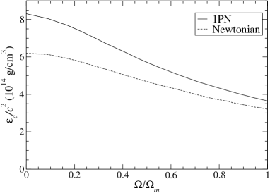
Figure 1: The central densities $\epsilon_{c}/c^{2}$ of differentially rotating neutron stars as a function of $\Omega/\Omega_{m}$ of the pre-collapse white dwarfs. Both Newtonian and 1PN results are shown for stars having the same $M_{0}$ and $J$.

Figure 1 shows the central densities $\epsilon_{c}/c^{2}$ of the resulting neutron stars as a function of $\Omega/\Omega_{m}$, where $\Omega$ is the angular frequency of the pre-collapse white dwarf, and $\Omega_{m}$ is the angular frequency of the maximally rotating white dwarf in the sequence. Both Newtonian and 1PN results are shown for stars having the same $M_{0}$ and $J$. We see that the central energy densities for the 1PN models are higher than the Newtonian models. This is expected because relativistic effects tend to make the stars more compact. The difference in $\epsilon_{c}$ decreases as the star becomes more rapidly rotating.

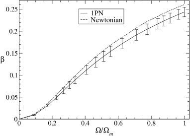
Figure 2: The value of $\beta$ of the resulting neutron stars as a function of $\Omega/\Omega_{m}$ of the pre-collapse white dwarfs. The vertical bars through the 1PN curve show $\beta\pm\delta\beta$ of selected equilibrium models, where $\delta\beta$ is the error of $\beta$ due to higher post-Newtonian corrections estimated by Eq. (64).

Figure 2 shows the value of $\beta=T/|W|$ of the neutron stars as a function of $\Omega/\Omega_{m}$ for both the Newtonian and 1PN models. To estimate the possible error of $\beta$ due to higher post-Newtonian effects, we use the formula

$$\delta\beta = \beta\left|\frac{\delta T}{T}-\frac{\delta W}{W}\right|$$ (63)

$$\leq \beta\left(\left|\frac{\delta T}{T}\right|+\left|\frac{\delta W}{W}\right|\right)\ .$$ (64)

We found that the quantity $U^{2}/c^{4}$ is the largest second post-Newtonian terms we neglected in the whole calculation. Hence we estimate that

$$\left|\frac{\delta T}{T}\right| \approx \frac{1}{T}\int T_{i}\frac{U^{2}}{c^{4}}\,d^{3}x\ ,$$ (65)

$$\left|\frac{\delta W}{W}\right| \approx \left|\frac{1}{W}\int W_{i}\frac{U^{2}}{c^{4}}\,d^{3}x\right|\ ,$$ (66)

where $T_{i}$ and $W_{i}$ are the integrands in Eqs. (50) and (52), respectively. The vertical bars in Fig. 2 show $\beta\pm\delta\beta$ of selected equilibrium models [using Eqs. (64)–(66) for $\delta\beta$]. The result suggests that relativistic effect lowers the value of $\beta$ for stars of given $M_{0}$ and $J$. The maximum $\beta$ of these neutron stars is 0.24, which is 8% lower than the Newtonian case (0.26). However, the error bars also suggest that higher post-Newtonian corrections could change the values of $\beta$ significantly.

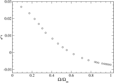
Figure 3: The virial quantity $\zeta$ defined in Eq. (57) for the equilibrium neutron star models, parametrized by $\Omega/\Omega_{m}$ of the pre-collapse white dwarfs.

Figure 3 shows the virial quantity $\zeta$ for our equilibrium neutron star models. This quantity is a measure of the fractional correction to the equilibrium structure of the stars due to higher post-Newtonian effects. We see that $\zeta$ is smaller than 0.03 for all the models we computed, which is in accord with our estimate near the end of Sec. III.

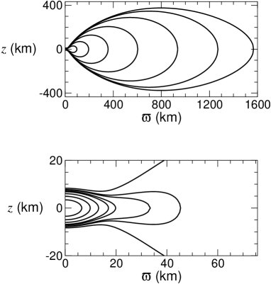
Figure 4: Meridional density contours of the neutron star resulting from the AIC of a rigidly rotating O-Ne-Mg white dwarf with $\Omega/\Omega_{m}=0.964$. This neutron star has $\beta=0.238$. The contours in the upper graph denote, from inward to outward, $\epsilon/\epsilon_{c}=10^{-4}$, $10^{-5}$, $10^{-6}$, $10^{-7}$, $10^{-8}$, $10^{-9}$ and 0. The contours in the lower graph denote, from inward to outward, $\epsilon/\epsilon_{c}$= 0.8, 0.6, 0.4, 0.2, 0.1, $10^{-2}$, $10^{-3}$ and $10^{-4}$. The central density of the star is $\epsilon_{c}/c^{2}=3.8\times 10^{14}~{}\rm{g}~{}\rm{cm}^{-3}$.

The structure of the neutron stars is not much different from the Newtonian models. Stars with $\beta\gtrsim 0.1$ all contain a high-density central core of size about 20 km, surrounded by a low-density torus-like envelope. The size of the envelope ranges from 100 km (for stars with $\beta\sim 0.1$) to over 500 km (for $\beta\gtrsim 0.2$). Figure 4 shows the density contour of a typical rapidly rotating neutron star. This figure looks basically the same as Fig. 3 of Paper II, which shows the density contours of the same star computed with Newtonian gravity. The $\beta$ of this star is 0.238, which is somewhat smaller than the Newtonian value 0.255.

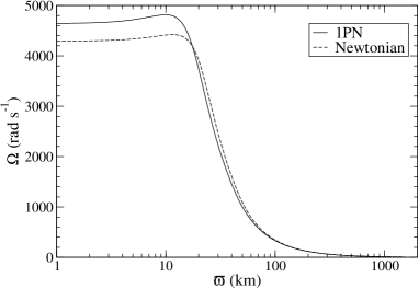
Figure 5: The equatorial angular velocity $\Omega_{0}(\varpi)$ of the neutron star in Fig. 4.

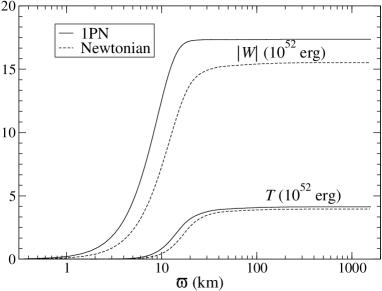
Figure 6: The distribution of the rotational kinetic energy $T$ and gravitational binding energy $|W|$ of the material inside the radius $\varpi$, for the neutron star in Fig. 4.

Figure 5 shows the equatorial angular velocity distribution $\Omega_{0}(\varpi)$ of the same star. We see that the angular velocity in the inner core of the star ($\varpi\lesssim 20~{}\rm{km}$) in the 1PN model is slightly larger than that of the corresponding Newtonian model. This is expected because relativistic effects make the star more compact. The material is compressed more in the 1PN model, and should rotate faster due to the conservation of angular momentum. Figure 6 shows the distribution of rotational kinetic energy $T$ and gravitational binding energy $|W|$ of the material contained within cylindrical radius $\varpi$. The two quantities approach their asymptotic values at $\varpi\approx 30~{}\rm{km}$. This is due to the high central condensation of the star. Both $T$ and $|W|$ in the 1PN model are larger than the corresponding Newtonian model. The kinetic energy $T$ is larger because the star rotates faster. However, the difference between the two $T$-curves decreases as we move away from the rotation axis. This is because most of the kinetic energy of the star is from the region $10~{}\rm{km}\lesssim\varpi\lesssim 30~{}\rm{km}$, in which relativistic effects are less important. On the other hand, the gravitational binding energy is mainly contributed from the material in the inner region $\varpi\lesssim 20~{}\rm{km}$, in which relativistic effects are important. As a result, the $T/|W|$ value of the relativistic model is somewhat less than in the corresponding Newtonian model.

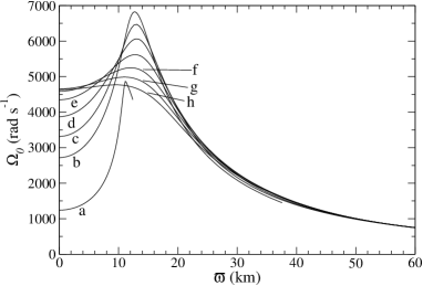
Figure 7: The equatorial rotational angular velocity $\Omega_{0}$ as a function of $\varpi$ for $\varpi<60~{}\rm{km}$. These neutron stars result from the AIC of the pre-collapse white dwarfs with $\Omega/\Omega_{m}$ equal to (a) 0.090, (b) 0.23, (c) 0.30, (d) 0.41, (e) 0.55, (f) 0.71, (g) 0.86 and (h) 1.00.

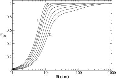
Figure 8: The cylindrical mass fraction $m_{\varpi}$ as a function of $\varpi$ for the neutron star models in Fig. 7. The curves and the corresponding models are identified by the degrees of central condensation: the higher the degree of central condensation, the lower the value of $\Omega/\Omega_{m}$.

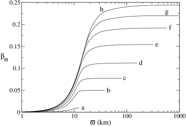
Figure 9: The value of $\beta_{\varpi}$ as a function of $\varpi$ for the neutron star models in Fig. 7.

Figure 7 shows the equatorial angular velocity $\Omega_{0}$ for several selected models in the central region near the rotation axis. The shape of the curves are very similar to those of the Newtonian models (see Fig. 4 of Paper II). However, the angular velocities in the 1PN models are all slightly larger than the Newtonian models in the inner core.

Figure 8 shows the baryonic mass fraction $m_{\varpi}$ verses $\varpi$ for the selected models in Fig. 7. As in the Newtonian case (see Fig. 5 of Paper II), the mass is highly concentrated in the inner core of the star. The degree of central condensation decreases as the star rotates faster. However, more than 80% of the mass is contained within a 30 km radius even for the most rapidly rotating star, where the outer envelope extends to over 1000 km. The collapsed object can be regarded as a neutron star of size about 20 km surrounded by an accretion torus.

Figure 9 shows $\beta_{\varpi}$, the $T/|W|$ of the material inside the surface of constant $\varpi$, for the selected models in Fig. 7. The shape of the curves are qualitatively the same as those in the Newtonian models ( see Fig. 6 of Paper II), although the values of $\beta_{\varpi}$ are slightly smaller. All the curves level off at $\varpi\approx 30-50~{}\rm{km}$, suggesting that the material in the outer layers does not have much influence on the overall dynamical stability of the star.

V Conclusions

We have generalized the self-consistent field method so that it can be used to compute models of differentially rotating stars to 1PN order with a specified angular momentum distribution $j(m_{\varpi})$. We also applied this new method to construct models of nascent neutron stars resulting from the collapse of massive O-Ne-Mg white dwarfs we studied in Paper II and compare them with the corresponding Newtonian models.

We found that the 1PN models are more compact and rotate faster. Our calculations also suggest that the 1PN models have smaller values of $\beta$ than the corresponding Newtonian models. The highest value of $\beta$ these neutron stars can achieve is 0.24, which is 8% smaller than the Newtonian case. Higher post-Newtonian corrections may change the values of $\beta$, but our estimate suggests that they will still be smaller than those of the Newtonian models. We estimate that the fractional error of our 1PN models due to our neglecting higher order post-Newtonian terms is about 3%.

The fact that relativistic effects lower the values of $\beta$ can be understood by the following heuristic argument. Relativistic effects make a star more compact. Hence the gravitational binding enetgy $|W|$ increases. The compactness of the star also make it rotate faster due to conservation of angular momentum. Hence the rotational kinetic energy $T$ also increases. However, most of the kinetic energy comes from material slightly away from the center of the star (in the region $10~{}{\rm km}\lesssim\varpi\lesssim 30~{}{\rm km}$ for the star in Fig. 6), where relativistic effects are less important compared to the region near the center. On the other hand, the gravitational binding energy $|W|$ is contributed mainly from material near the center of the star (in the region $\varpi\lesssim 20~{}{\rm km}$ for the star in Fig. 6). As a result, the increase in $T$ is not as much as the increase in $|W|$, and so the value of $\beta$ decreases.

We have demonstrated that relativistic effects could lower the value of $\beta$ of a star with a given baryon mass $M_{0}$ and angular momentum $J$. Shibata, Baumgarte, Shapiro and Saijo shibata00 ; saijo00 demonstrated that relativistic effects also lower the critical value $\beta_{d}$ for the dynamical instability by a similar amount. It will be interesting to find out which of these two effects is more important. Careful numerical 1PN stability analyses must be carried out to determine whether or not relativistic effects destabilize the stars.

*

Appendix A Virial theorem to 1PN order

Virial theorems in full general relativity were formulated by Bonazzola and Gourgoulhon bonazzola73 ; gourgoulhon94 ; bonazzola94 , and have been proved to be useful as a consistency check for numerical computation of rotating star models (see, e.g., bonazzola74 ; bonazzola93 ; cook96 ). These virial identities are not very convenient to implement since they involve integrals over the entire two or three-dimensional volume, but our computational domain only extends to the region slightly outside the surface of the star. Chandrasekhar derived a virial identify to the 1PN order chandra65 in which integrations are only performed over the interior of a star. However, it involves a double volume integral. In this appendix, we shall derive another virial identify which is correct to the 1PN order and is easier to compute than the Chandrasekhar identity. This expression is useful to estimate the error of our equilibrium neutron star models due to higher post-Newtonian effects.

We start with Eq. (67) of Ref. chandra65 , which is the Euler equation to 1PN order note :

$$\partial_{i}(\sigma v_{j}v^{i})+\left(1+\frac{2U}{c^{2}}\right)\partial_{j}P+\sigma\left(1+\frac{v^{2}}{c^{2}}\right)\partial_{j}U-\frac{4}{c^{2}}\rho v_{j}v^{i}\partial_{i}U$$ (67)

$$+\frac{1}{c^{2}}\rho v^{i}(\partial_{i}A_{j}-\partial_{j}A_{i})+\frac{4\rho U}{c^{2}}\partial_{j}U=0 \ ,$$ (68)

$$\sigma=\rho\left[1+\frac{1}{c^{2}}\left(v^{2}-2U+\Pi+\frac{P}{\rho}\right)\right] \ .$$ (69)

Here we have set all partial time derivatives to zero. The equation is valid to 1PN order for the metric (11)–(13). Multiplying Eq. (68) by $x^{j}$, summing over $j$ and integrating over $d^{3}x\equiv dx\,dy\,dz=\varpi\,d\varpi\,dz\,d\varphi$, we obtain, after integration by parts,

$$\int\{\sigma v^{2}+3P-\sigma x^{j}\partial_{j}U+\frac{1}{c^{2}}[2P(3U+x^{j}\partial_{j}U)-\sigma v^{2}x^{j}\partial_{j}U+4\rho x^{j}v_{j}v^{i}\partial_{i}U$$ (70)

$$-\rho v^{i}x^{j}(\partial_{i}A_{j}-\partial_{j}A_{i})-4\rho Ux^{j}\partial_{j}U]\}\,d^{3}x=0 \ .$$ (71)

In a stationary, axisymmetric and circular spacetime, $x^{j}v_{j}=x^{j}A_{j}=0$. In cylindrical coordinates, we have

$$x^{j}\partial_{j}U = \varpi\partial_{\varpi}U+z\partial_{z}U\ ,$$ (72)

$$v^{i}x^{j}(\partial_{j}A_{i}-\partial_{i}A_{j}) = \varpi\Omega(\varpi\partial_{\varpi}Q+z\partial_{z}Q)+\varpi\Omega Q\ ,$$ (73)

where $Q=(xA_{y}-yA_{x})/\varpi$. Hence Eq. (71) becomes, to 1PN order,

$$\int\{\sigma v^{2}+3P-\sigma(\varpi\partial_{\varpi}U+z\partial_{z}U)+\frac{1}{c^{2}}[6PU+\rho\Omega_{0}\varpi Q\hskip 142.26378pt$$ (74)

$$+(2P-\sigma v^{2}-4\rho U)(\varpi\partial_{\varpi}U+z\partial_{z}U)+\rho\varpi\Omega_{0}(\varpi\partial_{\varpi}Q+z\partial_{z}Q)]\}\,d^{3}x=0\ .\hskip 28.45274pt$$ (75)

Equation (75) is our virial identity. It involves a volume integral over the interior of the star. In the Newtonian limit, it reduces to the familiar form $2T+3\Lambda+W=0$, where $\Lambda=\int P\,d^{3}x$.

Let $Z$ be the left side of Eq. (75) and define a dimensionless quantity

$$\zeta = Z/W_{N}\ \ \ ,$$ (76)

$$W_{N} = -\int\sigma(\varpi\partial_{\varpi}U+z\partial_{z}U)\,d^{3}x\ .$$ (77)

In the Newtonian limit, $\zeta=(2T+3\Lambda+W)/W$, which is a quantity often used as a measure of the fractional numerical error of Newtonian equilibrium models caused by finite grid size.

Our equilibrium models are constructed by solving Eq. (43), which agrees with Eq. (68) to 1PN order. Hence the quantity $\zeta$ measures the fractional error of our models due to second and higher post-Newtonian corrections, and also the numerical error due to finite grid size.

References

- (1) Y.T. Liu, Phys. Rev. D., 65, 124003 (2002) (Paper II).
- (2) Y.T. Liu and L. Lindblom, Mon. Not. R. Astro. Soc., 324, 1063 (2001) (Paper I).
- (3) M. Shibata, T.W. Baumgarte and S.L. Shapiro, Astrophys. J., 542, 453 (2000).
- (4) M. Saijo, M. Shibata, T.W. Baumgarte and S.L. Shapiro, Astrophys. J., 548, 919 (2001).
- (5) J.R. Wilson, Astrophys. J., 176, 195 (1972).
- (6) S. Bonazzola and J. Schneider, Astrophys. J., 191, 273 (1974).
- (7) E.M. Butterworth and J.R. Ipser, Astrophys. J. Lett., 200, 103 (1975);
- (8) E.M. Butterworth and J.R. Ipser, Astrophys. J., 204, 200 (1976).
- (9) E.M. Butterworth, Astrophys. J., 204, 561 (1976); E.M. Butterworth, Astrophys. J., 231, 219 (1979).
- (10) J.L. Friedman, J.R. Ipser and L. Parker, Astrophys. J., 304, 115 (1986).
- (11) H. Komatsu, Y. Eriguchi and I. Hachisu, Mon. Not. R. Astro. Soc., 237, 355 (1989); H. Komatsu, Y. Eriguchi and I. Hachisu, Mon. Not. R. Astro. Soc., 239, 153 (1989).
- (12) R. Mönchmeyer and E. Müller, in NATO ASI on Timing Neutron Stars, ed. Ögelman H., D. Reidel Publ. Comp., Dordrecht 1988.
- (13) H.-T. Janka, R. Mönchmeyer, Astro. & Astrophys., 209, L5 (1989); H.-T. Janka, R. Mönchmeyer, Astro. & Astrophys., 226, 69 (1989).
- (14) C.L. Fryer, D.E. Holz and S.A. Hughes, Astrophys. J., 565, 430 (2002).
- (15) J.P. Ostriker and J. W-K. Mark, Astrophys. J., 151, 1075 (1968); J.P. Ostriker and P. Bodeneimer, Astrophys. J., 151, 1089 (1968).
- (16) P. Bodeneimer and J.P. Ostriker, Astrophys. J., 180, 159 (1973).
- (17) B.K. Pickett, R.H. Durisen and G.A. Davis, Astrophys. J., 458, 714 (1996).
- (18) K.C.B. New and S.L. Shapiro, Astrophys. J., 548, 439 (2001).
- (19) J.M. Bardeen, Astrophys. J., 162, 71 (1970).
- (20) S. Chandrasekhar, Astrophys. J., 142, 1488 (1965).
- (21) L. Blanchet, T. Damour and G. Schaäfer, Mon. Not. R. Astro. Soc., 242, 289 (1990).
- (22) C. Cutler, Astrophys. J., 374, 248 (1991).
- (23) C. W. Misner, K.S. Thorne and J.A. Wheeler, Gravitation (Freeman and Company 1973).
- (24) S. Smith, J.M. Centrella, in Approaches to Numerical Relativity, ed. R.d’Inverno. (Cambridge Univ. Press, New York 1992).
- (25) I. Hachisu, Astrophys. J. Supp., 61, 479 (1986).
- (26) H.A. Bethe and M.B. Johnson, Nucl. Phys. A, 230, 1 (1974).
- (27) G. Baym, H.A. Bethe and C.J. Pethick, Nucl. Phys. A, 175, 225 (1971).
- (28) E.E. Salpeter, Astrophys. J., 134, 669 (1961).
- (29) S. Bonazzola, Astrophys. J., 182, 335 (1973).
- (30) E. Gourgoulhon and S. Bonazzola, Phys. Rev. D., 48, 2635 (1993).
- (31) E. Gourgoulhon and S. Bonazzola, Class. Quantum Grav., 11, 443 (1994).
- (32) S. Bonazzola and E. Gourgoulhon, Class. Quantum Grav., 11, 1775 (1994).
- (33) S. Bonazzola, E. Gourgoulhon, M. Salgado and J.A. Marck, Astron. Astrophys., 278, 421 (1993).
- (34) G.B. Cook, S.L. Shapiro and S.A. Teukolsky, Phys. Rev. D., 53, 5533 (1996).
- (35) The relationships between our variables and those used in Ref. chandra65 are: and , where the variables appeared in Ref. chandra65 are denoted by the superscript ∗.