Black-hole threshold solutions in stiff fluid collapse

Abstract

Numerical studies of the gravitational collapse of a stiff ($P=\rho$) fluid have found the now familiar critical phenomena, namely scaling of the black hole mass with a critical exponent and continuous self-similarity at the threshold of black hole formation. Using the equivalence of an irrotational stiff fluid to a massless scalar field, we construct the critical solution as a scalar field solution by making a self-similarity ansatz. We find evidence that this solution has exactly one growing perturbation mode; both the mode and the critical exponent, $\gamma\simeq 0.94$, derived from its eigenvalue agree with those measured in perfect fluid collapse simulations. We explain why this solution is seen as a critical solution in stiff fluid collapse but not in scalar field collapse, and conversely why the scalar field critical solution is not seen in stiff fluid collapse, even though the two systems are locally equivalent.

I Introduction

Solutions of Einstein’s equations that lie at the threshold of black-hole formation have provided a unique insight into gravitational dynamics during the past decade. The advent of sophisticated numerical techniques and powerful computers has facilitated the study of this regime.

Critical phenomena were first discovered in the gravitational collapse of a real, massless scalar field, in the evolution of generic 1-parameter families of asymptotically flat initial data [1]. During the time evolution, the matter either disperses (subcritical data) or collapses to form a black hole (supercritical data). The critical solution exists precisely at the threshold of black hole formation. This solution has several interesting properties which also are at least approximately shared by near-critical solutions. First, the masses of black holes formed in supercritical evolutions obey a universal scaling law,

$$M_{\mathrm{BH}}\propto|p-p^{\star}|^{\gamma},$$ (1)

where $p$ is the parameter of a given 1-parameter family of data, and $p^{\star}$ is its critical value such that black holes are formed for $p>p^{\star}$. Thus, in this model, infinitesimally small black holes can be formed by adjusting $p$ to be sufficiently close to $p^{\star}$. Second, near-critical evolutions go through a universal intermediate phase that exhibits self-similar echoing near the origin. The echoes are periodic in logarithmic time, so that the critical solution (universal intermediate attractor) is, in fact, discretely self-similar. Empirically, it is found that the critical exponent, $\gamma\simeq 0.374$, is the same for all 1-parameter families of massless scalar field initial data.

As they have now been found in a wide variety of general relativistic self gravitating systems, critical phenomena are considered to be generic features of “tuned” gravitational collapse. Interested readers are directed to [2] for a comprehensive review. In brief, the threshold of black hole formation singles out well-defined critical solutions which typically have additional symmetry (beyond that which might have been imposed via the formulation of the model under consideration), and which, though unstable by construction, tend to have precisely one unstable mode in perturbation theory. The critical solutions are typically unique (up to a dynamically irrelevant overall rescaling): the unstable mode is consequently also unique, as is the growth factor associated with the mode. The growth factor can then be immediately related, via ideas familiar from renormalization group studies, to a scaling exponent defined, for example, via (1) [3, 4].

The critical solutions which have been observed so far have either a time-translational or a scale-translational symmetry [5, 6]; these two types have also been dubbed Type I and Type II, respectively. Within each of the two symmetry categories, solutions can be further differentiated according to whether the extra symmetry appears continuously or discretely. Thus, Type I solutions are static or periodic, and display a mass gap at threshold. As one tunes closer and closer to criticality, the static/periodic intermediate attractor (star-like solution) persists for a lifetime $\tau\sim\sigma\ln|p-p^{\star}|$ where $\sigma$ is the reciprocal Lyapunov exponent associated with the unstable mode. Type II solutions, on the other hand, are either continuously or discretely self-similar (CSS or DSS), exhibit infinitesimal mass at threshold, and generically have naked singularities at the origin in the precisely critical limit. In the supercritical case, the black hole mass scales according to the relation (1), where again, the scaling exponent $\gamma$ is the reciprocal Lyapunov exponent of the critical solution’s single unstable mode. The remainder of this paper concerns only Type II behavior, and the key distinction between the two solutions which will be discussed is that one is CSS while the other is DSS. We also note that a key feature of the Type II solutions which have been computed thus far via direct tuning of PDE solutions is that, virtually by definition of existing at the threshold of black hole formation, they do not contain apparent horizons.

One of the models in which critical phenomena have been studied most extensively is that of spherically symmetric collapse of perfect fluids with the one-parameter scale-free equation of state (EOS)

$$P=k\rho.$$ (2)

Here $P$ is the fluid’s isotropic pressure, $\rho$ the energy density, and $0<k\leq 1$ is a constant (the single parameter of the EOS). Critical collapse in this context was first considered by Evans and Coleman for the specific case $k=1/3$ (radiation equation of state) [3]. These authors not only found a continuously self-similar (CSS) critical solution via evolution of families of initial data, but also constructed that same critical solution more directly by adopting a CSS ansatz, and then solving the resulting boundary-value eigenproblem. This work was quickly followed by examination of the stability properties of this and related CSS fluid solutions within the context of perturbation theory [4, 7, 8]. Working from the CSS ansatz, these studies identified single-mode-unstable CSS solutions for $0\leq k\lesssim 0.89$, indicating that the black hole threshold solutions were CSS (and thus Type II) for $k$ in this range. The absence of solutions for $k\gtrsim 0.89$ was intriguing, and hinted that the critical solutions for such cases might have different properties—in particular, there were suspicions that one or both of the assumptions of 1) regularity at the origin, and 2) continuous self-similarity might break down at $k\sim 0.89$. However, CSS critical solutions with regular origins for $0.89\lesssim k\leq 1$ were subsequently found, through fluid evolutions [9, 10], as well as via adoption of the CSS ansatz [9], with, from the point of view of the PDE evolutions, no obviously special changes in solution properties at $k\sim 0.89$ [9].

The existence of a CSS critical solution in the limiting case of the stiff fluid ($k=1$) was particularly surprising to many, as the spherically symmetric stiff fluid is formally equivalent to a spherically symmetric real scalar field. [The technicalities of this equivalence are detailed below in Section II A for the stiff fluid, and in Appendix A for an arbitrary barotropic equation of state $P=P(\rho)$.] Thus, one might have naively expected that the critical solution appearing in one system would automatically arise as the critical solution in the other. However, the DSS solution of scalar field collapse and the CSS solution of stiff fluid collapse are distinctly different solutions.

Two fairly obvious questions then arise: 1) Why is the CSS critical solution found in stiff fluid collapse not observed in massless scalar critical field collapse? 2) Why is the DSS scalar field critical solution not seen in stiff fluid collapse? The answer to the second question is relatively trivial, and has been well known in the critical-collapse community for some time—the DSS scalar field critical solution corresponds to a perfect fluid with negative (as well as positive) pressures and densities, and hence cannot arise in fluid collapse scenarios where energies and densities, are, by fiat, constrained to be positive. As discussed in more detail below, the resolution of the second question is somewhat more subtle, but in essence amounts to the observation that the CSS critical solution, when interpreted in the scalar field context, contains an apparent horizon and therefore cannot and does not sit at the black hole threshold. This appears closely related to the phenomena observed in Lechner et al’s study of general relativistic non-linear sigma models [5], where the absence of CSS solutions at black hole threshold above a certain strength in coupling parameter is correlated with the fact that the CSS solutions at those coupling values have apparent horizons.

II A continuously self-similar (CSS) scalar field solution with one growing mode

In this section we construct the critical solution for spherically symmetric stiff fluid collapse using the equivalence between the scalar field and the stiff fluid to work in the scalar field variables. We first describe this equivalence between the two matter models, give the field equations in Bondi coordinates, then restrict them to a continuously self-similar ansatz. We then study the spacetime structure and perturbation modes for two solutions, one of which is the desired critical solution.

A The correspondence between the stiff fluid and the scalar field

A stiff fluid is a perfect fluid with equation of state, $P=\rho$. The stress-energy tensor for the stiff fluid can therefore be written as

$$T^{ab}=\rho(2u^{a}u^{b}+g^{ab})\;.$$ (3)

Here $\rho$ is the total energy density of the fluid as measured by an observer moving with a fluid element, and hence having a normalized 4-velocity $u^{a}$. If the 4-velocity is irrotational ($\nabla_{[a}u_{b]}=0$), we can write $u^{a}$ in terms of the gradient of a scalar field. (In spherical symmetry the fluid is automatically irrotational.) We introduce a scalar field $\psi$ with future-pointing timelike gradient such that

$$\nabla_{a}\psi=\sqrt{2\rho}\,u_{a},$$ (4)

where $\nabla_{a}$ is the metric-compatible covariant derivative. This defines $\psi$ up to an additive constant, whose value is irrelevant. The inverse relation between the fluid and the scalar field is then given by

$$\rho = -{\textstyle\frac{1}{2}}\nabla_{c}\psi\nabla^{c}\psi,$$ (5)

$$u_{a} = {\nabla_{a}\psi\over\sqrt{-\nabla_{c}\psi\nabla^{c}\psi}}.$$ (6)

Expressing the stress-energy tensor (3) in terms of $\psi$ gives

$$T^{ab}=\nabla^{a}\psi\nabla^{b}\psi-{\textstyle\frac{1}{2}}(\nabla_{c}\psi\nabla^{c}\psi)g^{ab}.$$ (7)

The conservation of energy-momentum, $\nabla_{a}T^{ab}=0$, implies that $\psi$ satisfies the massless, minimally coupled scalar wave equation

$$\nabla_{c}\nabla^{c}\psi=0.$$ (8)

This establishes a local, one-to-one relationship between irrotational (in particular, spherically symmetric) stiff fluid solutions and massless scalar field solutions with timelike gradient. The existence of massless scalar field solutions that also have spacelike and null gradients is relevant later when we discuss the relation between interpolating families of stiff fluid solutions and those of scalar field collapse. A more general treatment, applicable for equations of state of the form $P=P(\rho)$, is given in Appendix A.

Although the perfect fluid and scalar field models are related by this mathematical equivalence, differences remain in their physical interpretation. Generally, a fluid is a phenomenological model derived via thermodynamic considerations of a large number of particles interacting through elastic collisions. The fluid density, $\rho$, and four-velocity, $u^{a}$, are continuum variables defined in terms of the fundamental discrete variables in a limiting procedure. The fluid energy density, for example, is defined in terms of the total energy in an arbitrary volume, in the limit that the volume element becomes infinitesimally small. Thus, a fluid is a continuum model of a discrete system containing a thermodynamically significant number of particles; the model is expected to fail as the large-particle-number limit is violated, $\rho\to 0$. Indeed, the fluid equations become singular in this limit.

Given the thermodynamic motivation for perfect fluid models, one conventionally imposes physical constraints on the fluid’s energy density and four-velocity, namely that $\rho>0$, and that $u^{a}$ is timelike. The fluid equations may admit solutions in violation of these constraints, in which case the solution may be discarded, or matched with other solutions to create a physical spacetime. One could argue against accepting these physical constraints, but one would then be adopting a view of a fluid seemingly at odds with the usual assumption of an underlying discrete system.

The scalar field, on the other hand, is fundamentally a continuum model, and does not directly represent the behavior of a discrete system of particles. Consequently, its solutions are generally not subject to the constraints discussed in the previous paragraph. Thus, the assumptions made in constructing the perfect fluid model allow only a restricted class of scalar field solutions—those with $\nabla^{a}\psi\nabla_{a}\psi<0$—to be interpreted as physical fluid solutions.

B Coordinate system and field equations

The general spherically symmetric line element can be written in Bondi coordinates as

$$ds^{2}=-g\overline{g}du^{2}-2gdudr+r^{2}(d\theta^{2}+\sin^{2}\theta d\phi^{2})\;,$$ (9)

where $g=g(u,r)$ and $\overline{g}=\overline{g}(u,r)$. The coordinate $r$ has geometrical meaning in terms of the proper area of $r=$ const. 2-spheres. We demand that the critical solution be regular at the origin; elementary flatness at $r=0$ then dictates that $g(u,0)=\overline{g}(u,0)$. The relation between the fluid density and scalar field in these coordinates is

$$\rho=\frac{\partial_{r}\psi}{2g}(2\partial_{u}\psi-\overline{g}\partial_{r}\psi)\;.$$ (10)

A local mass function $m(u,r)$ is defined by

$$1-\frac{2m(u,r)}{r}\equiv g^{ab}\nabla_{a}r\nabla_{b}r=\frac{\overline{g}}{g}\;,$$ (11)

where $r$ is understood to be a function on spacetime.

Looking ahead to the application of the CSS ansatz, it is convenient to express the Einstein equations using variables adapted to a scale symmetry:

$$x=-r/u\;,\qquad\qquad\qquad\tau=-\ln(-u)\;.$$ (12)

This coordinate change is applied directly to the Einstein equations (not to the line element), which then become

$$x\overline{g}^{\prime} = g-\overline{g}\;,$$ (13)

$$x(\ln g)^{\prime} = 4\pi j^{2}\;,$$ (14)

$$(\overline{g}/g)\dot{\ }+x(\overline{g}/g)^{\prime} = {8\pi(j+\dot{\psi})}\left[(x-\overline{g})j+x\dot{\psi}\right]/g\;.$$ (15)

Here a prime (^′) represents differentiation with respect to $x$, a dot ($\dot{\ }$) means differentiation with respect to $\tau$, and we have also introduced an auxiliary field, $j(u,r)$, defined by

$$x\,\psi^{\prime}=j\;.$$ (16)

Finally, the scalar wave equation of motion (8) becomes

$$(\psi+j)\dot{\ }+(x-{\overline{g}}/{2})j^{\prime}=\frac{j}{2x}(g-2x)\;.$$ (17)

Now that the Einstein equations have been written in terms of the new variables, the CSS ansatz will reduce them to a system of ODEs.

C Continuously self-similar solutions

Self-similar solutions representing scalar field collapse have been studied by Brady [11] and Christodoulou [12]. We present here only those details that are essential to our discussion; the interested reader can consult the above-cited references for further details.

The existence of a homothetic symmetry (continuous scale symmetry) in a spherical spacetime implies that the metric coefficients $g$ and $\overline{g}$ depend only on $x=-r/u$, and that the scalar field is of the form

$$\psi=\overline{h}(x)+\kappa\tau\;,$$ (18)

where $\overline{h}$ is a function to be determined, and $\kappa$ is a positive constant. Restricting equations (13)–(17) to the self-similar ansatz gives

$$x\,\overline{g}^{\prime} = g-\overline{g}\;,$$ (19)

$$x(\ln g)^{\prime} = 4\pi j^{2}\;,$$ (20)

$$g-\overline{g} = 4\pi[2\kappa^{2}x-(\overline{g}-2x)(j^{2}+2\kappa j)]\;,$$ (21)

$$x\overline{h}^{\prime} = j\;,$$ (22)

$$x(2x-{\overline{g}})j^{\prime} = -2\kappa x+{j}(g-2x)\;.$$ (23)

These equations are singular when $\overline{g}=2x$. This corresponds to a similarity horizon in spacetime, that is a null hypersurface of constant $x$ coordinate. With a slight abuse of terminology, it is also a sonic surface of the corresponding stiff fluid. We rescale the coordinate $u$ by a constant factor such that $x=1$ when $\overline{g}=2x$. Note that this means that the usual convention $g=\overline{g}=1$ at the origin $x=0$ does not hold.

In order to be regular in the past, say at $u=-1$, the threshold solution must be analytic at the origin and at the similarity horizon $x=1$. This is impossible for general values of $\kappa$, but we expect to find analytic solutions for isolated values of $\kappa$ [3].

Christodoulou [12] has derived a closed form solution, satisfying these conditions, when $4\pi\kappa^{2}=1/3$. This is a Friedmann-Robertson-Walker cosmological solution, and is not the similarity solution observed in numerical simulations of gravitational collapse. We use it here only to test our numerical methods on an exact solution. Using a two point shooting method to search for analytic solutions at other values of $\kappa$, we find a second solution when $4\pi\kappa^{2}\simeq 0.577$. This solution does correspond to the stiff fluid critical solution, as discussed below in Section II E, but first we discuss its properties as a massless scalar field solution.

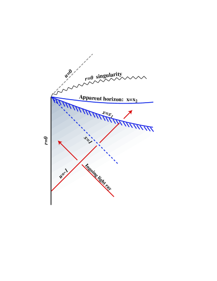
FIG. 1.: A spacetime diagram showing the self-similar scalar field solution with $4\pi\kappa^{2}\simeq 0.577$. The apparent horizon, the similarity horizon at $x=1$, and the surface on which the energy density $\rho$ vanishes are all shown. The shaded region, where the scalar field gradient is timelike, can be identified with a physical stiff fluid solution.

The spacetime structure of the $4\pi\kappa^{2}\simeq 0.577$ solution is sketched in Fig. 1. There is a strong curvature singularity at $r=0$ and $u=0$; this is a point, in the sense that it can be surrounded by an arbitrarily small sphere in spacetime. The center of spherical symmetry, $x=0$, for $u<0$ is made regular by our ansatz, and so is the past light cone of the singularity, $x=1$. The scalar field gradient is timelike for $0\leq x<x_{1}$, with $x_{1}\simeq 1.07$. In that region, the scalar field matter can also be interpreted as a stiff fluid. The surface $x=x_{1}$ is a regular spacelike surface to the future of $x=1$, on which the scalar field gradient is null. In the fluid interpretation this corresponds to the limit in which the fluid 4-velocity becomes null, and the comoving fluid energy density goes to zero. For $x>x_{1}$, the scalar field gradient is spacelike, and the scalar field cannot be interpreted as a stiff fluid given the usual physical constraints on the scalar field’s gradient. The spacelike surface $x=x_{2}\simeq 1.2$ to the future of $x=x_{1}$, is an apparent horizon, i.e., outgoing null rays have zero expansion on this hypersurface. Since $x=x_{2}$ is also a singular point of the differential equations (13)–(17), there is some concern that the hypersurface may be geometrically singular too. Nevertheless, since $r$ is finite along $x=x_{2}$ (except at $u=0$) and $\overline{g}/g=1-2m/r=0$, we conclude that the mass function and all curvature invariants are finite here, as are the scalar field and its derivatives (in a regular coordinate system). Thus, the apparent horizon is non-singular, and the region to its future is trapped. We have not continued the solution to larger values of $x$, but from the singularity theorems we know that to the future of the apparent horizon there is a central $r=0$ strong curvature singularity. This solution belongs in Class II(a) described in Table I of Ref. [11].

D Stability analysis

Having constructed this CSS scalar field solution, we now turn to an examination of its stability properties. As mentioned in the introduction, we expect a critical solution to have a single unstable mode, an insight that results from efforts to understand the black hole mass scaling near the critical point [4, 7, 13]. We therefore expand each of the fields about its self-similar background value:

$$g = g_{0}(x)+g_{1}(x,\tau)\;,$$ (24)

$$\overline{g} = \overline{g}_{0}(x)+\overline{g}_{1}(x,\tau)\;,$$ (25)

$$j = j_{0}(x)+j_{1}(x,\tau)\;,$$ (26)

$$\psi = \overline{h}_{0}(x)+\kappa\tau+\overline{h}_{1}(x,\tau)\;.$$ (27)

The subscript $0$ indicates a regular solution of Eqs. (13)–(17); the subscript $1$ is used to indicate linear perturbations about this solution. In terms of these fields, the perturbation equations become:

$$x\,\overline{h}_{1}^{\prime} = j_{1}\;,$$ (28)

$$x\,\overline{g}_{1}^{\prime} = g_{1}-\overline{g}_{1}\;,$$ (29)

$$x\,g_{1}^{\prime} = 4\pi\left[g_{1}j_{0}^{2}+2g_{0}j_{0}j_{1}\right]\;,$$ (30)

$$2x(j_{1}+\overline{h}_{1})\dot{\ } = x(\overline{g}_{0}-2x)j_{1}^{\prime}+j_{1}(g_{0}-2x)$$ (32)

$$\mbox{\ \ \ \ }+j_{0}g_{1}+\overline{g}_{1}xj_{0}^{\prime}\;.$$

To satisfy elementary flatness at the origin, we set $g_{1}(0,\tau)=\overline{g}_{1}(0,\tau)=0$ and $j_{1}(0,\tau)=0$.

We have used two independent numerical methods to search for the growing modes of Eqs. (28)–(32), a shooting method and a matrix eigenvalue method. Each method has particular strengths. Shooting allows accurate determination of the unstable modes but relies on an initial guess close to the ultimate answer. For this reason, it is difficult to confirm that all the relevant modes have been found without further analysis. The matrix eigenvalue method appears to be less accurate than shooting, but it provides a scheme to determine all the modes at one time and thus confirm that we have identified all growing modes. The observed agreement between the two methods confirms that there is one unstable mode and two gauge modes. We describe each method in turn; Table I summarizes our numerical results.

TABLE I.: Numerical results for the modes of the continuously self similar scalar field solution discussed in the text. Listed in columns 3 through 7 are the mode eigenvalues, $\lambda$, and, where relevant, corresponding scaling exponents, $\gamma\equiv 1/\lambda$, computed using the two methods described in text. Also listed is the scaling exponent $\gamma_{\rm PDE}$ estimated from solution of the full equations of motion [9]. Quoted uncertainties are estimates based on the maximum discontinuity at the fitting point for the shooting method and convergence tests for the matrix method.

Mode	$\lambda_{\rm exact}$	$\lambda_{\rm shoot}$	$\gamma_{\rm shoot}$	$\lambda_{\rm matrix}$	$\gamma_{\rm matrix}$	$\gamma_{\rm PDE}$
physical unstable	$---$	$1.0654\pm 0.0005$	$0.9386\pm 0.0005$	$1.055\pm 0.01$	$0.95\pm 0.01$	$\lesssim 0.96$
gauge shift	$1$	$1.0000\pm 0.0005$	$---$	$1.013\pm 0.01$	$---$	—
gauge rescale	$0$	$0.0000\pm 0.0005$	$---$	$0.000\pm 0.00$	$---$	—

1 Shooting method

This method provides direct computation of the eigenmodes of the perturbation equations (28)–(32) by recasting them as an eigenvalue problem. Consider solutions which separate in the form $f_{1}(x,\tau)=e^{\lambda\tau}\widehat{f}_{1}(x;\lambda)$, where $\lambda$ is a complex number, and the fields $\widehat{f}_{1}(x;\lambda)$ are also complex. Equations (28)–(32) then reduce to a set of ordinary differential equations

$$x\,\widehat{\overline{h}}_{1}^{\prime} = \widehat{j}_{1}\;,$$ (33)

$$x\,\widehat{\overline{g}}_{1}^{\prime} = \widehat{g}_{1}-\widehat{\overline{g}}_{1}\;,$$ (34)

$$x\,\widehat{g}_{1}^{\prime} = 4\pi\left[\widehat{g}_{1}j_{0}^{2}+2g_{0}j_{0}\widehat{j}_{1}\right]\;,$$ (35)

$$2x\lambda(\widehat{j}_{1}+\widehat{\overline{h}}_{1}) = x(\overline{g}_{0}-2x)\widehat{j}_{1}^{\prime}+\widehat{j}_{1}(g_{0}-2x)$$ (37)

$$\mbox{\ \ \ \ }+j_{0}\widehat{g}_{1}+\widehat{\overline{g}}_{1}xj_{0}^{\prime}\;.$$

Growing modes have real, positive $\lambda$ demonstrating the existence of an instability. As explained above, analyticity of the solutions at the origin ($x=0$) and the similarity horizon ($x=1$) is required since the critical solution observed in numerical simulations must be smooth everywhere. Analyticity determines the power series solution about $x=0$ up to three real parameters corresponding to $\tan^{-1}[(\mathrm{Im}\,\widehat{j}_{1})/(\mathrm{Re}\,\widehat{j}_{1})]|_{x=0}$, $\mathrm{Re}\lambda$ and $\mathrm{Im}\lambda$. The amplitude $|\widehat{j}_{1}(0)|$ sets the scale of the perturbations and may be set to unity without loss of generality. Similarly, the power series solution about $x=1$ is determined up to two complex (four real) parameters–$\widehat{j}_{1}(1)$ and $\widehat{\overline{h}}_{1}(1)$. Equations (33)–(37) were solved using a 4th order adaptive Runge-Kutta scheme, shooting from $x=0$ and $x=1$ to a fitting point at $x=0.5$ until the seven parameters were adjusted to produce a smooth solution everywhere on the interval.

There is one physical unstable mode with $\lambda\simeq 1.065$ when $4\pi\kappa^{2}=0.577$. This suggests that the critical exponent is $\gamma=1/\lambda\simeq 0.939$, which is consistent with the numerical results for stiff fluid collapse where $\gamma\lesssim 0.96$ [9]. In addition to the unstable mode, there are modes with $\lambda\simeq 1.000$ and $\lambda\simeq 0.000$. These modes correspond to the symmetries $u\to u+{\rm const.}$ and $\psi\to\psi+{\rm const.}$ of the background CSS solutions respectively, and do not change the physical spacetime. Thus, these are “gauge modes”, and finding them at the right place is a (weak) test of our numerical methods.

For completeness, we also searched for unstable modes of the CSS solution with $4\pi\kappa^{2}=1/3$, but found only the two gauge modes as expected.

2 Matrix eigenvalue method

As the CSS solution presented above is not the threshold solution in massless scalar field critical phenomena, it is important to ensure that we have not missed any other unstable modes. One method to do this is to write the perturbation equations as $u_{,\tau}=Lu$ and to look directly for eigenvalues $\lambda$ of the time evolution operator $L$.

For this, we have used the background and perturbation equations in polar-radial coordinates (they are given for example in [14]), but this is accidental: we could equally well have implemented the time evolution operator method in Bondi coordinates, or the shooting method in polar-radial coordinates.

The equations for the linear matter perturbation can formally be written as the system

$$u_{,\tau}=A(x)u_{,x}+B(x)u+C(x)w,$$ (38)

where $u(x,\tau)$ stands for the two first-order matter perturbation variables and $w(x,\tau)$ stands for the two metric perturbations. (This is true both for Bondi coordinates and polar-radial coordinates.) The metric perturbations are not evolved, but are reconstructed from the matter perturbations by ODEs of the form

$$w_{,x}=D(x)w+E(x)u.$$ (39)

The matrices $A$, $B$, $C$, $D$ and $E$ depend on the background solution.

The perturbation equations were discretized in space but not in time. The resulting set of equations can formally be written as $d\hat{u}_{N}/d\tau=L_{N}\hat{u}_{N}$. Here $\hat{u}_{N}$ is the approximation of $u$ on a grid with $N$ points in the range $0\leq x\leq 1$, and the matrix $L_{N}$ is the corresponding finite difference approximation of the time evolution operator. The results quoted below were obtained at a resolution of $N=800$, making $L_{N}$ a $1600^{2}$ matrix. The eigenvectors and eigenvalues of this matrix were then computed to machine precision using a standard linear algebra package. Most of the eigenvectors of $L_{N}$ depend on the finite differencing scheme, but those with the highest values of ${\rm Re}\lambda$ converge to modes of the continuum equations with increasing $N$, and the corresponding eigenvalues converge to the continuum eigenvalues $\lambda$.

The matrix eigenvalue method, in polar-radial coordinates, finds the growing mode at $\lambda\simeq 1.055$, and the gauge modes at $\lambda\simeq 1.013$ and $\lambda=0$. This last value is exact to machine precision as the $\psi\to\psi+{\rm const.}$ gauge mode decouples in these coordinates. Using the second-order convergence of our finite difference scheme, we estimate the uncertainty in these results to be $0.01$ for our finest grid of $N=800$ points. This estimate is consistent with the error in $\lambda$ for the gauge mode, which should be $\lambda=1$, as well as with the independent results from the shooting method in Bondi coordinates.

With $L_{N}$ already obtained, it was straightforward to implement the Lyapunov analysis described by Koike, Hara and Adachi [8], and compare it with our matrix eigenvalue method. We just had to combine $L_{N}$ with a fourth-order Runge-Kutta discretization in $\tau$ in order to obtain a finite difference version of the evolution equations. (Such a method is variously called a method of lines, or a semi-discrete method.) We then used the Lyapunov method to obtain the highest few eigenvalues. In the limit in which the timestep $\Delta\tau$ is chosen much smaller than the spatial resolution $\Delta x$, the resulting values of $\lambda$ coincide with those of the direct eigenvector method to machine precision, as one would expect. However, our method has the crucial advantage of producing all the top eigenvectors (modes) as well as the eigenvalues, whereas the Lyapunov method produces only the one eigenvector associated with the highest eigenvalue. Finding subdominant eigenvectors is important here because there are two gauge modes in the system of equations whose eigenvalues may be higher than that of the unstable physical mode.

E Comparison with the observed stiff fluid critical solution

Having constructed a CSS scalar field solution with a single unstable mode, we now compare it with the stiff fluid critical solution. To facilitate the comparison, we adopt the polar-radial coordinates, $(t,r)$, and variables (fluid and metric) used in the fluid studies [8, 9]. This is effected by introducing $t=-r\xi(x)$ where

$$x(\ln\xi)^{\prime}=\frac{\overline{g}}{\overline{g}-x}\;,$$ (40)

and $\xi(1)=1$. The metric and fluid variables are

$$a^{2} = g/\overline{g}\;,$$ (41)

$$\omega = 4\pi r^{2}a^{2}\rho=2\pi[2x(j^{2}+\kappa)/\overline{g}-j^{2}]\;,$$ (42)

$$v^{2} = \frac{[j(\overline{g}-x)-x\kappa]^{2}}{x^{2}(j+\kappa)^{2}}\;.$$ (43)

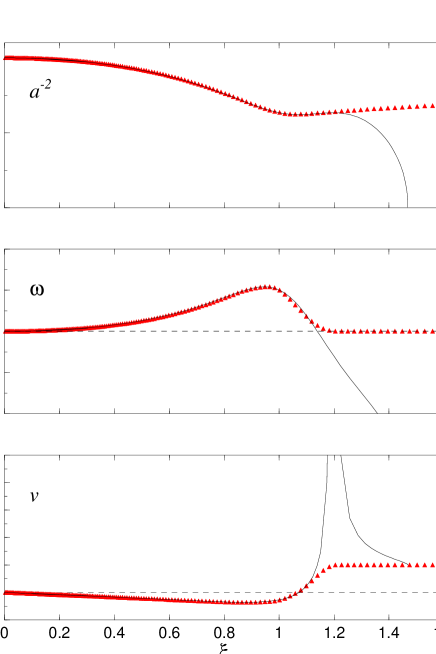
FIG. 2.: The CSS solution with $4\pi\kappa^{2}\simeq 0.577$ (solid lines), obtained by solving the ODEs in Eqs. (19)–(23) and Eq. (40), compared to a near critical solution computed using the PDE code in Ref.[9] (dotted lines). The similarity horizon is at $\xi=1$. There is excellent agreement between the two solutions up to, and sightly beyond, the similarity horizon. The self-similar scalar field solution cannot be identified with a stiff fluid solution beyond $\xi\simeq 1.14$ where the gradient of the field is spacelike.

Fig. 2 shows our CSS scalar field solution and the stiff perfect fluid critical solution computed by evolving tuned initial data, as described in Ref. [17, 9]. There is excellent agreement between the scalar field solution and the fluid solution inside the similarity horizon ($\xi=1$), and slightly beyond. The two solutions differ when $\xi\gtrsim\xi_{1}\simeq 1.14$, however. Here the energy density, $\rho$, of a fluid equivalent to the scalar field vanishes and the fluid 3-velocity reaches unity. In the numerical evolutions of the perfect fluid, a floor is imposed to maintain $\rho\geq 0$ and a timelike 4-velocity in the simulations. This accounts for the dramatic difference between the solutions at larger values of $\xi$, and is discussed in detail in Section III B.

In addition to this direct comparison of the perfect fluid and scalar field solutions, we verify that the solutions share the same stability properties. As mentioned previously, the unstable mode of the CSS scalar field solution gives a critical scaling exponent of $\gamma\simeq 0.94$, which agrees with the perfect fluid estimate of $\gamma\lesssim 0.96$. Finally, we can directly compare the unstable modes as shown in Fig. 3.

FIG. 3.: This figure shows the unstable mode for the metric function $a$, comparing the mode of the CSS scalar field solution (solid line) with that of the perfect fluid (triangles). The modes match particularly well when $\xi\lesssim\xi_{1}$ ($\xi_{1}\simeq 1.14$), where the two solutions are equivalent. Beyond this point, where the fluid and scalar field are no longer equivalent, the modes diverge as expected. The perfect fluid mode was calculated using from two near-critical fluid simulations. As the mode has no intrinsic magnitude, the fluid data were scaled to match the scalar field mode.

III The role of the scalar field CSS solution in gravitational collapse

There are at least three regular self-similar, spherically symmetric scalar field solutions: the cosmological CSS solution found by Christodoulou, the CSS solution with one growing mode found in stiff fluid collapse [9] and studied here, and the DSS critical solution with one growing mode [1] examined in more detail in Ref. [13]. Turning to the questions raised in the Introduction, we examine why the stiff fluid and scalar field critical solutions are not identical, given the (local) equivalence between the two matter models.

A Self-similar solutions in massless scalar field collapse

The cosmological solution ($4\pi\kappa^{2}=1/3$) has additional symmetries; it is actually a spatially flat Friedmann solution driven by an homogeneous scalar field. It has no growing perturbations and is therefore a global attractor. The singularity in this cosmological solution is velocity dominated. Thus, as one approaches the spacelike singularity, the evolution of each point in space decouples from that of neighboring points and evolves approximately as a Friedmann solution [15]. In general, we expect this solution to be the final attractor inside the black hole as the central singularity is approached.

The scalar field CSS solution with $4\pi\kappa^{2}\simeq 0.577$ has one growing mode, and therefore, one might expect it to be a scalar field critical solution. However, a critical solution is defined through its appearance at a black hole threshold, and thus the solution’s global structure must also be considered. Examining the solution beyond $x_{1}$, where the scalar field gradient becomes spacelike, we find that this solution has an apparent horizon at some $x=x_{2}$, where the mass, $m$, and radius, $r$, satisfy $m=r/2$. This means that the candidate critical solution is not actually on the black hole threshold, and that is why it is not a critical solution of scalar field collapse even though it has precisely one growing mode.

B Self-similar solutions in stiff fluid collapse

We now consider the scalar field CSS solutions discussed above as candidate solutions for stiff fluid critical collapse. We can quickly dispatch with the DSS scalar field solution as a possibility. As shown in Fig. 4, the equivalent stiff fluid density, $\rho$, in the DSS solution does not have a definite sign; it may be positive, zero, or negative for some $\tau$ at any $x$. Therefore, the scalar field cannot be interpreted globally as a fluid. As mentioned in the introduction, this has been well known and understood for some time.

FIG. 4.: The equivalent fluid density, given by Eq. (5), of the DSS scalar field solution, plotted for $0\leq\tau\leq\Delta\simeq 3.44$ at an arbitrarily chosen point, in this case $x=0.5$.

In the previous section, we found that the $4\pi\kappa^{2}\simeq 0.577$ CSS solution matches the intermediate attractor in stiff fluid collapse, both in functional form and in the stability properties. However, this solution is not at the threshold of black hole formation in scalar field collapse, which raises the immediate question of why it is at the black hole threshold as a stiff fluid. The answer to this question comes in demanding that the fluid solution (putatively equivalent to the scalar field) be physical.

FIG. 5.: A detail of the region about $\xi_{1}$ showing $\omega$ for the perfect fluid CSS solutions (obtained from a CSS ansatz), including $k\leq 1$.

Consider the CSS perfect fluid critical solutions obtained from solving a CSS ansatz for different values of $k$. (See Hara, Koike and Adachi [8] for a derivation of the equations, and a solution method. See [9] for the solutions with $k\gtrsim 0.89$.) Figure 5 shows the fluid density $\omega(\xi)$ as $k\to 1$. For $k<1$, $\omega$ is smooth, monotonically decreasing, and asymptotes to zero from above. As $k\to 1$ from below, the curve $\omega(\xi)$ develops a corner joining two approximately linear sections. In the limit $k=1$ one would expect $\omega(\xi)$ to reach zero at finite $\xi$ with finite nonzero slope, and to continue as $\omega=0$ for $\xi>\xi_{1}$, with the corner becoming a kink at $\xi_{1}$. But this is not the case. For $\xi<\xi_{1}$, the scalar field solution is indeed the limit $k\to 1$ of the $k<1$ fluid solutions, but for $\xi>\xi_{1}$ it is qualitatively different: it continues smoothly through $\xi_{1}$ to negative values of $\omega$.

Mathematically, it is a matter of definition how one continues stiff fluid solutions to the future of points of zero density. One choice is to evolve the equivalent scalar field, which remains well-defined through this transition region. The density defined in this way becomes negative but is smooth everywhere. The 4-velocity is not smooth where the density changes sign, but the three-velocity $v$ with respect to constant $r$ observers is: it continues smoothly to values $|v|>1$. A second choice, motivated by the desire for a “physical” fluid solution, is to truncate the CSS solution at $x=x_{1}$, and replace the spacetime outside this point with another solution of the Einstein equations. It is not possible, however, to match to a vacuum Schwarzschild solution without invoking some sort of thin shell since the $T^{00}$ component of the stress-energy tensor does not vanish at $x_{1}$ although the (equivalent) fluid energy density does. The divergence of the Lorentz factor, $(1-v^{2})^{-1/2}$, at $x_{1}$ keeps $T^{00}$ finite as $\rho\to 0$.

In the numerical simulations [9] of stiff fluid critical collapse, the fluid solution is also modified for $x\geq x_{1}$. During the evolution the code enforces the physical fluid conditions by imposing a floor, or minimum relative value of the fluid energy density to the momentum, on the solution. (See Appendix B for information regarding the floor, and Ref. [17] for additional information on this code.) The floor is a common, ad hoc method for allowing vacuum or near-vacuum regions to develop in numerical solutions. Examining a near-critical, stiff fluid evolution, we find that the floor is only active for $x\gtrsim x_{1}$. One visible effect of the floor on this solution is the slight difference in the evolved fluid solution with the ODE solution near $x\lesssim x_{1}$, as shown in Fig. 2. This modification, however, does not change the scaling properties of the critical solution. The eigenvalue spectrum of a self-similar solution depends only on the solution inside the past light cone of the singularity, i.e., the region $x<x_{1}$ for the stiff fluid solution where the floor is not active.

However the CSS solution for the stiff fluid is modified beyond $x_{1}$, the effect is the disappearance of the apparent horizon observed in the scalar field solution. Thus, this solution can appear at the threshold of black hole formation in stiff fluid spacetimes, and is indeed the observed critical solution. This view is further bolstered by the apparent continuity of the critical solutions in $k$-space for fluid collapse with equations of state of the form $P=k\rho,\,\,0.05\leq k\leq 1$ [17].

IV Conclusions and Discussion

Scalar fields and perfect fluids have historically been important models in establishing our understanding of critical phenomena in gravitational collapse. The dominant features of critical behavior are now understood for both models in spherical symmetry. The real scalar field critical solution is discretely self-similar, Type II, and has a mass-scaling exponent $\gamma\simeq 0.37$. The perfect fluid critical solutions are also Type II, continuously self-similar, and the stiff ($P=\rho$) fluid’s mass-scaling exponent measured in near-critical simulations is $\gamma\lesssim 0.96$. These models also share a well known formal equivalence, at least locally, between irrotational stiff fluids and real scalar fields. Thus, the very different critical behavior observed in these two possibly equivalent models poses an interesting question: Why is a critical solution for one model not the critical solution in the other?

At least part of the answer comes in how one defines a fluid. In the usual construction of the fluid model as the continuum limit for an underlying discrete system, the fluid satisfies certain physical conditions, e.g., that the co-moving energy density is positive, and the four-velocity timelike. These conditions limit the scalar field solutions that can be interpreted as fluids. One such disqualified solution is indeed the DSS scalar field critical solution, for which the equivalent fluid density becomes negative.

To better understand the stiff fluid critical solution, we have explicitly constructed it as a boundary value problem, using the scalar field variables to describe the fluid. This confirms that an exactly CSS, regular, stiff-fluid solution exists. It has exactly one growing perturbation mode, whose inverse Lyapunov exponent $\gamma\simeq 0.94$ is equal, to within estimated numerical error, to the critical exponent computed from critical collapse of a stiff fluid. This CSS solution is not seen as a critical solution in scalar field collapse because it contains an apparent horizon, and is therefore not at the black-hole threshold.

In spite of the fact that the complete scalar field solution contains an apparent horizon, and it cannot be interpreted globally as a fluid, this CSS solution does appear in critical collapse of the stiff fluid. The apparent horizon of the CSS solution is in a region of the critical solution where the scalar field gradient is spacelike, so that the equivalent fluid density is negative. However, the solution allows a physical fluid interpretation inside the similarity horizon, and the collapsing fluid apparently is attracted to this part of the CSS solution.

Generic stiff-fluid solutions reach points of zero density and lightlike 4-velocity in a finite time, at which point the fluid equations break down. One can either continue the solution as a massless scalar field or one can replace the unphysical fluid with another solution of the Einstein equations. In computational simulations of fluid critical collapse, the solutions are modified beyond $x=x_{1}$ via a floor to maintain a positive fluid density. The resulting near-critical spacetimes form a continuous family parameterized by $k$. The $k=1$ solution approximates the CSS solution until just before the spacelike surface ($x=x_{1}$ in our coordinates) where the density goes to zero. Beyond that surface, they are qualitatively different—matter at $x\gtrsim x_{1}$ is ejected at almost the speed of light, and no apparent horizon forms. This allows the modified CSS solution to function as a critical solution at the black hole threshold.

Finally, we note the recent work of Harada [20], who argues that an additional unstable mode (the so called “kink mode”), is present in self-similar fluid solutions with $P=k\rho$, for $k\gtrsim 0.89$. This mode is characterised by a discontinuity in the derivative of the fluid density (taken with respect to the similarity variable) at the sonic point. To date, there has been no evidence in near-critical fluid evolutions of such additional unstable modes, although if the growth factors are sufficiently small, it is entirely possible that they would simply not be visible given the numerical precision typically used in the PDE evolutions. In the context of the current work, our requirement of analyticity at the sonic point eliminates any possibility of our finding a kink mode via the CSS ansatz. Further work will be needed to clarify this situation.

A Equivalence between an arbitrary fluid and a scalar field

An irrotational perfect fluid is equivalent to a scalar field for any one-parameter equation of state $P=P(\rho)$ [18, 19]. The conservation of the perfect fluid stress-energy tensor

$$T_{ab}=(P+\rho)u_{a}u_{b}+Pg_{ab}$$ (A1)

is equivalent to the 3+1 equations

$$(P+\rho)u^{a}\nabla_{a}u^{b}+h^{ab}\nabla_{a}P=0,$$ (A2)

$$u^{a}\nabla_{a}\rho+(P+\rho)\nabla_{a}u^{a}=0.$$ (A3)

Here $h_{ab}=g_{ab}+u_{a}u_{b}$ is the projector into the 3-space orthogonal to the fluid 4-velocity, $u^{a}$. The first equation is a 3-vector equation, and is commonly known as the force, or Euler equation. The second equation is a scalar equation expressing the conservation of mass/energy. We now parameterize $\rho$ and $u^{a}$ together through a single vector that is not a unit vector:

$$w^{a}\equiv h(\rho)u^{a}\quad\Rightarrow\quad h(\rho)^{2}=-w_{a}w^{a}.$$ (A4)

If we now choose the function $h(\rho)$ to be a solution of the ordinary differential equation

$${dh\over h}={dP\over P+\rho},$$ (A5)

then we find that the Euler equation takes the simple form

$$w^{a}h^{bc}(\nabla_{a}w_{c}-\nabla_{c}w_{a})=0.$$ (A6)

(Up to a factor, (A5) defines $h$ to be the enthalpy per particle of the fluid.) If the fluid is irrotational

$$\nabla_{[a}u_{b]}=0,$$ (A7)

we also have $h^{ac}h^{bd}\nabla_{[a}w_{b]}=0$. Together with (A6), we then have $\nabla_{[a}w_{b]}=0$, and therefore, $w_{a}$ can locally be written as the gradient of a scalar function, $w_{a}=\nabla_{a}\phi$. Expressed in terms of $\phi$ alone, the remaining field equation (A3) becomes

$$\nabla^{a}\nabla_{a}\phi+\left(1-{d\rho\over dP}\right)h^{-2}\nabla^{a}\phi\nabla^{b}\phi\nabla_{a}\nabla_{b}\phi=0.$$ (A8)

Here $h^{2}\equiv-\nabla^{a}\phi\nabla_{a}\phi$, and $d\rho/dP$ is a given function of $h$, determined by the equation of state $P=P(\rho)$ and the solution $h=h(\rho)$ of (A5). Using $u^{a}\equiv h^{-1}\nabla^{a}\phi$ and defining the projector $h^{ab}$ as before, and with the sound speed squared given by $c_{s}^{2}\equiv dP/d\rho$, the characteristics of the scalar field equation can be emphasized by writing it as

$$\left(-u^{a}u^{b}+c_{s}^{2}h^{ab}\right)\nabla_{a}\nabla_{b}\phi=0.$$ (A9)

B Stiff fluid and scalar field variables

Fluids are usually described analytically using the fundamental quantities of density, $\rho$ and four-velocity, $u^{a}$. Modern numerical methods for solving the fluid equations, however, are designed to exploit conservation properties, and thus describe the fluid in terms of its conserved properties, e.g., the fluid’s energy and momentum. Modelling a dynamic stiff fluid can be challenging, and a new set of conservation variables

$$\Pi_{\rm fluid} = (au^{r})^{2}\rho+(\alpha u^{t})^{2}p+(au^{r})(\alpha u^{t})(\rho+p),$$ (B1)

$$\Phi_{\rm fluid} = (au^{r})^{2}\rho+(\alpha u^{t})^{2}p-(au^{r})(\alpha u^{t})(\rho+p).$$ (B2)

was found that considerably improves numerical stability and performance [17]. These variables are linear combinations of components in the stress-energy tensor, representing energy and momentum, and both are positive-definite when the fluid 4-velocity is timelike, and the density and pressure are positive. Nevertheless, numerical error in a computer evolution will sometimes result in values for $\Phi_{\rm fluid}$ and/or $\Pi_{\rm fluid}$ that are negative, which translates into a negative fluid density. In order to preserve the correct physics, a “floor” is imposed on these variables by forcing them to always be greater than a small, positive constant, $\delta$. This floor is applied at every step in the fluid update as

$$\Pi_{\rm fluid} \leftarrow \max(\delta,\Pi_{\rm fluid}),$$ (B3)

$$\Phi_{\rm fluid} \leftarrow \max(\delta,\Phi_{\rm fluid}).$$ (B4)

$\delta$ must be small enough that its influence on the dynamics of the physical fluid is minimized, and its effect can, at least partially, be judged by repeating the simulations of the same initial data while varying $\delta$. In the critical collapse study of Ref. [9], the floor was set to $\delta=10^{-10}$.

Expressing these new fluid conservation variables in terms of a set of first-order variables for the scalar field provides an interesting comparison. A natural choice of such variables [1] is

$$\Phi_{\rm scalar}=\varphi_{,r},\quad\Pi_{\rm scalar}={a\over\alpha}\varphi_{,t}.$$ (B5)

These are related to the fluid variables for the stiff fluid ($P=\rho$) as

$$\Pi_{\rm fluid} = {1\over 2}a^{-2}(\Phi_{\rm scalar}+\Pi_{\rm scalar})^{2},$$ (B6)

$$\Phi_{\rm fluid} = {1\over 2}a^{-2}(\Phi_{\rm scalar}-\Pi_{\rm scalar})^{2}.$$ (B7)

We see that the fluid variables are essentially squares of the scalar field variables. The linear scalar field equation (written in first order form) is equivalent to the nonlinear fluid equations, and can be recovered by changing to the “square-root variables”. The fluid variables are positive by definition, but one of them goes to zero when the scalar field variables change sign, as

$$(\phi_{,\mu}\phi^{,\mu})^{2}=4\Pi_{\rm fluid}\Phi_{\rm fluid}$$ (B8)

Keeping the fluid variables away from zero prevents such a sign change and qualitatively changes the solutions.

REFERENCES

- [1] M. W. Choptuik, Phys. Rev. Lett. 70, 9 (1993).
- [2] C. Gundlach, Living Reviews 1999-4, published electronically on http://www.livingreviews.org.
- [3] C. R. Evans and J. S. Coleman, Phys. Rev. Lett. 72, 1782 (1994).
- [4] T. Koike, T. Hara, and S. Adachi, Phys. Rev. Lett. 74, 5170 (1995).
- [5] C. Lechner, J. Thornburg, S. Husa and P. C. Aichelburg, Phys. Rev. D65:081501, (2002).
- [6] The possible exception so far is the above work, where, for some coupling parameter strengths, a complicated mixture of DSS and CSS behavior appears near threshold. However, even in this case, the approximation of some sort of self-similarity seems to be a good one, at least locally, throughout the critical domain.
- [7] D. Maison, Phys. Lett. B 366, 82 (1996).
- [8] T. Hara, T. Koike, and S. Adachi, “Renormalization group and critical behavior in gravitational collapse,” e-print gr-qc/9607010; T. Koike, T. Hara, and S. Adachi, Phys. Rev. D 59 104008 (1999).
- [9] D. W. Neilsen and M. W. Choptuik, Class. Quant. Grav. 17, 761 (2000).
- [10] P. Brady and M. J. Cai, “Critical phenomena in gravitational collapse,” in Proceedings of the 8th Marcel Grossman Meeting, T. Piran, ed. World Scientific, Singapore, in press.
- [11] P. R. Brady, Phys. Rev. D 51, 4168 (1995).
- [12] D. Christodoulou, Annals of Math. 140, 607 (1994).
- [13] C. Gundlach, Phys. Rev. D 55, 695 (1997).
- [14] C. Gundlach and J. M. Martín-García, Phys. Rev. D 59, 064031 (1999).
- [15] L. Andersson and A. Rendall, Comm. Math. Phys. 218, 479 (2001)
- [16] R. M. Wald, General Relativity, University of Chicago Press 1984, Proposition 12.2.2.
- [17] D. W. Neilsen and M. W. Choptuik, Class. Quant. Grav. 17, 733 (2000).
- [18] V Moncrief, Astrophys. J. 235, 1038 (1980).
- [19] L. D. Landau and E. M. Lifshitz, Fluid Mechanics, Butterworth-Heinemann (Oxford) 1987.
- [20] T. Harada, Class. Quant. Grav. 18, 4549, 2001