A geometrical origin for the covariant entropy bound

Abstract

Causal diamond-shaped subsets of space-time are naturally associated with operator algebras in quantum field theory, and they are also related to the Bousso covariant entropy bound. In this work we argue that the net of these causal sets to which are assigned the local operator algebras of quantum theories should be taken to be non orthomodular if there is some lowest scale for the description of space-time as a manifold. This geometry can be related to a reduction in the degrees of freedom of the holographic type under certain natural conditions for the local algebras. A non orthomodular net of causal sets that implements the cutoff in a covariant manner is constructed. It gives an explanation, in a simple example, of the non positive expansion condition for light-sheet selection in the covariant entropy bound. It also suggests a different covariant formulation of entropy bound.

I Introduction

The discovery that black holes have an associated entropy given by the Bekenstein formula $S=A/(4G\hbar)$ in terms of the horizon area $A$ is arguably a very important clue to the understanding of the role of gravity at the quantum level. Current explanations of the black hole entropy vary between the use of definite models for quantum gravity, and effective ideas as entanglement entropy and induced gravity (for a general review and references see [1]).

The fact that the black hole entropy increases proportionally to the area in Planck units rather than the volume, has led to the idea of the holographic or spherical entropy bound [2, 3]. This states that the entropy for a system enclosed in a given approximately spherical surface of area $A$ is less than $A/(4G\hbar)$. The spherical bound can be seen as a statement on the metastability of macroscopic black holes, that is, that no system enclosed inside a spherical area $A$ can have greater entropy than a black hole of the same area [1]. However, the bound does not work for irregular surfaces, surfaces inside black holes or in cosmological situations, where there is a strong time dependence of the matter system compared with its typical radius (see for details [1, 3] and references there in).

An appropriate generalized version of this bound to cosmological situations and general space-times was developed by Bousso in [4], where it was called the covariant entropy bound. Here we briefly introduce it, for a detailed account see [3].

Given a spatial codimension two surface $\Omega$ it is possible to construct four congruences of null geodesics orthogonal to $\Omega$, two past and two future directed. Suppose that one of these null congruences orthogonal to $\Omega$ has non positive expansion $\theta$ at $\Omega$. Then call $H$ the subset of the hypersurface generated by the congruence where the expansion is non positive. The hypersurface $H$ is called a light-sheet of $\Omega$. Figure 1(a) shows an example. The covariant entropy bound states that the entropy in $H$ is less than $A(\Omega)/(4G\hbar)$.

The covariant bound should be regarded as tentative. However, there are no known reasonable counterexamples. Indeed, the bound can be shown to be true in the classical regime under certain conditions equivalent to a local cutoff in energy, and when the metric satisfies the Einstein equations [5]. This includes a vast set of physical situations.

Under the conditions of the covariant entropy bound, the naive picture coming from hyperbolic equations of motion and the Cauchy surfaces in space-time results drastically changed. In the usual picture the dataset on the Cauchy surface is to be taken as arbitrary, giving place to an independent degree of freedom for Planck volume and a maximum number of states of the order of the exponential of the volume in the cutoff units. The existence of covariant laws of evolution imposes that the physics inside the whole causal development of the surface $C$ in Fig. 1(a) should be described in terms of the same degrees of freedom. However, the entropy bound imply that the maximum number of states is further reduced to be some exponential of the area of the surface $\Omega$. The idea that the physics inside a given volume (and then in the whole diamond shaped region $S$ of Fig. 1(a)) would admit a description in terms of independent degrees of freedom at the bounding surface is known as the holographic principle [2]. This reduction would not apply in this simple form when the surface $\Omega$ is trapped or antitrapped, that is, when the two null congruences orthogonal to $\Omega$ having negative expansion are both future or past directed (see fig. 1(b)). There, the bound is saved by the choosing of negative expansion light-sheets and the formation of a singularity in space-time.

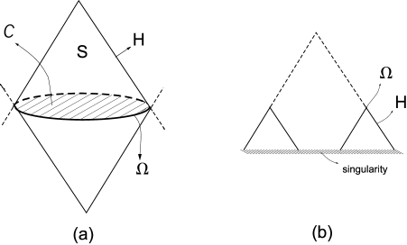
FIG. 1.: (a) The future directed light-sheet $H$ generated by a spatial one dimensional closed surface $\Omega$ in three dimensional Minkowski space. The past and future directed light-sheets bound a diamond shaped set $S$ that is causally closed. This set coincides with the causal development of a two dimensional spatial surface $C$ that is a Cauchy surface for $S$ (shaded surface). (b) Flat cosmological model with initial singularity. The figure shows a cut in the $(t,x)$ plane. A closed spatial surface $\Omega$ is represented by two points. The case shown is when this surface is bigger than the horizon, then it is antitrapped. The past directed orthogonal null congruences are light-sheets, and will crush into the singularity. The future directed ones are not light-sheets since they are initially expanding (i.e. the surface shown with the dashed line).

In a quantum field theory the Reeh-Schlieder theorem [6] impedes the discussion of the physics in a finite region in terms of subspaces of whole the Hilbert space, because the fields restricted to a bounded region generate the whole Hilbert space when acting on the vacuum . However, local algebras of operators can be defined. The diamond shaped sets of Fig. 1(a) play an important role in the algebraic approach to quantum field theory [7, 8]. In this context, to some sets $S$ in space-time it is associated an algebra ${\cal A}(S)$ of bounded operators acting on the Hilbert space ${\cal H}$, (in fact a von Neumann algebra). These have to be regarded as the algebras generated by the quantum fields averaged using weight functions with support inside the given region (see [7] for the relation with conventional quantum field theory). The operator algebras are local, in the sense that given two sets $S$, and $T$

$$S\subseteq T\Rightarrow{\cal A}(S)\subseteq{\cal A}(T)\ .$$ (1)

In addition, the operators on the algebra corresponding to the causal complement $S^{\prime}$ of $S$, ${\cal A}(S^{\prime})$, commute with the operators in ${\cal A}(S)$. Here the causal complement or opposite $S^{\prime}$ of $S$ is the set of points spatially separated from $S$. Then

$${\cal A}(S^{\prime})\subseteq{\cal A}(S)^{\prime}\ ,$$ (2)

where ${\cal A}^{\prime}$ is the algebra of the operators that commute with all the operators in ${\cal A}$.

The conditions (1) and (2) are minimal for the net of algebras, and some evolution law has to be supplemented. In Minkowski space the evolution is dictated by the existence of a unitary representation of the Poincare group acting on the local algebras. For a more general situation the dynamical law would be manifest in that for a set $S$ [7, 8]

$${\cal A}(S)={\cal A}(S^{\prime\prime})\ .$$ (3)

Then, a natural definition of the diamond shaped sets in this context, is the sets that satisfy $S=S^{\prime\prime}$. These are called causally closed sets. For example, the diamond shaped set $S$ in Fig. 1(a) is the domain of dependence $D(C)$ of the surface $C$, that is, the maximal set where it is possible to determine the variables for a wave-like theory with the knowledge of the initial data on $C$. It is also $S^{\prime\prime}=S=C^{\prime\prime}$, thus $S$ is causally closed. It was shown in [9] that the causal closure of an achronal set includes its domain of dependence, and in a globally hyperbolic space-time the domain of dependence and the causal closure coincide for achronal sets bounded in time. Therefore, eq.(3) applied to a set $S$ covering a piece of a space-like surface $C$ implies that the algebra corresponding to $S$ includes the algebra corresponding to the domain of dependence of $C$, as expected from a theory with hyperbolic equations of motion. However, eq. (3) is in general stronger than what can be induced by causal propagation (see Section III below).

We will postpone to Section III and IV the discussion of the relation between causally closed sets and the light-sheets generated by spatial codimension 2 surfaces. In this work the main discussion is centered in the geometry of the nets of causal diamond shaped sets, while its relation with the local algebras and the counting of degrees of freedom will be heuristic. We argue that under some physical conditions the net of sets to which are assigned the local operator algebras have to be taken non orthomodular. We show that this simple geometry can be associated with a possible origin of the holographic property in an effective quantum field theory description. We construct a net of causal sets that implements the cutoff in a covariant way and lead to an explanation of the non positive expansion light-sheet selection in the covariant entropy bound.

II The lattices of causally closed sets

In this Section we introduce several lattices of causal space-time subsets and briefly investigate their properties. A more extensive analysis for the orthomodular case can be consulted in [10, 11]. Given a globally hyperbolic space-time ${\cal M}$ and a set $S$ in ${\cal M}$ we call its causal opposite or orthocomplement $S^{\prime}$ to the set where the local operators in a given quantum theory are constrained to commute with the local operators in $S$. We explore several possibilities for the operation of causal opposite and its consequences for the lattices of the ”diamond shaped” (causally closed) sets. These sets are the ones that satisfy $S=S^{\prime\prime}$, and thus its definition is tied to the opposite operation.

We start with a definition for $S^{\prime}$ as the set of all points $x$ such that there is no time-like curve connecting $x$ with a point in $S$. Thus,

$$S^{\prime}=-\left(S\cup I^{+}(S)\cup I^{-}(S)\right)\,,$$ (4)

where $I^{+}(S)$ and $I^{-}(S)$ are the chronological future and past of $S$, that is, the set of points that can be reached by future directed (past directed) time-like curves starting at a point in $S$. We call ${\cal L}_{T}({\cal M})$ to the set of causally closed sets $S$, $S^{\prime\prime}=S$, where the opposite operation is given in equation (4).

Let us look more closely to the properties of ${\cal L}_{T}({\cal M})$. The empty set $\emptyset$ and ${\cal M}$ belong to ${\cal L}_{T}({\cal M})$ and are mutually complementary. It is easy to show that it is $S^{\prime\prime\prime}=S^{\prime}$ and then $S^{\prime}$ is an element of ${\cal L}_{T}({\cal M})$ for any set $S$. The operation of taking the causal opposite is internal in ${\cal L}_{T}({\cal M})$. We also have the order relation given by the set inclusion $\subseteq$. We can define two additional binary internal operations in ${\cal L}_{T}({\cal M})$, the meet $\wedge$ and the join $\vee$, given by

$$A\wedge B = A\cap B\,,$$ (5)

$$A\vee B = \left(A\cup B\right)^{\prime\prime}\,.$$ (6)

The set ${\cal L}_{T}({\cal M})$ with the order relation $\subseteq$ and the operations ^′, $\wedge$ and $\vee$, forms what is called an orthocomplemented lattice [10] (see [12, 13] for the mathematical context). A lattice ${\cal L}$ is an ordered set under some order relation $\subseteq$, where the greatest lower bound and the lowest upper bound of two elements $A$ and $B$ with respect to this order relation always exist, and are represented by the operations $A\wedge B$ and $A\vee B$ respectively. An orthocomplemented lattice has in addition a unary operation $A\rightarrow A^{\prime}$ called opposite or orthocomplement, such that

$$A \wedge A^{\prime}=\emptyset\,,$$ (7)

$$A \vee A^{\prime}=I\,,$$ (8)

$$A = A^{\prime\prime}\,,$$ (9)

$$A \subseteq B\Rightarrow B^{\prime}\subseteq A^{\prime}\,,$$ (10)

where $I$ is maximal element of the lattice (it is ${\cal M}$ for ${\cal L}_{T}({\cal M})$).

As a more familiar example of an orthocomplemented lattice we have the set ${\cal B}(U)$ of all subsets of a given set $U$. There, the order relation is again given by the inclusion $\subseteq$, while the other operations are the set complement $-$, intersection $\cap$, and union $\cup$, respectively. The properties of the operations in ${\cal L}_{T}({\cal M})$ that come from the orthocomplemented lattice structure copy those of ${\cal B}(U)$. For example, the operations $\wedge$ and $\vee$ are associative and symmetric. The duality relations also hold in any orthocomplemented lattice,

$$(A\vee B)^{\prime} = A^{\prime}\wedge B^{\prime}\,,$$ (11)

$$(A\wedge B)^{\prime} = A^{\prime}\vee B^{\prime}\,.$$ (12)

However, while the operations $\cap$, and $\cup$ are distributive in ${\cal B}(U)$, the operations $\wedge$ and $\vee$ are not distributive in ${\cal L}_{T}({\cal M})$. A similar situation occurs in the set of all closed vector subspaces of a Hilbert space, ${\cal C}({\cal H})$. The set ${\cal C}({\cal H})$ forms an orthocomplemented lattice under the order given by $\subseteq$, the opposite of a subspace $V$ given by the orthogonal space $V^{\perp}$, and the meet and join given by the intersection $\cap$, and sum $\oplus$ of vector spaces respectively. The sum and intersection do not distribute as can be checked with the vector spaces generated by three independent vectors. However, a weaker form of distributivity holds in ${\cal C}({\cal H})$ called orthomodularity, that is a central property in the studies of quantum logic [13].

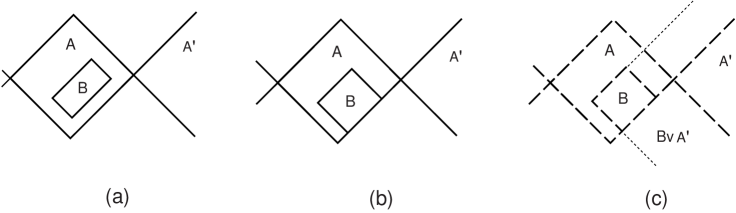
FIG. 2.: The orthomodular law is valid in ${\cal L}_{T}({\cal M})$: (a) example where $B$ is included in the interior of $A$, and (b) where $B$ is included in $A$ and share part of the border with $A$. In both cases it is $A^{\prime}\vee B=A^{\prime}\cup B$ (assuming that $A$ and $B$ do not share part of their spatial corner), and then $A\cap(B\vee A^{\prime})=B$. All sets include their time-like border. (c) The orthomodular law is not valid in ${\cal L}_{\cal O}({\cal M})$. All sets are open. The dotted line shows the set $B\vee A^{\prime}$, and it is $B\subset A\cap(B\vee A^{\prime})$. The case where $B$ is separated from the borders of $A$ is similar to (a), and orthomodularity holds for this special configurations.

It was shown in [11] for Minkowski space, and for general space-times (without imposing any causality condition) in [10] that the set ${\cal L}_{T}({\cal M})$ with the order relation $\subseteq$ and the operations $-$, $\vee$, and $\wedge$ defined above is an orthocomplemented orthomodular (and non distributive) lattice (see Fig. 2(a-b)). The orthomodularity condition is that for any $A$ and $B$ in the lattice

$$B\subseteq A\Rightarrow\,A\wedge(B\vee A^{\prime})=B\,.$$ (13)

In quantum mechanics the lattice of closed vector subspaces of the Hilbert space has a logical interpretation in terms of physical propositions, and the orthomodular property is inherent to this logic structure [13]. The proposition corresponding to a subspace $V$ on a vector state $\Psi$ is given by ”the orthogonal projection of $\Psi$ onto $V$ is $\Psi$”. Thus the answer is yes if the state vector belongs to $V$ and no if $\Psi$ belongs to the orthogonal space to $V$. The lattice of causally closed sets ${\cal L}_{T}({\cal M})$ have a logical interpretation in terms of physical propositions given by space-time subsets [10]. The proposition corresponding to a set $S$ about a point like particle is given by ”the particle passes through $S$”, while the negation of that proposition is given by ”the particle passes through $S^{\prime}$”. The prescription $S=S^{\prime\prime}$ is related with the logical axiom that states that the opposite of the opposite of a proposition gives again the same proposition. It is necessary to restrict to the causally closed sets in order to have a logic in terms of space-time sets, since for different types of sets the opposite of the corresponding proposition is a statement about particle trajectories that can not be put as a subset proposition of the above kind.

Before showing the meaning of orthomodularity in the present context we will construct a different orthocomplemented lattice of causal sets that does not have this property.

In the literature the operator algebras are usually associated with open sets, because they are thought as coming from smoothed quantum fields. It has also been suggested that the corresponding net of subsets of space-time is orthomodular [7]. The lattice ${\cal L}_{T}({\cal M})$ is orthomodular, but it is not formed by open sets. We will see that one can not have both things together.

There is another unsatisfactory feature of ${\cal L}_{T}({\cal M})$ in this context, the fact that there are orthogonal sets that can be joined by a null geodesic (see Fig. 2(b)). Here we use the term orthogonal borrowed from the lattice of closed subspaces of the Hilbert space ${\cal C}({\cal H})$ when referring to two sets $X$ , $Y$, such that $X$ $\subseteq Y^{\prime}$. Thus, as information can be passed from one set to the other the operators based on them should not necessarily commute. To take into account the propagation of massless fields one would then replace the definition of the opposite (4) by

$$S^{\prime}=-\left(J^{+}(S)\cup J^{-}(S)\right)\,,$$ (14)

where $J^{+}(S)$ and $J^{-}(S)$ are the causal future and past of $S$, that is, the set of points that can be reached from $S$ by future directed (past directed) time-like or null curves. Again an orthocomplemented lattice ${\cal L}_{C}({\cal M})$ is obtained picking up the causally complete sets $S=S^{\prime\prime}$, where the opposite operation is given by equation (14), and the meet and join by eqs. (5) and (6) [10]. Now the light rays coming from $S$ do not intersect $S^{\prime}$. However not all sets in ${\cal L}_{C}({\cal M})$ are open.

We can construct another lattice of causally closed sets where opposite sets are not causally connected, but now formed by open sets, using the opposite given by

$$S^{\prime}=-(\overline{J^{+}(S)\cup J^{-}(S)})\,,$$ (15)

and where $\bar{A}$ means the topological closure of $A$. We will call ${\cal L}_{{\cal O}}({\cal M})$ to the lattice of open sets that are causally closed with respect to the opposite operation (15). As was shown in [10], ${\cal L}_{{\cal O}}({\cal M})$ is also an orthocomplemented lattice. Both lattices ${\cal L}_{{\cal O}}({\cal M})$ and ${\cal L}_{C}({\cal M})$ behave very similarly, except that ${\cal L}_{{\cal O}}({\cal M})$ is formed by open sets and do not contain lower dimensional objects. Furthermore, in a discretized version of space-time they would coincide as explained below.

However, the lattices ${\cal L}_{{\cal O}}({\cal M})$ and ${\cal L}_{C}({\cal M})$, in contrast to ${\cal L}_{T}({\cal M})$, are not orthomodular. This is shown in the example of figure 2(c). As explained in [10] the orthocomplemented structure follows naturally from the existence of an orthogonality relation between points in space-time, but the strongest requirement of orthomodularity seems to require the exact definition (4) for the opposite.

A Some consequences of orthomodularity

There are two equivalent conditions to orthomodularity for an arbitrary orthocomplemented lattice ${\cal L}$ that we will now illustrate. The first is a kind of good property under reduction to a subspace. The lattice ${\cal L}$ is orthomodular if and only if for any $A\in{\cal L}$ the family ${\cal L}_{A}$, formed by the sets $B\in{\cal L}$, $B\subseteq A$, is again an orthocomplemented lattice, where the opposite operation restricted to ${\cal L}_{A}$ is $B\mid_{A}^{\prime}=B^{\prime}\cap A$. Then it follows that the lattice ${\cal L}_{A}$ is also orthomodular. That this condition is true for ${\cal L}_{T}({\cal M})$ and false for ${\cal L}_{{\cal O}}({\cal M})$ is exemplified in Fig. 3. What this is telling is the following. An element $A$ in ${\cal L}_{T}({\cal M})$ is not a submanifold of ${\cal M}$ because it is not an open set, but the elements of ${\cal L}_{T}({\cal M})$ inside $A$ form a good orthomodular lattice with respect to the induced operations in $A$. On the contrary, an element $A$ in ${\cal L}_{{\cal O}}({\cal M})$ is a submanifold of ${\cal M}$ because it is open, but the elements of ${\cal L}_{{\cal O}}({\cal M})$ inside $A$ are not in general elements of the lattice induced by the reduced notion of causality ${\cal L}_{{\cal O}}(A)$. The sets in ${\cal L}_{{\cal O}}({\cal M})$ included in $A$ that do not belong to ${\cal L}_{{\cal O}}(A)$ share a piece of its null border with the null border of $A$, that is, they are in contact with $A$ from inside. In fact, a weaker form of orthomodularity for ${\cal L}_{{\cal O}}({\cal M})$ holds, that reads

$$\overline{B}\subseteq A\Rightarrow\,A\wedge(B\vee A^{\perp})=B\,,$$ (16)

where $A$ and $B$ belong to ${\cal L}_{{\cal O}}({\cal M})$. The condition $\overline{B}\subseteq A$ is sufficient for $B\in{\cal L}_{{\cal O}}(A)$, but is not necessary since the examples suggest that whenever $B$ share a piece of the spatial corner with $A$ it is $B\in{\cal L}_{{\cal O}}(A)$.

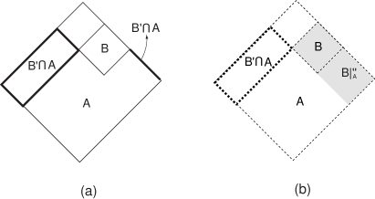
FIG. 3.: (a) The family of subsets $B\subseteq A$, where $B$ and $A$ belong to ${\cal L}_{T}({\cal M})$, form an orthomodular lattice where the opposite is given by $B\mid_{A}^{\prime}=B^{\prime}\cap A$. The figure shows the fundamental importance of the existence of null surfaces in ${\cal L}_{T}({\cal M})$ for orthomodularity. (b) With the inherited notion of the opposite for a set $A$ in ${\cal L}_{\cal O}({\cal M})$ the set $B\mid_{A}^{\prime\prime}$ (in gray) is different from $B$. Therefore $B\in{\cal L}_{\cal O}({\cal M})$ is included in $A$ but it does not belong to ${\cal L}_{\cal O}({\cal A})$.

This has a resemblance with what happens in the exterior of a black hole or in the Rindler wedge in Minkowski space where the observers can restrict themselves to living in a submanifold, but at the cost of dealing with a non pure state. Here, as we reduce to a submanifold $A$ there are sets $B$ of ${\cal M}$ included in $A$ that would have associated an algebra of local operators ${\cal A}(B)$. However, ${\cal A}(B)$ does not exist in the theory restricted to $A$ for some of the $B\subseteq A$. Thus, some local operators in $A$ would be missing from the set of operators available to the observer. Somehow the lattice ${\cal L}_{{\cal O}}({\cal M})$ would have information about the entanglement of fluctuations in the vacuum across causal horizons as implied by the Reeh-Schlieder theorem.

The second condition equivalent to orthomodularity is that for any set $S$ in an orthocomplemented lattice ${\cal L}$ there must not exist a set $T$ in ${\cal L}$ with $T\subseteq S$, $T\neq S$, and such that $T\vee S^{\prime}={\cal M}$. That is, the complement of $S^{\prime}$ is unique among the sets included in $S$. This condition is respected in ${\cal L}_{T}({\cal M})$ while it does not hold in ${\cal L}_{{\cal O}}({\cal M})$. More generally, given two orthogonal sets $A$ and $B$, and $C\subset B$, $C\neq B$, in an orthomodular lattice it can not be that $B\vee A=C\vee A$. However, this is true for certain sets in ${\cal L}_{\cal O}({\cal M})$, what could have very interesting consequences as we will see in the next Section (see Fig. 5(b)).

As the difference between the lattices presented so far is somewhat a subtlety related to the borders of the sets, one could wonder if a slight modification of the definitions would not yield a lattice of open sets orthomodular. This is not possible if one wants to retain the algebraic properties of the lattice and where the opposite consists of points spatially separated. For example a tentative possibility would be to identify the operations in ${\cal L}_{{\cal O}}({\cal M})$ with operations in ${\cal L}_{T}({\cal M})$ assigning to the set $S$ in ${\cal L}_{{\cal O}}({\cal M})$ the set $\bar{S}$ in ${\cal L}_{T}({\cal M})$. However this fails because a piece of a null surface is an element in ${\cal L}_{T}({\cal M})$ without interior, and its existence is crucial for orthomodularity (see Fig. 2(b)). Adding null surfaces to ${\cal L}_{{\cal O}}({\cal M})$ will lead to ${\cal L}_{T}({\cal M})$, that has orthogonal elements causally connected, or to ${\cal L}_{C}({\cal M})$, that is again non orthomodular.

B Models of causal lattices for a space-time with a smallest scale

A more convincing argument in favor of a non orthomodular lattice comes in a context where there is a cutoff. For example, take a discretized version of space-time choosing points at random with constant medium density with respect to the volume form, and dropping the rest of the space-time [14]. There the lattices we introduced will basically coincide, because the differences appear only when there are points lying in the same null geodesic, an event of zero probability. Call the resulting lattice ${\cal L}_{D}({\cal M})$. Also, even if it happens that two points are light connected, in any discretized version, the fact that their operators should not commute, and the points should not be orthogonal becomes strengthened in comparison with the continuum. Thus, it seems that when space-time itself is blurred at some scale (but retaining a causal relation as in [14]), extremely localized objects as the border of sets would have no meaning. The causal structure would survive at large scales through a non orthomodular causal net. We will not study here the interesting problem of finding the lattice operations of this type of discretized space-time in the thermodynamical limit. We only note that for simple examples of ${\cal L}_{D}({\cal M})$ constructed with a few points, the result is somewhat intermediate between the behavior of ${\cal L}_{\cal O}({\cal M})$ and ${\cal L}_{T}({\cal M})$ (see figure 4), a feature that we will encounter again in Section IV for a different type of regularized lattice that we now introduce.

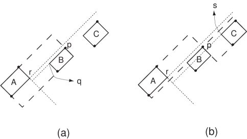
FIG. 4.: The lattice formed by choosing points at random with constant medium density in space-time and retaining the causal relations. The sets formed with the points that are in the intersection of the past and the future of two time-like separated points, as the sets $A$, $B$ and $C$, are always in the lattice. (a) There are no points inside the set bounded by the light rays passing through $q$ and $r$. Thus, the join of $A$ and $B$ is as in the lattice of open sets. (b) There is the point $p$ inside the set bounded by the light rays passing through $s$ and $r$. The set $A\vee C$ results cut by the past and future of $p$ as compared with what happens in case (a).

We mentioned that for a theory of point particles, or more generally any theory that allows to probe the space-time structure up to the continuum, the lattice ${\cal L}_{T}({\cal M})$ has an interpretation in terms of physical propositions given by space-time subsets. However, if there is a lowest scale that can be tested then the situation is different. Suppose that we can probe the space-time up to a minimal size $\mu$. We can think that our probe is an extended particle of rest frame size $\mu$. Then, given a set $S$ we can probe that a point is spatially separated from $S$ only if it is separated from $S$ by a spatial distance greater than $\mu$. Equivalently, two points will be causally unrelated if any of the extended particle trajectories passing over one point does not reach the other. Thus we define the opposite operation by

$$S^{\prime}=\{x/x\neq y\ {\hbox{and}}\ d^{2}(x,y)\leq-\mu^{2}\ {\hbox{for all}}\ y\in S\}\ ,$$ (17)

where we use the signature $(1,-1,-1,-1)$ for the metric and $d^{2}(x,y)$ is the greatest square geodesic distance between $x$ and $y$ (in case $x$ and $y$ can not be joined by any geodesic set $d(x,y)=-\infty$). The use of $\leq$ or $<$ in (17) is not relevant in what follows. A structure of orthocomplemented lattice is obtained for the causally closed sets from this definition for the opposite and we call the resulting lattice ${\cal L}_{-\mu^{2}}({\cal M})$.

We have that ${\cal L}_{-\mu^{2}}({\cal M})$ is a non orthomodular lattice, while the lattices produced by choosing a positive value instead of $-\mu^{2}$ in (17) behave as orthomodular for simple examples. The non orthomodularity of ${\cal L}_{-\mu^{2}}({\cal M})$ is in accord with the known result that given a orthocomplemented structure the orthomodularity is related with the presence of a set of states that is enough to separate the different propositions [13].

With the interpretation of the opposite of a set $S$ as the set of points where the operators commute with those based on $S$ we arrive at the same operation (17) in the case where there is a lowest fundamental scale. Operators algebras based on regions separated by a spatial distance smaller than $\mu$ may not commute because that would imply that a smaller scale have an observational significance. Only a finite number of mutually orthogonal sets are included in a given bounded diamond in the lattice ${\cal L}_{-\mu^{2}}({\cal M})$, so the net can be thought as a covariant way of implementing a cutoff because independent degrees of freedom based on different space-time sets should have commuting generators.

The causal closure (the double opposite) in ${\cal L}_{T}({\cal M})$ for an achronal bounded set has also the interpretation of being its causal domain of dependence. A similar interpretation has the closure in ${\cal L}_{-\mu^{2}}({\cal M})$. Given an orthogonal set of points $C$ in this lattice we can draw a Cauchy surface $C_{1}$ passing through all of them. Then given a point $x$ in the generated set $C^{\prime\prime}$ and any extended particle trajectory that passes over $x$, the trajectories cut $C_{1}$ at points which have a spatial distance from $C$ smaller that $\mu$. Thus, $C$ acts as a generalized form of Cauchy surface for $C^{\prime\prime}$.

Thus, it seems that the presence of a cutoff in the space-time description leads to a non orthomodular lattice for the causally closed sets that implement the causal law (3). Here the causal closure has to be calculated with the opposite (17).

From their definitions we see that ${\cal L}_{T}({\cal M})$, ${\cal L}_{C}({\cal M})$, and ${\cal L}_{{\cal O}}({\cal M})$ do not change with conformal transformations, and thus, they are a property of the conformal structure. On the contrary, ${\cal L}_{D}({\cal M})$ and ${\cal L}_{-\mu^{2}}({\cal M})$ are not conformally invariant.

III Non orthomodularity and the covariant entropy bound

We will assume that we can construct the algebra ${\cal A}(S)$ corresponding to a set $S$ formed by set union of orthogonal sets $S_{i}$ with the elements of the corresponding algebras. Thus

$${\cal A}(\cup_{i}S_{i})=\vee_{i}{\cal A}(S_{i})\ ,$$ (18)

where the sets $S_{i}$ are orthogonal, and ${\cal A}_{1}\vee{\cal A}_{2}$ denotes the algebra generated by ${\cal A}_{1}$ and ${\cal A}_{2}$. This is a natural postulate that involves a local principle. The operators associated to a set of space-like separated regions can be constructed with operators based on the given regions. However, Eq.(18) can have problems in theories with global non gauge charges (see [7], specially Section III.4). Remarkably, these charges are not supposed to survive at a fundamental level or when all effective terms in the Lagrangian are taken into account.

From eqs. (3) and (18) it follows that

$${\cal A}(\vee_{i}S_{i})=\vee_{i}{\cal A}(S_{i}),$$ (19)

for orthogonal families $S_{i}$ of elements.

Here we note that we used eq. (3) only for the union of orthogonal families of causally closed sets. Otherwise this equation can not be justified on the basis of causal propagation only. For example the double opposite of a set $S$ formed by two time-like displaced diamonds is a set bigger than the domain of dependence of $S$, that is, the set of all points through which every inextendible time-like curve intersects $S$.

Equation (19) is the statement that the local operators acting in a region of space-time can be constructed from the mutually commuting sets of operators in regions non causally connected to each other. The content of this equation clearly depends on the lattice chosen for the causally closed sets. It expresses in algebraic manner the causality of dynamical evolution due to classical space-time geometry when using the lattice ${\cal L}_{T}({\cal M})$, and it is a natural generalization for the case where the causal structure is only described by a lattice. We will proceed assuming that (19) is valid and show that it has strong implications for a non orthomodular lattice.

Now we see the role of the lattice of causally closed sets that is used as the base for the theory. In the case of ${\cal L}_{T}({\cal M})$, the picture is that of hyperbolic dynamical laws with the initial data set on Cauchy surfaces. In fact, given a diamond $S$ in ${\cal L}_{T}({\cal M})$ if we try to form it as a join of mutually orthogonal smaller diamonds, we find that these later always cover a Cauchy surface for $S$ (see Fig. 5(a)). Thus ${\cal A}(S)$ can be seen as formed by mutually commuting generators on the Cauchy surface.

The lattice ${\cal L}_{{\cal O}}({\cal M})$ implies a very different counting of degrees of freedom. As can be seen in Fig. 5(b), there each diamond is generated by a subset arbitrarily close to the spatial border of $S$, plus an arbitrarily small orthogonal diamond near one of the tips. Thus, most of the independent degrees of freedom are localized in the surface $\Omega$. When there is a cutoff the number of degrees of freedom would increase as the bounding area. The role of the non orthomodular behavior is clear. In figure 5(b) it is $A\vee C=A\vee B=S$, where $C$ is a proper subset of $B$. As already mentioned this situation can not happen in an orthomodular lattice.

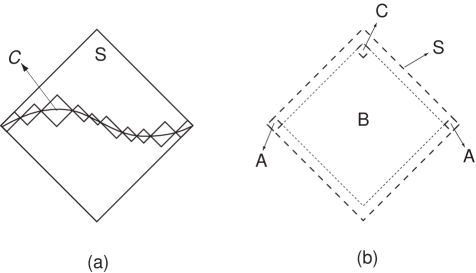
FIG. 5.: Forming $S$ as the join of mutually orthogonal sets. (a) In ${\cal L}_{T}({\cal M})$ the mutually orthogonal sets have to cover a Cauchy surface $C$ for $S$. (b) In ${\cal L}_{\cal O}({\cal M})$ it suffices to take a small set $A$ covering the spatial corner of $S$ and one orthogonal set $C$ near the future or past tip. Note that $A\vee B=A\vee C=S$.

A similar construction may be implemented for a null hypersurface converging to a point $q$, and orthogonal to a non necessarily closed codimension 2 spatial surface $\Omega$. There, a neighborhood of the null hypersurface can be formed as the join of a small set near $\Omega$ and a small orthogonal diamond near $q$.

Thus, it seems that a non orthomodular causal net captures the features of the holographic property. However, the lattice ${\cal L}_{\cal O}({\cal M})$ has two drawbacks. One is that it does not tell how to count degrees of freedom, as an arbitrarily small set in the lattice includes infinitely many orthogonal subsets. The other is that it is conformally invariant. Then, the lattice makes no difference between expanding and contracting null hypersurfaces orthogonal to $\Omega$ if they finally converge to a point. So, the same argument that applies for the surface $H$ in the case of Fig. 1(a) would apply for the dashed line representing a null hypersurface in Fig. 1(b), leading to entropy bounds with simple counterexamples (for example if the universe if big enough beyond the Hubble radius as suggested by inflation).

These difficulties can be cured using ${\cal L}_{-\mu^{2}}({\cal M})$ that implements a finite cutoff. We can give a measure of a set $S$ in this lattice that would correspond to the number of degrees of freedom available inside $S$. First, we want the independent degrees of freedom to be assigned to orthogonal sets. Second, if a set contains a pair of orthogonal subsets it can not be assigned just one degree of freedom. Thus we can think in the sets that do not contain any pair of orthogonal subsets as the building blocks. For definiteness we will take the points, that do not have any proper subsets, as such building blocks. These are the atoms of the lattice. The minimal number $N(S)$ of orthogonal points we need to generate $S$ (or a set that covers $S$ in general) is then naturally associated with some constant times the number of degrees of freedom in $S$. This definition is covariant.

As an example consider three dimensional Minkowski space, and the diamond set $S$ in Fig. 1(a). It is possible to construct the net of orthogonal points that cover the Cauchy surface $C$ as in Fig. 6(a). It also generates its domain of dependence $S$. The number of points then grows with the volume of the Cauchy surface. On the other hand, as shown in Fig. 6(b), with points near the bounding area $\Omega$ plus one single orthogonal point one can also generate a set covering $S$. The number of points is smaller than in the previous case, thus it represents the actual number (or a greater bound) of degrees of freedom.

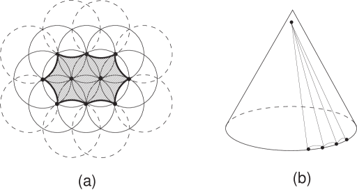
FIG. 6.: (a) Generating a spatial flat surface with a set of orthogonal points in ${\cal L}^{+}_{-\mu^{2}}({\cal M})$. The circles are of radius $\mu$. Thus the opposite of the set of points is outside the solid circles. The dashed circles are centered in the points of the opposite best positioned to take out most of the set when doing the double orthogonal. The shaded area is the set generated (or the double orthogonal) by the points, shown in the plane of the points. Here we have set the distance between neighbor points as the minimum to be orthogonal. In fact, the most efficient manner to cover the two dimensional surface is to take a hexagonal net like the shown in the picture, but where the distance between neighbors is infinitesimally near and smaller than $\sqrt{3}\mu$. When covering a surface in this way and including the time this set of points will also generate a set approximating the causal development of the surface. (b) When the radius of a circle is much bigger than $\mu$ the set formed by the central point and points in the circle will not generate a surface because some orthogonal points can be situated inside the circle. However, we can lift the central point of the circle in time, reducing its distance to the circle to the minimum $\mu$. Then, if the distance between neighbor points in the circle is less than $2\,\mu$, they will generate a set approaching a null surface. When the circle is covered, and only then, they will generate the whole cone and the lower cone also (not shown).

The reason for the holographic reduction of the number of independent degrees of freedom can be seen more easily looking at Fig.(7). Suppose we have a covariant way of assigning degrees of freedom to the Cauchy surfaces $C_{1}$ and $C_{2}$, for example by separating them by some spatial distance as we have done using the lattice ${\cal L}_{-\mu^{2}}({\cal M})$. Then, moving $C_{2}$ to approach the null boundary of $S$ its volume goes to zero reducing the number of independent degrees of freedom that the surface can hold. As both Cauchy surfaces must have the same number of independent degrees of freedom since they describe the same physics, most of the degrees of freedom of $C_{1}$ must not be independent. However, the degrees of freedom in the spatial corner may well turn out to be independent when restricting attention to the particular diamond set $S$.

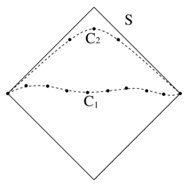
FIG. 7.: Two Cauchy surfaces $C_{1}$ and $C_{2}$ for the diamond shaped set $S$. The points represent discrete degrees of freedom equally spaced on the Cauchy surfaces. As $C_{2}$ approaches the null border of $S$ its volume tends to zero and the number of points that it can hold is reduced.

In the following Section we will give evidence in the context of a simple example that the lattice ${\cal L}_{-\mu^{2}}({\cal M})$ does indeed choose the non positive expansion condition for the applicability of the entropy bound.

IV The lattice ${\cal L}_{-\mu^{2}}({\cal M})$ for three dimensional Robertson-Walker models

In this Section we consider spatially flat three dimensional Friedman-Robertson-Walker models with a metric given by

$$ds^{2}=\eta^{\beta}\left(d\eta^{2}-dr^{2}\right)\,,$$ (20)

where $\eta$ is the conformal time, $dr^{2}=dx^{2}+dy^{2}$, and the exponent $\beta$ is taken in the range $0\leq\beta<\infty$. We focus on spatial one dimensional surfaces $\Omega$ formed by an arc of a circle at fixed $\eta$. We show that the set generated doing the double orthogonal in the lattice ${\cal L}_{-\mu^{2}}({\cal M})$ of the set formed by $A(\Omega)/(2\mu)$ orthogonal points along $\Omega$ plus a single additional orthogonal point, approximates the light sheets of negative expansion corresponding to $\Omega$ in the limit of small $\mu$. Here $A(\Omega)$ is the area of $\Omega$. On the contrary, for positively expanding null congruences orthogonal to $\Omega$ the implementation of this construction requires a greater number of points by unit surface than in the non expanding case, or it simply can not be realized with orthogonal points.

This metric (20) can be expressed in the form

$$ds^{2}=dt^{2}-a(t)^{2}dr^{2},$$ (21)

and the relation between time and conformal time is given by

$$t = \frac{\eta^{1+\frac{\beta}{2}}}{{}^{1+\frac{\beta}{2}}}\,,$$ (22)

$$a(t) = \left(\frac{1}{2}(2+\beta)t\right)^{\frac{\beta}{\beta+2}}\,.$$ (23)

From here we see that the Hubble radius $a/\dot{a}$ is given by $R_{H}=\frac{2\eta^{(1+\beta/2)}}{\beta}$. The case $\beta=0$ corresponds to flat space-time. The geodesic equation for a curve $\eta(r)$ is

$$\eta^{{}^{\prime\prime}}-\frac{\beta}{2}\eta^{-1}\left(\eta^{\prime\,2}-1\right)=0\text{.}$$ (24)

The solution for null geodesics is simply

$$\eta=\pm r+C\,,$$ (25)

where $C$ is a constant. We will be interested in small deviations from the null geodesics with $\eta$ growing with $r$, then we write

$$\eta(r)=r+C+\delta(r)\,,$$ (26)

with $\delta(r)\ll 1$. The linearized geodesic equation is

$$\delta^{{}^{\prime\prime}}-\frac{\beta}{r+C}\,\delta^{\prime}=0\text{.}$$ (27)

The solution of this equation that departs from the point $r=0$, $\eta=C$ is

$$\eta=r+C+\frac{C_{1}}{\beta+1}\left(\left(r+C\right)^{(\beta+1)}-C^{(\beta+1)}\right)\,,$$ (28)

where $C_{1}$ is a small constant, negative for space-like geodesics and positive for time-like geodesics. The square distance along these geodesics from $r=0$ to $r=r_{0}$ is

$$s^{2}=\left(\int_{0}^{r_{0}}dr\,\eta^{\frac{\beta}{2}}\sqrt{\eta^{\prime\,2}-1}\right)^{2}\,,$$ (29)

and its first order expression in $C_{1}$ is given by

$$s^{2}=\frac{2C_{1}}{(\beta+1)^{2}}\left(\left(r_{0}+C\right)^{(\beta+1)}-C^{(\beta+1)}\right)^{2}\,.$$ (30)

We have now all the elements for analyzing the following geometry. Let the spatial surface $\Omega$ be an arc of circle of radius $y_{0}$ in the plane $\eta=1$. Let $\Phi$ be the a set of points along $\Omega$ distanced $2\varepsilon$ between neighbors, where $\varepsilon$ is a small quantity of the order of the cutoff scale $\mu$, and covering in this way $\Omega$. We are assuming that the size of $\Omega$ is much greater than the cutoff $\mu$.

Take two neighbor points $p_{\pm}$ in $\Phi$, and without loss of generality assume that they have coordinates $p_{\pm}=\left(\pm\varepsilon,0,1\right)$ (see Fig. 8). The intersecting null geodesics coming from $p_{+}$ and $p_{-}$ will intersect each other at the plane $x=0$. Any pair of these intersecting null geodesic with intersection point $q$ will form the edges of a null surface $\omega$ converging to $q$ and bounded below by the sector of $\Omega$ between $p_{+}$ and $p_{-}$. Let the point $q$ be given by the coordinates $\left(0,\,y_{0},\,1+y_{0}+\varepsilon^{2}/(2y_{0})\right)$ written at second order in $\varepsilon$. Thus, $q$ is at null distance from all points in $\Phi$. The transversal area on the null surface $\omega$ at the coordinate $y$ is $2\varepsilon\frac{(y_{0}-y)}{y_{0}}(1+y)^{\beta/2}$. This is increasing for $y=0$ when $y_{0}>2/\beta=R_{H}$. In such case the null surface $\omega$ is not a light sheet in the sense of [4].

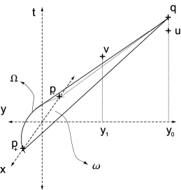
FIG. 8.: The geometry used in this Section. The points $p_{+}$ and $p_{-}$ are situated along a line parallel to the $x$ axis at $t=1$ with coordinate $x=\pm\epsilon$. Two light rays coming from $p_{\pm}$ intersect at $q$ in the plane $x=0$ at coordinate $y=y_{0}$. The point $u$ is at coordinate $y=y_{0}$ and at distance square $-\mu^{2}$ from $p_{\pm}$. The point $v$ is in the plane $x=0$, at coordinate $y=y_{1}$, and very near the null surface $\omega$.

We intend to approximate $\omega$ using the set generated by $\Phi$ and an additional point $u$ orthogonal to $\Phi$ and very near $q$. The best chance is taking $u$ to have the maximal distance square required to be orthogonal to $p_{\pm}$, $d^{2}(u,p_{\pm})=-\mu^{2}$. Using (30) with $C=1$ and $r_{0}=y_{0}$ to zero order ($C_{1}$ is already small), we obtain $C_{1}$, and replacing in (28) we have

$$u=\left(0\,\,\,\,\,,\,\,\,\,y_{0}\,\,\,\,\,\,,\,\,\,\,\,1+y_{0}+\frac{\varepsilon^{2}}{2y_{0}}-\mu^{2}\frac{(\beta+1)}{2\left((1+y_{0})^{(\beta+1)}-1\right)}\right)\,.$$ (31)

Now we want to explore the conditions under which $u$ and $\Phi$ generate a set approximating $\omega$. If we find that a point $v$, very near the surface $\omega$, belongs to the orthogonal of $\{u,\,p_{+},\,p_{-}\}$ (and then to the orthogonal of $u\cup\Phi$), then the generated set will not contain a hole in $\omega$ below or above $v$, because all past and future of $v$ is not included in $v^{\prime}$.

The form of the generated set $(u\cup\Phi)^{\prime\prime}$ will be shaped as the intersection of the opposites of the points in $(u\cup\Phi)^{\prime}$. If such a point $v$ near $\omega$ does not exist, then it can be seen that the points in $(u\cup\Phi)^{\prime}$ that could impede the generation of a set approximating $\omega$ must be near the extension of the null generators of $\omega$ beyond $\omega$. It is easy to see that if there are points in $\Phi$ along a non infinitesimal arc on each side of $p_{+}$ and $p_{-}$, there are no points in $(u\cup\Phi)^{\prime}$ near the null generators of $\omega$ extended at the future of $\omega$. Therefore, in the case no such a point $v$ can be found, a point near $\omega$ will be generated for each $y$ between $0$ and $y_{0}$.

Thus, we search points $v$ capable of making holes in the generated set, and we situate $v$ with a coordinate $y=y_{1}$ and on the plane $x=0$. The reason for this last election is that the distance from $u$ is the same in the whole arc of radius $y_{0}-\,\,y_{1}$ around $y_{0}$, while if one chooses a point $v$ with some $x\neq 0$ there is less distance square to one of the points $p_{+}$ or $\,p_{-}$ and more to the other. Thus, as the distance square from $v$ to both has to be less than $-\mu^{2}$, the best chance is with $x=0$. Points $v$ displaced along the $x$ direction beyond the surface $\omega$ can be orthogonal to $p_{+}$ and $p_{-}$, but they are taken into account in the next patch of null surface corresponding to other points in $\Phi$.

Thus we choose

$$v=\left(0\,\,\,\,\,,\,\,\,\,\,y_{1}\,\,\,\,\,,\,\,\,\,\,1+y_{1}+\frac{\varepsilon^{2}}{2y_{0}}+\Delta\right)\,,\,$$ (32)

where $\Delta$ is a small quantity and $0<y_{1}<y_{0}$. Using (28) and (30) we obtain the distance square $d^{2}(v,p_{\pm})$ that is given by

$$d^{2}(v,p_{\pm})=-\frac{2}{(\beta+1)}\left((1+y_{1})^{(\beta+1)}-1\right)\left(\varepsilon^{2}\frac{(y_{0}-y_{1})}{2y_{1}y_{0}}-\Delta\right)\,.$$ (33)

Likewise, we compute the distance square between $v$ and $u$,

$$d^{2}(v,u)=-\frac{2}{(\beta+1)}\left((1+y_{0})^{(\beta+1)}-(1+y_{1})^{(\beta+1)}\right)\left(\frac{\mu^{2}(\beta+1)}{2\left((1+y_{0})^{(\beta+1)}-1\right)}+\Delta\right)\text{.}$$ (34)

As mentioned, for making holes in the generated set we have to demand $d^{2}(v,p_{\pm})\leq-\mu^{2}$ and $d^{2}(v,u)\leq-\mu^{2}$. These translates into the following conditions for $\Delta$

$$\varepsilon^{2}\frac{(y_{0}-y_{1})}{2y_{1}y_{0}}-\frac{\mu^{2}(\beta+1)}{2\left((1+y_{1})^{(\beta+1)}-1\right)}\geq\Delta\,,$$ (35)

$$\Delta \geq \mu^{2}\frac{(\beta+1)}{2}\left[\frac{1}{\left((1+y_{0})^{(\beta+1)}-(1+y_{1})^{(\beta+1)}\right)}-\frac{1}{\left((1+y_{0})^{(\beta+1)}-1\right)}\right]\,.$$ (36)

Given $\beta$ and $y_{0}$ we have to satisfy these conditions for $y1\in[0\,,\,y_{0}]$. Thus, $\Delta\geq 0$. If a point $v$ is in $\{u,$ $p_{+},\,p_{-}\}^{\prime}$, then all the points in the null surface $\omega$ for $x=0$ and smaller $y$ will be time like connected with $v$ and will not be in the generated set.

The condition for the existence of $\Delta$ can be restated as

$$\frac{1}{\left((1+y_{0})^{(\beta+1)}-1\right)}-\frac{1}{\left((1+y_{1})^{(\beta+1)}-1\right)}-\frac{1}{\left((1+y_{0})^{(\beta+1)}-(1+y_{1})^{(\beta+1)}\right)}$$ (37)

$$+\frac{\varepsilon^{2}}{\mu^{2}}\frac{(y_{0}-y_{1})}{(\beta+1)\,y_{1}y_{0}}\geq 0\,.$$ (38)

For a given $\beta>0$, taking $y_{0}\rightarrow\infty$, $y_{1}\rightarrow\infty$, and $y_{0}/y_{1}\rightarrow\infty$, we see that there are always solutions for any $\varepsilon$ when the surface is big enough. Thus, surfaces with big $y_{0}$ are not generated given a fixed $\varepsilon$. For $\varepsilon>\mu$ we have points in $(u\cup\Phi)^{\prime}$ in the initial surface and a set converging to $\omega$ for small $\mu$ will not be generated. Let us take the minimal set of orthogonal elements in the spatial surface that do not admit the addition of other orthogonal points, that is, we take $\varepsilon$ to be an infinitesimal smaller than $\mu$. With such a choice the function (38) is decreasing with $y_{1}$. Then it suffice to take the limit $y_{1}\rightarrow 0$. There the condition (38) becomes

$$y_{0}\geq\frac{2}{\beta}\text{. }$$ (39)

Therefore, for expanding surfaces, the number of orthogonal points required in the spatial surface $\Omega$ to generate the approximate null surface will be greater than the minimal orthogonal set of points that cover (but not generate by themselves) the surface $\Omega$ [16]. This does not happen for contracting surfaces, where it suffices with taking $A(\Omega)/(2\mu)$ points on the surface $\Omega$ of area $A(\Omega)$.

For $\mu/2\leq\varepsilon<\mu$ we can still generate the set converging to $\omega$ in certain range of $y_{0}$, with the point $u$ plus orthogonal points in the initial surface, leading to an extension of the holographic idea, but where the number of degrees of freedom per unit area is increased with respect to the standard value applicable to the non expanding case. For a large enough $y_{0}$ it is not possible to choose $\varepsilon$ in this range to generate the surface. Of course it can still be generated with non orthogonal points, for small enough $\varepsilon$. Numerically, certain conservation of the number of points seems to hold. For a given $y_{0}$ let $\hat{\varepsilon}$ be the maximal $\varepsilon$ such that there exist no $y_{1}$ such that Eq.(38) holds. Then let the area of maximal expansion for the initial surface of area $2\,\hat{\varepsilon}$ be $A_{\max}(2\,\hat{\varepsilon})$. It is $A_{\max}(2\,\hat{\varepsilon})/(2\,\mu)\simeq 1$. Therefore the number of points needed in the surface $\Omega$ (in general non orthogonal points) is very similar to the minimal number of orthogonal points needed to cover the surface of maximal expansion.

We hope that an analysis on the same line involving the geodesic deviation equation would yield the result of this Section on the relation between the covariant entropy bound and the geometry given by the lattice ${\cal L}_{-\mu^{2}}({\cal M})$, in a more general context.

V Conclusions

We have seen, considering the geometry of classical space-time, that there exist two well differentiated classes of orthocomplemented nets of causal sets. One is given by the orthomodular net ${\cal L}_{T}({\cal M})$, which is related to the usual picture of using independent data on Cauchy surfaces. The other class is of non orthomodular nets, that can be related to a reduction of degrees of freedom of the holographic type. We have argued that the second type of nets should be used for constructing algebraic quantum theories if there is a cutoff scale.

Somewhat at the extreme of the non orthomodular behavior is the lattice ${\cal L}_{\cal O}({\cal M})$, that, being conformally invariant, does not differentiate between contracting and expanding light-sheets. When regularizing the lattices one takes into account the metric in addition to the causal structure, and the resulting behavior is intermediate between ${\cal L}_{T}({\cal M})$ and ${\cal L}_{\cal O}({\cal M})$.

We have constructed the non orthomodular lattice ${\cal L}_{-\mu^{2}}({\cal M})$ that implements a covariant cutoff for the causal lattices. This allows a geometrical definition of the number of degrees of freedom for an arbitrary set in space-time. We have seen that this number is consistent with the Bousso covariant entropy bound in a simple example, where it reproduces the non negative expansion condition for the election of light-sheets.

An important point suggested by the lattices constructed in this work is that while the covariant entropy bound would hold in its original form, the holographic projection for a diamond shaped set or a light sheet would not be simply to degrees of freedom on the spatial bounding surface. These are most of the independent degrees of freedom, but something more seems to be needed along the light sheet or its tip to close the algebra.

The lattice ${\cal L}_{T}({\cal M})$ can be taken as a description of the causal structure in classical space-time [10]. It is othomodular and it also has an interpretation in terms of physical propositions for classical theories. As we have argued the corresponding object that describes causality when space-time can not be taken classical at all the scales should be a non orthomodular lattice. If the causal propositions remain physical propositions that would mean that orthomodularity is lost as a property of the quantum logic structure. A change of the quantum mechanics postulates in a cosmological scenario is advocated for example in Ref.[15].

It would be interesting to explore the purely geometrical problem posed by the lattice ${\cal L}_{-\mu^{2}}({\cal M})$. Does it reproduces the holographic property for a general space-time?. A precise formulation for this statement is the following. Given a codimension 2 spatial surface $\Omega$ and one of its light-sheets $H$, and let $N(S)$ be the minimal number of orthogonal points needed to generate a set covering $S$ in space-time. Then we would like to test if $\lim_{\mu\rightarrow 0}\frac{N(\Omega)}{N(H)}=1$, or find the conditions for its validity.

More generally, the lattice ${\cal L}_{-\mu^{2}}({\cal M})$ suggests a generalized geometrical version of entropy bound. This is simply that the entropy in a set $S$ has to be less than a constant times $N(S)$. The constant has to be adjusted to match the covariant bound when appropriate, and is given by $3\sqrt{3}\mu^{2}/(8G)$ in four dimensions [16]. Thus, this geometrical bound would be independent of $\mu$ when the cutoff is taken smaller than all the curvature scales in the set.

In relation to this idea arises the question of what kind of regularization could lead to the stronger form of covariant entropy bound given in [5], which is related to the Bekenstein entropy bound [17], and implies the generalized second law. This can not be deduced from the counting of degrees of freedom by the lattice ${\cal L}_{-\mu^{2}}({\cal M})$.

It would also be interesting to investigate other regularizations, as the given by the lattice resulting from a random distribution of points in space-time ${\cal L}_{D}({\cal M})$ in the thermodynamical limit.

Here we have assumed a base classical space-time and a net of local algebras of operators in Hilbert space as a generalized form of quantum field theory. This structure should appear above some distance scale. What seems to be odd is that, following what we have argued, the covariant entropy bound would hold in a form logically independent of the Einstein equations for the metric. After all the Einstein equations are essential for curving the space in such a way to save the bound in several examples [4, 5]. However, the order of the implications could possibly be inverted using an idea by Jacobson [18]. In that work the Einstein equations are deduced starting from the area law for the entropy, and using the second law of thermodynamics as seen by accelerated observers to relate a heat flux given by the stress tensor with the area expansion. Thus, it seems likely that to implement an effective theory valid above some smallest fundamental scale gravity should appear as a requirement of self consistency.

- [1] R.M. Wald, Living Rev. Rel. 4, 6 (2001), gr-qc/9912119.
- [2] G. ’t Hooft, Dimensional reduction in quantum gravity, gr-qc/9310026 ; L. Susskind, J. Math. Phys. 36, 6377 (1995), hep-th/9409089 ; J.D. Bekenstein, Do we understand black hole entropy? , gr-qc/9409015.
- [3] R. Bousso, The holographic principle, hep-th/0203101.
- [4] R. Bousso, JHEP 07, 004 (1999), hep-th/9905177; JHEP 06, 028 (1999), hep-th/9906022; Class. Quant. Grav. 17, 997, hep-th/9911002. For a previous related work see: W. Fischer and L. Susskind, Holography and cosmology, hep-th/9806039.
- [5] E.E Flanagan, D. Marolf and R.M. Wald, Phys. Rev. D62, 084035 (2000), hep-th/9908070.
- [6] H. Reeh and S. Schlieder, Nuovo Cimento 22, 1051 (1961) (original article in German). English versions appear in the book of Ref. [7] and in Axiomatic Quantum Field Theory, N.N. Bogoluvov, A.A. Logunov and I.T. Todorov (W.A. Benjamin Inc., Reading, 1975). A generalization to curved spaces is in A. Strohmaier, R. Verch and M. Wollenberg, Microlocal analysis of quantum fields on curved space-times: Analytic wavefront sets and Reeh-Schlieder theorems, math-ph/0202003.
- [7] Local quantum physics, R. Haag (Springer-Verlag, Berlin, 1992). Some works on extensions of the formalism to general space-times are in [8].
- [8] J. Dimock, Commun. Math. Phys. 77, 219 (1980); R. Brunetti, K. Fredenhagen, and R. Verch, The generally covariant locality principle - A new paradigm for local quantum physics, math-ph/0112041. For works on the holographic principle in the context of algebraic quantum field theories see K.H. Rehren, Annales Henri Poincare 1, 607 (2000), hep-th/9905179; B. Schroer, The paradigm of the area law and the structure of transversal-longitudinal lightfront degrees of freedom, hep-th/0202085. For a recent review and further references see D. Buchholz, Algebraic quantum field theory: a status report, math-ph/0011044.
- [9] W. Cegla and J. Florek, Causal logic with physical interpretation, Univ. Wroclaw Pp. 524 (1981).
- [10] H. Casini, Class. Quantum Grav. 19, 1 (2002); qr-qc/0205013.
- [11] W. Cegla and A.Z. Jadczyk, Comm. Math. Phys. 57, 213 (1977) ; Orthomodularity of causal logics, W. Cegla and J. Florek, preprint 471, Univ. Wroclaw Pp. 262, 265 (1979).
- [12] G.Birkhoff, Lattice Theory (American Mathematical Society Colloquium Publications, vol XXV, Providence, 1967) ; Orthomodular lattices, G. Kalmbach (Academic Press, London, 1983).
- [13] Quantum Logic, P.Mittelstaedt (D. Reidel Publishing Company, Dordrecht, 1978) ; The logic of quantum mechanics, E.G. Beltrametti and G. Cassinelli (Addison Wesley Publishing Company, Reading, 1981).
- [14] L. Bombelli, J. Lee, D. Meyer, and R.D. Sorkin, Phys. Rev. Lett. 59, 521 (1987); Phys. Rev. Lett. 60, 656 (1988). See for a recent work D. Dou, Ph.D. Thesis, Trieste, SISSA (1999), gr-qc/0106024, and references therein.
- [15] V. Balasubramanian, J. de Boer, and D. Minic, Holography, time and quantum mechanics, gr-qc/0211003. However, for a different perspective where the continuum is not lost see H. Casini, Finite dimensions and the covariant entropy bound, hep-th/0211253.
- [16] To find the optimal distribution of points in a two-dimensional sphere in such a way of maximizing the minimal distance between points is an interesting open problem in mathematics. For the plane it is given by the hexagonal net. For the sphere or any other surface, if the cutoff scale is much smaller than the curvature radius, it will be given by an hexagonal net almost everywhere. See M. Berger, La Recherche 346, 38, oct. (2001).
- [17] J.D. Bekenstein, Phys. Rev. D23, 287 (1981). R. Bousso, Light-sheets and the Bekenstein’s bound, hep-th/0210295.
- [18] T. Jacobson, Phys. Rev. Lett. 75, 1260 (1995), qr-qc/9504004.