Naked Singularity and Thunderbolt

Abstract

We consider quantum theoretical effects of the sudden change of the boundary conditions which mimics the occurrence of naked singularities. For a simple demonstration, we study a massless scalar field in $(1+1)$-dimensional Minkowski spacetime with finite spatial interval. We calculate the vacuum expectation value of the energy-momentum tensor and explicitly show that singular wave or thunderbolt appears along the Cauchy horizon. The thunderbolt possibly destroys the Cauchy horizon if its backreaction on the geometry is taken into account, leading to quantum restoration of the global hyperbolicity. The result of the present work may also apply to the situation that a closed string freely oscillating is traveling to a brane and changes itself to an open string pinned-down by the ends satisfying the Dirichlet boundary conditions on the brane.

^† Yukawa Institute for Theoretical Physics,
Kyoto University,
Kyoto 606-8502, Japan

^‡ Department of Physics,
Tokyo Institute of Technology,
Oh-Okayama Meguro-ku, Tokyo 152-0033, Japan

1 Introduction

A question of whether the cosmic censorship holds is one of the most important issues in classical general relativity, but still remains far from being settled. Many attempts have so far been made to prove the validity of this conjecture and have achieved partial success under some particular setup. On the other hand, some of those attempts have resulted in rather showing the counter examples, indicating that the classical framework of general relativity admits appearance of naked singularities (See e.g., Review [1]). In the present situation of research on the cosmic censorship hypothesis described above, it is probably more sensible to classify naked singularities and ask whether it is a disastrous one for physics or a practically harmless one.

In the previous work [2], as a physically sensible classification of naked singularities, we proposed the wave approach to probe naked singularities. There, we studied the wave propagation in various static spacetimes with naked singularities. The essential point was the uniqueness of self-adjoint extension of the time-translation operator $A$, defined by the spatial derivatives in the wave equation. We call the classical singularity wave-regular if the self-adjoint extension is unique, i.e., there is no ambiguity in the boundary condition at the singularity. In the wave-regular case, thus there exists a unique solution to the wave equation for a given initial value; the predictability holds at least for the probe fields even in the classical framework. In this sense, the concept of wave-regularity is closely related to Clarke’s idea of generalised hyperbolicity [3].  Such a would-be singularity can be regarded as a harmless singularity. On the other hand, if the time evolution of an initial value is not unique so that the predictability for a probe wave field breaks down, such a naked singularity is called wave-singular.

The idea of the wave probe rather than particle probe is based on semi-classical theory, in which geometry is treated classically but matter fields quantum mechanically, with the probe waves identified with the mode functions for quantum fields. One might anticipate that, once a theory of quantum gravity is established, one would not need be afraid of the emergence of naked singularities; a naked singularity could be resolved by replacing it with something like a boundary of Planck energy scale, and in the neighborhood of the resolved singular boundary, the predictability of physics would be restored quantum mechanically. But even in such a case, a remaining question will be how such an extremely high energy boundary looks like from distant observers who live in a low energy scale governed by (semi-) classical theories. Then, it seems plausible that a naked ‘singularity’ resolved by any kind of quantum gravitational theory looks wave-regular from distant observers, as the wave-regularity respects the predictability of low energy (semi-) classical physics. In this sense, naked singularities can be classified into two types: one of which can be resolved to be wave-regular by quantum gravity, while the other should be somehow prohibited.  Here, we would like to propose a version of (quantum-) cosmic censorship advocating that, in semi-classical theory, wave-singular naked singularities are prohibited to appear by quantum field theoretical effects.

In the present work, aiming at examining the above version of quantum cosmic censorship, we shall focus our attention on the wave-singular case in which a timelike singularity emerges at some stage and the boundary condition is not a priori specified. This feature may manifest itself when the singularity appears in occasion of gravitational collapse. A simplified version will be the case that the boundary condition suddenly changes at some time so that the boundary becomes a naked timelike singularity.

We shall consider such a case in the context of quantum field theory. The time-translation operator $A$ for a field changes in time by the change of its domain ${\cal D}(A)$ so that we naturally expect particle creations from a vacuum state of the field. We shall first show that this is indeed the case in the perhaps simplest example: a massless scalar field theory in a $(1+1)$-dimensional spacetime ${\mathbb{R}}\times[0,\pi]$, with the boundary condition at $0$ and $\pi$ suddenly changing from the Neumann to the Dirichlet boundary condition. We shall compute the vacuum expectation value of the energy-momentum tensor and see that it just gives the standard Casimir energy inside the domain of dependence while it is divergent at the Cauchy horizon for the initial hypersurface $\{0\}\times[0,\pi]$. We will observe the thunderbolt effect [7] in the sense that there appears a delta function like singularity which has a support only on the Cauchy horizon. If the backreaction on the geometry is taken into account, the thunderbolt effects will destroy the Cauchy horizon, resulting in quantum mechanical restoration of the global hyperbolicity. We shall also give discussion for the general boundary conditions case in the appendix.

Long ago Anderson and DeWitt [8] discussed a similar problem in the context of topology change in spacetime which exhibits a splitting of the compact universe like ‘trousers.’ They discussed particle creations with an infinite amount of energy which appear an infinitely bright flash emanating from the crotch of the trousers. In a sense the emergence of a naked singularity is a kind of topology change which alters the domain of definition for quantum fields. Not surprisingly their result, which is not fully quantitatively described, is qualitatively very similar to ours.

It is interesting to point out a possible application to string and brane theories [9]. In the brane picture of universe, an open string can propagate along a brane with both the ends satisfying the Dirichlet boundary conditions on the brane but also can pinch off from the brane to the bulk spacetime as a closed string. In that process the boundary condition at the ends changes. The emerged closed string will be highly excited because of the sudden change of the boundary condition as an analog of the phenomenon described in the present work.

2 Hair of wave-singular naked singularity

For self-containedness we briefly recapitulate the self-adjoint extension of the time-translation operator in a static spacetime case. The relevant mathematical materials are collected in the appendix of Ref. [2]. For thorough study of this issue, see Ref. [10].

When probing timelike singularities in a static spacetime with a scalar wave $\phi$, the wave equation can take the form

$$\frac{\partial^{2}}{\partial t^{2}}\phi=-A\phi\,,$$ (1)

where $t$ is the Killing time and $A$ denotes an operator containing only spatial coordinates and derivatives. We will find the preliminary time-translation operator $A$ as a symmetric operator on a given Hilbert space $\cal H$ with domain $C^{\infty}_{0}$, a set of smooth functions with compact support on $t=const.$ surface. A trivial symmetric extension is immediately made by taking its closure. Consider then the sets ${\cal K}_{\pm}:=\{\phi_{\pm}\in{\cal H}|A^{*}\phi_{\pm}=\pm i\phi_{\pm}\}$, which are called the deficiency subspaces of $A$, and the pair of numbers $(n_{+},n_{-}):=(\dim{\cal K}_{+},\dim{\cal K}_{-})$ called the deficiency indices of $A$. If $A$ with domain ${\cal D}(A)$ is a closed symmetric operator with $n_{+}=n_{-}$, then $A$ has self-adjoint extensions. Let $U$ be the partial isometries ${\cal K}_{+}\rightarrow{\cal K}_{-}$. Then the self-adjoint extensions ${A_{E}}$ can be obtained by taking the domain as [10]

$${\cal D}({A_{E}}):=\{\phi_{0}+\phi_{+}+U\phi_{+}\,|\,\phi_{0}\in{\cal D}(A),\,\phi_{+}\in{\cal K}_{+}\}.$$ (2)

Given self-adjoint extension $A_{E}$, dynamics of the scalar field $\phi$ for any initial data $(\phi(0),\partial_{t}\phi(0))\in{\cal H}\times{\cal H}$ can be defined as

$$\phi(t)=\cos\left(\sqrt{A_{E}}t\right)\;\phi(0)+\frac{1}{\sqrt{A_{E}}}{\sin\left(\sqrt{A_{E}}t\right)}\;{\partial\over\partial t}{\phi}(0).$$ (3)

The point is that, once a self-adjoint extension is given, the vector $\phi(t)\in{\cal H}$ is defined not only inside the future domain of dependence for the initial hypersurface but also even outside the domain of dependence [11].

In general, self-adjoint extension is not necessarily unique, when spacetime fails to be globally hyperbolic. Even when spacetime admits naked singularities, if $n_{+}=n_{-}=0$, then $A$ has a unique self-adjoint extension and dynamics of the probe field is uniquely determined everywhere from the initial data by Eq. (3). This case is referred to as wave-regular. If $n_{+}=n_{-}=N\neq 0$, then the partial isometry $U$ is represented by an $N\times N$ unitary matrix $U(N)$, and $A$ has infinitely many different self-adjoint extensions, which are in one-to-one correspondence with $U(N)$. In this case the naked singularity is called wave-singular. Each self-adjoint extension corresponds to the different boundary condition at the singularity and accordingly describes different time evolution of the wave for the same initial data. In other words, a wave-singular naked singularity has degrees of freedom for the possible choice of the time-translation operator $A_{E}$. The degrees of freedom can be interpreted as the character or the hair of the wave-singular naked singularity, described by the isometries $U(N)$. For example, when a scalar probe field is considered in $(1+1)$-dimensions of the finite spatial interval with the wave-singular singularities at both the ends, the hair of the singularities is $U(2)$.

It should be commented that the wave-regularity depends on the choice of our Hilbert space $\cal H$. As emphasized in Ref. [2], the Sobolev space, which requires $L^{2}$ of the derivatives of $\phi$ as well as $\phi$ itself, will provide a physically sensible Hilbert space for the singularity probe. In the present work, however, as a simple illustration, we shall take $L^{2}$-space of square integrable functions as adopted in Ref. [12]. The analysis in the next section can be straightforwardly generalized to the Sobolev space case. The results will somewhat change depending on the choice of the Hilbert space.

3 Quantum behavior of a probe field

3.1 A simple model

In this section, as one of the simplest cases, we shall consider a quantum field theory of a massless scalar field in $(1+1)$-dimensional Minkowski spacetime ${\mathbb{R}}\times[0,\pi]\ni(t,x)$. As mentioned before, the hair for the boundary “singularities” in this case becomes the group $U(2)$, but here we shall consider only its subgroup $U(1)\times U(1)$ with each $U(1)$ corresponding to the arbitrariness of the boundary conditions at $x=0,\,\pi$, respectively. We are concerned with quantum field theoretical effects in the situation that the hair $U(1)\times U(1)$ suddenly changes at some time, say $t=0$, which can be interpreted as a sudden appearance of wave-singular timelike singularities at $x=0,\,\pi$ for $t>0$.

The scalar field $\phi$ obeys the Klein-Gordon equation (1) with an elliptic operator

$$\quad\quad A:=-\frac{\partial^{2}}{\partial x^{2}}\,.$$ (4)

We require the square integrability for the scalar field, i.e., $\phi\in L^{2}(0,\pi)=\{\phi\,|\,\int^{\pi}_{0}dx|\phi|^{2}<\infty\,\}$, so that we can regard $A$ with ${\cal D}(A)=C^{\infty}_{0}(0,\pi)$ as a positive symmetric operator in the Hilbert space $L^{2}(0,\pi)$ with the inner product,

$$(\phi_{1},\,\phi_{2}):=\int^{\pi}_{0}\!dx\;\phi_{1}^{*}(x)\phi_{2}(x)\,.$$ (5)

Then, having a suitable self-adjoint extension $A_{E}$ of $A$, we can obtain the solution for any initial data $(\phi(0,x),\,\partial_{t}{\phi}(0,x))$ from Eq. (3).

We shall focus on a particular situation that the boundary conditions at $x=0,\,\pi$ are the Neumann boundary conditions, $\partial\phi/\partial x=0$, before $t=0$ but switch to the Dirichlet boundary condition, $\phi=0$ at $x=0,\,\pi$, after $t=0$. This sudden change of the boundary conditions can be viewed as a particular case of the occurrence of wave-singular naked singularities at $x=0,\,\pi$ after $t=0$.

3.2 Mode functions

Before $t=0$ the positive frequency mode functions satisfying the Neumann boundary condition at $x=0,\,\pi$ are given by

$$f^{(in)}_{n}(t,x) = \frac{e^{-int}}{\sqrt{\pi n}}\cos nx\,,\quad(n=1,2,\cdots)\,,$$ (6)

which are normalized by the Klein-Gordon inner product: $i\left\{(f,\;\partial_{t}g)-(\partial_{t}f,\;g)\right\}$. Then we can expand the field $\phi(t,x)$ for $t<0$ as

$$\phi(t,x)=f_{0}(t,x)+\sum_{n=1}^{\infty}\left\{a^{(in)}_{n}f^{(in)}_{n}(t,x)+{a^{(in)}_{n}}^{\dagger}{f^{(in)}_{n}}^{*}(t,x)\right\}\,,$$ (7)

where

$$f_{0}(t,x)=\frac{1}{\sqrt{\pi}}(q+p\;t)\,,$$ (8)

is the zero-mode. The expansion coefficients are required to satisfy the canonical commutation relations

$$\left[a^{(in)}_{n},\;{a^{(in)}_{n^{\prime}}}^{\dagger}\right]=\delta_{nn^{\prime}}\,,\quad\left[a^{(in)}_{n},\;a^{(in)}_{n^{\prime}}\right]=\left[{a^{(in)}_{n}}^{\dagger},\;{a^{(in)}_{n^{\prime}}}^{\dagger}\right]=0\,,\quad\left[q,\,p\right]=i\,,$$ (9)

and $a^{(in)}_{n}$, ${a^{(in)}_{n}}^{\dagger}$ commute with $q$ and $p$ so that the canonical quantization is reproduced:

$$\left[\phi(t,x),\;\partial_{t}\phi(t,x^{\prime})\right]=i\delta(x-x^{\prime})\,.$$ (10)

Now let us consider the time evolution of $\phi(t,x)$ into the future ($t>0$) region of the initial surface $t=0$, where the probe field $\phi(t,x)$ is supposed to satisfy the Dirichlet boundary condition $\phi(t,0)=\phi(t,\pi)=0$, and accordingly the positive frequency mode functions are given by

$$f^{(out)}_{m}(t,x)=\frac{e^{-imt}}{\sqrt{\pi m}}\sin mx\,.$$ (11)

In order to study the time evolution of $\phi$ into $t>0$ region, we need to modify the initial data at $t=0$ so as to fit the Dirichlet boundary condition. We shall discuss the positive frequency modes $f^{(in)}_{n}$ and the zero-mode $f_{0}$ separately.

First, using the Fourier expansion,

$$\cos nx=\sqrt{\frac{2}{\pi}}\sum_{\stackrel{{\scriptstyle m=1}}{{(m\pm n:odd)}}}^{\infty}\left(\frac{1}{m+n}+\frac{1}{m-n}\right)\;\sin mx\,,$$ (12)

we can express the initial data of the positive frequency modes as

$$f^{(in)}_{n}(0,x) = \frac{1}{\pi}\sqrt{\frac{2}{n}}\sum_{\stackrel{{\scriptstyle m=1}}{{(m\pm n:odd)}}}^{\infty}\left(\frac{1}{m+n}+\frac{1}{m-n}\right)\;\sin mx\,,$$ (13)

$${\partial\over\partial t}f^{(in)}_{n}(0,x) = -in\;f^{(in)}_{n}(0,x)\,.$$ (14)

The evolution of the mode function $f^{(in)}_{n}$ into $t>0$ region is obtained by inserting the above initial data (13) and (14) into Eq. (3), in which ${\cal D}(A_{E})$ is now spanned by the basis $\{f^{(out)}_{m}\}$ so as to respect the Dirichlet boundary condition. Then we can find

$$f^{(in)}_{n}(t,x) = \sum_{m=1}^{\infty}\left\{\alpha_{nm}\;f^{(out)}_{m}(t,x)+\beta_{nm}\;{f^{(out)}_{m}}^{*}(t,x)\right\}\,,$$ (15)

with the coefficients

$$\alpha_{nm} = \frac{2}{\pi}\sqrt{\frac{m}{{}\;n{}\;}}\;\frac{1}{m-n}\delta_{m\pm n:odd}\;,\quad\beta_{nm}=\frac{2}{\pi}\sqrt{\frac{m}{{}\;n{}\;}}\;\frac{1}{m+n}\delta_{m\pm n:odd}\;,$$ (16)

where and hereafter $\delta_{m\pm n:odd}$ means $\delta_{m\pm n:odd}=1$ if $m\pm n=\mbox{an odd number}$ and $\delta_{m\pm n:odd}=0$ otherwise.

The consistency of the canonical commutation relations (9) requires the unitarity relation

$$\sum_{n=1}^{\infty}\left(\alpha_{nm}\alpha^{*}_{nm^{\prime}}-\beta^{*}_{nm}\beta_{nm^{\prime}}\right)=\delta_{mm^{\prime}}\,.$$ (17)

This can be checked by using the formula

$$\sum_{\stackrel{{\scriptstyle n=1}}{{(n:odd)}}}^{\infty}\frac{1}{n^{2}}=\frac{\pi^{2}}{8}\,.$$ (18)

Next, let us expand the mode which is the time evolution after $t=0$ of the zero-mode before $t=0$ in terms of the late time mode functions (11) as

$$f_{0}(t,x)=\sum^{\infty}_{m=1}\left\{C_{m}f^{(out)}_{m}(t,x)+C_{m}^{\dagger}{f^{(out)}_{m}}^{*}(t,x)\right\}\,.$$ (19)

The initial data is then given by

$$f_{0}(0,x) = \sum^{\infty}_{m=1}(C_{m}+C_{m}^{\dagger})\frac{\sin mx}{\sqrt{\pi m}}=\frac{q}{\sqrt{\pi}}\,,$$ (20)

$${\partial\over\partial t}f_{0}(0,x) = \sum^{\infty}_{m=1}(-im)(C_{m}-C_{m}^{\dagger})\frac{\sin mx}{\sqrt{\pi m}}=\frac{p}{\sqrt{\pi}}\,,$$ (21)

by continuity at $t=0$. Then, by using the formula: $(\sin mx,\sin nx)=\frac{\pi}{2}\delta_{m,n}$, the expansion coefficients are obtained as

$$C_{m}=\frac{2}{\pi}\frac{1}{\sqrt{m}}\left(q+\frac{i}{m}p\right)\delta_{m:odd}\,.$$ (22)

3.3 Particle creations

Suppose the quantum field $\phi$ is expanded in terms of the (out)-mode functions as

$$\phi(t,x) = \sum_{m}\left\{a^{(out)}_{m}f^{(out)}_{m}(t,x)+{a^{(out)}_{m}}^{\dagger}{f^{(out)}_{m}}^{*}(t,x)\right\}\,.$$ (23)

Then, from Eqs. (7), (15), and (19), we have the Bogoliubov transformation

$$a^{(out)}_{m} = C_{m}+\sum_{n}\left\{\alpha_{nm}a^{(in)}_{n}+\beta_{nm}{a^{(in)}_{n}}^{\dagger}\right\}\,,$$ (24)

$${a^{(out)}_{m}}^{\dagger} = C^{\dagger}_{m}+\sum_{n}\left\{\alpha^{*}_{nm}{a^{(in)}_{n}}^{\dagger}+\beta^{*}_{nm}a^{(in)}_{n}\right\}\,.$$ (25)

This clearly exhibits the mode mixing of the positive and the negative frequency parts, which implies particle creations in quantum mechanics [13].

The expansion coefficients of the (out)-mode functions are now required to satisfy the canonical commutation relations

$$\left[a^{(out)}_{m},\;{a^{(out)}_{m^{\prime}}}^{\dagger}\right]=\delta_{mm^{\prime}}\,,\quad\left[a^{(out)}_{m},\;a^{(out)}_{m^{\prime}}\right]=\left[{a^{(out)}_{m}}^{\dagger},\;{a^{(out)}_{m^{\prime}}}^{\dagger}\right]=0\,,$$ (26)

so that $a^{(out)}_{m}$ and ${a^{(out)}_{m}}^{\dagger}$ are an annihilation and a creation operator, respectively, as well as $a^{(in)}_{n}$ and ${a^{(in)}_{n}}^{\dagger}$. Note that, for the unitarity, the contribution from the zero-mode is indispensable. Then, defining the (in)-vacuum state as

$$a^{(in)}_{n}|\,0_{in}>=p\,|\,0_{in}>=0\,,$$ (27)

we can construct the Hilbert space of quantum states in the Fock representation.

Now we can evaluate the expectation value of the number operator $N_{m}:={a^{(out)}_{m}}^{\dagger}a^{(out)}_{m}$ of the $m$-mode particle in $|\,0_{in}>$ as

$$<0_{in}|N_{m}|\,0_{in}> = <0_{in}|C^{\dagger}_{m}C_{m}|\,0_{in}>\delta_{m:odd}+\sum_{n}|\beta_{mn}|^{2}$$ (28)

$$= \frac{4}{\pi^{2}}\left(\frac{<0_{in}|q^{2}|\,0_{in}>}{m}-\frac{1}{m^{2}}\right)\delta_{m:odd}+\sum_{n}\frac{m}{n}\;\frac{1}{(m+n)^{2}}\,.$$

This is finite, but the total number of the created particles $\sum_{m=1}^{\infty}<0_{in}|N_{m}|\,0_{in}>$ is logarithmically divergent, so that the Bogoliubov transformation is not unitarily implementable [14]. This means the final Fock space is not equivalent to but completely different from the initial Fock space:

$$<0_{out}|\,0_{in}>=0\,.$$ (29)

This also suggests that the physics completely changes by the emergence of wave-singular naked singularities. We can see in the subsequent section that this is indeed the case from the study of the vacuum expectation value of the energy-momentum tensor before and after the incident at $t=0$.

3.4 Thunderbolts

Let us see the physical effects of the particle creations by the sudden change of the boundary conditions, computing the vacuum expectation value of the energy-momentum tensor. It is convenient to introduce the advanced and the retarded time $z_{\pm}:=t\pm x$, respectively. Then, from Eqs. (7) and (8), we can compute the renormalized energy-momentum tensor in $t<0$ region as

$$<0_{in}|\,T_{\pm\pm}\,|\,0_{in}>_{t<0} = <0_{in}|\,(\partial_{\pm}\phi)^{2}\,|\,0_{in}>$$ (30)

$$= \frac{1}{8}\sum_{n=1}^{\infty}n\;+<0_{in}|\,(\partial_{\pm}f_{0})^{2}\,|\,0_{in}>$$

$$= -\frac{1}{96}\,,$$

where we have adopted the $\zeta$-function regularization [15]. The right hand side is the Casimir energy due to the finiteness of the spatial section.

On the other hand, from Eq. (23), and the Bogoliubov transformation (24) and (25), we can have in $t>0$ region,

$$<0_{in}|\,T_{\pm\pm}\,|\,0_{in}>_{t>0} = -\frac{1}{96}+\left(\frac{1}{\pi}<0_{in}|\,q^{2}\,|\,0_{in}>+\frac{1}{2}\sum_{n=1}^{\infty}\frac{1}{n}\right)\left\{\delta(z_{\pm})-\delta(z_{\pm}-\pi)\right\}^{2}\,,$$ (31)

with the aid of the formula

$$\sum_{\stackrel{{\scriptstyle l=-\infty}}{{(l:odd)}}}^{\infty}\frac{e^{-ilz}}{l}=-\pi i\left\{\Theta(z)-\Theta(z-\pi)-\frac{1}{2}\right\}\,,\quad\sum_{\stackrel{{\scriptstyle l=-\infty}}{{(l:odd)}}}^{\infty}e^{-ilz}=\pi\left\{\delta(z)-\delta(z-\pi)\right\}\,.$$ (32)

The first term in the right hand side of Eq. (31) is the Casimir energy, which is present also in the $t<0$ case. From the second term, it turns out that the energy density diverges along the null boundaries $z_{+}=\pi$ and $z_{-}=0$, which form the Cauchy horizon for the $t=0$ initial surface as illustrated in Fig. 1. Besides the logarithmically divergent factor, the square of the delta function implies that not only the energy density but also the total energy will be unbounded. In other words, classical observers passing through the Cauchy horizon will see the thunderbolts.

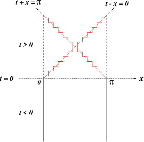
Figure 1: The solid and dashed vertical lines denote the boundaries at $x=0,\,\pi$, where the Neumann and the Dirichlet boundary conditions are imposed, respectively. The dashed vertical lines mimic the emerging naked singularities. Thunderbolts, denoted by zigzag lines, appear along the null lines, $z_{+}=\pi$ and $z_{-}=0$.

4 Summary and Discussion

We have studied quantum effects of the sudden change of the boundary conditions which mimics the occurrence of wave-singular naked singularities. To be specific, we have dealt with the massless scalar field in $(1+1)$-dimensional Minkowski spacetime with finite spatial interval. We have shown that the particle creations occur due to the sudden change of the boundary condition from the Neumann to the Dirichlet condition at $t=0$. Quantum particle creation is known to happen when the time-translation operator, or the Hamiltonian is time dependent. As we have emphasized, an operator of the spatial part of the wave equation is defined as a pair of the action $A$ and its domain of definition ${\cal D}(A)$. The sudden change of the boundary condition is nothing but the change of the domain ${\cal D}(A)$ so that in this sense the time-translation operator is time dependent. The behavior of the Bogoliubov coefficients in this model implies that the unitarity implementability breaks down, and the Fock space for $t>0$ is not equivalent to the one for $t<0$. Furthermore, having computed the vacuum expectation value of the energy-momentum tensor, we explicitly showed that, the singular null waves or the thunderbolts appear along the null lines emanating from the edges of the emerging singularities, while the energy-momentum tensor is the Casimir energy inside the future domain of dependence of the initial hypersurface.

Our result suggests that the Cauchy horizon associated with wave-singular naked singularities will be destroyed by the thunderbolts and the global hyperbolicity will be restored by the quantum effects. Thus this will be a support for quantum cosmic censorship stating that wave-regular naked singularities could appear but wave-singular ones are not admitted to emerge when quantum theoretical effects are taken into account.

Although the present analysis is restricted to the simplest case such that the boundary conditions change from the Neumann condition to the Dirichlet condition, it is possible to explicitly work out the general boundary condition case. Since $U(N)$ parameters which appear in general boundary condition characterize the hair of a wave-singular naked singularity, the calculation of the general boundary conditions case will tell us the relation between the strength of thunderbolt and a hair of the wave-singular naked singularity. A brief discussion of the general boundary condition case is given in the appendix.

In the present work we have examined only the $(1+1)$-dimensional model, for explicit demonstration. The results might be applicable even to the 4-dimensional spacetime case, following the discussion by Anderson and DeWitt [8]. The point is that the appearance of the thunderbolts is due to the sudden change of the domain ${\cal D}(A)$ of $A$ at the initial surface. The discontinuous change of the basis functions $\{f_{n}\}$ of ${\cal D}(A)$ implies a delta-function like behavior of the gradient $\nabla f_{n}$ at the initial surface. Since the energy-momentum tensor is bilinear in $\nabla f_{n}$, the square of the delta-function, like the second term of Eq. (31), are naturally expected to appear in a $4$-dimensional setup.

So far there have appeared many works on quantum effects around a Cauchy horizon, showing the divergence of the expectation value of the energy-momentum tensor along or near the horizon (See e.g., Review [16] and references therein). The particle creation occurs as a result of the spacetime dynamics just before the instant of the naked singularity formation by gravitational collapse (See e.g., Ref. [17]), but is not directly related to the nature of the singularity itself. On the other hand, in the present simple analysis, no dynamics of the spacetime metric has been considered. The appearance of the thunderbolts may be interpreted as a result of the wave scattering off at $t=0+$ by the boundary singularities. We can extend our present analysis to a gravitational collapse model in $(3+1)$-dimensions. Then as commented above, we expect a quantum effect, leading to the thunderbolt. This is a new phenomenon, because it is not merely a consequence of dynamics which creates naked singularities but directly reflects the character of the wave-singular naked singularities.

Appendix

Here we shall consider the general boundary condition case in which the boundary conditions at $x=0,\,\pi$ are given as $b\,\partial_{x}\phi=\phi$ before the incident $t=0$ but suddenly changes to $a\,\partial_{x}\phi=\phi$ after $t=0$, with $a,b$ being constants. Note that when $a,b=0$, the field satisfies the Dirichlet boundary condition and when $a,b\rightarrow\infty$, the Neumann boundary condition.

The positive frequency (in)- and (out)- mode functions are respectively given by

$$f^{(out)}_{m}(t,x) = \frac{e^{-imt}}{\sqrt{\pi m}}\frac{1}{\sqrt{1+a^{2}m^{2}}}\left(\sin mx+am\cos mx\right)\,,\quad\mbox{in $t>0$}\,,$$ (33)

$$f^{(in)}_{n}(t,x) = \frac{e^{-int}}{\sqrt{\pi n}}\frac{1}{\sqrt{1+b^{2}n^{2}}}\left(\sin nx+bn\cos nx\right)\,,\quad\mbox{in $t<0$}\,,$$ (34)

so that $b\,\partial_{x}{f^{(in)}_{n}}=f^{(in)}_{n}$ and $a\,\partial_{x}{f^{(out)}_{m}}=f^{(out)}_{m}$ at $x=0,\,\pi$. Besides these positive frequency modes, when $a$ or $b\rightarrow\infty$, there exist zero-modes. But here we do not treat the contributions from zero-modes, just for simplicity.

Then, following the same step in Section 3.2, we can find the Bogoliubov coefficients:

$$\alpha_{nn} = \frac{1+abn^{2}}{\sqrt{1+a^{2}n^{2}}\sqrt{1+b^{2}n^{2}}}\delta_{m,n}\,,$$ (35)

$$\alpha_{mn} = \frac{2}{\pi}(b-a)\frac{\sqrt{mn}}{\sqrt{1+a^{2}m^{2}}\sqrt{1+b^{2}n^{2}}}\frac{1}{m-n}\delta_{m\pm n:odd}\,,$$ (36)

$$\beta_{mn} = \frac{2}{\pi}(b-a)\frac{\sqrt{mn}}{\sqrt{1+a^{2}m^{2}}\sqrt{1+b^{2}n^{2}}}\frac{1}{m+n}\delta_{m\pm n:odd}\,.$$ (37)

From this we can immediately see that, if $ab\neq 0$, then $\sum_{n=1}^{\infty}\sum_{m=1}^{\infty}|\beta_{nm}|^{2}$ is finite, while if $ab=0\,(a\neq b)$, then it is logarithmically divergent, hence in this case the Fock space of the (in)-states and that of the (out)-states are unitarily inequivalent.

The vacuum expectation value of the energy-momentum tensor can be computed in the same way in Section 3.4. The result can be written down in terms of Lerch’s transcendent, which is rather complicated and not so illuminating for drawing the physical consequence.

References

- [1] R.M. Wald, Gravitational Collapse and Cosmic Censorship, gr-qc/9710068.
- [2] A. Ishibashi and A. Hosoya, Phys. Rev. D 60, 104028 (1999).
- [3] C.J.S. Clarke, Class. Quantum Grav. 15, 975 (1998).
- [4] J.A. Vickers and J.P. Wilson, Class. Quantum Grav. 17, 1333 (2000).
- [5] J.A. Vickers and J.P. Wilson, Generalised hyperbolicity: hypersurface singularities, gr-qc/0101018.
- [6] M. Natsuume, The Singularity Problem in String Theory, gr-qc/0108059.
- [7] S.W. Hawking and J.M. Stewart, Nucl. Phys. B400, 393 (1993).
- [8] A. Anderson and B. DeWitt, Found. Phys. 16, 91 (1986).
- [9] J. Polchinski, String Theory, Volume I, Volume II, (Cambridge University Press, Cambridge, United Kingdom 1998).
- [10] M. Reed and B. Simon, Fourier Analysis, Self-Adjointness, (Academic Press, New York, 1975).
- [11] R.M. Wald, J. Math. Phys. 21, 2802 (1980).
- [12] G.T. Horowitz and D. Marolf, Phys. Rev. D 52, 5670 (1995).
- [13] B.S. DeWitt, Phys. Rep. 19C, 295 (1975).
- [14] H. Kodama, Prog. Theor. Phys. 64, 2267 (1980).
- [15] N.D. Birrell and P.C.W. Davies, Quantum fields in curved space, (Cambridge University Press, Cambridge, 1982).
- [16] T.P. Singh, Comparing quantum black holes and naked singularities, Proceedings for the conference JGRG 10 (unpublished), gr-qc/0012087.
- [17] T. Harada, H. Iguchi, K. Nakao, T.P. Singh, T. Tanaka, and C. Vaz, Phys. Rev. D 64, 041501 (2001).