Towards the QFT on Curved Spacetime Limit of QGR.
I: A General Scheme

Abstract

In this article and the companion paper [1] we address the question of how one might obtain the semiclassical limit of ordinary matter quantum fields (QFT) propagating on curved spacetimes (CST) from full fledged Quantum General Relativity (QGR), starting from first principles. We stress that we do not claim to have a satisfactory answer to this question, rather our intention is to ignite a discussion by displaying the problems that have to be solved when carrying out such a program.

In the first paper of this series of two we propose a general scheme of logical steps that one has to take in order to arrive at such a limit. We discuss the technical and conceptual problems that arise in doing so and how they can be solved in principle. As to be expected, completely new issues arise due to the fact that QGR is a background independent theory. For instance, fundamentally the notion of a photon involves not only the Maxwell quantum field but also the metric operator – in a sense, there is no photon vacuum state but a “photon vacuum operator”! Such problems have, to the best of our knowledge, not been discussed in the literature before, we are facing squarely one aspect of the deep conceptual difference between a background dependent and a background free theory.

While in this first paper we focus on conceptual and abstract aspects, for instance the definition of (fundamental) $n-$particle states (e.g. photons), in the second paper we perform detailed calculations including, among other things, coherent state expectation values and propagation on random lattices. These calculations serve as an illustration of how far one can get with present mathematical techniques. Although they result in detailed predictions for the size of first quantum corrections such as the $\gamma$-ray burst effect, these predictions should not be taken too seriously because a) the calculations are carried out at the kinematical level only and b) while we can classify the amount of freedom in our constructions, the analysis of the physical significance of possible choices has just begun.

1 Introduction

Canonical, non-perturbative Quantum General Relativity (QGR) has by now reached the status of a serious candidate for a quantum theory of the gravitational field: First of all, the formulation of the theory is mathematically rigorous. Although there are no further inputs other than the fundamental principles of four-dimensional, Lorentzian General Relativity and quantum theory, the theory predicts that there is a built in fundamental discreteness at Planck scale distances and therefore an UV cut-off precisely due to its diffeomorphism invariance (background independence). Next, while most of the results have so far been obtained using the canonical operator language, also a path integral formulation (“spin foams”) is currently constructed. Furthermore, as a first physical application, a rigorous, microscopical derivation of the Bekenstein-Hawking entropy – area law has been established. The reader interested in all the technical details of QGR and its present status is referred to the exhaustive review article [2] and references therein, and to [3] for a less technical overview. For a comparison with other approaches to quantum gravity see [4, 5, 6].

A topic that has recently attracted much attention is to explore the regime of QGR where the quantized gravitational field behaves “almost classical”, i.e. approximately like a given classical solution to the field equations. Only if such a regime exists, one can really claim that QGR is a viable candidate theory for quantum gravity. Consequently, efforts have been made to identify so called semiclassical states in the Hilbert space of QGR, states that reproduce a given classical geometry in terms of their expectation values and in which the quantum mechanical fluctuations are small [7, 8, 9, 10, 11]. Also, it has been investigated how gravitons emerge as carriers of the gravitational interaction in the semiclassical regime of the theory [12, 13, 14]. The recent investigation of Madhavan and others [15, 16, 17, 18] on the relation between the Fock representations used in conventional quantum field theories and the one in QGR further illuminate the relation between QGR and a perturbative treatment based on gravitons.

In this and the companion paper [1] we would also like to contribute to the understanding of the semiclassical limit of QGR: We will investigate how the theory of quantum matter fields propagating in a fixed classical background geometry (QFT on CST) arises as an approximation to the full theory of QGR coupled to (quantum) matter fields. We will show in section 4 of the present work, how, upon choosing a semiclassical state, an effective QFT for the matter fields can be obtained from a more fundamental theory of QGR coupled to matter. This effective theory turns out to be very similar to standard QFT on CST, but still carries an imprint of the discreteness of the geometry in QGR as well as of the quantum fluctuations in the gravitational field.

Validating the semiclassical limit of matter coupled to QGR is not the only motivation for the present work. Since QGR is a background independent theory, the consistent coupling of matter fields requires a quantum field theoretical description of these fields that differs considerably from that used in ordinary QFT. Therefore, another aim of the present work is to gain some insights into what these differences are and how matter QFT can be formulated in a setting where also the gravitational field is quantized. As a main result of the present paper we show how a theory of matter coupled to quantum geometry can be formulated within the framework of QGR. Within this theory we identify states that can roughly be compared to the $n$-particle states occurring in ordinary QFT. Their structure is however fundamentally different as compared to that of the ordinary Fock states: Their definition also involves operators of the gravitational sector of the theory!

Similar considerations may be applied to understand the emergence of gravitons in the semiclassical limit of QGR. The situation there is however a bit more complicated since it requires the separation of the gravitational field in a background- and a graviton-part. We refer the reader to [19] where a detailed consideration will be given.

Finally, due to a better understanding of the phenomenology of quantum gravity and the experiments that could lead to its detection (see [20] for a recent review) it is an intriguing question whether it might already be possible to make predictions for observable quantum gravity effects based on QGR. In order to do so, one has to consider a coupling of the gravitational field to matter – one can not measure the gravitational field directly but only through its action on other fields. Indeed, ground-breaking work on the phenomenology of QGR has been done [21, 22, 23, 24]. In these works, corrections to the standard dispersion relations for matter fields due to QGR have been obtained. Since we are dealing with a theory for matter coupled to QGR in the present work, it is an important question whether the results of [21, 22, 23, 24] can be confirmed in the present setting. We will discuss the general aspects of this question in section 5. In the companion paper [1] we will carry out a more detailed calculation, based on the results of the present work and the semiclassical states constructed in [9, 10, 11].

The main difficulty in carrying out the program outlined up to now lies in the fact that the full dynamics of quantum gravity coupled to quantum matter is highly complicated. This would already be the case for ordinary interacting fields but is amplified in the present case due to the complicated interaction terms (the gravitational field enters in a non-polynomial way) and the difficulties in the interpretation of the resulting solutions. In the setting of QGR, the dynamics is implemented in the spirit of Dirac, by turning the Hamilton constraint of the classical theory into an operator and restricting attention to (generalized) states in its kernel. A mathematically well-defined candidate Hamiltonian constraint operator has been proposed in [25, 26, 27, 28, 29] (see also [30, 31] for another proposal based on Vasiliev invariants). This operator turns out to be very complicated and a systematic analysis of its kernel seems presently out of reach. Therefore, in our considerations, we can not start from a fully quantized dynamical theory of gravity coupled to matter. Instead, we have to treat the dynamics in some rather crude approximation and therefore our considerations will be kinematical to a large extent. To be more precise, we will not treat the the matter parts in the Hamiltonian as constraints, but as Hamiltonians generating the dynamics of the matter fields in the ordinary QFT sense. With the part in the Hamiltonian describing the self interaction of the gravitational field we will deal by using semiclassical states, which, as we will explain, annihilate this part of the Hamiltonian constraint at least approximately. Proceeding in this way certainly only amounts to establishing an approximation to the full theory: The self interaction of gravity and the back-reaction of the matter fields on the geometry are only partly reflected by using semiclassical states that approximate a classical solution to the field equations of the gravity-matter system.

What we gain is a relatively easy to interprete, fully quantized theory of gravity and matter fields. This way we have “a foot in the door” to the fascinating topic of interaction between quantum matter and quantum gravity and can start to discuss the conceptual issues arising, as well as take some steps towards the prediction of observable effects resulting from this interplay.

Let us finish this introduction with a brief description of the structure of the rest of the article: In the next section, we will discuss the main steps taken in this work in more detail before we turn to their technical implementation in the subsequent sections.

In section 3 we give a very brief introduction to the formalism of QGR, mainly to fix our notation. In more detail we display the matter Hamiltonian operators of electromagnetic, scalar and Dirac matter when coupled to general relativity.

Section 4 contains the main results of this paper, namely a proposal for how to arrive at the notion of Fock states or $n-$particle states on fluctuating quantum spacetimes, if one is to start from a fundamental quantum theory of gravity of matter.

In section 5 we discuss various methods to obtain dispersion relations for the matter fields from the full theory described in 3.

We conclude this work with a discussion of its results and possible directions for future research in section 6.

In an appendix, we treat the toy model of two coupled Harmonic oscillators to give an example of how the results are affected when one uses kinematical coherent states instead of coherent states in the dynamical Hilbert space of the theory.

As already said, in the present paper we focus on describing the general scheme, detailed calculations will appear in the companion paper [1].

2 A General Scheme

In this section we want to discuss the issues related to the QFT on CST Limit of QGR and describe the steps taken in the present work in more detail.

The first step that we will take is the kinematical quantization of the matter and the gravitational field on a Hilbert space $\mathcal{H}^{\text{kin}}$. We will be guided by the fundamental principles of QGR which have to be obeyed: The quantum theory should be formulated in a background free and diffeomorphism covariant fashion. If the matter field is a gauge field with compact gauge group, we can quantize it with exactly the same methods that are used in QGR for the gravitational field. This way, we obtain a neat unified description of gravity and the other gauge fields. Also for fermions or scalar fields, a representation should be used that is background independent. This rules out the usual Fock representation. New representations for fermionic, Higgs and scalar fields in keeping with the principles of QGR were proposed in [25] and we will use them for our purpose.

The quantization of the Hamiltonian of the coupled system is a rather nontrivial task, due to its complicated non-polynomial dependence on the basic variables of the theory. Nevertheless, a scheme for the quantization for densities of weight one has been proposed in [28, 27] which leads to well-defined candidate operators. The resulting operators are quite complicated but perfectly well defined and lead to reasonable results in a symmetry reduced context [32, 33]. Another very encouraging aspect of the scheme is that it works precisely due to the density one character of the classical quantities, which is dictated by background independence, and not only despite of it. In [1] and the present paper we will proceed along the lines given in [28, 27] and obtain Hamiltonian constraint operators for electromagnetic, scalar, and fermionic fields coupled to gravity.

As a next step we have to deal with the constraints of the theory: A Gauß constraint for Gravity and for every matter gauge field, the spatial diffeomorphism constraint of gravity, and, finally and most importantly, the Hamilton constraint of the coupled gravity-matter system.

The implementation of the diffeomorphism constraint has been accomplished in [34]. Still, there is a difficulty related to the spatial diffeomorphism constraint for pure gravity: No spatially diffeomorphism invariant quantum observables (apart from the total volume of the space-like hypersurface $\Sigma$, in case it is finite) have been constructed so far. This is due to the fact that such observables are given by integrals over $\Sigma$ of scalar densities of weight one built from the spatial curvature tensor and its spatial covariant derivatives which are highly non-polynomial functions. This problem gets alleviated when matter is coupled to the gravitational field. For instance, the matter can serve to define submanifolds or regions of $\Sigma$ in a diffeomorphism covariant way. Diffeomorphism invariant observables can then be obtained by integrating the gravitational fields over these submanifolds or regions [35, 36]. Indeed we will see that this also applies to the Hamiltonian for gravity coupled matter: The corresponding operator constructed in the next section will be diffeomorphism invariant. This is important for the following reason: Since the diffeomorphisms of $\Sigma$ are implemented unitarily on $\mathcal{H}_{\text{kin}}$, the expectation value and fluctuations of a diffeomorphism invariant operator do not differ from its expectation value and fluctuations in the state that results from projecting the original one to the diffeomorphism invariant Hilbert space (via group averaging) [34] provided the operator satisfies certain technical conditions (it has to leave cylindrical subspaces of the Hilbert space separately invariant). Therefore as long as we work with diffeomorphism invariant operators on $\mathcal{H}_{\text{kin}}$ we do not have to bother too much about implementing the diffeomorphism constraint. Similar remarks concern the Gauß constraints, so we will also not be concerned with their implementation in what follows.

We now turn to the implementation of the Hamilton constraint. Even for pure gravity, this is a very difficult topic. Though solutions have been found [29, 26], they are notoriously hard to interpret due to the lack of Dirac observables invariant under the motions generated by the Hamiltonian constraint (even in the presence of matter) and a thorough understanding of the “problem of time”. The problem of finding solutions to the Hamilton constraint for gravity coupled to matter has not been treated before although the method of [29] can in principle be applied as well.

Since one of our goals is to explore the semiclassical limit of QGR coupled to matter, the task presented to us is even harder: Not only do we have to find some solutions to the Hamilton constraint, but we are interested in specific solutions in which the gravitational field is in a state close to some given classical geometry.

As already explained in the introduction, in the light of these difficulties, we propose to proceed along slightly different lines. To give an idea what we are aiming at, imagine we ought to compute corrections to the interaction of some quantum system (an atom, say) with an electromagnetic field, which are due to the quantum nature of the electromagnetic field. Ultimately this is a problem in quantum electrodynamics and therefore certainly not solvable in full generality. What can be done? For the free Maxwell field, there is a family of states describing configurations of the quantum field close to classical ones, the coherent states: Expectation values for field operators yield the classical values and the quantum mechanical uncertainties are minimal in a specific sense. Such states could be used to model the classical electromagnetic field. Certainly these coherent states are no viable states for the full quantum electrodynamics treatment in any sense. They do not know anything about the dynamics of the full theory. The key point now is that though being in some sense “kinematical”, the coherent states for the Maxwell field are nevertheless a very good starting point to compute approximate quantum corrections as testified by the computations in the framework of quantum optics [37]. Certainly this analogy is not complete in that QED is equipped with a true Hamiltonian (rather than just a Hamiltonian constraint) but it shows nevertheless that sometimes kinematical states lead to rather good approximations.

In the present work we will proceed in the same spirit: We will not seek states which are solutions to the constraint and approximately correspond to some classical geometry, but rather start by considering kinematical semiclassical states.

Consequently, we treat the Hamiltonians of the matter fields not as pieces of the Hamiltonian constraint but rather as observables. In particular, there will be no lapse function, these Hamiltonian operators are simply different operators (from the Hamiltonian constraint operator). Although we will follow essentially the steps performed in [27], the fact that we are dealing with different operators allows us to change the quantization procedure slightly, for instance, the Hamiltonian operators leave the cylindrical subspaces of ${\cal H}_{kin}$ separately invariant.

It is hard to judge the validity of this approach as compared to the desirable full fledged solution of the Hamilton constraint. To shed some light on this issue, in an appendix we consider a simple quantum mechanical model system. For this system we can show that the expectation values of Dirac observables in coherent states states on the kinematical level numerically differ from the results of a treatment using dynamical coherent states, the differences are tiny, however, as long as the energy of the system is macroscopic.

Another issue raised by the treatment outlined above is that much depends on the choice of the state that is employed to play the role of the semiclassical state. We will defer a discussion of this fascinating topic to the companion paper [1] and only make some brief remarks here:

All candidate semiclassical states proposed so far are graph based states, i.e. cylindrical functions in $\mathcal{H}_{\text{kin}}$. Consequently, this is assumed to be the case in the present work. The picture might however change substantially if ideas such as the averaging over infinitely many graph based states advocated in [8] could be employed. For some more discussion on this point we refer to [1, 38].

Having adopted the above viewpoint on the Hamilton constraint, we can construct approximate $n-$particle Fock states propagating on fluctuating quantum spacetimes as follows: Denote by ${\cal M}$ the gravitational phase space of initial data on the hypersurface $\Sigma$ of the differentiable manifold $M={\mathchoice{\hbox{\hbox to0.0pt{\kern 2.9444pt\vrule height=6.14993pt\hss}\hbox{$\displaystyle\rm R$}}}{\hbox{\hbox to0.0pt{\kern 2.9444pt\vrule height=6.14993pt\hss}\hbox{$\textstyle\rm R$}}}{\hbox{\hbox to0.0pt{\kern 2.06108pt\vrule height=4.30496pt\hss}\hbox{$\scriptstyle\rm R$}}}{\hbox{\hbox to0.0pt{\kern 1.4722pt\vrule height=3.07497pt\hss}\hbox{$\scriptscriptstyle\rm R$}}}}\times\Sigma$. Let $m\in{\cal M}$ be initial data for some background spacetime. An ordinary $n-$ particle state is an excitation of a vacuum state $\Omega^{\text{Fock}}_{\text{matter}}(m)$ in a usual Fock space ${\cal H}^{\text{Fock}}_{\text{matter}}(m)$ which is of a completely different type than the background independent Hilbert space ${\cal H}^{\text{kin}}_{\text{matter}}$. The construction of that vacuum state (and the entire Fock space) makes heavy use of the background metric in question, here indicated by the explicit dependence of the state on the point $m$ in the gravitational phase space. This dependence slips in because the state $\Omega^{\text{Fock}}_{\text{matter}}(m)$ is usually chosen as the ground state of some Hamiltonian operator $\hat{H}_{\text{matter}}(m)$ on the background spacetime in question. We now see what will heuristically happen when we start switching on the gravitational fluctuations as well: The dependence of $\Omega^{\text{Fock}}_{\text{matter}}(m)$ on $m$ has to become operator valued! In other words, the vacuum state function $m\mapsto\Omega_{\text{matter}}(m)$ becomes a vacuum operator $\hat{\Omega}:=\Omega_{\text{matter}}(\hat{m})$, that is, a function of the matter degrees of freedom with values in ${\cal L}({\cal H}^{\text{kin}}_{\text{grav}})\otimes{\cal H}^{\text{kin}}_{\text{matter}}$ where ${\cal H}^{\text{kin}}_{\text{matter}}$ is now necessarily a background independent matter Hilbert space (which we have chosen to be the one currently in use in QGR) and ${\cal L}({\cal H}^{\text{kin}}_{\text{grav}})$ denotes the space of linear operators on a background independent geometry Hilbert space. We see that the whole concept of an $n-$particle state becomes a very different one in the background independent context! Of course, we do not want a vacuum operator but a vacuum state on the full Hilbert space ${\cal H}^{\text{kin}}$ so that one will apply the vacuum operator to a state $\psi_{\text{grav}}(m)\in{\cal H}^{\text{kin}}_{\text{grav}}$, that is, $\Omega(m)=\hat{\Omega}\psi_{m}$.

We conclude that a fundamental $n-$particle state of some matter type corresponding to an ordinary $n-$particle state of the same matter type propagating on some background spacetime described by the point $m$ in the gravitational phase space will be a complicated linear combination of states of the form $\psi_{\text{grav}}(m)\otimes\psi_{\text{matter}}\in{\cal H}^{\text{kin}}_{\text{grav}}\otimes{\cal H}^{\text{kin}}_{\text{matter}}\;.$ How should this state be obtained from first principles? We propose the following strategy: Consider the full gravity coupled Hamiltonian operator $\hat{H}$ and construct a annihilation operator from it, which is now an operator on the full Hilbert space ${\cal H}^{\text{kin}}$ and whose partial classical limit at the point $m$ of the gravitational phase space with respect to the gravitational degrees of freedom mirrors the usual Fock space annihilation operator on the background spacetime described by $m$.

This is what one should do. Now recall that the construction of Fock space annihilation operators on a given background involves, for instance, the construction of fractional powers of the Laplacian operator on that background metric which is an operator in the one-particle (or first quantized matter) Hilbert space. Thus, our fundamental annihilation operator will involve a quantization of these Laplacian operators which therefore become an operator on the tensor product of the one particle Hilbert space and the gravitational Hilbert space ${\cal H}^{\text{kin}}_{\text{grav}}$. While we are able to actually construct these operators in the present paper, as one can imagine, the formulas that we obtain are too complicated in order to do practical computations with present mathematical technology because fractional powers of the Laplacian are defined via its spectral resolution which is difficult to find.

As an approximation to this exact computation we therefore propose to first compute the expectation value of the Laplacian operator in a gravitational coherent state and then to take its fractional powers. Now, precisely because we are using coherent states, this approximation will coincide with the exact calculation to zeroth order in $\hbar$ while for higher orders we presently do not know how significantly results are changed. The details of these statements will be presented in section 4.

The last step in the program is then to obtain, in principle testable, predictions from the theory obtained so far. For instance, we are interested in states of the form $\psi_{\text{grav}}(m)\otimes\psi_{\text{matter}}\in{\cal H}^{\text{kin}}_{\text{grav}}\otimes{\cal H}^{\text{kin}}_{\text{matter}}$ and wish then to construct an effective matter Hamiltonian operator as a quadratic form through the formula

$$<\psi_{\text{matter}},\hat{H}^{\text{eff}}_{\text{matter}}(m)\psi^{\prime}_{\text{matter}}>_{{\cal H}^{\text{kin}}_{\text{matter}}}:=<\psi_{\text{grav}}(m)\otimes\psi_{\text{matter}},\hat{H}\psi_{\text{grav}}(m)\otimes\psi^{\prime}_{\text{matter}}>_{{\cal H}^{\text{kin}}_{\text{grav}}\otimes{\cal H}^{\text{kin}}_{\text{matter}}}$$

The operator $\hat{H}^{\text{eff}}_{\text{matter}}(m)$ already contains information about the quantum fluctuations of geometry. The quantum fluctuations of matter are certainly much larger than those of geometry in the energy range of interest to us, however, as we are interested in Poincaré invariance violating effects, which are excluded by definition in ordinary QFT on Minkowski space, in order to study those we can neglect the quantum effects of matter as a first approximation (that is, we are dealing with free field theories except for the coupling to the gravitational field). Therefore, we take the classical limit of $\hat{H}^{\text{eff}}_{\text{matter}}(m)$ and study the wave like solutions of the matter dynamics it generates. One can also take the point of view that this procedure corresponds to the first quantization of matter on a fluctuating spacetime. Second quantization will then be studied later on when we discuss $n-$particle states.

Adopting this viewpoint, as soon as a semiclassical state for the gravity sector is chosen, translation and rotation symmetry is heavily broken on short scales due to the discreteness of the underlying graph. The theory describes fields propagating on random lattices, bearing a remarkable similarity to models considered in lattice gauge theory [39, 40, 41]. Due to the lack of symmetry on short scales, notions such as plane waves and hence dispersion relations can at best be defined in some large scale or low energy limit. We will show that the problem of treating these limits is by no means trivial and requires careful physical considerations. It is closely related to the condensed matter physics problem of computing macroscopic parameters of an amorphous (i.e. locally anisotropic and inhomogeneous) solid from the parameters of its microscopic structure.

To get a feeling for the problem, we will sketch a one dimensional model system for which we are able to find exact solutions. We will then turn to general fields on random lattices and describe a procedure to obtain dispersion relations valid in the long wavelength regime.

This concludes our explanatory exposition. We will now proceed to the details.

3 Review of Quantum Kinematics of QGR

In QGR the manifold underlying spacetime is taken to be diffeomorphic with $M=\mathbb{R}\times\Sigma$ where $\Sigma$ represents a 3d manifold of arbitrary topology. We will now summarize the essential aspects of the kinematical framework of [25] for matter fields coupled to quantum gravity. We also introduce the Hamiltonians that we will be deriving dispersion relations for.

Gravity and Gauge Theory Sector

The canonical pair consists of a $G$ connection $A^{i}_{a}(x)$ for a compact gauge group $G$ and a Lie$(G)$ valued densitized vector field $E_{i}^{a}(x)$ on $\Sigma$. Here we can treat all four interactions on equal footing. For the gravitational sector we have $G=SU(2)$ and the relation of the canonical pair to the classical ADM variables $q_{ab}$, $K_{ab}$ is

$$\det(q)q^{ab}=\iota E^{a}_{i}E^{bi},\qquad A^{i}_{a}=\Gamma^{i}_{a}-\frac{\iota}{\sqrt{\det(q)}}K_{ab}E^{bi},$$

where $\Gamma$ is the spin connection corresponding to the triad $E$, and $\iota$ is the Barbero-Immirzi parameter which can in principle take any nonzero value in $\mathbb{C}$ [42, 43]. We will choose $\iota=1$ in what follows. As for units, we choose $[A]=\text{meter}^{-1}$. As a consequence, $E$ will be dimensionless for gravity and has dimension cm^-2 for Yang-Mills theories.

In the following we will have frequent opportunity to use the notion of graphs embedded in $\Sigma$:

Definition 3.1.

By an edge $e$ in $\Sigma$ we shall mean an equivalence class of analytic maps $[0,1]\longrightarrow\Sigma$, where two such maps are equivalent if they differ by an orientation preserving reparametrization.
A graph in $\Sigma$ is defined to be a set of edges such that two distinct ones intersect at most in their endpoints.

There is some notation in connection to graphs that we will use frequently:
The endpoints of an edge $e$ will be called vertices and denoted by $b(e)$ (the beginning point of $e$), $f(e)$ (the final point of $e$).
The set of edges of a graph $\gamma$ will be denoted by $E(\gamma)$, the set of vertices of its edges by $V(\gamma)$.
Given a graph $\gamma$, we will denote the edges of $\gamma$ having $v$ as vertex by $E(\gamma,v)$ or $E(v)$ if it is clear which graph we are referring to.
Given a graph $\gamma$, a vertex $v\in V(\gamma)$ and an edge $e\in E(v)$ we define

$$\sigma(v,e)=\begin{cases}+1&\text{ if }b(e)=v\\ -1&\text{ if }f(e)=v\\ 0&\text{ if $e$ is not adjacent to $v$}\\ \end{cases}.$$

Thus $e^{\sigma(v,e)}$ is always outgoing with respect to $v$.

Being a one-form, $A$ can be integrated naturally (that is, without recurse to background structure) along piecewise analytic curves $e$ in $\Sigma$, to form holonomies

$$h_{e}[A]=\operatorname{\mathcal{P}}\exp\left[i\int_{e}A\right]\qquad\in G.$$

It is convenient to consider a class of functionals of the connection $A$ a bit more general:

Definition 3.2.

A functional $f[A]$ of the connection is called cylindrical with respect to a piecewise analytical graph $\gamma$ if there is a function

$$f:G^{\left\lvert E(\gamma)\right\rvert}\longrightarrow\mathbb{C},$$

such that

$$f[A]=f(h_{e_{1}}[A],h_{e_{2}}[A],\ldots),\qquad\qquad e_{1},e_{2},\ldots\in E(\gamma).$$ (3.1)

The density weight of $E$ on the other hand is such that, using an additional real internal vector field $f^{i}$ it can be naturally integrated over surfaces $S$ to form a quantity

$$E_{S,f}=\int_{S}f^{i}\;(*E)_{i}$$

analogous to the electric flux through $S$.

In the connection representation of diffeomorphism invariant gauge field theory, quantization of the Poisson algebra generated by the classical functions $\operatorname{Cyl}$ and the vector space space of electric fluxes $\operatorname{\mathcal{E}}$ is achieved on the Ashtekar-Lewandowski Hilbert space

$$\mathcal{H}_{0}=L^{2}(\overline{\mathcal{A}},d\mu_{0}).$$

It is based on the compact Hausdorff space $\overline{\mathcal{A}}$ of generalized connections which is a suitable enlargement of the space of smooth connections $\mathcal{A}$ and the uniform measure $\mu_{0}$.

The classical Yang-Mills Hamiltonian (coupled to gravity) reads

$$H_{YM}=\frac{1}{2Q_{YM}}\int_{\Sigma}d^{3}x\frac{q_{ab}}{\sqrt{\det(q)}}[E^{a}_{I}E^{b}_{J}+B^{a}_{I}B^{b}_{J}]\delta^{IJ}.$$ (3.2)

Here $Q_{YM}$ is the Yang-Mills coupling constant, $E^{a}_{I}$ is the Yang-Mills electric field, $B^{a}_{I}=\epsilon^{abc}F_{bc}^{I}$ the magnetic field associated with the Yang-Mills curvature $F_{ab}^{I}$.

We now quantize this operator along the lines of [27], actually only for Maxwell Theory since in this paper we are interested only in free theories when taking the metric as a background field. Here we take advantage of the fact that $\hat{H}_{YM}$ is an operator of its own although, of course, the integrand of (3.2) is a piece of the classical Hamiltonian constraint of geometry and matter. Accordingly we may exploit the quantization ambiguity concerning the loop attachment in [27] as follows: We define the operator $\hat{H}_{YM}$ consistently on the combined spin-network basis of matter and geometry introduced in [25] and use the following notion.

Definition 3.3.

Let a graph $\gamma$, a vertex $v\in V(\gamma)$ and two different edges $e,e^{\prime}\in E(\gamma)$ incident at $v$ be given. By a minimal loop based at $v$ we mean a loop $\beta(\gamma,v,e,e^{\prime})$ in $\gamma$ which

• starts at $v$ along $e$ and ends at $v$ along $e^{\prime}$,

• does not self-overlap,

• the number of edges used by $\beta$ except $e,e^{\prime}$ cannot be reduced without breaking the loop into pieces.

Notice that given $\gamma,v,e,e^{\prime}$ a minimal loop does not need to be unique! Denote by $S(\gamma,v,e,e^{\prime})$ the set of minimal loops corresponding to the data indicated and by $L(\gamma,v,e,e^{\prime})$ their number. Notice also that the notion of a minimal loop does not make any reference to a background metric, it is an object that belongs to the field of algebraic graph theory [44, 45, 46].

Here we see the first difference as compared to the loop choice in [27]: A minimal loop is always contained in the graph that we are dealing with. The second difference that we will introduce in contrast to [27] is that there we used functions of holonomies of the type $H_{\beta}-H_{\beta}^{-1}$ in order to express the Yang-Mills magnetic field in terms of holonomies. However, as correctly pointed out in [47], the regularization ambiguity allows more general functions, the only criterion is that the final operator is gauge invariant and that the function should vanish at trivial holonomy. Our preliminary proposal for the Maxwell Hamiltonian operator, projected to spin-network states over graphs $\gamma$ is then

$$\hat{H}_{M,\gamma} = -\frac{\alpha m_{P}}{2\ell_{P}^{3}}\sum_{v\in V(\gamma)}\sum_{v\in e\cap e^{\prime}}[\frac{3}{N(\gamma,v)}]^{2}\hat{Q}^{j}_{e}(v,\frac{1}{2})\hat{Q}^{j}_{e^{\prime}}(v,\frac{1}{2})\times$$ (3.3)

$$\times \{-Y_{e}Y_{e^{\prime}}+\frac{1}{P(\gamma,v,e)P(\gamma,v,e^{\prime})\alpha^{2}}[\sum_{v\in e_{1}\cap e_{2};e_{1},e_{2}\perp e}\frac{1}{L(\gamma,v,e_{1},e_{2})}\sum_{\beta\in S(v,\gamma,e_{1},e_{2})}\frac{\ln(H_{\beta})}{i}]\times$$

$$\times[\sum_{v\in e^{\prime}_{1}\cap e^{\prime}_{2};e^{\prime}_{1},e^{\prime}_{2}\perp e^{\prime}}\frac{1}{L(\gamma,v,e^{\prime}_{1},e^{\prime}_{2})}\sum_{\beta\in S(v,\gamma,e^{\prime}_{1},e^{\prime}_{2})}\frac{\ln(H_{\beta})}{i}]\},$$

where for a vertex $v$, a real positive number $r$ and an edge $e$ starting at it we have defined the basic operator

$$\hat{Q}^{j}_{e}(v,r):=\frac{1}{4r}\mbox{tr}(\tau_{j}h_{e}[h_{e}^{-1},(\hat{V}_{v})^{r}]),$$ (3.4)

with $\hat{V}_{v}$ the volume operator [48, 49] over an arbitrarily small open region containing $v$. We are using a basis of $su(2)$ with $\mbox{tr}(\tau_{j}\tau_{k})=-2\delta_{jk}$. Here $\alpha=\hbar Q_{M}$ is the Feinstruktur constant and $m_{P},\ell_{P}$ are the Planck mass and length respectively. We have adapted the coefficients of [27] to the case of $G=U(1)$ and we have distinguished the Maxwell holonomy $H$ from the gravitational holonomy $h$. $Y_{e}$ is the right invariant vector field on $U(1)$ with respect to the degree of freedom $H_{e}$. The notation $e\perp e^{\prime}$ means that $e\not=e^{\prime},e\cap e^{\prime}=v\not=\emptyset$ and that the tangents of $e,e^{\prime}$ at $v$ are linearly independent. The number $P(\gamma,v,e)$ is the number of pairs of edges $e_{1},e_{2}$ with $v\in e_{1}\cap e_{2};e_{1},e_{2}\perp e$ and $N(\gamma,v)$ denotes the valence of the vertex $v$. For each vertex $v$ the edges incident at $v$ are supposed to be outgoing from $v$, otherwise replace $e$ by $e^{\sigma(v,e)}$ everywhere in (3.3). The branch of the logarithm involved in (3.3) is defined by $\ln(1)=0$. The logarithm is convenient in order to define photon states later on but any other choice will do as well, just giving rise to more quantum corrections.

The manifestly gauge invariant and spatially diffeomorphism invariant Hamiltonian (3.3) is preliminary because we may want to order it differently later on. Notice that it does not have the correct classical limit on an arbitrary graph, the graph has to be sufficiently fine in order to reach it! We will show that it defines a positive definite, essentially self-adjoint operator on ${\cal H}_{\text{kin}}$.

Lemma 3.1.

For any positive real $r$ the operator $i\widehat{Q}^{j}_{e}(v,r)$ on $\mathcal{H}_{0}$ defined by (3.4) is essentially self-adjoint with core given by the core of $\widehat{V}_{v}$.

Proof.

Since $(h_{e})_{AB}$ is a bounded operator it suffices to show that $i\widehat{Q}^{j}_{e}(v,r)$ is symmetric with dense domain the core of $\widehat{V}_{v}$.
Using that $[(h_{e})_{AB}]^{\dagger}=(h_{e}^{-1})_{BA}$ and $\overline{(\tau_{J})_{AB}}=-(\tau_{J})_{BA}$ we find

$$4r[i\;\widehat{Q}^{j}_{e}(v,r)]^{\dagger} =i\overline{(\tau_{j})_{AB}}\left[\left((h_{e}^{-1})_{CA}\right)^{\dagger},V_{v}^{r}\right]\left((h_{e})_{BC}\right)^{\dagger}=-i(\tau_{j})_{BA}\left[\left((h_{e})_{AC}\right),V_{v}^{r}\right]\left((h_{e}^{-1})_{CB}\right)$$

$$=-i\operatorname{Tr}\left(\tau_{j}\left[\left((h_{e})\right),\widehat{V}_{v}^{r}\right]h_{e}\right)=-i\operatorname{Tr}\left(\tau_{J}h_{e}\widehat{V}_{v}^{r}h_{e}^{-1}\right)$$

$$=i\operatorname{Tr}\left(\tau_{j}h_{e}\left[h_{e}^{-1},V_{v}^{r}\right]\right)=4r[i\widehat{Q}^{j}_{e}(v,r)]$$

because $\operatorname{Tr}(\tau_{j})\widehat{V}_{v}=0$. ∎

Scalar and Higgs Fields

We will consider only Lie$(G)$ valued Higgs fields $\phi^{i}$ with canonically conjugate momentum $\pi_{i}$. In particular, a neutral scalar field $\phi$ is Lie$(U(1))$ valued and transforms in the trivial adjoint representation. We will take $\phi_{i}$ to be dimensionless, then $\pi_{i}\propto\dot{\pi}^{i}$ has dimension cm^-1.

The background independent Hilbert space of [25] is based on the quantities

$$U(x):=e^{\phi^{i}(x)\tau_{i}}\mbox{ and }\pi_{R,f}=\int_{R}d^{3}xf^{i}\pi_{i},$$ (3.5)

where $U(x)$ is referred to as point holonomy, $\tau_{j}$ is a basis of Lie$(G)$ and the second quantity is diffeomorphism covariant since $\pi_{i}$ is a scalar density. One can then quantize the Poisson algebra generated by these objects on a Hilbert space $L_{2}(\overline{{\cal U}},d\mu_{U})$ where $\overline{{\cal U}}$ is a distributional extension of the space $\cal U$ of smooth point holonomies and $d\mu_{U}$ is an associated uniform measure. This Hilbert space is very similar in spirit to the one for gauge theories displayed in (3). A dense subspace of functions in this Hilbert space consists of the cylindrical functions. Here a function is cylindrical over a graph $\gamma$, if it depends only on the point holonomies $U(v),\;v\in V(\gamma)$. That the point holonomies are restricted to the vertices of a graph is dictated by gauge invariance (for neutral scalar fields there is clearly no such argument but given a function depending on a finite number of point holonomies we can always trivially extend it to depend trivially on gravitational holonomies over a graph with the arguments of the point holonomies as vertices).

In this paper we are only interested in neutral Klein-Gordon fields without interaction potential. The unitary operator $\hat{U}(x)$ acts by multiplication while the momentum operator is densely defined by

$$\hat{\pi}_{R}f_{\gamma}=i\hbar Q_{KG}\sum_{v\in V(\gamma)\cap R}Y_{v}f_{\gamma},$$

where $Y_{v}$ denotes the right invariant vector field on $U(1)$ with respect to the degree of freedom $U(v)$ and $Q_{KG}$ is the Klein Gordon coupling constant which is such that $\hbar Q_{KG}$ has dimension cm².

The classical Klein Gordon Hamiltonian coupled to geometry is given by

$$H_{KG}=\frac{1}{2Q_{KG}}\int_{\Sigma}d^{3}x[\frac{\pi^{2}}{\sqrt{\det(q)}}+\sqrt{\det(q)}[q^{ab}\phi_{,a}\phi_{,b}+K^{2}\phi^{2}]],$$ (3.6)

where $K^{-1}$ is the Compton wave length of the Klein Gordon field. To quantize (3.6) we again copy the procedure of [27] and define it on combined matter – geometry spin-network states with the following modifications: 1) no new Higgs vertices on edges of the graph are introduced and 2) we replace the function $[U(x)-1]/i$ that substitutes $\phi(x)$ by something else in accordance to what we have said for gauge fields already. We then propose the preliminary version of the Klein Gordon Hamiltonian operator, projected to spin-network states over graphs $\gamma$ by

$$\hat{H}_{KG,\gamma} = -\frac{\hbar Q_{KG}}{2\ell_{P}^{11}}m_{p}\sum_{v\in V(\gamma)}Y_{v}^{2}\times$$ (3.7)

$$\times [\frac{1}{T(\gamma,v)}\sum_{v\in e_{1}\cap e_{2}\cap e_{3};e_{1}\perp e_{2}\perp e_{3}}\frac{1}{3!}\epsilon_{ijk}\epsilon^{IJK}\hat{Q}^{i}_{e_{I}}(v,\frac{1}{2})\hat{Q}^{j}_{e_{J}}(v,\frac{1}{2})\hat{Q}^{k}_{e_{K}}(v,\frac{1}{2})]^{\dagger}\times$$

$$\times[\frac{1}{T(\gamma,v)}\sum_{v\in e^{\prime}_{1}\cap e^{\prime}_{2}\cap e^{\prime}_{3};e^{\prime}_{1}\perp e^{\prime}_{2}\perp e^{\prime}_{3}}\frac{1}{3!}\epsilon_{lmn}\epsilon^{KLM}\hat{Q}^{l}_{e_{L}}(v,\frac{1}{2})\hat{Q}^{m}_{e_{M}}(v,\frac{1}{2})\hat{Q}^{n}_{e_{N}}(v,\frac{1}{2})]$$

$$+ \frac{1}{2\hbar Q_{KG}\ell_{P}^{7}}m_{p}\sum_{v\in V(\gamma)}\times$$

$$\times [\frac{1}{2T(\gamma,v)}\sum_{v\in e_{1}\cap e_{2}\cap e_{3};e_{1}\perp e_{2}\perp e_{3}}\epsilon^{IJK}\epsilon_{jkl}\frac{[\ln(U(f(e_{I}))-\ln(U(b(e_{I}))]}{i}\hat{Q}^{k}_{e_{J}}(v,\frac{3}{4})\hat{Q}^{l}_{e_{K}}(v,\frac{3}{4})]^{\dagger}\times$$

$$\times[\frac{1}{2T(\gamma,v)}\sum_{v\in e^{\prime}_{1}\cap e^{\prime}_{2}\cap e^{\prime}_{3};e^{\prime}_{1}\perp e^{\prime}_{2}\perp e^{\prime}_{3}}\epsilon^{LMN}\epsilon_{jmn}\frac{[\ln(U(f(e_{L}))-\ln(U(b(e_{L}))]}{i}\hat{Q}^{m}_{e_{M}}(v,\frac{3}{4})\hat{Q}^{n}_{e_{N}}(v,\frac{3}{4})]$$

$$+ \frac{(K\ell_{P})^{2}}{2\ell_{P}\hbar Q_{KG}}m_{p}\sum_{v\in V(\gamma)}[\frac{\ln(U(v)}{i}]^{\dagger}[\frac{\ln(U(v)}{i}]\hat{V}_{v},$$

where $T(\gamma,v)$ is the number of triples of edges incident at $v$ with linearly independent tangents there and $b(e)$ and $f(e)$ respectively denote starting point and end point of an edge. The operator (3.7) is again manifestly gauge and diffeomorphism invariant. Notice that $\hbar Q_{KG}/\ell_{P}^{2}$ is dimensionless while $\hat{V}_{v}$ has dimension cm³ so that all terms have mass dimension. We already have ordered terms in (3.7) in a manifestly positive way and the branch of the logarithm used corresponds to the fundamental domain of  $\textstyle\rm C$ again, i.e. $\ln(z/|z|)\in(-\pi,\pi]$.

Fermion Fields

Since the canonical, non-perturbative quantization of the Einstein-Dirac theory in four spacetime dimensions using real valued connections is maybe less familiar to the reader we review the essential aspects from [25] in slightly more detail. The classical Hamiltonian reads (we neglect coupling to the Maxwell field in this paper since we want to isolate effects of quantum gravity on the propagation of free fields, see [25, 27] for the coupling to non-gravitational forces)

$$H=\hbar\int_{\Sigma}d^{3}x\{\frac{E^{a}_{j}}{2}[{\cal D}_{a}J_{j}+i(\bar{\psi}^{T}\sigma_{j}{\cal D}_{a}\psi-\bar{\eta}^{T}\sigma_{j}{\cal D}_{a}\eta-c.c.)-K_{a}^{j}(\bar{\psi}^{T}\psi-\bar{\eta}^{T}\eta)]+iK_{0}\sqrt{\det(q)}(\bar{\psi}^{T}\eta-\bar{\eta}^{T}\psi)\}$$ (3.8)

where $K_{0}$ is the rest frame wave number, $\sigma_{j}$ are the Pauli matrices, $J_{j}:=\bar{\psi}^{T}\sigma_{j}\psi+\bar{\eta}^{T}\sigma_{j}\eta$ is the fermion current, $\psi=(\psi^{A})$ and $\eta=(\eta_{A^{\prime}})$ respectively denote the left – and right handed components of the Dirac spinor $\Psi=(\psi,\eta)^{T}$, $\bar{\psi}$ denotes the involution on Graßmann variables and the complex conjugation $c.c.$ is meant in this sense. The spinors $\psi,\eta$ transform as scalars under diffeomorphisms and as left and right handed spinors under $SL(2,{\mathchoice{\hbox{\hbox to0.0pt{\kern 2.88884pt\vrule height=6.14993pt\hss}\hbox{$\displaystyle\rm C$}}}{\hbox{\hbox to0.0pt{\kern 2.88884pt\vrule height=6.14993pt\hss}\hbox{$\textstyle\rm C$}}}{\hbox{\hbox to0.0pt{\kern 2.02219pt\vrule height=4.30496pt\hss}\hbox{$\scriptstyle\rm C$}}}{\hbox{\hbox to0.0pt{\kern 1.44441pt\vrule height=3.07497pt\hss}\hbox{$\scriptscriptstyle\rm C$}}}})$. In particular, ${\cal D}_{a}\psi=\partial_{a}\psi+\frac{1}{2}A_{a}^{j}\tau_{j}\psi,{\cal D}_{a}\eta=\partial_{a}\eta+\frac{1}{2}A_{a}^{j}\tau_{j}\eta$ where $\tau_{j}=-i\sigma_{j}$. Our convention for the Minkowski space Dirac matrices is $\gamma^{0}=-i\sigma_{2}\otimes 1_{2},\;\gamma^{j}=\sigma_{1}\otimes\sigma_{j}$ appropriate for signature $(-,+,+,+)$. The dimension of our spinor fields is cm^-3/2 so that (3.8) has indeed dimension of energy. Notice the explicit appearance of the field $K_{a}^{j}=A_{a}^{j}-\Gamma_{a}^{j}$.

A peculiarity of spinor fields is that they are their own canonical conjugates. Consider the half-densities

$$\xi:=\sqrt[4]{\det(q)}\psi,\;\;\rho:=\sqrt[4]{\det(q)}\eta,$$ (3.9)

then the canonical anti-brackets are given by

$$\{\xi_{A}(x),\bar{\rho}_{B}(y)\}_{+}=\frac{\delta_{AB}\delta(x,y)}{i\hbar},\;\;\{\rho_{A}(x),\bar{\rho}_{B}(y)\}_{+}=\frac{\delta_{AB}\delta(x,y)}{i\hbar},$$ (3.10)

while all other anti-brackets vanish. That (3.9) mixes gravitational and spinor degrees of freedom is absolutely crucial: without this peculiar mixture it would not be $A_{a}^{j}$ that is canonically conjugate to $E^{a}_{j}/\kappa$ but rather $A_{a}^{j}+i\ell_{p}^{2}e_{a}^{j}(\bar{\psi}^{T}\psi+\bar{\eta}^{T}\eta)$ which is now complex valued and this would destroy the Ashtekar Lewandowski Hilbert space ${\cal H}_{0}$ since connections would become complex valued.

Clearly, we obtain the Einstein-Weyl Hamiltonian by setting either $\xi$ or $\rho$ to zero. Likewise we can treat the case of several fermion species by adding appropriate similar terms to (3.8). In what follows we just stick with (3.8), the reader may introduce the appropriate changes for the case by hand himself.

In order to quantize (3.8) we want to write (3.8) into a more suggestive form. To that end, notice that the Gauss constraint in the presence of fermions reads

$$\frac{1}{\kappa}{\cal D}_{a}\frac{E^{a}_{j}}{\sqrt{\det(q)}}+\frac{\hbar}{2}J_{j}=0,$$ (3.11)

where $\kappa$ is the gravitational constant and where ${\cal D}_{a}$ acts on tensorial indices by the Christoffel connection associated with $q_{ab}$ and on $SU(2)$ indices by the connection $A_{a}^{j}$. Thus we can solve the Gauss constraint for the fermion current so that after an integration by parts we have the identity

$$\hbar\int_{\Sigma}d^{3}x\frac{E^{a}_{j}}{2}[{\cal D}_{a}J_{j}]=\frac{1}{\kappa}\int_{\Sigma}d^{3}x\frac{({\cal D}_{a}E^{a}_{j})^{2}}{\sqrt{\det(q)}}$$ (3.12)

modulo the Gauss constraint which now depends only on the gravitational degrees of freedom. Clearly, in flat space (3.12) vanishes.

Next it is easy to see that

$$+iE^{a}_{j}(\bar{\psi}^{T}\sigma_{j}{\cal D}_{a}\psi-\bar{\eta}^{T}\sigma_{j}{\cal D}_{a}\eta-c.c.)=i\frac{E^{a}_{j}}{\sqrt{\det(q)}}(\bar{\xi}^{T}\sigma_{j}{\cal D}_{a}\xi-\bar{\rho}^{T}\sigma_{j}{\cal D}_{a}\rho-c.c.),$$ (3.13)

where ${\cal D}_{a}\xi:=\partial_{a}\xi+A_{a}^{j}\tau_{j}\xi/2$ ignores the density weight of $\xi$ (and similar for $\rho$) since the appropriate correction term is cancelled through a similar term in the $c.c.$ piece.

Formulas (3.12) and (3.13) imply that (3.8) can be rewritten in terms of $\xi,\rho$ as

$$H = \frac{1}{\kappa}\int_{\Sigma}d^{3}x\frac{({\cal D}_{a}E^{a}_{j})^{2}}{\sqrt{\det(q)}}$$

$$+ \hbar\int_{\Sigma}d^{3}x\{\frac{E^{a}_{j}}{2\sqrt{\det(q)}}[+i(\bar{\xi}^{T}\sigma_{j}{\cal D}_{a}\xi-\bar{\rho}^{T}\sigma_{j}{\cal D}_{a}\rho-c.c.)-K_{a}^{j}(\bar{\xi}^{T}\xi-\bar{\rho}^{T}\rho)]+iK_{0}(\bar{\xi}^{T}\rho-\bar{\rho}^{T}\xi)\}.$$

Now recall from [25] in that for reasons of diffeomorphism covariance it turned out to be crucial to work instead of with the half densities $\xi,\rho$ with the scalars

$$\theta_{A}(x):=\int_{\Sigma}d^{3}y\sqrt{\delta(x,y)}\xi_{A}(y)\;\;,\;\;\theta^{\prime}_{A}(x):=\int_{\Sigma}d^{3}y\sqrt{\delta(x,y)}\rho_{A}(y),$$ (3.16)

which still transforms covariantly under gauge transformations $\theta(x)\to g(x)\theta(x)$ since the distribution $\sqrt{\delta(x,y)}$ has support at $x=y$. If we require the fields $\theta$ to be ordinary Graßmann fields, then formula (3.16) implies that the spinor half-densities $\xi,\rho$ are distributional Graßmann fields. This distributional character is due to the factor $\root[4] \of{\det(q)}$ which in quantum theory becomes an operator valued distribution proportional to $\sqrt{\delta(x,y)}$ (recall that there is no such thing as classical fermion fields). The inversion of (3.16) is given by

$$\xi_{A}(x):=\sum_{y\in\Sigma}\sqrt{\delta(x,y)}\theta_{A}(y)\;\;,\;\;\rho_{A}(x):=\sum_{y\in\Sigma}\sqrt{\delta(x,y)}\theta^{\prime}_{A}(y),$$ (3.17)

due to the identity $\sqrt{\delta(x,y)\delta(x,z)}=\delta(x,y)\delta_{y,z}$ where $\delta_{x,y}$ denotes the Kronecker symbol (equal to one when $x=y$ and zero otherwise).

Let $f_{\epsilon}(x,y)=f_{\epsilon}(y,x)=f_{\epsilon}(x-y)$ be a one parameter family of smooth, nowhere negative functions of rapid decrease such that also $\sqrt{f_{\epsilon}(x,y)}$ is smooth and such that $\lim_{\epsilon\to 0}f_{\epsilon}(x,y)=\delta(x,y)$. An example would be $f_{\epsilon}(x,y)=\prod_{a}\;[e^{-(x^{a}-y^{a})^{2}/(2\epsilon)}/\sqrt{2\pi\epsilon}]$. Then

$$(\partial_{a}\theta)(x) := \lim_{\epsilon\to 0}\int_{\Sigma}d^{3}y(\partial_{x^{a}}\sqrt{f_{\epsilon}(x,y)})\xi(y)$$ (3.18)

$$= -\lim_{\epsilon\to 0}\int_{\Sigma}d^{3}y(\partial_{y^{a}}\sqrt{f_{\epsilon}(x,y)})\xi(y)$$

$$= \lim_{\epsilon\to 0}\int_{\Sigma}d^{3}y\sqrt{f_{\epsilon}(x,y)}(\partial_{a}\xi)(y)$$

$$= \int_{\Sigma}d^{3}y\sqrt{\delta(x,y)}(\partial_{a}\xi)(y)$$

where in the integration by parts no boundary term was picked up since $f_{\epsilon}$ is of rapid decrease. It follows that

$$({\cal D}_{a}\theta)(x)=\int_{\Sigma}d^{3}y\sqrt{\delta(x,y)}({\cal D}_{a}\xi)(y)\;\Rightarrow({\cal D}_{a}\xi)(x)=\sum_{y}\sqrt{\delta(x,y)}({\cal D}_{a}\theta)(y)$$ (3.19)

for classical (smooth) $A_{a}^{j}$.

The Fermion Hilbert space now is constructed by means of Berezin integral techniques where our basic degrees of freedom are the $\theta_{A}(x),\theta^{\prime}_{A}(x)$ and their involutions. We start with only one Graßmann degree of freedom and denote by $\cal S$ superspace with anticommuting Graßmann coordinates $\theta,\bar{\theta}$, that is, $\theta^{2}=\bar{\theta}^{2}=0,\;\theta\bar{\theta}=-\bar{\theta}\theta$.

A “holomorphic” function depends only on $\theta$ and not on $\bar{\theta}$ and is of the general form

$$f(\theta)=a+b\theta$$ (3.20)

with arbitrary complex valued coefficients $a,b$ while a generic function on $\cal S$ is of the general form

$$F(\bar{\theta},\theta)=a+b\theta+c\bar{\theta}+d\bar{\theta}\theta$$ (3.21)

with arbitrary complex valued coefficients $a,b,c,d$. The integral of $F$ over $\cal S$ with respect to the “measure” $d\bar{\theta}d\theta$ is given by

$$\int_{\cal S}d\bar{\theta}d\theta F(\bar{\theta},\theta)=d.$$ (3.22)

A quantization of the canonical anti-brackets

$$\{\theta,\theta\}_{+}=\{\bar{\theta},\bar{\theta}\}_{+}=0,\;\;\{\bar{\theta},\theta\}_{+}=\{\theta,\bar{\theta}\}_{+}=\frac{1}{i\hbar}$$ (3.23)

and of the reality conditions

$$\overline{\theta}=\bar{\theta},\;\;\overline{\bar{\theta}}=\theta$$ (3.24)

can be given on the space $L_{2}({\cal S},d\mu_{F})$ of “square-integrable” holomorphic functions with respect to the “probability measure”

$$d\mu_{F}:=e^{\bar{\theta}\theta}\;d\bar{\theta}\;d\theta=[1+\bar{\theta}\theta]\;d\bar{\theta}\;d\theta$$ (3.25)

which is positive definite:

$$<f,f^{\prime}>:=\int_{\cal S}d\mu_{F}(\bar{\theta},\theta)\overline{f(\theta)}f^{\prime}(\theta)=\bar{a}a^{\prime}+\bar{b}b^{\prime}\mbox{ for }f(\theta)=a+b\theta,\;f^{\prime}(\theta)=a^{\prime}+b^{\prime}\theta.$$ (3.26)

We just need to define the operators $\hat{\theta},\hat{\bar{\theta}}$ by

$$(\hat{\theta}f)(\theta):=\theta f(\theta)=a\theta,\;(\hat{\bar{\theta}}f)(\theta):=\frac{d}{d\theta}f(\theta)=b$$ (3.27)

(derivative from left) and verify immediately that the canonical anticommutation relations

$$[\hat{\theta},\hat{\theta}]_{+}=2\hat{\theta}^{2}=[\hat{\bar{\theta}},\hat{\bar{\theta}}]_{+}=2\hat{\bar{\theta}}^{2}=0,\;\;[\hat{\bar{\theta}},\hat{\theta}]_{+}=[\hat{\theta},\hat{\bar{\theta}}]_{+}=\hat{\bar{\theta}}\hat{\theta}+\hat{\theta}\hat{\bar{\theta}}=1$$ (3.28)

as well as the adjointness relations

$$\hat{\theta}^{\dagger}=\hat{\bar{\theta}},\;\;\widehat{\bar{\theta}}^{\dagger}=\hat{\theta}$$ (3.29)

hold with respect to the measure $d\mu_{F}$.

This covers the quantum mechanical case. Let us now come to the case at hand. Recall that we had the following anti-brackets for our spinor degrees of freedom

$$\{\xi_{A}(x),\xi_{B}(y)\}_{+}=\{\bar{\xi}_{A}(x),\bar{\xi}_{B}(y)\}_{+}=0,\;\;\{\xi_{A}(x),\bar{\xi}_{B}(y)\}_{+}=\{\bar{\xi}_{B}(y),\xi_{A}(x)\}_{+}=\frac{\delta_{AB}\delta(x,y)}{i\hbar},$$ (3.30)

and similar for $\rho$. Inserting the transformation (3.16) we see that (3.30) is equivalent with

$$\{\theta_{A}(x),\theta_{B}(y)\}_{+}=\{\bar{\theta}_{A}(x),\bar{\theta}_{B}(y)\}_{+}=0,\;\;\{\theta_{A}(x),\bar{\theta}_{B}(y)\}_{+}=\{\bar{\theta}_{B}(y),\theta_{A}(x)\}_{+}=\frac{\delta_{AB}\delta_{x,y}}{i\hbar},$$ (3.31)

so the $\delta$ distribution is simply replaced by the Kronecker symbol. This suggests to define the Fermion Hilbert space as the continuous infinite tensor product [50]

$${\cal H}^{\otimes}_{D}:=\otimes_{x\in\Sigma,A=\pm 1/2}L_{2}({\cal S},d\mu_{F})$$ (3.32)

where $\hat{\theta}_{A}(x),\hat{\bar{\theta}}_{A}(x)\equiv\hat{\theta}_{A}(x)^{\dagger}$ are densely defined on $C_{0}$ vectors by

$$\hat{\theta}_{A}(x)\otimes_{f} := [\otimes_{x\not=y,B}f_{y,B}]\otimes[f_{x,-A}\otimes(\hat{\theta}f_{x,A})],$$

$$\hat{\theta}_{A}(x)^{\dagger}\otimes_{f} := [\otimes_{x\not=y,B}f_{y,B}]\otimes[f_{x,-A}\otimes(\hat{\theta}^{\dagger}f_{x,A})].$$ (3.33)

This Hilbert space is unnecessarily large for the following reason: Due to gauge invariance the spinor fields are confined to the vertices of an at most countably infinite graph. In particular, if we are dealing with finite graphs only, then the subspace ${\cal H}_{D}$ of the Hilbert space (3.32), defined as the inductive limit of the cylindrical spaces

$${\cal H}_{\gamma,D}:=\otimes_{v\in V(\gamma),A=\pm 1/2}L_{2}({\cal S},d\mu_{F})$$ (3.34)

via the isometric monomorphisms $\hat{U}_{\gamma\gamma^{\prime}}$ for $\gamma\subset\gamma^{\prime}$, densely by

$$\hat{U}_{\gamma\gamma^{\prime}}:\;{\cal H}_{\gamma,D}\mapsto{\cal H}_{\gamma^{\prime},D};\;\otimes_{f}^{\gamma}:=\otimes_{v\in V(\gamma),A}f_{v,A}\mapsto[\otimes_{v\in V(\gamma),A}f_{v,A}]\;[\otimes_{x\in V(\gamma^{\prime})-V(\gamma),B}1]$$ (3.35)

is completely sufficient for our purposes in this paper (as long as $\sigma$ is compact, otherwise we can use the techniques from [50]). Equation (3.35) displays ${\cal H}_{D}$ as the strong equivalence class Hilbert subspace of ${\cal H}^{\otimes}_{D}$ formed by the $C_{0}$ vector $1:=\otimes_{x,A}1$.

We now turn to the quantization of (3). Actually we will not consider the terms which are proportional to $K_{a}^{j},({\cal D}_{a}E^{a}_{j})^{2}$ because they vanish in flat space (with which we are mainly concerned in this paper). Of course, quantum corrections will give non-vanishing corrections but since we are doing only exploratory calculations in this paper, let us just not discuss those terms. Then the methods of [25] lead to the the following quantum operator restricted to matter – geometry spin network functions over a graph $\gamma$

$$\hat{H}_{D,\gamma}=-\frac{m_{P}}{2\ell_{P}^{3}}\sum_{v,v^{\prime}\in V(\gamma)}[\hat{\theta}_{B}(v^{\prime})\hat{\theta}^{\dagger}_{A}(v)-\hat{\theta}^{\prime}_{B}(v^{\prime})\hat{\theta}^{\prime\dagger}_{A}(v)]\times$$ (3.36)

$$\times \{\{\frac{1}{T(\gamma,v)}\epsilon_{ijk}\epsilon^{IJK}\sum_{v\in e_{1}\cap e_{2}\cap e_{3};e_{1}\perp e_{2}\perp e_{3}}\hat{Q}^{i}_{e_{I}}(v,\frac{1}{2})\hat{Q}^{j}_{e_{J}}(v,\frac{1}{2})[\tau^{k}(h_{e_{K}}\delta_{v^{\prime},f(e_{K})}-\delta_{v^{\prime},b(e_{K})})]_{AB}\}$$

$$-\{\frac{1}{T(\gamma,v^{\prime})}\epsilon_{ijk}\epsilon^{IJK}\sum_{v^{\prime}\in e_{1}\cap e_{2}\cap e_{3};e_{1}\perp e_{2}\perp e_{3}}[(h_{e_{K}}^{-1}\delta_{v,f(e_{K})}-\delta_{v,b(e_{K})})\tau^{k}]_{AB}\hat{Q}^{i}_{e_{I}}(v^{\prime},\frac{1}{2})\hat{Q}^{j}_{e_{J}}(v^{\prime},\frac{1}{2})\}\}$$

$$-i\hbar K_{0}\sum_{v,v^{\prime}\in V(\gamma)}\delta_{AB}\delta_{v,v^{\prime}}[\hat{\theta}^{\prime}_{B}(v^{\prime})\hat{\theta}^{\dagger}_{A}(v)-\hat{\theta}_{B}(v^{\prime})\hat{\theta}^{\prime\dagger}_{A}(v)].$$

It is not difficult to see that this operator is self-adjoint. Again, as compared to [27] we have chosen a different ordering and there are no new fermion vertices created on cylindrical functions over $\gamma$.

Remark

We have defined the operators $\hat{H}_{M},\hat{H}_{KG},\hat{H}_{D}$ in the combined spin-network basis of matter and geometry defined in [25]. Such a spin network function $T_{s}(A,A_{M},\phi,\theta,\theta^{\prime})$ carries a label $s=(\gamma,\vec{j},\vec{n},\vec{m},\vec{B},\vec{B}^{\prime},\vec{I})$ consisting of a graph $\gamma$, a coloring of its edges $e$ with Einstein non-zero spins $j_{e}\in\vec{j}$ and non-zero Maxwell charges $n_{e}\in\vec{n}$ as well as a coloring of its vertices $v$ by non-zero scalar charges $m_{v}\in\vec{m}$, non-zero left-handed fermion helicities $B_{v}\in\vec{B}$, non-zero right-handed fermion helicities $B^{\prime}_{v}\in\vec{B}^{\prime}$ and intertwiners $I_{v}\in\vec{I}$ which make the state gauge invariant under the action of the gauge group $SU(2)\times U(1)$. This defines densely a continuum operator by $\hat{H}T_{s}:=\hat{H}_{\gamma(s)}T_{s}$ on the Hilbert space ${\cal H}={\cal H}_{E}\otimes{\cal H}_{M}\otimes{\cal H}_{KG}\otimes{\cal H}_{D}$ ($E$ stands for the Einstein sector) where $\hat{H}=\hat{H}_{M}+\hat{H}_{KG}+\hat{H}_{D}$. However, the operators $\hat{H}_{\gamma}$ are not the cylindrical projections of $\hat{H}$ since they are not cylindrically consistent, i.e. $\hat{H}_{\gamma}\mbox{Cyl}_{\gamma^{\prime}}\not=\hat{H}_{\gamma^{\prime}}\mbox{Cyl}_{\gamma^{\prime}}$ for $\gamma^{\prime}\subset\gamma$. Rather, in order to evaluate the operator on cylindrical functions, one has to decompose them in terms of spin-network functions. Nevertheless one can construct from the family $(\hat{H}_{\gamma})$ a cylindrically consistent family $(\hat{H}^{\gamma})$ as follows:

Notice that each ${\hat{H}}_{\gamma}$ has the following structure

$$\hat{H}_{\gamma}=\sum_{v\in V(\gamma)}\hat{H}_{\gamma,v},$$ (3.37)

where $\hat{H}_{v}$ is a local operator, that is, it depends only on the finite subset $E_{v}(\gamma)\subset E(\gamma)$ of edges of $\gamma$ incident at $v$. For $e\in E(\gamma)$ denote by $\hat{P}_{e}$ the projection operator on the closed linear span of cylindrical functions in Cyl_γ which depend through non-zero spin on the edge $e$. For subsets $E\subset E^{\prime}\subset E(\gamma)$ let

$$\hat{P}_{\gamma,E,E^{\prime}}:=[\prod_{e\in E}\hat{P}_{\gamma,e}]\;[\prod_{e^{\prime}\in E^{\prime}-E}(1-\hat{P}_{\gamma,e^{\prime}})].$$ (3.38)

Consider now the operator

$$\hat{H}^{\gamma}_{v}:=\sum_{E\subset E_{v}(\gamma)}\hat{P}_{\gamma,E,E_{v}(\gamma)}\hat{H}_{\gamma-[E_{v}(\gamma)-E],v}\hat{P}_{\gamma,E,E_{v}(\gamma)}$$ (3.39)

where the sum is over the power set of $E_{v}(\gamma)$ (set of all subsets) and with it the, still self-adjoint, cylindrically consistent family of operators

$$\hat{H}^{\gamma}=\sum_{v\in V(\gamma)}\hat{H}^{\gamma}_{v}.$$ (3.40)

Notice that $\hat{H}_{\gamma-[E_{v}(\gamma)-E],v}\equiv 0$ whenever $|E|<3$.

It is important to notice that both families $(\hat{H}^{\gamma})$ and $(\hat{H}_{\gamma})$ give rise to the same continuum operator as long as there are no gravitational holonomy operators outside of commutators involved (as is the case for the bosonic pieces). It is just sometimes more convenient to have a consistent operator family if one does not want to decompose a cylindrical function into spin-network functions. In fact, our semiclassical states over $\gamma$ are not spin-network states over $\gamma$ but they are cylindrical functions, i.e. linear combinations of spin-network states where also all smaller graphs $\gamma^{\prime}\subset\gamma$ appear.

The careful reader will rightfully ask whether the expectation values of the operators defined in terms of (3.37) and (3.40) respectively agree on semiclassical states over $\gamma$ (they do exactly if no gravitational holonomy operator is involved). This is important since the operator $\hat{P}_{\gamma,E,E_{v}(\gamma)}$ did not come out of the derivation in [27] (for operators involving the gravitational holonomy) and thus could spoil the classical limit. Fortunately, the answer to the question is affirmative due to two reasons:
1) The expectation value of $\hat{P}_{\gamma,e}$ turns out to be of the form $1-e^{-c/t^{\beta}}$ where $c,\beta$ are positive numbers of order unity for non-degenerate metrics and $t$ is a tiny number related to $\hbar$. Then the expectation value of $1-\hat{P}_{\gamma,e}$ is of order $O(t^{\infty})$.
2) We will use only graphs for semiclassical calculations such that the valence of the vertices is bounded from above. Thus the sum (3.39) involves only a small number of terms and $(1-e^{-c/t^{\beta}})^{|E_{v}(\gamma)|}=1+O(t^{\infty})$.
Thus the expectation value of $\hat{H}_{\gamma}$ with respect to cylindrical functions over $\gamma$ agrees with that of $\hat{H}^{\gamma}$ to any finite order in $t$ and for semiclassical calculations we can practically treat the family $(\hat{H}_{\gamma})$ as if it was cylindrically consistently defined. We will assume that to be the case in what follows.

4 Matter $n-$Particle States on Graphs

The aim of this section is to sketch how one would in principle construct exact $n-$particle states propagating on fluctuating quantum geometries as well approximations of those by using quantum geometry expectation values in gravitational coherent states. The computation of those expectation values is sketched in the next section, more details can be found in our companion paper [1]. Since in these two papers we are only interested in qualitative features we do not want to spend too much technical effort and therefore make our life simple by replacing $SU(2)$ by $U(1)^{3}$, see [10, 11] for how non-Abelian gauge groups blow up the computational effort by an order of magnitude. We leave the exact computation for future investigations after the conceptual issues discussed in this work have been settled.

4.1 Specialization to Cubic Random Graphs

A second simplification that we will make is to consider for the remainder of this and the companion paper only graphs of cubic topology. Graphs of different topology can be treated in principle by the same methods that we develop below but for analytical computations graphs of different topology present an extremely hard book keeping problem which is presumably only controllable on a computer. But apart from these more practical considerations we can also give some physical motivation:
A)
As is well-known, there exist an infinite number of discretizations of a classical continuum action or Hamiltonian with the correct continuum limit and some of them reflect the continuum properties of the action or Hamiltonian better than others. In that respect it is relevant to mention the existence of so-called perfect actions [51] which arise as fixed points of the renormalization group flow for Euclidean field theories. These are perfect in the sense that although one works at the discretized level, the expectation values are, for instance, Euclidean invariant! These techniques have been applied also to differential operators and there exist, for instance, Euclidean invariant Laplace operators on arbitrarily coarse cubic lattices [52, 53] despite the fact that a cubic lattice seems to introduce an unwanted direction dependence! The quantization of our Hamiltonian operators could exploit that freedom in order to improve semiclassical properties, the choice that we have made is merely a first natural guess.
B)
Secondly, the graph does not need to be “regular” but rather could be an oriented random cubic graph adapted to the three metric $q_{ab}$ to be approximated. In fact, we will discuss this possibility in detail in our companion paper when we discuss (light) propagation on random cubic graphs. Such a graph could be obtained by a suitable random process. Let us sketch a procedure for two dimensional Euclidean space: We start with a sequence of randomly chosen vectors $\vec{v}_{1},\vec{v}_{2},\ldots$ subject to the condition that the angle between vectors adjacent in the sequence lies in the range $[-\pi/2,\pi/2]$. Then a first sequence of vertices of the graph could be obtained as $0,\vec{v}_{1},\vec{v}_{1}+\vec{v}_{2},\ldots$ and a first sequence of edges by connecting the vertices by straight lines. Now choose another sequence of vectors subject to the same condition on the angles, as well as an additional vector $\vec{p}$. Again we obtain a set of vertices $\vec{p},\vec{p}+\vec{v}_{1},\vec{p}+\vec{v}_{1}+\vec{v}_{2},\ldots$ and corresponding edges. These are to be discarded if an edge intersects one of the edges obtained before. Otherwise the vertices and edges are added to the graph. This can be iterated until a convenient number of vertices has been obtained. Then the rest of the edges necessary to turn the graph into a cubic one can be obtained by connecting the vertices “vertically” by straight lines. This description is certainly sketchy, but it could easily be made precise by supplying the details of the random distributions for the choice of the points, directions etc. Similarly, it can be generalized to three dimensions and curvilinear edges.

Although it would be extremely cumbersome to obtain analytical results about the resulting random graphs, procedures like the one sketched above can be implemented on a computer in a straightforward way and any desired information can then be obtained numerically. An artistic impression of a small part of a random graph of cubic topology is given in figure 1. Note that it does not favor a direction on a large scale, though it is certainly not rotationally symmetric in a strict sense.

Figure 1: Part of a (two dimensional) random graph of cubic topology.

A random cubic graph is certainly still diffeomorphic to a regular cubic graph in ${\mathchoice{\hbox{\hbox to0.0pt{\kern 2.9444pt\vrule height=6.14993pt\hss}\hbox{$\displaystyle\rm R$}}}{\hbox{\hbox to0.0pt{\kern 2.9444pt\vrule height=6.14993pt\hss}\hbox{$\textstyle\rm R$}}}{\hbox{\hbox to0.0pt{\kern 2.06108pt\vrule height=4.30496pt\hss}\hbox{$\scriptstyle\rm R$}}}{\hbox{\hbox to0.0pt{\kern 1.4722pt\vrule height=3.07497pt\hss}\hbox{$\scriptscriptstyle\rm R$}}}}^{3}$ with its natural Cartesian orientation. Its vertices $v$ can be thought of as points in ${\mathchoice{\hbox{\hbox to0.0pt{\kern 2.4444pt\vrule height=6.14993pt\hss}\hbox{$\displaystyle\rm Z$}}}{\hbox{\hbox to0.0pt{\kern 2.4444pt\vrule height=6.14993pt\hss}\hbox{$\textstyle\rm Z$}}}{\hbox{\hbox to0.0pt{\kern 1.71107pt\vrule height=4.30496pt\hss}\hbox{$\scriptstyle\rm Z$}}}{\hbox{\hbox to0.0pt{\kern 1.2222pt\vrule height=3.07497pt\hss}\hbox{$\scriptscriptstyle\rm Z$}}}}^{3}$, its edges can be labelled as $e_{I}(v),\;I=1,2,3$ with $b(e_{I}(v))=v,\;f(e_{I}(v))=v+I$ where $v+I$ denotes the next neighbor vertex of $v$ along the $I-$direction. Given a 3-metric $q_{ab}$ to be approximated, let $\epsilon$ be the average length of the $e_{I}(v)$ with respect to it. Notice that the angles and shapes of the edges are completely random! Depending on the random process that has generated the cubic graph, within each close to flat coordinate patch there will also be an isotropy scale $\delta=N\epsilon$ at which the the graph looks homogeneous and isotropic. The meaning of the scales $\epsilon,\delta$ with respect to physical processes such as light propagation which introduces a length scale of its own, namely the wave length $\lambda$, is subject to a discussion in our companion paper where we will see how these scales fit together with the quantum gravity scale $\ell_{P}$ and what their relative sizes should be. For the purposes of this section we just need that the graph $\gamma$ in question has cubic topology.

We can now specialize our formulas for the family of matter Hamiltonians $(\hat{H}_{\gamma})$ to cubic graphs $\gamma$. Given $v\in V(\gamma)$ let $e^{+}_{I}(v):=e_{I}(v),\;e^{-}_{I}(v):=(e_{I}(v-I))^{-1}$ so that $b(e^{\pm}_{I}(v))=v$. Then it is easy to check that the local volume operator $\hat{V}_{v}$ becomes

$$\hat{V}_{v}=\ell_{P}^{3}\sqrt{|\epsilon^{jkl}[\frac{Y^{e^{+}_{1}(v)}_{j}-Y^{e^{-}_{1}(v)}_{j}}{2}]\;[\frac{Y^{e^{+}_{2}(v)}_{k}-Y^{e^{-}_{2}(v)}_{k}}{2}]\;[\frac{Y^{e^{+}_{3}(v)}_{l}-Y^{e^{-}_{3}(v)}_{l}}{2}]|}$$ (4.1)

where $Y^{e}_{j}$ denotes the right invariant vector field on $SU(2)$ with respect to the degree of freedom $h_{e}$. Notice that we used the coefficient $1/(8\cdot 3!)$ that was derived in [48, 49]. As we will see, with respect to coherent states of the type constructed in [10, 11], only cubic graphs will assign correct expectation values to the volume operator if the coefficient $1/(8\cdot 3!)$ is used!

For a graph of cubic topology we have $P(\gamma,v,e)=4,\;T(\gamma,v)=8$ since each vertex is 6-valent. Also, there are 12 minimal loops based at $v$ along the edges $e^{\sigma_{1}}_{I}(v),e^{\sigma_{2}}_{J}(v),\;I\not=J$ each of which is unique, that is $L(\gamma,v,e,e^{\prime})=1$, due to our simple lattice topology. Given $v,I,\sigma$ there are 4 minimal loops $\beta^{I}_{\sigma;\sigma_{1},\sigma_{2}}(v)$ along the edges $e^{\sigma_{1}}_{J}(v),e^{\sigma_{2}}_{K}(v)$ with $\epsilon_{I,J,K}=1$ whose orientation we choose to be such that the tangents of $e^{\sigma}_{I}(v),e^{\sigma_{1}}_{J}(v),e^{\sigma_{2}}_{K}(v)$ at $v$ in this order form a $3\times 3$ matrix of positive determinant. With the notation $h_{I}^{\sigma}(v):=h_{e_{I}^{\sigma}(v)},\;\sigma=\pm 1$ and $\hat{Q}^{j}_{I\sigma}(v,r):=\hat{Q}^{j}_{e^{\sigma}_{I}(v)}(v,r)$ our matter Hamiltonian constraint operators (3.3), (3.7) and (3.36) become, respectively:

Maxwell Field:

$$\hat{H}_{M,\gamma} = -\frac{\alpha m_{P}}{2\ell_{P}^{3}}\sum_{v\in V(\gamma)}\sum_{I,J,\sigma,\sigma^{\prime}}\hat{Q}^{j}_{I\sigma}(v,\frac{1}{2})\hat{Q}^{j}_{J\sigma^{\prime}}(v,\frac{1}{2})\times$$ (4.2)

$$\times \{-\frac{1}{4}Y_{I\sigma}(v)Y_{J\sigma^{\prime}}(v)+\frac{1}{64\alpha^{2}}[\sum_{\sigma_{1},\sigma_{2}}\frac{\ln(H_{\beta^{I}_{\sigma;\sigma_{1},\sigma_{2}}(v)})}{i}]\;[\sum_{\sigma^{\prime}_{1},\sigma^{\prime}_{2}}\frac{\ln(H_{\beta^{J}_{\sigma^{\prime};\sigma^{\prime}_{1}\sigma^{\prime}_{2}}(v)})}{i}]\}$$

where $Y_{I\sigma}(v)=Y_{e^{\sigma}_{I}(v)}$.
Remark:
A remark is in order concerning the logarithms that appear in (4.2). Recall that in the previous section we defined for a loop $\beta$ the number $\ln(H_{\beta})$ by the main branch of the logarithm, specifically $\ln(H_{\beta})/i\in[-\pi,\pi)$. Now for a minimal loop $\beta$ and sufficiently fine $\gamma$ it is indeed true, for a classical connection, that $\ln(H_{\beta})=\ln(H_{e_{1}})+..+\ln(H_{e_{N}})$ if $\beta=e_{1}\circ..\circ e_{N}$ where all appearing logarithms are with respect to the same branch. Notice that the right hand side is gauge invariant only for small gauge transformations. In the case of a cubic graph we will show below that this relation can be written, e.g. $\ln(H_{\beta^{I}_{1;1,1}(v)})=\epsilon^{IJK}\partial^{+}_{J}\ln(H_{e_{K}(v)}$ where $(\partial^{+}_{I}f)(v)=f(v+I)-f(v)$. Using the transversal projector $P^{\perp}$ of (4.16) we can further write this as $\ln(H_{\beta^{I}_{1;1,1}(v)})=\epsilon^{IJK}P^{\perp}\cdot\partial^{+}_{J}P^{\perp}\cdot\ln(H_{e_{K}(v)}$. Finally, again for sufficiently fine $\gamma$ we may write this as $\ln(H_{\beta^{I}_{1;1,1}(v)})=\epsilon^{IJK}\partial^{+}_{J}[(P^{\perp}\cdot\ln(H_{e_{K}(v)})(\mbox{mod}2\pi)]$. The quantity in the square bracket is now manifestly gauge invariant even after extending to distributional connections. It is this definition that we will be using for $\ln(H_{\beta^{I}_{1;1,1}(v)})$ in what follows, it simply corresponds to a different choice for the quantization ambiguity (for cubic graphs).

When we compute commutators of such logarithms with electric flux operators on sufficiently fine graphs we must regularize the commutator by first restricting to classical connections (so that the value of the logarithm lies in $(-\pi,\pi)$ and then extending the result to $\overline{{\cal A}}$. This being understood we get $[Y_{I\sigma}(v),\ln(H_{\beta})]=H_{\beta}^{-1}[Y_{I\sigma}(v),H_{\beta}]$ without picking up discontinuities. Similar remarks hold for the scalar field.

Klein-Gordon Field:

$$\hat{H}_{KG,\gamma} = -\frac{\hbar Q_{KG}}{2\ell_{P}^{11}}m_{p}\sum_{v\in V(\gamma)}Y_{v}^{2}\times$$ (4.3)

$$\times [\frac{1}{8}\sum_{\sigma_{1},\sigma_{2},\sigma_{3}}\frac{\sigma_{1}\sigma_{2}\sigma_{3}}{3!}\epsilon_{ijk}\epsilon^{IJK}\hat{Q}^{i}_{I,\sigma_{1}}(v,\frac{1}{2})\hat{Q}^{j}_{J,\sigma_{2}}(v,\frac{1}{2})\hat{Q}^{k}_{K,\sigma_{3}}(v,\frac{1}{2})]^{\dagger}\times$$

$$\times[\frac{1}{8}\sum_{\sigma^{\prime}_{1},\sigma^{\prime}_{2},\sigma^{\prime}_{3}}\frac{\sigma^{\prime}_{1}\sigma^{\prime}_{2}\sigma^{\prime}_{3}}{3!}\epsilon_{lmn}\epsilon^{LMN}\hat{Q}^{l}_{L,\sigma^{\prime}_{1}}(v,\frac{1}{2})\hat{Q}^{m}_{M,\sigma^{\prime}_{2}}(v,\frac{1}{2})\hat{Q}^{n}_{N,\sigma^{\prime}_{3}}(v,\frac{1}{2})]$$

$$+ \frac{1}{2\hbar Q_{KG}\ell_{P}^{7}}m_{p}\sum_{v\in V(\gamma)}\times$$

$$\times [\frac{\epsilon^{IJK}}{16}\epsilon_{jkl}\sum_{\sigma_{1},\sigma_{2},\sigma_{3}}\frac{[\sigma_{1}\partial_{\sigma_{1},I}\ln(U)](v)}{i}\hat{Q}^{k}_{J\sigma_{2}}(v,\frac{3}{4})\hat{Q}^{l}_{K\sigma_{3}}(v,\frac{3}{4})]\times$$

$$\times[\frac{\epsilon^{LMN}}{16}\epsilon_{jmn}\sum_{\sigma^{\prime}_{1},\sigma^{\prime}_{2},\sigma^{\prime}_{3}}\frac{[\sigma^{\prime}_{1}\partial_{\sigma^{\prime}_{1},I}\ln(U)](v)}{i}\hat{Q}^{m}_{M\sigma^{\prime}_{2}}(v,\frac{3}{4})\hat{Q}^{n}_{N\sigma^{\prime}_{3}}(v,\frac{3}{4})]$$

$$+ \frac{(K\ell_{P})^{2}}{2\ell_{P}\hbar Q_{KG}}m_{p}\sum_{v\in V(\gamma)}[\frac{\ln(U(v)}{i}]^{\dagger}[\frac{\ln(U(v)}{i}]\hat{V}_{v}$$

where for a function $F:\;V(\gamma)\mapsto{\mathchoice{\hbox{\hbox to0.0pt{\kern 2.88884pt\vrule height=6.14993pt\hss}\hbox{$\displaystyle\rm C$}}}{\hbox{\hbox to0.0pt{\kern 2.88884pt\vrule height=6.14993pt\hss}\hbox{$\textstyle\rm C$}}}{\hbox{\hbox to0.0pt{\kern 2.02219pt\vrule height=4.30496pt\hss}\hbox{$\scriptstyle\rm C$}}}{\hbox{\hbox to0.0pt{\kern 1.44441pt\vrule height=3.07497pt\hss}\hbox{$\scriptscriptstyle\rm C$}}}}$ we have defined the edge derivative $[\partial_{e}F](v):=F(f(e))-F(v)$ if $v=b(e)$. Specialized to the cubic graph we write $(\partial_{\sigma,I}F)(v):=(\partial_{e^{\sigma}_{I}(v)}F)(v)$ and $(\partial^{\sigma}_{I}F)(v):=\sigma(\partial_{\sigma,I}F)(v)$ is the forward (backward) edge derivative at $v$ if $\sigma=1$ ($\sigma=-1$).
Dirac Field:

$$\hat{H}_{D,\gamma}=-\frac{m_{P}}{2\ell_{P}^{3}}\sum_{v,v^{\prime}\in V(\gamma)}[\hat{\theta}_{B}(v^{\prime})\hat{\theta}^{\dagger}_{A}(v)-\hat{\theta}^{\prime}_{B}(v^{\prime})\hat{\theta}^{\prime\dagger}_{A}(v)]\times$$ (4.4)

$$\times \{\frac{1}{8}\epsilon_{ijk}\epsilon^{IJK}\sum_{\sigma_{1},\sigma_{2},\sigma_{3}}\hat{Q}^{i}_{I\sigma_{1}}(v,\frac{1}{2})\hat{Q}^{j}_{J\sigma_{2}}(v,\frac{1}{2})[\tau^{k}(h^{\sigma_{3}}_{K}(v)\delta_{v^{\prime},f(e^{\sigma_{3}}_{K}(v))}-\delta_{v^{\prime},v})]_{AB}\}$$

$$-\{\frac{1}{8}\epsilon_{ijk}\epsilon^{IJK}\sum_{\sigma_{1}^{\prime},\sigma_{2}^{\prime},\sigma_{3}^{\prime}}[([h^{\sigma_{3}^{\prime}}_{K}(v^{\prime})]^{-1}\delta_{v,f(e^{\sigma_{3}^{\prime}}_{K}(v^{\prime}))}-\delta_{v,v^{\prime}})\tau^{k}]_{AB}\hat{Q}^{i}_{I\sigma_{1}^{\prime}}(v^{\prime},\frac{1}{2})\hat{Q}^{j}_{J\sigma_{2}^{\prime}}(v^{\prime},\frac{1}{2})\}\}$$

$$-i\hbar K_{0}\sum_{v,v^{\prime}\in V(\gamma)}\delta_{AB}\delta_{v,v^{\prime}}[\hat{\theta}^{\prime}_{B}(v^{\prime})\hat{\theta}^{\dagger}_{A}(v)-\hat{\theta}_{B}(v^{\prime})\hat{\theta}^{\prime\dagger}_{A}(v)].$$

The operator (4.4) is not manifestly positive definite on a non-flat background. Fortunately, in contrast to the bosonic Hamiltonians, positivity is not required in order to arrive at suitable annihilation operators since it is already normally ordered (subject to the usual particle – antiparticle reinterpretation upon passage to second quantization). In order to obtain positivity of this Hamiltonian we have to invoke a positive and negative energy decomposition of the 1-particle Hilbert space as done in QFT on CST. This step will not be preformed here as it goes beyond the exploratory purposes of this paper.

4.2 One-Particle Hilbert Spaces on a Graph

The operators in (4.2), (4.3) and (4.4) define operators on the Hilbert space ${\cal H}_{kin}={\cal H}^{E}_{kin}\otimes{\cal H}^{M}_{kin}\otimes{\cal H}^{KG}_{kin}\otimes{\cal H}^{D}_{kin}$ with spin-network projections of the form

$$\hat{H}_{\gamma}=\sum_{v,l;v^{\prime},l^{\prime}}\hat{M}_{l}(v)^{\dagger}_{l}(v)\hat{G}_{(v,l);(v^{\prime},l^{\prime})}\hat{M}_{l^{\prime}}(v^{\prime}),$$ (4.5)

where $v,v^{\prime}\in V(\gamma)$ and $l,l^{\prime}$ are elements of a discrete label set ${\cal L}$ of labels like the labels $j,I,\sigma,A,\mu$ where $\mu=1,2$ and $\theta^{1}=\theta,\theta^{2}=\theta^{\prime}$. $\hat{M}_{l}(v)$ is a linear matter operator for each pair $(v,l)$ while $\hat{G}_{(v,l),(v^{\prime},l^{\prime})}$ is a geometry operator for each pair of pairs $(v,l),(v^{\prime},l^{\prime})$. Our aim is to reorder $\hat{H}_{\gamma}$ in such a way that it acquires the usual form in terms of creation and annihilation operators. The Fermion Hamiltonian is already in this desired form, because

$$[\hat{\theta}^{\alpha}_{A}(v),\hat{\theta}^{\beta}_{B}(v^{\prime})]_{+}=\delta^{\alpha\beta}\delta_{AB}\delta_{vv^{\prime}}$$

already satisfies the canonical anticommutation relations but the bosonic terms do not. In order to do this we need to introduce the one particle Hilbert spaces ${\cal H}^{1}_{\gamma}$ on the graphs $\gamma$. These are defined as spaces of complex valued functions $F:\;V(\gamma)\times{\cal L}\to{\mathchoice{\hbox{\hbox to0.0pt{\kern 2.88884pt\vrule height=6.14993pt\hss}\hbox{$\displaystyle\rm C$}}}{\hbox{\hbox to0.0pt{\kern 2.88884pt\vrule height=6.14993pt\hss}\hbox{$\textstyle\rm C$}}}{\hbox{\hbox to0.0pt{\kern 2.02219pt\vrule height=4.30496pt\hss}\hbox{$\scriptstyle\rm C$}}}{\hbox{\hbox to0.0pt{\kern 1.44441pt\vrule height=3.07497pt\hss}\hbox{$\scriptscriptstyle\rm C$}}}};\;(v,l)\mapsto F_{l}(v)$ which are square summable, that is, their norm with respect to the inner product

$$<F,F^{\prime}>_{{\cal H}^{1}_{\gamma}}:=\sum_{v,l}\overline{F_{l}(v)}F^{\prime}_{l}(v)$$ (4.6)

converges. Thus, ${\cal H}^{1}_{\gamma}=\ell_{2}(V(\gamma)\otimes{\cal L})$ is equipped with a counting measure. Next to this we also introduce the Hilbert subspaces ${\cal H}^{E}_{\gamma},{\cal H}^{M}_{\gamma},{\cal H}^{KG}_{\gamma},{\cal H}^{D}_{\gamma}$ of square integrable cylindrical functions over $\gamma$ of the respective field type. Having done this, we can consider the gravitational operator $\hat{G}_{(v,l),(v^{\prime},l^{\prime})}\in{\cal L}({\cal H}^{E}_{\gamma})$ (${\cal L}(.)$ denotes the space of linear operators over $(.)$) as an operator $\hat{G}\in{\cal L}({\cal H}^{E}_{\gamma}\otimes{\cal H}^{1}_{\gamma})$ densely defined by

$$[\hat{G}T^{E}_{s}\otimes F](A,(v,l)):=\sum_{(v^{\prime},l^{\prime})}[\hat{G}_{(v,l),(v^{\prime},l^{\prime})}T^{E}_{s}](A)\;F_{l^{\prime}}(v^{\prime}),$$ (4.7)

where $T^{E}_{s}$ is a gravitational spin network state over $\gamma$ and $A\in\overline{{\cal A}}_{E}$ is a gravitational generalized connection. That the right hand side of (4.7) is indeed again an $L_{2}$ function will be shown below.

Likewise, we may consider the operators $\hat{M}_{l}(v)\in{\cal L}({\cal H}^{\text{matter}}_{\gamma})$ as operators $\hat{M}:\;{\cal H}^{\text{matter}}_{\gamma}\to{\cal H}^{\text{matter}}_{\gamma}\times{\cal H}^{1}_{\gamma}$ densely defined by

$$[\hat{M}T^{\text{matter}}_{s}](A,(v,l)):=[\hat{M}_{l}(v)T^{E}_{s}](A)$$ (4.8)

where $T^{\text{matter}}_{s}$ is a matter spin network state.

But even better than that, for the bosonic pieces of (4.6) we will be able to show that the operator $\hat{G}$ is positive definite! By inspection then, the whole (bosonic piece of the) operator $\hat{H}_{\gamma}$ is a positive operator. Moreover, we will be able to take square roots of this operator, defined in terms of its spectral resolution on the Hilbert space ${\cal H}^{E}_{\gamma}\otimes{\cal H}^{1}_{\gamma}$. These square roots are precisely those that one would take on the Hilbert space ${\cal H}^{1}_{\gamma}$ if the gravitational field was a background field in order to arrive at the annihilation and creation operator decomposition.

Let us now proceed to the details:

Maxwell Hamiltonian

The electromagnetic Gauß constraint operator applied to cylindrical functions over $\gamma$ reads [2]

$$\widehat{\mbox{Gau{\ss}}}(\Lambda)_{\gamma}=\sum_{v\in V(\gamma)}\Lambda(v)[\sum_{e\in E(\gamma);b(e)=v}Y_{e}-\sum_{e\in E(\gamma);f(e)=v}Y_{e}].$$ (4.9)

Since we are working with gauge invariant functions, the Gauss constraint is identically satisfied. Using the notation $Y^{I}(v):=Y_{e_{I}(v)}$ we obtain the operator identity

$$\sum_{I}[Y_{I,+}(v)+Y_{I,-}(v)]=\sum_{I}[Y^{I}(v)-Y^{I}(v-I)]\equiv(\partial^{-}_{I}Y^{I})(v)=0,$$ (4.10)

where naturally the backward edge derivative has popped out (we used $Y_{e^{-1}}=-Y_{e}$) and Einstein’s summation convention is implicit.

Next consider the loops $\beta^{I}_{\sigma_{1};\sigma_{2},\sigma_{3}}$. It is easy to check that with $\epsilon_{IJK}=1$ for fixed $I$ we have

$$\ln(H_{\beta^{I}_{\sigma_{1};\sigma_{2},\sigma_{3}}}(v))=\sigma_{1}[\ln(H_{e_{J}(v^{\prime})})+\ln(H_{e_{K}(v^{\prime}+J)})-\ln(H_{e_{J}(v^{\prime}+K)})-\ln(H_{e_{K}(v^{\prime})}]_{v^{\prime}=v+\frac{\sigma_{2}-1}{2}J+\frac{\sigma_{3}-1}{2}K}.$$ (4.11)

Using the notation $\hat{A}_{I}(v):=[P^{\perp}\cdot\ln(H_{e_{I}(v)})/i]\mbox{mod}(2\pi)$ with $P^{\perp}$ defined in (4.16) we can rewrite (4.11) as (subject to the remark after (4.2))

$$\ln(H_{\beta^{I}_{\sigma_{1};\sigma_{2},\sigma_{3}}}(v))=i\sigma_{1}\epsilon^{IMN}(\partial^{+}_{M}\hat{A}_{N})_{v^{\prime}=v+\frac{\sigma_{2}-1}{2}J+\frac{\sigma_{3}-1}{2}K}$$ (4.12)

where naturally the forward edge derivative has appeared. Equation (4.12) is obviously gauge invariant under $\hat{A}_{I}\mapsto\hat{A}_{I}+\partial^{+}_{I}F$.

It is important to notice that forward and backward derivatives commute with each other, $[\partial^{\sigma}_{I},\partial^{\sigma^{\prime}}_{J}]=0$ for any $I,J,\sigma,\sigma^{\prime}$. We can now introduce the one-particle Hilbert space ${\cal H}^{1}_{M,\gamma}$ with inner product

$$<F,F^{\prime}>_{{\cal H}^{1}_{M,\gamma}}=\sum_{v,I}\overline{F_{I}(v)}F^{\prime}_{I}(v)$$ (4.13)

and one easily checks that $(\partial^{\sigma}_{I})^{\dagger}=-\partial^{-\sigma}_{I}$ is the adjoint of the lattice derivative on ${\cal H}^{1}_{\gamma,M}$.

It is convenient to introduce the lattice Laplacian

$$(\Delta f)(v):=\sum_{I}(\partial_{I}^{-}\partial_{I}^{+}f)(v)=\sum_{I}[f(v+b_{I})+f(v-b_{I})-2f(v)]$$ (4.14)

which is easily seen to be negative definite on ${\cal H}_{\gamma,1}$

$$<F,\Delta F>_{{\cal H}_{\gamma,1}}=-\sum_{v\in V(\gamma)}\sum_{I,J}|(\partial_{J}^{-}A_{I})(v)|^{2}$$ (4.15)

and invertible since ${\cal H}^{1}_{M,\gamma}$ does not contain zero modes by definition (they are not normalizable). With its help we may define the lattice transversal projector

$$(P_{\perp}\cdot F)_{I}(v)=F_{I}(v)-[\partial_{I}^{+}\frac{1}{\Delta}\partial_{J}^{-}F^{J}](v)=:\sum_{v^{\prime},v}P^{\perp}_{(v,I),(v^{\prime},J)}F^{J}(v^{\prime}).$$ (4.16)

We then obtain the operator identities

$$Y^{I}(v)=(P_{\perp}\cdot Y)^{I}(v)\mbox{ and }\epsilon^{IJK}(\partial^{+}_{J}\hat{A}_{K})(v)=\epsilon^{IJK}(\partial^{+}_{J}[P_{\perp}\hat{A}]_{K})(v).$$ (4.17)

It is important to realize that the lattice metric $\delta_{IJ}$ is not a background structure, but is actually diffeomorphism invariant, it is the same for all cubic lattices and only depends on the topology of the lattice (which in our case is cubic). Therefore the index position of the index $I$ is actually irrelevant, in particular, $P_{\perp}=P^{\perp}$. Cubic graphs are distinguished by the fact the same projector $P_{\perp}$ in ${\cal H}^{1}_{M,\gamma}$ maps to the space of solutions to the Gauss constraint $\partial_{I}^{-}F^{I}=0$ and to the gauge invariant piece of $F_{I}$ under $F_{I}\mapsto F_{I}+\partial^{+}_{I}f$. Notice that indeed $P_{\perp}^{2}=P_{\perp}=P_{\perp}^{\dagger},\;\delta_{IJ}P_{IJ}^{\perp}(v,v^{\prime})=2\delta_{v,v^{\prime}}$ is a symmetric projector on ${\cal H}_{\gamma,1}$ on the two physical degrees of freedom per lattice point as desired. It is remarkable that all the structure that comes with $\partial_{I}^{\pm}$ can be constructed without any reference to the gravitational degrees of freedom! Of course, this is due to the fact that the exterior derivative of a one form and the divergence of a vector density are metric independent.

Let us write the Hamiltonian $\hat{H}_{M,\gamma}$ in our new notation. In order to simplify our life for the exploratory purposes of this paper we will replace the sum over the four loops corresponding to the choices $\sigma_{1},\sigma_{2}$ divided by four in (4.2) by one loop corresponding to $\sigma_{1}=\sigma_{2}=1$. Likewise we replace the sum over the choices $\sigma$ divided by two by the term corresponding to $\sigma=1$. This just corresponds to the exploitation of the quantization ambiguity from which all the Hamiltonians constructed so far suffer anyway. Then (4.2) can be written in the compact form

$$\hat{H}_{M,\gamma} = -\frac{\alpha m_{P}}{\ell_{P}^{3}}\sum_{v\in V(\gamma)}\hat{Q}^{j}_{I}(v,\frac{1}{2})\hat{Q}^{j}_{I}(v,\frac{1}{2})\times$$ (4.18)

$$\times \{[-P_{\perp}\cdot Y]^{I}(v)[P_{\perp}\cdot Y]^{I}(v)+[\epsilon^{IKL}\partial^{+}_{K}(P_{\perp}\cdot\hat{A})_{L}](v)[\epsilon^{JMN}\partial^{+}_{M}(P_{\perp}\cdot\hat{A})_{N}](v)\}$$

where $\hat{Q}^{j}_{I}(v,r)=\hat{Q}^{j}_{I,+}(v,r)$. Let

$$\hat{Q}_{IJ}(v,r):=[\hat{Q}^{j}_{I}(v,r)]^{\dagger}\hat{Q}^{j}_{J}(v,r)=-\hat{Q}^{j}_{I}(v,r)\hat{Q}^{j}_{J}(v,r).$$ (4.19)

Notice that while the operators $\hat{Q}^{j}_{I}(v,r),\hat{Q}^{j}_{J}(v,r)$ do not commute, in (4.18) only the the symmetric piece of $\hat{Q}_{IJ}(v,\frac{1}{2})$ survives in (4.18). We now define $\hat{G}^{M;1}_{(v,I),(v^{\prime},J)},\hat{G}^{M;2}_{(v,I),(v^{\prime},J)}$ as operators on ${\cal H}^{E}_{\gamma}\otimes{\cal H}^{1}_{M,\gamma}$ by

$$[\hat{G}^{M,1}\psi\otimes F](A,(v,I)):=\sum_{v^{\prime},K}P^{\perp}_{(v,I),(v^{\prime},J)}(\hat{Q}_{JK}(v^{\prime},\frac{1}{2})\psi)(A)(P_{\perp}\cdot F)^{K}(v^{\prime})$$

$$[\hat{G}^{M;2}\psi\otimes F](A,(v,I)):=-\sum_{v^{\prime},K}P^{\perp}_{(v,I),(v^{\prime},J)}\epsilon^{JKL}\partial^{-}_{v^{\prime}K}(\hat{Q}_{LM}(v^{\prime},\frac{1}{2})\psi)(A)\epsilon^{MNP}(\partial^{+}_{N}(P_{\perp}\cdot F)_{P})(v^{\prime}).$$

We can then write the Maxwell Hamiltonian in the even more compact form

$$\hat{H}^{M}_{\gamma}=\frac{\alpha m_{P}}{2\ell_{P}^{3}}[<Y^{\dagger},\hat{G}^{M;1}Y>_{{\cal H}^{1}_{M,\gamma}}+<\hat{A}^{\dagger},\hat{G}^{M;2}\hat{A}>_{{\cal H}^{1}_{M,\gamma}}]$$ (4.20)

where the adjoint in (4.20) is with respect to ${\cal H}^{M}_{\gamma}$. The following results are crucial.

Theorem 4.1.

i)
The operators $\hat{G}^{M;1},\hat{G}^{M;2}$ are positive semidefinite and definite on the subspace ${\cal H}^{E}_{\gamma}\otimes{\cal H}^{1\perp}_{M,\gamma}$ where ${\cal H}^{1\perp}_{M,\gamma}=P_{\perp}\cdot{\cal H}^{1}_{M,\gamma}$.
ii)
The operator $\hat{H}^{M}_{\gamma}$ is positive definite on ${\cal H}^{E}_{\gamma}\otimes{\cal H}^{M}_{\gamma}$ and thus $\hat{H}^{M}$ is positive definite on ${\cal H}$.

Proof:
i)
Let $\Psi=\sum_{\mu}z_{\mu}\psi^{E}_{\mu}\otimes F_{\mu}\in{\cal H}^{E}_{\gamma}\otimes{\cal H}^{1}_{M,\gamma}$ be given. Then

$$<\Psi,\hat{G}^{M;1}\Psi>_{{\cal H}^{E}_{\gamma}\otimes{\cal H}^{1}_{M,\gamma}}$$ (4.21)

$$= \sum_{\mu,\nu}\bar{z}_{\mu}z_{\nu}<\psi^{E}_{\mu}\otimes F_{\mu},\hat{G}^{M;1}\psi^{E}\otimes F_{\nu}>_{{\cal H}^{E}_{\gamma}\otimes{\cal H}^{1}_{M,\gamma}}$$

$$= \sum_{\mu,\nu}\bar{z}_{\mu}z_{\nu}\sum_{v,I,J}\overline{(P\cdot F_{\nu})^{J}(v)}<\psi^{E}_{\mu},\hat{Q}_{IJ}(v)\psi^{E}_{\nu}>_{{\cal H}^{E}_{\gamma}}(P\cdot F_{\nu})^{J}(v)$$

$$= \sum_{v}\sum_{j}||\sum_{\mu}z_{\mu}\sum_{I}(P\cdot F_{\mu})^{I}(v)[\hat{Q}^{j}_{I}(v,\frac{1}{2})\psi^{E}_{\mu}]||^{2}_{{\cal H}^{E}_{\gamma}}$$

where we used that $P=P_{\perp}$ commutes with edge derivatives. By the same manipulations we arrive at

$$<\Psi,\hat{G}^{M;2}\Psi>_{{\cal H}^{E}_{\gamma}\otimes{\cal H}^{1}_{M,\gamma}}$$ (4.22)

$$= \sum_{v}\sum_{j}||\sum_{\mu}z_{\mu}\sum_{I}(P\cdot\partial^{+}\times F_{\mu})^{I}(v)[\hat{Q}^{j}_{I}(v,\frac{1}{2})\psi^{E}_{\mu}]||^{2}_{{\cal H}^{E}_{\gamma}}$$

where $(\partial^{\sigma}\times F)^{I}=\epsilon^{IJK}\partial^{\sigma}_{J}F_{K}$. The definiteness statement is clear by inspection.
ii)
Let now $\Psi^{EM}=\sum_{\mu}z_{\mu}\psi^{E}_{\mu}\otimes\psi^{M}_{\mu}\in{\cal H}^{E}_{\gamma}\otimes{\cal H}_{M,\gamma}$ be given. Then

$$<\Psi^{EM},\hat{H}_{M,\gamma}\Psi^{EM}>_{{\cal H}^{E}_{\gamma}\otimes{\cal H}_{M,\gamma}}$$ (4.23)

$$= \sum_{\mu,\nu}\bar{z}_{\mu}z_{\nu}<\psi^{E}_{\mu}\otimes\psi^{M}_{\nu},\hat{H}^{M}_{\gamma}\psi^{E}\otimes\psi^{M}_{\nu}>_{{\cal H}^{E}_{\gamma}\otimes{\cal H}_{M,\gamma}}$$

$$= \sum_{\mu,\nu}\bar{z}_{\mu}z_{\nu}\sum_{v,I,J}<\psi^{E}_{\mu},\hat{Q}_{IJ}(v)\psi^{E}_{\nu}>_{{\cal H}^{E}_{\gamma}}[<(P\cdot Y)^{I}(v)\psi^{M}_{\mu},(P\cdot Y)^{I}(v)\psi^{M}_{\nu}>_{{\cal H}_{M,\gamma}}$$

$$+<(P\cdot\partial^{+}\times\hat{A})^{I}(v)\psi^{M}_{\mu},(P\cdot\partial^{+}\times Y)^{J}(v)\psi^{M}_{\mu}>_{{\cal H}_{M,\gamma}}]$$

$$= \sum_{v}\sum_{j}||\sum_{\mu}z_{\mu}[\hat{Q}^{j}_{I}(v,\frac{1}{2})\psi^{E}_{\mu}]\otimes[(P\cdot Y)^{I}(v)\psi^{M}_{\mu}]||^{2}_{{\cal H}^{E}_{\gamma}\otimes{\cal H}_{M,\gamma}}$$

$$+\sum_{v}\sum_{j}||\sum_{\mu}z_{\mu}[\hat{Q}^{j}_{I}(v,\frac{1}{2})\psi^{E}_{\mu}]\otimes[(P\cdot\partial^{+}\times\hat{A})^{I}(v)\psi^{M}_{\mu}]||^{2}_{{\cal H}^{E}_{\gamma}\otimes{\cal H}_{M,\gamma}}.$$

The definiteness statement follows from the fact that we are working on the space of gauge invariant functions (solutions to the Gauss constraint).
$\Box$
It follows from this theorem that the operators $\hat{G}^{M;1},\hat{G}^{M;2}$ have an inverse on the subspace ${\cal H}^{E}_{\gamma}\otimes{\cal H}^{1\perp}_{M,\gamma}$. This fact is vital in order to arrive at the creation and annihilation operator decomposition of the Einstein-Maxwell Hamiltonian. We state here without proof that the positivity property of $\hat{H}^{M}_{\gamma}$ holds on every graph so that it extends to the whole Hamiltonian $\hat{H}^{M}$. The latter statement follows from the fact that by construction the consistently defined Hamiltonian (3.40) preserves the space of gravitational spin-network functions over a graph due to the projection operators on both sides in (3.39). (Actually this is already true for the operator defined on spin-network functions because our operators do not change the graph on which a state depends). Therefore, if $\Psi=\psi^{E}_{\gamma_{1}}\otimes\psi^{M}_{\gamma_{1}}+\psi^{E}_{\gamma_{1}}\otimes\psi^{M}_{\gamma_{1}}$ we have

$$<\Psi,\hat{H}^{M}\Psi>_{{\cal H}_{kin}}=<\psi^{E}_{\gamma_{1}}\otimes\psi^{M}_{\gamma_{1}},\hat{H}^{M}_{\gamma_{1}}\psi^{E}_{\gamma_{1}}\otimes\psi^{M}_{\gamma_{1}}>+<\psi^{E}_{\gamma_{2}}\otimes\psi^{M}_{\gamma_{2}},\hat{H}^{M}_{\gamma_{2}}\psi^{E}_{\gamma_{2}}\otimes\psi^{M}_{\gamma_{2}}>$$ (4.24)

due to orthonormality of the spin network functions and both terms are separately positive.

Klein-Gordon Hamiltonian

Here the one-particle Hilbert space ${\cal H}^{1}_{KG,\gamma}$ is equipped with the inner product

$$\langle F,F^{\prime}\rangle_{{\cal H}^{1}_{KG,\gamma}}=\sum_{v\in V(\gamma)}\overline{F(v)}F(v^{\prime}).$$ (4.25)

Let us also simplify the Klein-Gordon Hamiltonian (4.3) by replacing the average over the eight right oriented triples of edges by a single one corresponding to $\sigma_{1}=\sigma_{2}=\sigma_{3}=1$

$$\hat{H}_{KG,\gamma} = -\frac{\hbar Q_{KG}}{2\ell_{P}^{11}}m_{p}\sum_{v\in V(\gamma)}Y_{v}^{2}\times$$ (4.26)

$$\times [\frac{1}{3!}\epsilon_{ijk}\epsilon^{IJK}\hat{Q}^{i}_{I}(v,\frac{1}{2})\hat{Q}^{j}_{J}(v,\frac{1}{2})\hat{Q}^{k}_{K}(v,\frac{1}{2})]^{\dagger}\;[\frac{1}{3!}\epsilon_{lmn}\epsilon^{LMN}\hat{Q}^{l}_{L}(v,\frac{1}{2})\hat{Q}^{m}_{M}(v,\frac{1}{2})\hat{Q}^{n}_{N}(v,\frac{1}{2})]$$

$$+ \frac{1}{2\hbar Q_{KG}\ell_{P}^{7}}m_{p}\sum_{v\in V(\gamma)}\times$$

$$\times [\frac{\epsilon^{IJK}}{2}\epsilon_{jkl}\frac{[\partial^{+}_{I}\ln(U)](v)}{i}\hat{Q}^{k}_{J}(v,\frac{3}{4})\hat{Q}^{l}_{K}(v,\frac{3}{4})]^{\dagger}\;[\frac{\epsilon^{LMN}}{2}\epsilon_{jmn}\frac{[\partial^{+}_{L}\ln(U)](v)}{i}\hat{Q}^{m}_{M}(v,\frac{3}{4})\hat{Q}^{n}_{N}(v,\frac{3}{4})]$$

$$+ \frac{(K\ell_{P})^{2}}{2\ell_{P}\hbar Q_{KG}}m_{p}\sum_{v\in V(\gamma)}[\frac{\ln(U(v)}{i}]^{\dagger}[\frac{\ln(U(v)}{i}]\hat{V}_{v}.$$

One can read off from (4.26) the operators $\hat{G}^{KG;1}_{v,v^{\prime}},\hat{G}^{KG;2}_{v,v^{\prime}}$ on ${\cal H}^{E}_{\gamma}$ giving rise to operators $\hat{G}^{KG;1},\hat{G}^{KG;2}$ on ${\cal H}^{E}_{\gamma}\otimes{\cal H}^{1}_{KG,\gamma}$ which allows us to write (4.26) in the compact form

$$\hat{H}^{KG}_{\gamma}=\frac{1}{2}[<Y^{\dagger},\hat{G}^{KG;1}Y>_{{\cal H}^{1}_{KG,\gamma}}+<\hat{\phi}^{\dagger},\hat{G}^{KG;1}\hat{\phi}>_{{\cal H}^{1}_{KG,\gamma}}]$$ (4.27)

where the the dagger is with respect to ${\cal H}^{KG}_{\gamma}$ and we used the notation $\hat{\phi}(x)=\ln(U(x))/i$. Of course there is no projection operator involved in this case since in this paper we deal with neutral scalar fields only.

A theorem analogous to theorem 4.1 can be proved in this case as well and will be left to the ambitious reader.

Fermion Hamiltonian

Finally, let us also simplify (4.4) by replacing the average over the eight triples of edges to the one corresponding to $\sigma_{1}=\sigma_{2}=\sigma_{3}=1$, that is

$$\hat{H}_{D,\gamma}=-\frac{m_{P}}{2\ell_{P}^{3}}\sum_{v,v^{\prime}\in V(\gamma)}[\hat{\theta}_{B}(v^{\prime})\hat{\theta}^{\dagger}_{A}(v)-\hat{\theta}^{\prime}_{B}(v^{\prime})\hat{\theta}^{\prime\dagger}_{A}(v)]\times$$ (4.28)

$$\times \{\{\epsilon_{ijk}\epsilon^{IJK}\hat{Q}^{i}_{I}(v,\frac{1}{2})\hat{Q}^{j}_{J}(v,\frac{1}{2})[\tau^{k}(h_{K}(v)\delta_{v^{\prime},v+K}-\delta_{v^{\prime},v})]_{AB}\}$$

$$-\{\epsilon_{ijk}\epsilon^{IJK}[([h_{K}(v^{\prime})]^{-1}\delta_{v,v^{\prime}+K}-\delta_{v,v^{\prime}})\tau^{k}]_{AB}\hat{Q}^{i}_{I}(v^{\prime},\frac{1}{2})\hat{Q}^{j}_{J}(v^{\prime},\frac{1}{2})\}\}$$

$$-i\hbar K_{0}\sum_{v,v^{\prime}\in V(\gamma)}\delta_{AB}\delta_{v,v^{\prime}}[\hat{\theta}^{\prime}_{B}(v^{\prime})\hat{\theta}^{\dagger}_{A}(v)-\hat{\theta}_{B}(v^{\prime})\hat{\theta}^{\prime\dagger}_{A}(v)]$$

where $h_{I}(v)=h_{e_{I}(v)}$. One can read off from (4.28) the operator $\hat{G}^{D}_{(v,A,\mu),(v^{\prime},B,\nu)}$ on ${\cal H}^{E}_{\gamma}$ giving rise to the operator $\hat{G}^{D}$ on ${\cal H}^{E}_{\gamma}\otimes{\cal H}^{1}_{D,\gamma}$. Here $\mu=1,2$ where $\theta^{1}_{A}(v)=\theta_{A}(v)$ and $\theta^{2}_{A}(v)=\theta^{\prime}_{A}(v)$ and ${\cal H}^{1}_{D;\gamma}$ is equipped with the inner product

$$<F,F^{\prime}>_{{\cal H}^{1}_{D,\gamma}}=\sum_{v\in V(\gamma)}\sum_{A,\mu}\overline{F^{\mu}_{A}(v)}F^{\mu}_{A}(v^{\prime})$$ (4.29)

This allows us to write (4.28) in the compact form

$$\hat{H}^{D}_{\gamma}=<\hat{\theta}^{\dagger},\hat{G}^{D}\hat{\theta}>_{{\cal H}^{1}_{D,\gamma}}$$ (4.30)

where the the dagger is with respect to ${\cal H}^{D}_{\gamma}$. Of course there is no projection operator involved in this case since in this paper we deal with neutral spinor fields only.

A theorem analogous to theorem 4.1 has not been proved in this case and is fortunately not necessary in order to arrive at creation and annihilation operators. See the remark at the end of subsection 4.2.

4.3 Fundamental Fock States and Normal Ordering

We notice that both bosonic Hamiltonians have the structure

$$\hat{H}_{\gamma}=\frac{1}{2}\sum_{v,v^{\prime},l,l^{\prime}}\hat{p}_{l}(v)\hat{P}((v,l),(v^{\prime},l^{\prime}))\hat{p}_{l^{\prime}}(v^{\prime})+\hat{q}_{l}(v)\hat{Q}((v,l),(v^{\prime},l^{\prime}))\hat{q}_{l^{\prime}}(v^{\prime}),$$ (4.31)

where $\hat{p}_{l}(v),\hat{q}_{l}(v)$ are operator valued distributions on ${\cal H}_{matter,\gamma}$ with canonical commutation relations $[\hat{p}_{l}(v),\hat{q}_{l}(v^{\prime})]=i\hbar\delta_{v,v^{\prime}}\delta_{ll^{\prime}}$ and $\hat{P}((v,l),(v^{\prime},l^{\prime})),\hat{Q}((v,l),(v^{\prime},l^{\prime}))$ define positive definite operators on ${\cal H}_{geo,\gamma}\otimes{\cal H}^{1}_{\gamma}$. In particular, they are symmetric there, that is, $\hat{P}((v,l),(v^{\prime},l^{\prime}))^{\dagger}=\hat{P}((v^{\prime},l^{\prime}),(v,l))$ where the dagger is with respect to ${\cal H}_{geo,\gamma}$. It follows that for a state $\psi\in{\cal H}_{geo,\gamma}$ the expectation value

$$P_{\psi}((v,l),(v^{\prime},l^{\prime})):=<\psi,\hat{P}((v,l),(v^{\prime},l^{\prime}))\psi>_{{\cal H}_{geo,\gamma}}$$ (4.32)

defines a positive definite, Hermitian matrix on ${\cal H}^{1}_{\gamma}$. Of course, we are being here rather Cavalier concerning domain questions and self-adjoint extensions (one possible choice is the Friedrichs extension) but a more detailed analysis would go beyond the exploratory purposes of this paper. (If $\Sigma$ is compact then $\gamma$ is a finite graph and all operators are bounded, although then we need to talk about boundary conditions). With these cautionary remarks out of the way we then can state the following theorem.

Theorem 4.2.

i)
Suppose that the operators $\hat{P}((v,l),(v^{\prime},l^{\prime})),\hat{Q}((v,l),(v^{\prime},l^{\prime}))$ form an Abelian subalgebra of ${\cal L}({\cal H}_{geo,\gamma})$ and that they are self-adjoint for each pair $(v,l),(v^{\prime},l^{\prime})$. Then there exists a unitary operator $\hat{U}$ on ${\cal H}_{geo,\gamma}\otimes{\cal H}^{1}_{\gamma}$ such that

$$\frac{1}{2}[<p,\hat{P}p>_{{\cal H}^{1}_{\gamma}}+<q,\hat{Q}q>_{{\cal H}^{1}_{\gamma}}]=<\hat{z}^{\dagger},\hat{\omega}\hat{z}>_{{\cal H}^{1}_{\gamma}}$$

$$\hat{z}_{l}(v) = \frac{1}{\sqrt{2}}\sum_{v^{\prime},l^{\prime}}[\hat{a}((v,l),(v^{\prime},l^{\prime}))q_{l^{\prime}}(v^{\prime})-i\hat{b}((v,l),(v^{\prime},l^{\prime}))p_{l^{\prime}}(v^{\prime})]$$

$$\hat{a} = \hat{U}\hat{D}$$

$$\hat{D} = \sqrt{\sqrt{\hat{P}}^{-1}\;\;\sqrt{\sqrt{\hat{P}}\hat{Q}\sqrt{\hat{P}}}\;\;\sqrt{\hat{P}}^{-1}}$$

$$\hat{b} = (\hat{a}^{-1})^{T}$$

$$\hat{\omega} = (\hat{a}^{-1})^{T}\hat{Q}\hat{a}^{-1}$$ (4.33)

where the square roots and inverses are with respect to ${\cal H}_{geo,\gamma}\otimes{\cal H}^{1}_{\gamma}$ while transposition is with respect to ${\cal H}^{1}_{\gamma}$. Moreover, if we set

$$\hat{\hat{c}}_{l}(v)=\frac{1}{\sqrt{2}}[\sum_{v^{\prime},l^{\prime}}[\hat{a}((v,l),(v^{\prime},l^{\prime}))\hat{q}_{l^{\prime}}(v^{\prime})-i\hat{b}((v,l),(v^{\prime},l^{\prime}))\hat{p}_{l^{\prime}}(v^{\prime})],$$ (4.34)

then $\hat{\hat{c}}_{l}(v),\hat{\hat{c}}^{\dagger}_{l}(v)$ satisfy the canonical commutation relations where the adjoint is with respect to ${\cal H}_{geo,\gamma}\otimes{\cal H}_{matter,\gamma}$.

ii)
Suppose that we are given real valued and symmetric operators $P,Q$ on ${\cal H}^{1}_{\gamma}$. Then there exists a real valued, unitary operator $U$ on ${\cal H}^{1}_{\gamma}$ such that

$$\frac{1}{2}[<p,Pp>_{{\cal H}^{1}_{\gamma}}+<q,Qq>_{{\cal H}^{1}_{\gamma}}]=<\bar{z},\omega z>_{{\cal H}^{1}_{\gamma}}$$

$$z = \frac{1}{\sqrt{2}}[aq-ibp]$$

$$a = UD$$

$$D = \sqrt{\sqrt{P}^{-1}\;\;\sqrt{\sqrt{P}Q\sqrt{P}}\;\;\sqrt{P}^{-1}}$$

$$b = (a^{-1})^{T}$$

$$\omega = (a^{-1})^{T}Qa^{-1}$$ (4.35)

where the square roots, transposes and inverses are with respect to to ${\cal H}^{1}_{\gamma}$. Moreover, if we set

$$\hat{c}_{l}(v)=\frac{1}{\sqrt{2}}\sum_{v^{\prime},l^{\prime}}[a((v,l),(v^{\prime},l^{\prime}))\hat{q}_{l^{\prime}}(v^{\prime})-ib((v,l),(v^{\prime},l^{\prime}))\hat{p}_{l^{\prime}}(v^{\prime})]$$ (4.36)

then $\hat{c}_{l}(v),\hat{c}^{\dagger}_{l}(v)$ satisfy the canonical commutation relations where the adjoint is with respect to ${\cal H}_{matter,\gamma}$.

The proof is straightforward and is omitted. Notice that unitarity means that $(\hat{U}^{\dagger})^{T}=\hat{U}^{-1}$ where the dagger is with respect to ${\cal H}_{geo,\gamma}$ while $U^{T}=U^{-1}$. The second assumption in i) is not immediately satisfied for the operators $\hat{P},\hat{Q}$ in (4.18) and (4.26) as they stand because in the form displayed they are only symmetric, $(\hat{P}^{\dagger})^{T}=\hat{P}$, and similar for $\hat{Q}$. However, since, with respect to the ${\cal H}^{1}_{\gamma}$ degrees of freedom they act on matter operators of the form $\hat{p}\otimes\hat{p}$ and since the $\hat{p}$ commute among each other, we may without loss of generality assume that $\hat{P}^{T}=\hat{P}$ so that $\hat{P}=\hat{P}^{\dagger}$. The first assumption in i), however, is violated for the geometrical operators $\hat{P},\hat{Q}$ of (4.18) and (4.36), they do not commute on general states. On generic states, however, they do commute. This non-commutative geometry will lead to further quantum corrections for what follows, meaning that the operators $\hat{\hat{c}},\hat{\hat{c}}^{\dagger}$ satisfy canonical commutation relations on generic states only but not exactly. We will not discuss these effects in this paper and from now on assume that $\hat{P}((v,l),(v^{\prime},l^{\prime})),\hat{Q}((v,l),(v^{\prime},l^{\prime}))$ generate an Abelian operator algebra on ${\cal H}_{geo,\gamma}$.

With these cautionary remarks out of the way, theorem 4.2 suggests to choose a different ordering for the operator (4.31), namely the normal ordered form

$$\hat{H}_{\gamma}=\sum_{(v,l),(v^{\prime},l^{\prime})}\hat{\hat{c}}_{l}(v)^{\dagger}\hat{\omega}_{(v,l),(v^{\prime},l^{\prime})}\hat{\hat{c}}_{l^{\prime}}(v^{\prime}).$$ (4.37)

When comparing (4.37) with (4.31) one finds out that they differ by a purely gravitational operator which is the quantization of the usual, IR divergent, normal ordering constant in flat space. This can be avoided as follows: The clean way to arrive at the form (4.37) from first principles is to write the classical expression

$$H=\frac{1}{2}\int_{\Sigma}d^{3}x\int_{\Sigma}d^{3}y[P((x,l),(y,l^{\prime})p_{l}(x)p_{l^{\prime}}(y)+Q((x,l),(y,l^{\prime})q_{l}(x)q_{l^{\prime}}(y)]$$ (4.38)

whose quantization gives rise to (4.31), first classically in the form

$$H=\int_{\Sigma}d^{3}x\int_{\Sigma}d^{3}y\overline{c_{l}(x)}\omega((x,l),(y,l^{\prime}))c_{l^{\prime}}(y)$$ (4.39)

and then to quantize it. However, in order to do that we would need, for instance, the explicit expression of the functions $\omega((x,l),(y,l^{\prime})$ in terms of the elementary gravitational degrees of freedom $A_{a}^{j},E^{a}_{j}$ which is unknown. Thus, our procedure to first quantize (4.31) and then to normal order it should be considered as the “poor man’s way” of quantizing (4.39) directly which would not lead to a normal ordering operator.

We have judiciously chosen the double hat notation for the operator $\hat{\hat{c}}$ in order to indicate that it involves the anticipated mixture of gravitational and matter quantum operators.

We suggest that the operators $\hat{\hat{c}}_{l}(v)$ play the role of the fully geometry – matter coupled system that is normally played by the matter annihilation operators on a given background geometry.

In order to justify this, we should now construct coherent states of ${\cal H}_{geo,\gamma}\otimes{\cal H}_{matter,\gamma}$ that are eigenstates of $\hat{\hat{c}}$ and from them a vacuum state and $n$-particle states. (Notice that such states are automatically embedded in the full kinematical Hilbert space). We will choose the complexifier method [38] in order to do that.

The idea of a complexifier is to find an operator $\hat{C}$, which in our case will depend on both gravitational and matter degrees of freedom, such that

$$e^{-\hat{C}/\hbar}\hat{q}e^{\hat{C}/\hbar}=\sqrt{2}\hat{a}^{-1}\hat{\hat{c}}.$$ (4.40)

(As before, we are working on ${\cal H}_{\gamma}={\cal H}_{geo,\gamma}\otimes{\cal H}_{matter,\gamma}$ for each $\gamma$ separately). Comparing with (4.2) we find the unique solution

$$\hat{C}=\hat{C}_{geo}+\frac{1}{2}\sum_{(v,l),(v^{\prime},l^{\prime})}\hat{p}_{l}(v)\hat{D}^{-2}((v,l),(v^{\prime},l^{\prime}))\hat{p}_{l^{\prime}}(v^{\prime})$$ (4.41)

where $\hat{C}_{geo}$ is a positive definite operator constructed from the gravitational electrical degrees of freedom only according to the guidelines of [38] so that $[\hat{C}-\hat{C}_{geo},\hat{C}_{geo}]=0$.

The complexifier coherent state machinery can now be applied and we arrive at the following coherent states: Let $m$ be points in the full phase space of gravitational and matter degrees of freedom. Let $C$ be the classical limit of (4.14) which we know in principle exactly in terms of $Q,P$ which were classically given in terms of the gravitational three metric and partial derivative operators. Compute $z_{g}(m)=[e^{-i{\cal L}_{\chi_{C}}}A^{E}](m)$ and $z_{m}(m)=[e^{-i{\cal L}_{\chi_{C}}}q](m)$ where $A^{E}$ is the gravitational connection, $q=A^{M}$ or $q=\phi$ are the Maxwell connection and Klein Gordon scalar field respectively, $\chi_{C}$ is the Hamiltonian vector field of $C$ and $\cal L$ denotes the Lie derivative. Both functions are functions of both matter and geometry degrees of freedom. Let $\delta_{h^{\prime};\gamma}\otimes\delta_{H^{\prime};\gamma}$ be the $\delta$ distribution with respect to the uniform measures of the $L_{2}$ spaces that define ${\cal H}_{kin,\gamma}$ and denote by $h^{\prime},H^{\prime}$ the set of gravitational and matter (point) holonomies along the edges of $\gamma$. Then, for instance for Maxwell matter

$$\psi_{m;\gamma}:=(e^{-\hat{C}/\hbar}\;[\delta_{h^{\prime};\gamma}\otimes\delta_{H^{\prime};\gamma}])_{h^{\prime}\to h(z_{E}(m),H^{\prime}\to H(z_{M}(m))}$$ (4.42)

define coherent states on ${\cal H}_{kin,\gamma}$ as shown in [38]. Here $h(z_{E}(m))$ denotes the set of gravitational holonomies $h(A^{E})$ along the edges of $\gamma$ where the real connection $A$ is replaced by the complex connection $z_{E}(m)$ (analytical extension) and similar for $H(z_{M}(m))$. One of the nice features of the coherent states (4.42) is the fact that they are eigenstates of the operators $\hat{\hat{c}}_{l}(v)$ with eigenvalue $c_{l}(v)[m]$ as one can explicitly check (using the fact that $\hat{a}$ commutes with $\hat{D}$).

As an example, consider the case of photons propagating on fluctuations around flat (i.e. empty) space. Then we have $m^{0}_{E}:=(A_{a}^{j},E^{a}_{j})=(0,\delta^{a}_{j})$ and $m^{0}_{M}:=(A_{a},E^{a})=(0,0)$ so that for an edge $e\in E(\gamma)$ we have $H_{e}(z_{M}(m^{0}))=1$. We have $q_{l}(v)\equiv q_{I}(v)=\ln(H_{e_{I}(v)})/i$ so that $c_{l}(v)[m^{0}]=0$. Thus, the operators $\hat{c}_{l}(v)$ annihilate the vacuum state $\Omega_{\gamma}:=\psi_{m^{0};\gamma}$ over $\gamma$. Moreover, since $[\hat{\hat{c}}_{l}(v),\hat{\hat{c}}_{l^{\prime}}(v^{\prime})]=\hbar\delta_{v,v^{\prime}}\delta_{l,l^{\prime}}$ we are able, in principle, to construct a symmetric Fock space ${\cal F}_{\gamma}({\cal H}^{1}_{\gamma})$ where the $n-$particle states are defined by

$$\lvert f_{1},\ldots,f_{n}\rangle:=\hat{\hat{c}}^{\dagger}(F_{1})\ldots\hat{\hat{c}}^{\dagger}(F_{n})\Omega_{\gamma}\mbox{ where }\hat{\hat{c}}^{\dagger}(F):=\sum_{v,l}F_{l}(v)\hat{\hat{c}}^{\dagger}_{l}(v).$$ (4.43)

A precise map between (4.43) and the usual photon states on flat Minkowski space can be given for the fundamental states (4.43) as well but we postpone this to the next section.

Notice that due to commutativity of different matter types we can add the operators $\hat{C}$ in (4.41) for different matter types in order to arrive at simultaneous coherent and Fock states for all matter types!

4.4 Approximate Fock States and Semiclassical States

It is clear that the program sketched in section 4.3 cannot be carried out with present mathematical technology because we are not really able to construct the operators $\hat{a},\hat{b},\hat{\omega}$ which require precise knowledge of the spectrum of these operators on ${\cal H}_{geo,\gamma}\otimes{\cal H}^{1}_{\gamma}$. Thus, in order to to proceed we have to do something much more moderate. As a first approximation we consider states which do not mix matter and geometry degrees of freedom in the way (4.42) did but rather will look for Fock states of the form $\psi_{m_{E};\gamma}\otimes\psi_{\text{matter};\gamma}$ where $\psi_{m_{E};\gamma}$ is a gravitational coherent state peaked at the point $m_{E}\in{\cal M}_{E}$ in the purely gravitational phase space, for instance the ones constructed in [9, 10, 11]. These states are generated by the piece $\hat{C}_{geo}$ of the complexifier of (4.41) by applying its exponential to the $\delta$ distribution on the gravitational Hilbert space alone. Let $\{T_{n}\}$ be a complete orthonormal basis of states in ${\cal H}_{\text{matter},\gamma}$. Using the overcompleteness of the just mentioned coherent states, we can write the matrix elements of $\hat{H}_{\gamma}$, given in the normal ordered form of (4.37) as (interchange of summation and integration must be justified by closer analysis)

$$<\psi_{m_{E};\gamma}\otimes\psi_{\text{matter}},\hat{H}_{\gamma}\psi_{m_{E};\gamma}\otimes\psi^{\prime}_{\text{matter}}>$$ (4.44)

$$= \sum_{(v,l),(v^{\prime},l^{\prime})}\int_{{\cal M}^{\gamma}_{E}}d\nu_{\gamma}(m_{E})\int_{{\cal M}^{\gamma}_{E}}d\nu_{\gamma}(m^{\prime}_{E})\sum_{n,n^{\prime}}<\hat{\hat{c}}_{l}(v)\psi_{m_{E};\gamma}\otimes\psi_{\text{matter}},\psi_{m_{E};\gamma}\otimes T_{n}>\;\times$$

$$\times<\psi_{m_{E};\gamma}\otimes T_{n},\hat{\omega}_{(v,l),(v^{\prime},l^{\prime})}\psi_{m^{\prime}_{E};\gamma}\otimes T_{n^{\prime}}>\;<\psi_{m^{\prime}_{E};\gamma}\otimes T_{n^{\prime}},\hat{\hat{c}}_{l^{\prime}}(v^{\prime})\psi_{m_{E};\gamma}\otimes\psi^{\prime}_{\text{matter}}>.$$

Here $\nu_{\gamma}$ is the Hall measure [54] generalized to graphs in [55] and ${\cal M}^{\gamma}_{g}$ is ${\cal M}$ restricted to the graph $\gamma$ as defined in [56].

Let us introduce the real valued operators on ${\cal H}^{1}_{\gamma}$ defined by

$$a^{m_{E}}((v,l),(v^{\prime},l^{\prime}):=<\psi_{m_{E}},\hat{a}((v,l),(v^{\prime},l^{\prime}))\psi_{m_{E}}>_{{\cal H}^{E}_{\gamma}}$$ (4.45)

and similar for $\hat{\omega},\hat{b}$. Consider also the operators on ${\cal H}_{\text{matter},\gamma}$ defined by

$$\hat{c}^{m_{E}}_{l}(v):=\frac{1}{\sqrt{2}}\sum_{v^{\prime},l^{\prime}}[a^{m_{E}}((v,l),(v^{\prime},l^{\prime}))\hat{q}_{l^{\prime}}(v^{\prime})-ib^{m_{E}}((v,l),(v^{\prime},l^{\prime}))\hat{p}_{l^{\prime}}(v^{\prime})].$$ (4.46)

The coherent states $\psi_{m_{E};\gamma}$ are sharply peaked in ${\cal M}^{\gamma}$ which implies that up to $\hbar$ corrections

$$<\psi_{m_{E};\gamma}\otimes\psi_{\text{matter}},\hat{\hat{c}}\psi_{m^{\prime}_{E};\gamma}\otimes\psi^{\prime}_{\text{matter}}>=\delta_{\nu_{\gamma}}(m_{E},m^{\prime}_{E})<\psi_{\text{matter}},\hat{c}^{m_{E}}\psi^{\prime}_{\text{matter}}>$$ (4.47)

and similar for $\hat{\omega}$. We conclude that up to $\hbar$ corrections

$$<\psi_{m_{E};\gamma}\otimes\psi_{\text{matter}},\hat{H}_{\gamma}\psi_{m_{E};\gamma}\otimes\psi^{\prime}_{\text{matter}}>$$ (4.48)

$$= \sum_{(v,l),(v^{\prime},l^{\prime})}<\hat{c}^{m_{E}}_{l}(v)\psi_{\text{matter}},\omega^{m_{E}}_{(v,l),(v^{\prime},l^{\prime})}\hat{c}^{m_{E}}_{l^{\prime}}(v^{\prime})\psi^{\prime}_{\text{matter}}>.$$

Now, again using that the $\psi_{m_{E};\gamma}$ have very strong semiclassical properties, it is possible to show that, up to $\hbar$ corrections, the operators $a^{m_{E}},b^{m_{E}},\omega^{m_{E}}$ can be computed by first calculating the expectation values of the operators $\hat{P},\hat{Q}$ on ${\cal H}^{E}_{\gamma}\otimes{\cal H}^{1}_{\gamma}$, which we know explicitly, to arrive at operators $P^{m_{E}},Q^{m_{E}}$ on ${\cal H}^{1}_{\gamma}$ and then to plug those into the formulas (4.2). Thus, we have arrived at a “poor man’s version” of an annihilation and creation operator decomposition of $\hat{H}_{\gamma}$ which approximates the exact version but which still takes the fluctuating nature of the quantum geometry into account through the uncertainties encoded into the states $\psi_{m_{E};\gamma}$.

It is now clear how we arrive at approximate Fock states. Instead of (4.41) we consider the operator on ${\cal H}_{\text{matter};\gamma}$ defined by

$$\hat{C}^{m_{E}}=\frac{1}{2}\sum_{(v,l),(v^{\prime},l^{\prime})}\hat{p}_{l}(v)(D^{m_{E}})^{-2}((v,l),(v^{\prime},l^{\prime}))\hat{p}_{l^{\prime}}(v^{\prime}).$$ (4.49)

This complexifier now generates coherent states on ${\cal H}_{\text{matter},\gamma}$ in analogy to (4.42), e.g. for Maxwell matter, by

$$\psi^{m_{E}}_{m_{M};\gamma}:=(e^{-\hat{C}^{m_{g}}/\hbar}\delta_{H^{\prime};\gamma})_{H^{\prime}\to H(z^{m_{E}}(m_{M}))},$$ (4.50)

where $m_{M}$ is a point in the matter phase space, $z^{m_{E}}_{M}(m_{M})=(e^{-i{\cal L}_{\chi_{C^{m_{E}}}}}q)(m_{M})$ and $C^{m_{E}}(m_{M})$ is the classical limit of $\hat{C}^{m_{E}}$ on the matter phase space. Choosing the points $m^{0}_{E},m^{0}_{M}$ appropriate for vacuum will now produce a vacuum state $\Omega^{0}_{\gamma}:=\psi^{m^{0}_{E}}_{m^{0}_{M};\gamma}$ for the operators $\hat{c}^{m_{E}^{0}}$ which by construction (theorem 4.2) satisfy canonical commutation relations exactly. Summarizing, with

$$\psi_{m_{E};\gamma}=(e^{-\hat{C}_{geo}/\hbar}\delta_{h^{\prime}})_{h^{\prime}\mapsto h(z^{\prime}_{E}(m_{E}))},\;\;z^{\prime}_{E}(m_{E})=e^{-i{\cal L}_{\chi_{C_{geo}}}}A^{E}$$ (4.51)

we arrive at approximate $n-$particle states

$$\lvert F_{1},\ldots,F_{n}\rangle^{\prime}=\psi_{m_{E},\gamma}\otimes\hat{c}^{\dagger}(F_{1})\ldots\hat{c}^{\dagger}(F_{n})\Omega^{0}_{\gamma},$$ (4.52)

where $\hat{c}^{\dagger}(F)=\sum_{v,l}F_{l}(v)\hat{c}^{\dagger}_{l}(v)$ and the associated Fock space.

Let us conclude this section with some remarks:
1)
For the lepton sector things are much easier because the operators $\hat{\theta}^{\mu}_{A}(x),(\hat{\theta}^{\mu}_{A}(x))^{\dagger}$ already satisfy canonical commutation relations and all momenta are ordered to the left in $\hat{H}^{D}_{\gamma}$. A suitable vacuum state annihilated by all the $\hat{\theta}^{\mu}_{A}(v)$ is given (up to normalization) by

$$\Omega^{D}_{\gamma}(\theta)=\prod_{v,A,\mu}\theta^{\mu}_{A}(v).$$ (4.53)

2)
In order to relate, say the states (4.52) to the usual Fock states on Minkowski space with Minkowski vacuum $\Omega_{F}$ and smeared creation operators $\hat{c}_{F}(f)=\int d^{3}xf_{L}(x)(\hat{c}^{L}_{F})^{\dagger}(x)$ with different labels $L$ we need the particulars of the expectation values of the gravitational operators. Basically, the discrete sum involved in the definition of $\hat{c}(F)$ is a Riemann sum approximation to the integral involved in the definition of $\hat{c}_{F}(f)$ which becomes exact in the limit that the lattice spacing $\epsilon$ vanishes where $F^{f}_{l}(v):=\epsilon^{n}X_{l}^{L}(v)f_{L}(v)$ for some power of $\epsilon$ and some matrices $X_{l}^{L}$ which depend on the choice of the gravitational coherent states. One can then establish a map between the usual Fock states and our graph dependent ones by

$$\hat{c}_{F}^{\dagger}(f_{1})\ldots\hat{c}_{F}^{\dagger}(f_{n})\Omega_{F}\mapsto\hat{c}^{\dagger}(F^{f_{1}})\ldots\hat{c}^{\dagger}(F^{f_{n}})\Omega_{\gamma}$$ (4.54)

which becomes an isometry in the limit $\epsilon\to 0$! In more detail, let us consider the simple example of a regular cubic lattice in ${\mathchoice{\hbox{\hbox to0.0pt{\kern 2.9444pt\vrule height=6.14993pt\hss}\hbox{$\displaystyle\rm R$}}}{\hbox{\hbox to0.0pt{\kern 2.9444pt\vrule height=6.14993pt\hss}\hbox{$\textstyle\rm R$}}}{\hbox{\hbox to0.0pt{\kern 2.06108pt\vrule height=4.30496pt\hss}\hbox{$\scriptstyle\rm R$}}}{\hbox{\hbox to0.0pt{\kern 1.4722pt\vrule height=3.07497pt\hss}\hbox{$\scriptscriptstyle\rm R$}}}}^{3}$. Discarding fluctuation effects from the gravitational field we arrive at the dimensionfree graph annihilation operators for Maxwell theory given by

$$\hat{c}^{I}_{\gamma}(v)=\frac{1}{\sqrt{2\alpha}}[\root[4] \of{-\Delta_{\gamma}}\hat{A}_{I}-i\root[4] \of{-\Delta_{\gamma}}^{-1}\hat{E}^{I}](v),$$ (4.55)

where $\Delta_{\gamma}=\delta^{IJ}\partial^{-}_{I}\partial^{+}_{J}$. On the other hand, for the usual Fock representation we get the annihilators of dimension cm^-3/2 given by

$$\hat{c}^{a}_{F}(x)=\frac{1}{\sqrt{2\alpha}}[\root[4] \of{-\Delta}\hat{A}_{a}-i\root[4] \of{-\Delta}^{-1}\hat{E}^{a}](x).$$ (4.56)

Using dimensionfree transversal fields $F^{I}(v),\;\partial_{I}^{-}F^{I}=0$ on the polymer side and transversal fields $f^{a}(v),\;\partial_{a}f^{I}=0$ of dimension cm^-3/2 we arrive at smeared, dimensionfree creation operators of the form

$$\hat{c}^{\dagger}_{\gamma}(F)=\sum_{v}F^{I}(v)\hat{c}_{\gamma}^{I}(v)\mbox{ and }\hat{c}^{\dagger}_{F}(f)=\int d^{3}x\;f^{a}(x)\hat{c}_{F}^{a}(x).$$ (4.57)

Using $E^{I}(v)\approx\epsilon^{2}\delta^{I}_{a}E^{a}_{x},\;A_{I}(v)\approx\epsilon\delta_{I}^{a}A_{a}(x),\;\Delta_{\gamma}(v)\approx\epsilon^{2}\Delta(v)$ we see that $\hat{c}_{\gamma}^{I}(v)\approx\epsilon^{3/2}\delta_{a}^{I}\hat{c}_{F}^{a}(v)$ so that our desired map is given by

$$(F^{f})^{I}(v)=\delta^{I}_{a}(v)\epsilon^{3/2}f^{a}(v),$$ (4.58)

where the two factors of $\epsilon^{3/2}$ combine to the Riemann sum approximation $\epsilon^{3}$ of the Lebesgue measure $d^{3}x$.

Finally we mention that the way, approximate $n$-particle states were obtained above, bears some similarity to the treatments of gravitons in [12, 13]. In both cases, a semiclassical state for the gravitational field is used to obtain a classical background geometry. In [12, 13] a weave state is used for this purpose, here we have employed the coherent state $\psi_{m_{E}}$. In other respects, the treatments differ, however. To define the notion of gravitons, a split of the gravitational field in a dynamical and a background part is necessary whereas nothing of this sort is required for the treatment of matter fields.

5 Towards Dispersion Relations

Dispersion relations are the relations between the frequency $\omega$ and the wave vector $\vec{k}$ of waves of a field of some sort, traveling in vacuum or through some medium. In quantum mechanical systems, the dispersion relation is the the relation between the momentum and the energy of particles. The form of the dispersion relations appearing in fundamental physics is dictated by Lorenz invariance. Since this invariance is likely to be broken in quantum gravity, modification of dispersion relations is conjectured to be an observable effect of quantum gravity. In this section we would like to explain why QGR indeed leads to modified dispersion relations, and how one might proceed in a calculation of these modifications.

There are at least two mechanisms by which modified dispersion relations arise in the context of QGR, and it is important to keep them apart. Let us start to discuss the first one by considering an analogous effect in another branch of physics:

A prime example coming to mind when thinking about modified dispersion relations is the propagation of light in materials. The mechanism which causes these modification is roughly as follows: The electromagnetic field of the in-falling wave acts on the charges in the material, they are accelerated and in turn create electromagnetic fields. These fields interfere with the in-falling ones, the net effect of this is a wave with modified phase and therefore, a phase velocity differing from the one in vacuum. The precise relation between the force acting on the charges and the fields induced by them depends on the properties of the material and also on the frequency of the wave, and thus gives rise to a frequency dependent phase velocity and, hence, a nontrivial dispersion relation. Under some simplifying assumptions, this relation looks as follows:

$$\omega(\left\lvert k\right\rvert)=\left\lvert k\right\rvert\left(1-\frac{\kappa}{\omega_{0}^{2}-\omega^{2}(\left\lvert k\right\rvert)+i\rho\omega(\left\lvert k\right\rvert)}\right)$$

where $\omega_{0}$, $\kappa$ and $\rho$ are properties of the material. As is to be expected, if the energy of the in-falling wave is very low compared with the binding energies ($\sim\omega_{0}$) of the charges, the frequency dependence of the phase velocity will also be very small.

In QGR, modified dispersion relations can be expected from the interplay between matter and quantum gravity by an analogous mechanism: The propagating matter wave causes changes in the local geometry, which in turn affect the propagation of the wave. Again, if the energy of the wave is very small, so will be the modification of the dispersion relation as compared to the standard one.

In order to honestly account for this back-reaction mechanism one would have to do a first principle calculation that involves solving the combined matter – geometry Hamiltonian constraint. Technically, we are not yet in the position to do that. However, as a first approximation we can take care of the reaction of the geometry to the matter fields by using coherent states $\Psi_{m_{E}}$, $\Psi_{\text{matter}}$ in the constructions of section 4 which are peaked at a classical configuration which is a solution of the field equations of the combined gravity-matter system. This should be seen in analogy to our remarks in section 2 where QED corrections are computed with coherent states for free Maxwell theory instead of the full QED Hamiltonian which neglects the back-reaction from the fermions.

There is, however, a second source of modifications to the dispersion relations: The inherent discreteness of geometry found in QGR. This effect has nothing to do with back-reaction of the geometry on the matter and it is the contribution of this effect to the dispersion relations that can be studied with more confidence. This is what we will discuss in the rest of this section and in our companion paper [1].

Let us again start by briefly reviewing an analogous phenomenon from a different branch of physics, the propagation of lattice vibrations (“sound”) in crystals. As an example, consider an extremely simple model, a one dimensional chain of atoms. We assume that all atoms have the same mass $m$ and that each of them acts on its two neighbors with an attractive force proportional to the mutual distance. If we denote by $\epsilon$ the interatomic distance in the equilibrium situation, by $q(z)$ the displacement of atom $z$ from its equilibrium position $\epsilon z$ and set $p(z)=\dot{q}(z)$, the Hamiltonian for the system reads

$$H=\frac{1}{2}\sum_{z\in\mathbb{Z}}\frac{1}{m}p^{2}(z)+K\left(q(z+1)-q(z)\right)^{2}.$$ (5.1)

The corresponding equations of motion are simple, a complete set of solutions is given by

$$q(t,z)=\exp i\left(\epsilon zk-\omega(k)t\right),\quad\text{ with }\quad\omega^{2}(k)=\frac{2K}{m}\left(1-\cos k\epsilon\right).$$ (5.2)

As the solutions are straightforward analogs of plane waves in the continuum, $\omega^{2}(k)$ is readily interpreted as the dispersion relation for the system. We see that it contains the “linear” term proportional to $k^{2}$ expected for sound waves in the continuum, as well as higher order corrections due to the discreteness of the lattice.

Let us reconsider (5.1): The fact that the $q(z)$ are displacements of atoms is not explicitly visible. $H$ could as well be the Hamiltonian of a field $q$ with a certain form of potential, propagating on a regular lattice. Having made that observation, we are already very close to the model just described. Upon choosing a semiclassical state $\Psi$ for the gravitational field, the bosonic Hamiltonians of section 4 are of the form

$$\hat{H}^{\Psi}_{\gamma}=\frac{1}{2}\sum_{v,v^{\prime},l,l^{\prime}}\hat{p}_{l}(v)P_{\Psi}((v,l),(v^{\prime},l^{\prime}))\hat{p}_{l^{\prime}}(v^{\prime})+\hat{q}_{l}(v)Q_{\Psi}((v,l),(v^{\prime},l^{\prime}))\hat{q}_{l^{\prime}}(v^{\prime}),$$ (5.3)

where the expectation values

$$P_{\Psi}((v,l),(v^{\prime},l^{\prime}))=\langle\hat{P}((v,l),(v^{\prime},l^{\prime}))\rangle_{\Psi}\qquad Q_{\Psi}((v,l),(v^{\prime},l^{\prime}))=\langle\hat{Q}((v,l),(v^{\prime},l^{\prime}))\rangle_{\Psi}.$$

contain an imprint of the fluctuations of the gravitational field. $\Psi$ can in principle be taken to be a coherent state for the gravitational field peaked at an arbitrary point of the classical phase space. However, since we are interested in dispersion relations, a notion that by definition describes the propagation of fields in flat space, we will restrict considerations to the case of GCS approximating flat Euclidean space (denoted by $\Psi_{\text{flat}}$ in the following).

There are however two fundamental differences between (5.1) and (5.3), and we will discuss them in succession. The first difference is that (5.3) is a Hamiltonian for a quantum field whereas the former is purely classical. Note however, that the Hamiltonians of section 4 are normal ordered. Thus, the expectation value of these Hamiltonians in a coherent state peaked at a specific classical field configuration (defined in sections 4.3, 4.4) will yield precisely its classical value. Moreover, expectation values for the matter quantum fields will exactly equal the the corresponding classical values at all times. Therefore, in discussing the dispersion relations, we will assume the matter quantum fields to be in a coherent state and can effectively work with the classical fields $p,q$. This will be a very good approximation in processes such as light propagation due to decoherence of matter quantum effects in large ensembles of photons and because higher loop corrections of QED are not Poincaré violating (which is what we are interested in here).

The second and more important difference between (5.1) and (5.3) lies in the following: In (5.1), the coefficients of the fields do not depend on the vertex. This is the reason why one can explicitly calculate solutions to the equations of motion. In contrast to that, $P((v,l),(\,\cdot\,,l^{\prime}))$ will in general depend on $v$, even if the state $\Psi_{\text{flat}}$ employed to compute the gravity expectation values is a good semiclassical state. As a result, the field equations will be complicated and, most important for us, not have “plane wave” solutions

$$q_{\vec{k}}(t,v)=\exp i(\vec{k}\vec{x}(v)-\omega t)$$ (5.4)

any more. Hence if we would Fourier decompose solutions of the field equations with respect to (5.4), the support of the resulting functions will not be confined by a dispersion relation to some line in the $\omega$-$\left\lvert k\right\rvert$ plane, anymore.

However, for a good semiclassical state, symmetry, which is absent due to the vertex dependence of the coefficients, will be approximately restored on a large length scale. For example, if the vertex dependent coefficients would be averaged over large enough regions of $\Sigma$ the average would be independent of the specific choice of the region. Therefore, for long wavelength, plane waves (5.4) should at least be approximate solutions to the field equations. The following scenario is conceivable: Although there is no exact dispersion relation, the support of the Fourier transform of a solution might be confined to some region in the $\omega$-$\left\lvert k\right\rvert$ plane, or the Fourier transform has at least to be peaked there. This region should get more and more narrow for longer wavelength, leading to an ordinary dispersion relation in the limit (see figure 2).

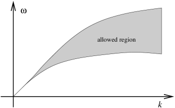
Figure 2: Fourier transform of EOM. The support of solutions has to lie in the shaded region.

We have to note, however that even if this is true, there is no guarantee that a dispersion relation with corrections to the linear term makes sense as an approximate description for long wavelength. We tried to visualize this in figure 3. So, to conclude, it is very plausible that a nonlinear dispersion relation will turn out to be a good approximate description of the physical contents of (5.3) for long wavelength in this sense. But issues such as the one depicted in figure 3 definitely merit further studies.

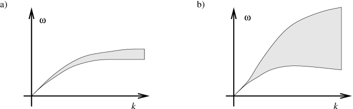
Figure 3: Can higher order corrections to the dispersion relation be given? a) Yes, approximately. b) No, there is no meaningful notion of dispersion relation beyond linear order

Let us now turn to the practical question of how a nonlinear dispersion relation can actually be computed from (5.3). A simple model that displays some of the complications due to the vertex dependence of the coefficients in (5.3), but can nevertheless be treated with analytical methods, can be obtained from (5.1) in the following way: Upon setting $m=1$ and $K=l^{-2}$, the Hamiltonian (5.1) can be interpreted as that of a scalar field propagating on a one dimensional lattice with lattice spacing $l$. Now we partly remove the assumption of a constant lattice spacing by replacing $l$ by $l_{z}$ – the distance between the lattice point labelled by $z$ and the one labelled by $z+1$ – but still assume periodicity on a large scale,

$$l_{z}=l_{N+z}\quad\text{for all }\quad z\in\mathbb{Z}$$

for some $N\in\mathbb{N}$. It turns out that the dispersion relation for this system has several branches and the small $k$ behavior of the acoustic branch is given by

$$\omega_{\text{ac}}^{2}(k)=\frac{\langle\langle l\rangle\rangle{}^{2}}{\langle\langle l^{2}\rangle\rangle{}}\left\lvert k\right\rvert^{2}+\left(\frac{1}{L^{2}}\frac{\langle\langle l\rangle\rangle{}^{6}}{\langle\langle l^{2}\rangle\rangle{}^{3}}\sum_{i<j}c_{ij}l_{i}^{2}l_{j}^{2}-\frac{L^{2}}{12}\frac{\langle\langle l\rangle\rangle{}^{2}}{\langle\langle l^{2}\rangle\rangle{}}\right)\left\lvert k\right\rvert^{4}+O\left(\left\lvert k\right\rvert^{6}\right).$$ (5.5)

Here,

$$L=\sum_{n=0}^{N-1}l_{n},\qquad c_{ij}=(j-i)[N-(j-i)],\quad\text{ and }\langle\langle l\rangle\rangle{}=\frac{1}{N}\sum_{n=0}^{N-1}l_{n}\quad\text{ etc.}$$

As we we have indicated by means of notation, it is instructive to view the $l_{i},i=0,\ldots,N-1$ as independent random variables. The moments of the corresponding distribution determine the dispersion relation (5.5). In each order in $k$, corrections are present as compared to the case of constant lattice spacing. Note in particular that the phase velocity $\lim_{k\rightarrow 0}\omega(k)/k$ can be smaller than one.

It is remarkable how subtle the dependence of the dispersion relation on the distribution of the lengths is already in this simple model. Although we do not have a proof, it is plausible that qualitatively, the above formula extends to higher dimensions, where analytical proofs get much harder. For more information about the model as well as a proof of (5.5) we refer the reader to [57] or [58], for a beautiful numerical analysis of similar models in two dimensions to [59].

The discussion of the one dimensional model given above shows how complicated an exact analysis of the equations of motion is already in simple cases. Since the models

$$H^{\Psi_{\text{flat}}}=\frac{1}{2}\sum_{v,v^{\prime},l,l^{\prime}}p_{l}(v)P_{\Psi_{\text{flat}}}((v,l),(v^{\prime},l^{\prime}))p_{l^{\prime}}(v^{\prime})+q_{l}(v)Q_{\Psi_{\text{flat}}}(v,l),(v^{\prime},l^{\prime}))q_{l^{\prime}}(v^{\prime}),$$ (5.6)

that one obtains from QGR are more complicated, it is useful to explore a less precise but easier route towards dispersion relations. The idea which we would like to advocate is to replace (5.6) by a simpler Hamiltonian which

• is a good approximation of (5.6) for slowly varying $q$ and $p$ and

• is simple enough such that the EOM can be solved exactly.

This idea underlies also the works [21] and [22] and, at a rather simple level, is the basis for the recovery of continuum elasticity theory from the atomic description in solid state physics (see for example [60]).

We will now propose a replacement for (5.6) fulfilling the above requirements. In the long wavelength regime, we can revert to the continuum picture, i.e. replace the lattice fields $q_{l}(v),p_{l}(v)$ by $q_{l}(\vec{x}(v)),p_{l}(\vec{x}(v))$, where now $q_{l},p_{l}:\Sigma\rightarrow\mathbb{C}$.

We should however take care that information about the lattice is at least partially encoded in the continuum theory. To this end, we Taylor expand the (now continuum) fields in the Hamiltonian up to a certain order. For example, we would make the replacement

$$q_{l}(\vec{x}(v))Q_{\Psi}((v,l),(v^{\prime},l^{\prime}))q_{l^{\prime}}(\vec{x}(v^{\prime}))\\ \xrightarrow{\hskip 21.52771pt}q_{l}(\vec{x}(v))Q_{\Psi}((v,l),(v^{\prime},l^{\prime}))\Big{[}b^{i}(v,v^{\prime})\partial_{i}q_{l^{\prime}}(\vec{x}(v))+\frac{1}{2!}b^{i}(v,v^{\prime})b^{j}(v,v^{\prime})\partial_{i}\partial_{j}q_{l^{\prime}}(\vec{x}(v))+\ldots\Big{]}$$

where $b^{i}(v,v^{\prime})\doteq\vec{x}(v^{\prime})-\vec{x}(v)$. Even if we terminate the Taylor expansion after a few terms, the resulting Hamiltonian will be an excellent approximation to the original one, provided $p$ and $q$ change only very little from vertex to vertex, our standing assumption in the whole procedure.

Now we will eliminate the spacial dependence of the coefficients, which was the main difficulty in dealing with the original Hamiltonian (5.6), by replacing them by their averages over all vertices of the graph. This can be justified as follows: If the fields $p,q$ are varying considerably only on length scales much larger then some macroscopic scale $L$, it is a very good approximation to replace the vertex dependent coefficients in the Hamiltonian by their averages over the vertices in regions of dimension $L^{3}$. On the other hand, as we have said before, a good semiclassical $\Psi_{\text{flat}}$ state will insure that the system described by (5.6) has the symmetries of flat space at least at large distances. One way to state this more precisely is that the average of the coefficients appearing in (5.6) over vertices in regions with characteristic dimension $L^{3}$ or larger, is independent of the region to a good approximation. Therefore we can indeed replace the vertex dependent coefficients by their averages over all vertices.

Let us again give an example for a typical term in the Hamiltonian:

$$\sum_{v^{\prime}}Q((v,l),(v^{\prime},l^{\prime}))b^{a_{1}}(v,v^{\prime})\ldots b^{a_{n}}(v,v^{\prime})=:F^{a_{1}\ldots a_{n}}(v,l,l^{\prime})\xrightarrow{\hskip 21.52771pt}\langle\langle F^{a_{1}\ldots a_{n}}(\cdot,l,l^{\prime})\rangle\rangle{}$$

where we have introduced the graph average

$$\langle\langle F^{a_{1}\ldots a_{n}}(\cdot,l,l^{\prime})\rangle\rangle{}\doteq\frac{1}{N}\sum_{v}F^{a_{1}\ldots a_{n}}(v,l,l^{\prime}),$$ (5.7)

$N$ being the number of vertices of the graph $\Psi_{\text{flat}}$ is based on. In case we are dealing with an infinite number of vertices, the definition (5.7) has to be replaced by the limit of averages over finite but larger and larger numbers of points.

Finally we can replace the sum over vertices of (5.4) by an integral. We thus end up with a Hamiltonian for a continuum field theory on $\Sigma$ and the coefficients of the fields being constant. Therefore the equations of motion of the theory admit plane waves as solutions, and their dispersion relation can be computed and discussed. This dispersion relation should describe the physical content of (5.6) for low energies (large wavelength).

To justify our procedure, let us point out again, that it uses both assumptions (large wavelength – homogeneity and isotropy of the state on large scales) that seem essential from physical considerations, to recover a dispersion relation from (5.6), enter in a transparent way. Also, if we apply the procedure outlined above to the simple regular lattice system (5.1), we recover, order by order, the nonlinear dispersion relation (5.2). Thus, at least in this example, the simplified continuum theory still captures the information about the lattice to any desired order of accuracy.

In the companion paper [1] we will elaborate on the procedure described above and apply it to derive approximate dispersion relations from the Hamiltonians constructed in this paper, evaluated in the gauge theory coherent states of [9].

6 Summary and Outlook

The goal of the present work was to begin investigations of the structure and semiclassical limit of the theory obtained by coupling matter fields to QGR. A basic assumption that we made was that the complicated dynamics of a full theory could be approximated by treating the matter parts in the Hamilton constraint of the full theory as Hamiltonians generating the matter dynamics and by the use of semiclassical states in the gravitational sector.

Using this assumption we obtained the following results:

1. We have proposed quantum theories of scalar, electromagnetic and fermionic fields coupled to QGR. The dynamics of these theories is generated by a Hamiltonian in the same way as in ordinary QFT. Consequently we were able to identify approximate $n$-particle states which correspond to the usual Fock states for matter fields propagating on classical geometries. In other respects, the theories are very different from ordinary QFT, thus reflecting basic properties of QGR:

   • The basic excitations of the gravitational field in QGR are concentrated on graphs. The requirement of diffeomorphism invariance forces the matter degrees of freedom to be confined to the same graph as the gravitational field. The matter fields are therefore bound to become quantum fields propagating on a discrete structure.

   • In ordinary QFT, the background metric enters the definition of the ground state and the commutation relations of the fields. In QGR on the other hand, the geometry is a dynamical variable, represented by suitable operators. A QFT coupled to QGR therefore has to contain these operators in its very definition. This is reflected in the theories of section 4 by the fact that their annihilation and creation operators act on both, the one particle Hilbert space of the matter fields and the Hilbert space of the geometry.

   We also showed how a “QFT on curved space-time limit” can be obtained from this theory, using a semiclassical state of the gravitational field.

2. We have discussed how modified dispersion relations for the matter fields arise in the context of QGR and motivated a method for computing them from the (partial) expectation values of the quantum matter Hamiltonians in a semiclassical state.

Certainly, the present work can only be regarded as a first step towards a better understanding of the interaction of matter and quantum gravity. In future work, the assumptions that have been used should be removed, or their validity confirmed.

On the other hand, application of the results of the present work can be envisioned. For example, it will be very interesting to see, whether the methods used in the present work can also be applied to investigate how gravitons arise in the semiclassical regime of QGR. This will be the topic of [19]. As another application, the companion paper [1] contains a calculation of corrections to the standard dispersion relations for the scalar and the electromagnetic field due to QGR.

To summarize, the interaction of quantum matter and quantum gravity is a fascinating but, alas, very complicated topic, of which a good understanding still has to be gained. We hope that the present work illuminates the difficulties encountered in this endeavor and also contains some first, albeit small, steps towards its completion.


Acknowledgements

It is a pleasure for us to thank Abhay Ashtekar, Luca Bombelli, Arundhati Dasgupta, Rodolfo Gambini, Jurek Lewandowski, Fotini Markopoulou Kalamara, Hugo Morales-Tecotl, Jorge Pullin, and Oliver Winkler for numerous valuable discussions. We also thank the Center for Gravitational Physics of The Pennsylvania State University, where part of this work was completed, for warm hospitality. T.T. was supported in part by NSF grant PHY 0090091 to The Pennsylvania State University.

H.S. also gratefully acknowledges the splendid hospitality at the Universidad Autonoma Metropolitana Iztapalapa, Mexico City, and at the University of Mississippi, as well as the financial support by the Studienstiftung des Deutschen Volkes.

Appendix: Kinematical vs. Dynamical Coherent States: A Simple Example

In systems with constraints linear in the basic variables, the expectation values of Dirac observables in a coherent state in the kinematical Hilbert space equal those in a dynamical coherent state, provided that both states are chosen to be peaked around the same point in the constrained phase space. This does not hold true anymore for systems with nonlinear constraints. One expects, however that the discrepancies between the expectation values on the kinematical and on the dynamical level will at least be small. In this appendix, we demonstrate that this is true for a simple quantum mechanical model system with a nonlinear constraint: A system of two coupled harmonic oscillators.

Let the Hamiltonian of the harmonic oscillator be given as

$$H=\frac{1}{2}\left(\frac{p^{2}}{m}+m\omega^{2}q^{2}\right).$$

It is well known that it can be quantized in terms of annihilation and creation operators $\widehat{a},\widehat{a}^{\dagger}$, $\,\left[\widehat{a},\widehat{a}^{\dagger}\right]=1$ on the Fock space $\mathcal{H}$ over $\mathbb{C}$. $\widehat{a}$ is the quantization of the classical quantity

$$z=\sqrt{\frac{m\omega}{2\hbar}}\left(q+i\frac{p}{m\omega}\right).$$

A basis of $\mathcal{H}$ is given by the eigenvectors of the number operator $\widehat{N}=\widehat{a}^{\dagger}\widehat{a}$ and will be denoted by $\lvert n\rangle$. The coherent states for the harmonic oscillator are defined as

$$\lvert z\rangle=\exp\left(-\frac{\left\lvert z^{2}\right\rvert}{2t}\right)\sum_{n=0}^{\infty}\frac{z^{n}}{\sqrt{t^{n}n!}}\lvert n\rangle,\qquad z\in\mathbb{C}$$

A system of two harmonic oscillators can be quantized on the tensor product $\mathcal{H}^{\text{kin}}\doteq\mathcal{H}\otimes\mathcal{H}$, the annihilation operators of the respective oscillators are given by

$$\widehat{a}_{1}\doteq\widehat{a}\otimes 1,\qquad\qquad\widehat{a}_{2}\doteq 1\otimes\widehat{a},$$

and similarly for the number operators $\widehat{N}_{1},\widehat{N}_{2}$. Analogously we have

$$\lvert n_{1},n_{2}\rangle\doteq\lvert n_{1}\rangle\otimes\lvert n_{2}\rangle,\qquad\lvert z_{1},z_{2}\rangle\doteq\lvert z_{1}\rangle\otimes\lvert z_{2}\rangle,\qquad n_{1},n_{2}\in\mathbb{N}_{0},\,z_{1},z_{2}\in\mathbb{C}$$

and these vectors form dense subsets in $\mathcal{H}^{\text{kin}}$.

Let us now impose the constraint $C\doteq N_{1}-N_{2}$ forcing the energies of the two oscillators to be equal. The kinematical phase space can be labeled by $(z_{1},z_{2})\in\mathbb{C}^{2}$, the physical phase space by $z\in\mathbb{C}$, where the embedding of the latter in the former is given by

$$\left\lvert z\right\rvert=\left\lvert z_{1}\right\rvert=\left\lvert z_{2}\right\rvert,\qquad z\left\lvert z\right\rvert=z_{1}z_{2}.$$ (A.1)

The quantization of the constraint is simply

$$\widehat{C}=\widehat{N}_{1}-\widehat{N}_{2},$$ (A.2)

the physical subspace of $\mathcal{H}^{\text{kin}}$ is given by

$$\mathcal{H}^{\text{phys}}=\overline{\operatorname{span}\left\{\lvert n,n\rangle,\,n\in\mathbb{N}_{0}\right\}}.$$

On this subspace, a new annihilation operator can be defined by

$$\widehat{a}_{\otimes}\doteq\widehat{a}_{1}\widehat{N}_{1}^{-\frac{1}{4}}\widehat{a}_{2}\widehat{N}_{2}^{-\frac{1}{4}}$$

on $\operatorname{span}\{\lvert n,n\rangle,\,n\in\mathbb{N}\}$ and $\widehat{a}_{\otimes}\lvert 0,0\rangle\doteq 0$. It fulfills $\left[\widehat{a}_{\otimes},\widehat{a}_{\otimes}^{\dagger}\right]=1$. Therfore we can define physical coherent states as

$$\lvert z\rangle_{\otimes}=\exp\left(-\frac{\left\lvert z^{2}\right\rvert}{2}\right)\sum_{n=0}^{\infty}\frac{z^{n}}{n!}(\widehat{a}_{\otimes}^{\dagger})^{n}\lvert 0,0\rangle.$$

These are to be compared with the kinematical coherent states $\lvert z_{1},z_{2}\rangle$, bearing in mind the identification (A.1).

Let us consider the expectation values of the Dirac observables $\widehat{a}_{1}\widehat{a}_{2}$ and $\widehat{N}_{1}$ and more complicated ones constructed from them. We start with $N_{1}$: Clearly

$$\langle\widehat{N}_{1}\rangle_{\lvert z_{1},z_{2}\rangle}=\left\lvert z_{1}\right\rvert^{2}=\left\lvert z\right\rvert^{2}.$$

On the other hand, one finds

$$\langle\widehat{N}_{1}\rangle_{\lvert z\rangle_{\otimes}}=\left\lvert z\right\rvert^{2},$$

so in this case the expectation values agree exactly. Now we turn to $\widehat{a}_{1}\widehat{a}_{2}$: In the kinematical coherent states

$$\langle\widehat{a}_{1}\widehat{a}_{2}\rangle_{\lvert z_{1},z_{2}\rangle}=z_{1}z_{2}=z\left\lvert z\right\rvert.$$ (A.3)

The expectation value in the physical coherent states is

$$\langle\widehat{a}_{1}\widehat{a}_{2}\rangle_{\lvert z\rangle_{\otimes}}=z\exp\left(-\left\lvert z\right\rvert^{2}\right)\sum_{n=0}^{\infty}\sqrt{n+1}\frac{\left\lvert z\right\rvert^{2n}}{n!}.$$ (A.4)

The sum in this formula can not be determined in terms of elementary functions. We can, however study its behavior for large $\left\lvert z\right\rvert$. To this end, let us define the function

$$F_{\alpha}(b)\doteq\sum_{n=1}^{\infty}\frac{b^{n}}{n!}\left(\frac{n}{b}\right)^{\alpha}.$$ (A.5)

Then we can write (A.4) as

$$\langle\widehat{a}_{1}\widehat{a}_{2}\rangle_{\lvert z\rangle_{\otimes}}=z\left\lvert z\right\rvert e^{-b}F_{\frac{3}{2}}(b)$$

where $b=\left\lvert z\right\rvert^{2}$. To obtain an asymptotic formula for $F_{\alpha}(b)$ for large $b$, we approximate the factorial in (A.5) by Stirlings formula and the discrete sum by an integral. We find

$$F_{\alpha}(b)\approx\sqrt{\frac{b}{2\pi}}\int_{0}^{\infty}x^{\alpha-\frac{1}{2}}\exp\left(-bx(\ln x-1)\right)\,dx$$

The asymptotic behavior of this integral can be obtained by saddle point methods (see for example [61]). We obtain

$$F_{\alpha}(b)=e^{b}\left[1+\frac{1}{b}\left(\frac{1}{2}(\alpha-\frac{1}{2})^{2}-\frac{1}{8}\right)+O(b^{-2})\right].$$ (A.6)

Therefore the expectation value (A.4) is

$$\langle\widehat{a}_{1}\widehat{a}_{2}\rangle_{\lvert z\rangle_{\otimes}}=z\left\lvert z\right\rvert\left(1+\frac{3}{8}\frac{1}{\left\lvert z\right\rvert^{2}}+O(\left\lvert z\right\rvert^{-4})\right).$$

Comparing this with (A.3), we see that the expectation values in kinematical and physical coherent states disagree by a term of order $1$. This is a small correction if $\left\lvert z\right\rvert$ is large.

Similar results can be obtained for more complicated functions of the Dirac observables. Consider for example the operator $\widehat{a}_{\otimes}$. It can be written as $\widehat{a}_{1}\widehat{a}_{2}\widehat{N}_{1}^{-1/4}\widehat{N}_{2}^{-1/4}$. In this case, the expectation value in the physical coherent states is trivial:

$$\langle\widehat{a}_{\otimes}\rangle_{\lvert z\rangle_{\otimes}}=z.$$

On the other hand, we find

$$\langle\widehat{a}_{\otimes}\rangle_{\lvert z_{1},z_{2}\rangle}=\frac{z_{1}}{\sqrt{\left\lvert z_{1}\right\rvert}}\frac{z_{2}}{\sqrt{\left\lvert z_{2}\right\rvert}}e^{-b_{1}}e^{-b_{2}}F_{\frac{3}{4}}(b_{1})F_{\frac{3}{4}}(b_{2})$$

where $b_{i}=\left\lvert z_{i}\right\rvert^{2}$. Using (A.6) this can be simplified to

$$\langle\widehat{a}_{\otimes}\rangle_{\lvert z_{1},z_{2}\rangle}=z\left(1-\frac{3}{16}\frac{1}{\left\lvert z\right\rvert^{2}}+O(\left\lvert z\right\rvert^{-4})\right).$$

Summarizing, we find that in the simple example of two harmonic oscillators coupled by the constraint (A.2), expectation values of Dirac observables in both, kinematical and physical coherent states, can be computed to any desired order of accuracy. For some observables, these expectation values agree. For others, there are $\hbar$-corrections. This indicates that kinematical coherent states always give the same answer to zeroth order as the dynamical ones and that the first corrections differ by a constant of proportionality of order unity so that at least qualitatively we get a good idea of which corrections to expect in the exact theory.

References

- [1] H. Sahlmann and T. Thiemann, Towards the QFT on curved spacetime limit of QGR. II: A concrete implementation, http://arXiv.org/abs/gr-qc/0207031.
- [2] T. Thiemann, Introduction to modern canonical quantum general relativity, http://arXiv.org/abs/gr-qc/0110034.
- [3] C. Rovelli, Loop quantum gravity, Living Rev. Rel. 1 (1998) 1 [http://arXiv.org/abs/gr-qc/9710008].
- [4] G. T. Horowitz, Quantum gravity at the turn of the millennium, http://arXiv.org/abs/gr-qc/0011089.
- [5] C. Rovelli, Strings, loops and others: A critical survey of the present approaches to quantum gravity, http://arXiv.org/abs/gr-qc/9803024.
- [6] C. Rovelli, The century of the incomplete revolution: Searching for general relativistic quantum field theory, J. Math. Phys. 41 (2000) 3776–3800 [http://arXiv.org/abs/hep-th/9910131].
- [7] A. Ashtekar, C. Rovelli and L. Smolin, Weaving a classical geometry with quantum threads, Phys. Rev. Lett. 69 (1992) 237–240 [http://arXiv.org/abs/hep-th/9203079].
- [8] L. Bombelli, Statistical geometry of random weave states, http://arXiv.org/abs/gr-qc/0101080.
- [9] T. Thiemann, Gauge field theory coherent states (GCS). I: General properties, Class. Quant. Grav. 18 (2001) 2025–2064 [http://arXiv.org/abs/hep-th/0005233].
- [10] T. Thiemann and O. Winkler, Gauge field theory coherent states (GCS). II: Peakedness properties, Class. Quant. Grav. 18 (2001) 2561–2636 [http://arXiv.org/abs/hep-th/0005237].
- [11] T. Thiemann and O. Winkler, Gauge field theory coherent states (GCS) III: Ehrenfest theorems, Class. Quant. Grav. 18 (2001) 4629–4682 [http://arXiv.org/abs/hep-th/0005234].
- [12] J. Iwasaki and C. Rovelli, Gravitons from loops: Nonperturbative loop space quantum gravity contains the graviton physics approximation, Class. Quant. Grav. 11 (1994) 1653–1676.
- [13] J. Iwasaki and C. Rovelli, Gravitons as embroidery on the weave, Int. J. Mod. Phys. D1 (1993) 533–557.
- [14] A. Ashtekar, C. Rovelli and L. Smolin, Gravitons and loops, Phys. Rev. D44 (1991) 1740–1755 [http://arXiv.org/abs/hep-th/9202054].
- [15] M. Varadarajan, Gravitons from a loop representation of linearised gravity, http://arXiv.org/abs/gr-qc/0204067.
- [16] M. Varadarajan, Photons from quantized electric flux representations, Phys. Rev. D64 (2001) 104003 [http://arXiv.org/abs/gr-qc/0104051].
- [17] M. Varadarajan, Fock representations from U(1) holonomy algebras, Phys. Rev. D61 (2000) 104001 [http://arXiv.org/abs/gr-qc/0001050].
- [18] A. Ashtekar and J. Lewandowski, Relation between polymer and Fock excitations, Class. Quant. Grav. 18 (2001) L117–L128 [http://arXiv.org/abs/gr-qc/0107043].
- [19] T. Thiemann, “Gravitons from quantum general relativity.” in preparation.
- [20] G. Amelino-Camelia, Quantum-gravity phenomenology: Status and prospects, http://arXiv.org/abs/gr-qc/0204051.
- [21] R. Gambini and J. Pullin, Nonstandard optics from quantum spacetime, Phys. Rev. D59 (1999) 124021 [http://arXiv.org/abs/gr-qc/9809038].
- [22] J. Alfaro, H. A. Morales-Tecotl and L. F. Urrutia, Quantum gravity corrections to neutrino propagation, Phys. Rev. Lett. 84 (2000) 2318–2321 [http://arXiv.org/abs/gr-qc/9909079].
- [23] J. Alfaro, H. A. Morales-Tecotl and L. F. Urrutia, Loop quantum gravity and light propagation, http://arXiv.org/abs/hep-th/0108061.
- [24] J. Alfaro and G. Palma, Loop quantum gravity corrections and cosmic rays decays, http://arXiv.org/abs/hep-th/0111176.
- [25] T. Thiemann, Kinematical Hilbert spaces for fermionic and Higgs quantum field theories, Class. Quant. Grav. 15 (1998) 1487–1512 [http://arXiv.org/abs/gr-qc/9705021].
- [26] T. Thiemann, QSD III: Quantum constraint algebra and physical scalar product in quantum general relativity, Class. Quant. Grav. 15 (1998) 1207–1247 [http://arXiv.org/abs/gr-qc/9705017].
- [27] T. Thiemann, QSD V: Quantum gravity as the natural regulator of matter quantum field theories, Class. Quant. Grav. 15 (1998) 1281–1314 [http://arXiv.org/abs/gr-qc/9705019].
- [28] T. Thiemann, Quantum spin dynamics (QSD), Class. Quant. Grav. 15 (1998) 839–873 [http://arXiv.org/abs/gr-qc/9606089].
- [29] T. Thiemann, Quantum spin dynamics (QSD) II, Class. Quant. Grav. 15 (1998) 875–905 [http://arXiv.org/abs/gr-qc/9606090].
- [30] C. Di Bartolo, R. Gambini, J. Griego and J. Pullin, Canonical quantum gravity in the Vassiliev invariants arena. I: Kinematical structure, Class. Quant. Grav. 17 (2000) 3211–3238 [http://arXiv.org/abs/gr-qc/9911009].
- [31] C. Di Bartolo, R. Gambini, J. Griego and J. Pullin, Canonical quantum gravity in the Vassiliev invariants arena. II: Constraints, habitats and consistency of the constraint algebra, Class. Quant. Grav. 17 (2000) 3239–3264 [http://arXiv.org/abs/gr-qc/9911010].
- [32] M. Bojowald, Isotropic loop quantum cosmology, Class. Quant. Grav. 19 (2002) 2717–2742 [http://arXiv.org/abs/gr-qc/0202077].
- [33] M. Bojowald, The inverse scale factor in isotropic quantum geometry, Phys. Rev. D64 (2001) 084018 [http://arXiv.org/abs/gr-qc/0105067].
- [34] A. Ashtekar, J. Lewandowski, D. Marolf, J. Mourao and T. Thiemann, Quantization of diffeomorphism invariant theories of connections with local degrees of freedom, J. Math. Phys. 36 (1995) 6456–6493 [http://arXiv.org/abs/gr-qc/9504018].
- [35] C. Rovelli, What is observable in classical and quantum gravity?, Class. Quant. Grav. 8 (1991) 297–316.
- [36] C. Rovelli, Quantum reference systems, Class. Quant. Grav. 8 (1991) 317–332.
- [37] M. O. Scully and M. S. Zubairy, Quantum optics. Cambridge University Press, 1997.
- [38] T. Thiemann, Complexifier coherent states for quantum general relativity, http://arXiv.org/abs/gr-qc/0206037.
- [39] N. H. Christ, R. Friedberg and T. D. Lee, Random lattice field theory: General formulation, Nucl. Phys. B202 (1982) 89.
- [40] N. H. Christ, R. Friedberg and T. D. Lee, Gauge theory on a random lattice, Nucl. Phys. B210 (1982) 310.
- [41] N. H. Christ, R. Friedberg and T. D. Lee, Weights of links and plaquettes in a random lattice, Nucl. Phys. B210 (1982) 337.
- [42] G. Immirzi, Quantum gravity and Regge calculus, Nucl. Phys. Proc. Suppl. 57 (1997) 65–72 [http://arXiv.org/abs/gr-qc/9701052].
- [43] J. F. Barbero, Reality conditions and Ashtekar variables: A different perspective, Phys. Rev. D51 (1995) 5498–5506 [http://arXiv.org/abs/gr-qc/9410013].
- [44] N. Biggs, Algebraic Graph Theory. Cambridge University Press, Cambridge, 2 ed., 1993.
- [45] D. Stauffer and A. Aharony, Introduction to Percolation Theory. Taylor and Francis, London, 2 ed., 1994.
- [46] D. Cvetovic, M. Doob and H. Sachs, Spectra of Graphs. Academic Press, New York, 1979.
- [47] M. Gaul and C. Rovelli, A generalized Hamiltonian constraint operator in loop quantum gravity and its simplest Euclidean matrix elements, Class. Quant. Grav. 18 (2001) 1593–1624 [http://arXiv.org/abs/gr-qc/0011106].
- [48] C. Rovelli and L. Smolin, Discreteness of area and volume in quantum gravity, Nucl. Phys. B442 (1995) 593–622 [http://arXiv.org/abs/gr-qc/9411005].
- [49] A. Ashtekar and J. Lewandowski, Quantum theory of geometry. II: Volume operators, Adv. Theor. Math. Phys. 1 (1998) 388 [http://arXiv.org/abs/gr-qc/9711031].
- [50] T. Thiemann and O. Winkler, Gauge field theory coherent states (GCS). IV: Infinite tensor product and thermodynamical limit, Class. Quant. Grav. 18 (2001) 4997–5054 [http://arXiv.org/abs/hep-th/0005235].
- [51] P. Hasenfratz, The theoretical background and properties of perfect actions, http://arXiv.org/abs/hep-lat/9803027.
- [52] S. Hauswirth, Perfect discretizations of differential operators, http://arXiv.org/abs/hep-lat/0003007.
- [53] P. Hasenfratz et. al., The construction of generalized Dirac operators on the lattice, Int. J. Mod. Phys. C12 (2001) 691–708 [http://arXiv.org/abs/hep-lat/0003013].
- [54] B. Hall, The Segal-Bargmann “coherent state” transform for compact Lie groups, Journ. Funct. Analysis 122 (1994) 103–151.
- [55] A. Ashtekar, J. Lewandowski, D. Marolf, J. Mourao and T. Thiemann, Coherent state transforms for spaces of connections, J. Funct. Anal. 135 (1996) 519–551 [http://arXiv.org/abs/gr-qc/9412014].
- [56] T. Thiemann, Quantum spin dynamics (QSD). VII: Symplectic structures and continuum lattice formulations of gauge field theories, Class. Quant. Grav. 18 (2001) 3293–3338 [http://arXiv.org/abs/hep-th/0005232].
- [57] H. Sahlmann, Coupling Matter to Loop Quantum Gravity. PhD thesis, Universität Potsdam, 2002.
- [58] H. Sahlmann and T. Thiemann, “Waves on inhomogenous lattices - a model for light propagation in quantum general relativity.” in preparation.
- [59] A. Tanguy, J. P. Wittmer, F. Leonforte and J.-L. Barrat, Continuum limit of amorphous elastic bodies: A finite-size study of low frequency harmonic vibrations, http://arXiv.org/abs/cond-mat/0204258.
- [60] N. W. Ashcroft and N. Mermin, Solid State Physics, ch. 22. Harcourt Brace College Publishers, 1976.
- [61] N. Bleistein and R. Handelsman, Asymptotic Expansion of Integrals. Dover Publications, New York, 1986.