Late-time particle creation from gravitational collapse to an extremal Reissner-Nordström black hole

Abstract

We investigate the late-time behavior of particle creation from an extremal Reissner-Nordstrom (RN) black hole formed by gravitational collapse. We calculate explicitly the particle flux associated with a massless scalar field at late times after the collapse. Our result shows that the expected number of particles in any wave packet spontaneously created from the “in” vacuum state approaches zero faster than any inverse power of time. This result confirms the traditional belief that extremal black holes do not emit particles. We also calculate the expectation value of the stress energy tensor in a 1+1 RN black hole and show that it also drops to zero at late times. Some comments on previous work by other authors are provided.

1 Introduction

As a quantum effect, particle production by black holes (Hawking radiation) was widely studied since the 1970s [1][2][3]. It is well known that black holes emit particles with the same spectrum as a blackbody with a temperature $T=\hbar\kappa/2\pi k$, where $\kappa$ is the surface gravity of the black hole and $k$ is the Boltzmann’s constant. The Hawking radiation can be derived for a spacetime appropriate to a collapsing body. At a late stage, the collapse settles down to a stationary black hole. Since spacetime is asymptotically flat at both past infinity ${\mycal I}^{-}$ and future infinity ${\mycal I}^{+}$, we can define the “in” and “out” vacuum states, respectively. If the two vacuum states are distinct from one another, particles will be detected at future infinity when the initial state is in “in” vacuum. If such creation takes place at a steady rate at late times, it indicates that those particles are produced from the stationary black hole instead of from the collapse phase.

Although the standard derivations of Hawking radiation only deal with nonextremal black holes, it is generally accepted that extremal black holes have zero temperature and consequently no particles are created. However, Liberati, et al. [4] pointed out that the generalization to extremal black holes from nonextremal black holes is not trivial. One important difference is that the Kruskal transformation for non-extremal black holes, which plays a crucial role in computing the particle creation, breaks down for extremal black holes.

The arguments in [4] are reviewed briefly here as follows. Start with the usual form of the Reissner-Nordström (RN) geometry with parameters $Q$ and $M$

$$ds^{2}=-\left(1-\frac{2M}{r}+\frac{Q^{2}}{r^{2}}\right)dt^{2}+\left(1-\frac{2M}{r}+\frac{Q^{2}}{r^{2}}\right)^{-1}dr^{2}+r^{2}d\Omega^{2},$$ (1)

where $d\Omega^{2}$ is the metric on the unit sphere. The tortoise coordinate $r_{*}(Q,M)$ is given by

$$r_{*}(Q,M)=\int\frac{dr}{1-2M/r+Q^{2}/r^{2}}.$$ (2)

In the nonextremal case $|Q|<M$,

$$r_{*}(Q,M)=r+\frac{1}{2\sqrt{M^{2}-Q^{2}}}\left[r^{2}_{+}\ln(r-r_{+})-r^{2}_{-}\ln(r-r_{-})\right]$$ (3)

where $r_{\pm}=M\pm\sqrt{M^{2}-Q^{2}}$. Define the retarded time $u$ and advanced time $v$ as

$$u = t-r_{*},$$

$$v = t+r_{*}.$$ (4)

The well-known Kruskal transformation for the nonextremal case is

$$U = -e^{-\kappa u}\leftrightarrow u=-\frac{1}{\kappa}\ln(-U),$$ (5)

$$V = e^{\kappa v}\leftrightarrow v=\frac{1}{\kappa}\ln(V),$$ (6)

where $U$ and $V$ are regular across the past and future horizons of the extended spacetime. In the extremal case $|Q|=M$, the right-hand side of Eq. (3) appears to yield the indeterminate form $0/0$. This can be fixed by setting $|Q|=M$ in Eq. (2) before integrating. Thus,

$$r_{*}(M,M)=r+2M\left(\ln(r-M)-\frac{M}{2(r-M)}\right).$$ (7)

Since $\kappa=0$ when $|Q|=M$, the Kruskal transformation (5) and (6) breaks down for the extremal case. A generalization of the Kruskal transformation to the extremal RN black hole is [4]

$$u = -4M\left(\ln(-U)+\frac{M}{2U}\right),$$ (8)

$$v = 4M\left(\ln(V)-\frac{M}{2V}\right).$$ (9)

We shall show, in section 2.2, that Eq. (8) defines a smooth extension. However, Liberati, et al. [4] actually used a simplified extension

$$u = -\frac{2M^{2}}{U},$$ (10)

which, as we will show later, is not a smooth extension (Eq. (10) is essentially the same extension introduced by Lake [5]). By using this extension, Liberati, et al. [4] calculated the Bogoliubov coefficients associated with plane wave solutions of a massless scalar field in a two-dimensional Minkowski spacetime with a moving mirror (serving as a timelike boundary) which is physically equivalent to a (1+1)-dimensional model of an extremal RN spacetime formed from a collapsing star. The result shows that the Bogoliubov coefficients are nonzero, indicating that particles are created in the late stages of collapse. Further calculations in [4] also show that the expectation value of the stress-energy-momentum tensor is zero and its variance vanishes as a power law at late times. The authors thereby claim that the extremal black hole does not behave as a thermal object and cannot be regarded as the thermodynamic limit of a nonextremal black hole.

However, the major deficiency in the analysis of [4] is the use of unnormalized plane-wave solutions. These kinds of solutions have been used for nonextremal cases [6][7][8]. The Bogoliubov coefficients $\beta_{\omega\omega^{\prime}}$ in [4] have the form

$$\beta_{\omega\omega^{\prime}}\sim\sqrt{\frac{\omega^{\prime}}{\omega}}\int_{0}^{\infty}e^{-i\omega^{\prime}v+\frac{ia\omega}{v}}dv.$$ (11)

The integrand is oscillated with constant amplitude. So the integral is not well-defined. The result

$$\beta_{\omega\omega^{\prime}}\sim K_{1}(2\sqrt{a\omega\omega^{\prime}})$$ (12)

given in [4], which was originally calculated by Davis and Fulling [8], was obtained by Wick rotation, i.e., integrating along the imaginary axis. But this Wick rotation is unjustified since the integrand does not fall off at large radius on the complex plane. Since the spectrum of particle number created from the vacuum is

$$<N_{\omega}>=\int_{0}^{\infty}|\beta_{\omega\omega^{\prime}}|^{2}d\omega^{\prime}$$ (13)

and $K_{1}(z)\sim 1/z$ for $z\rightarrow 0$ [12], the number of particle is divergent. The authors interpret the infinity as an accumulation after an infinite time. The Kruskal extension (10) was used in deriving Eq. (11). If we use the smooth extension (8) instead, the Bogoliubov coefficients would be

$$\beta_{\omega\omega^{\prime}}\sim\sqrt{\frac{\omega^{\prime}}{\omega}}\int_{0}^{\infty}e^{-i\omega^{\prime}v+\frac{ia\omega}{v}}e^{-4iM\omega\ln(v)}dv$$ (14)

and by using the same Wick rotation (also unjustified), it follows that

$$\beta_{\omega\omega^{\prime}}\sim\omega^{\prime 2iM\omega}K_{1-4iM\omega}(2\sqrt{a\omega\omega^{\prime}}).$$ (15)

For small $z$, $K_{1-4iM\omega}(z)\approx\frac{1}{2}\Gamma(1-4iM\omega)(\frac{z}{2})^{-1+4iM\omega}$. Therefore, the number of particle in Eq.(13) is still infinite.

To clarify this issue, our main calculation focuses on wave-packet solutions with unit Klein-Gordon norm. The wave packets $P_{n\epsilon\omega_{0}lm}$ we will construct are made up of frequencies within $\epsilon$ of $\omega_{0}$. They are peaked around the retarded time $u=2\pi n$ and have a time spread $\sim 2\pi/\epsilon$. The created particle number, $N_{n\epsilon}(\omega_{0})$, associated with the wave packet has a direct physical interpretation: $N_{n\epsilon}(\omega_{0})$ is proportional to the counts of a particle detector sensitive only to frequencies within $\epsilon$ of $\omega_{0}$ and angular dependence $Y_{lm}$ which is turned on for a time interval $2\pi/\epsilon$ at time $u=2\pi n$. Our calculation shows that for fixed $\omega_{0}$, $\epsilon$, $l$ and $m$, $N_{n\epsilon}(\omega_{0})$ drops off to zero faster than any inverse power of $n$. Therefore, the traditional belief that extremal black holes do not emit particles is confirmed. Furthermore, if we sum $N_{n\epsilon}(\omega_{0})$ over the integers $n$, we still get a finite result. This indicates that, even after an infinite time, the accumulation of particles for a certain frequency is still finite. This contradicts the infinite result in [4]. Our calculation is independent of choice of a specific type of wave packet provided that its Fourier transform is a $C^{\infty}$ function with compact support on purely positive frequencies. As explained in section 2.4, we also conjecture that our result is independent of the details of the collapse.

Note that two independent errors were made in [4]. First, the nonsmooth Kruskal extension (10) was used rather than the smooth Kruskal extension (8). If Eq.(10) were used in the wave-packet method, the Wick rotation used in calculating the negative frequency part of the wave packet at the past infinity would not be justified(See footnote 1). Second, unnormalizable plane waves were used rather than normalized wave packets. Even if the Kruskal extension (8) had been used, the use of un-normalizable plane waves would have resulted in the prediction of an infinite number of particles.

We also calculate the expectation value of stress-energy tensor $<T_{uu}>$ related to the extension (32) and find that it drops to zero as $\frac{1}{u^{3}}$. This conclusion is proved to be independent of the details of the collapse. From the particle flux in a wave packet, we find that $\int_{0}^{\infty}N_{n\epsilon}(\omega_{0})(\omega_{0})\omega_{0}d\omega_{0}$ drops as fast as or faster than $1/u$, which is not in contradiction with the $\frac{1}{u^{3}}$ decay rate.

Our calculation follows the similar steps to [1]. We focus on a massless scalar field on an extremal RN black-hole spacetime which is formed from a collapsing star. We start by constructing a positive frequency (relative to retarded time $u$) wave packet $P_{n\epsilon\omega_{0}lm}$ at future infinity ${\mycal I}^{+}$. By using the geometrical optics approximation, we propagate the solution back to the past infinity ${\mycal I}^{-}$. The particle number in this mode can be obtained by computing the Klein-Gordon norm of the negative frequency (relative to advanced time $v$) part of $P_{n\epsilon\omega_{0}lm}$ at ${\mycal I}^{-}$.

2 Calculation of particle creation

2.1 Construction of the wave packets at future infinity

Our purpose in this subsection is to construct positive frequency wave packets at future infinity ${\mycal I}^{+}$. We start with the massless Klein-Gordon equation $\Box\phi=0$. In the region outside the collapsing matter, the spacetime is described by the extremal RN metric (1). Write $\phi=r^{-1}F(r,t)Y_{lm}(\theta,\phi)$, where $Y_{lm}(\theta,\phi)$ is a spherical harmonic. Then outside the collapsing matter, $\Box\phi=0$ yields

$$\frac{\partial^{2}F}{\partial t^{2}}-\frac{\partial^{2}F}{\partial r_{*}^{2}}+V(r)F=0,$$ (16)

where

$$V(r)=-\frac{(M-r)^{2}}{r^{6}}(2M^{2}-2Mr+l(l+1)r^{2}).$$ (17)

Furthermore, assume $F(r,t)=g(r_{*})e^{i\omega_{0}u}$, where $u=t-r_{*}$. Then Eq. (16) becomes

$$2i\omega_{0}g^{\prime}(r_{*})-g^{\prime\prime}(r_{*})+g(r_{*})V(r)=0.$$ (18)

As $r\rightarrow\infty$, $r_{*}/r\rightarrow 1$ and $V(r)\rightarrow 0$. So $g(r_{*})$ approaches a constant and

$$P_{\omega_{0}lm}=\frac{1}{r}e^{i\omega_{0}u}Y_{lm}(\theta,\phi)$$ (19)

is a solution near ${\mycal I}^{+}$. A wave packet with frequencies around $\omega_{0}$ and centered on retarded time $u=2n\pi$ can be constructed by superposing the above spherical waves as

$$P_{n\epsilon\omega_{0}lm}=\frac{1}{r}z_{\omega_{0}n}(u)Y_{lm}(\theta,\phi),$$ (20)

where

$$z_{\omega_{0}n}(u)=A\frac{1}{\sqrt{2\pi}}\int_{-\infty}^{\infty}f\left(\frac{\omega-\omega_{0}}{\epsilon}\right)e^{-i2n\pi\omega}e^{i\omega u}d\omega$$ (21)

where $A$ is a normalization constant and $f(x)$ is a real $C^{\infty}$ function with compact support in $x\in[-1,1]$. To guarantee $P_{n\epsilon\omega_{0}lm}$ has positive frequencies near $\omega_{0}>0$, we require $0<\epsilon\ll\omega_{0}$. Let $\frac{\omega-\omega_{0}}{\epsilon}=\tilde{\omega}$ and $u-2n\pi=\tilde{u}$. Then we may rewrite Eq. (21) as

$$z_{\omega_{0}n}(u)=A\epsilon e^{i\omega_{0}\tilde{u}}\hat{f}(\epsilon\tilde{u}),$$ (22)

where

$$\hat{f}(x)=\frac{1}{\sqrt{2\pi}}\int_{-\infty}^{\infty}f(\tilde{\omega})e^{i\tilde{\omega}x}d\tilde{\omega}.$$ (23)

The normalization constant $A$ is determined by the Klein-Gordon inner product [9]

$$(P,P)_{KG}=i\int_{\Sigma}(\bar{P}\nabla_{a}P-P\nabla_{a}\bar{P})n^{a}dV=1$$ (24)

Taking $\Sigma$ to be ${\mycal I}^{+}$, Eq. (24) becomes

$$-i\int\left(\bar{P}\frac{\partial P}{\partial u}-P\frac{\partial\bar{P}}{\partial u}\right)r^{2}d\Omega du=1$$ (25)

Substituting (20) into (25) gives

$$-i\int_{-\infty}^{\infty}\left[\bar{z}(u)z^{\prime}(u)-z\bar{z}^{\prime}(u)\right]du=1,$$ (26)

where we have omitted the subscripts of $z_{\omega_{0}n}$. Straightforward calculation from Eq. (22) gives

$$\bar{z}(u)z^{\prime}(u)-z\bar{z}^{\prime}(u)$$ (27)

$$= i2\omega_{0}A^{2}\epsilon^{2}\left|\hat{f}(\epsilon\tilde{u})\right|^{2}$$

$$+ \frac{1}{2\pi}i2A^{2}\epsilon^{3}Re\left[\left(\int_{-\infty}^{\infty}f(\tilde{\omega})e^{i\epsilon\tilde{u}\tilde{\omega}}d\tilde{\omega}\right)\left(\int_{-\infty}^{\infty}f(\tilde{\omega})\tilde{\omega}e^{-i\epsilon\tilde{u}\tilde{\omega}}d\tilde{\omega}\right)\right]$$

The solution for $A$ is found to be

$$A=\frac{1}{\sqrt{\beta\epsilon\omega_{0}+\gamma\epsilon^{2}}},$$ (28)

where $\beta$ and $\gamma$ are integral constants defined by

$$\beta = 2\int_{-\infty}^{\infty}dx\left|\hat{f}(x)\right|^{2}$$ (29)

$$= 2\int_{-\infty}^{\infty}|f(\tilde{\omega})|^{2}d\tilde{\omega}$$

$$\gamma = 2\frac{1}{2\pi}Re\left[\int_{-\infty}^{\infty}dx\left(\int_{-\infty}^{\infty}e^{ix\tilde{\omega}}f(\tilde{\omega})d\tilde{\omega}\right)\left(\int_{-\infty}^{\infty}e^{-ix\tilde{\omega}}f(\tilde{\omega})\tilde{\omega}d\tilde{\omega}\right)\right]$$ (30)

$$= 2\int_{-\infty}^{\infty}\tilde{\omega}|f(\tilde{\omega})|^{2}d\tilde{\omega}$$

Therefore, Eq. (22) becomes

$$z(u)=\frac{\sqrt{\epsilon}}{\sqrt{\beta\omega_{0}+\gamma\epsilon}}e^{i\omega_{0}\tilde{u}}\hat{f}(\epsilon\tilde{u}).$$ (31)

2.2 Kruskal coordinates

Kruskal coordinates will play an important role in our following calculation. Specifically, we seek a coordinate $U$ which is a smooth function of $u$ outside of the black horizon and covers a neighborhood of the horizon with $U=0$ on the horizon such that the metric in the coordinates $(U,v,\theta,\phi)$ is smooth on the horizon. Note that $r$ is a smooth function (it is easy to check that $r$ is an affine parameter of an incoming null geodesic). Thus, along an ingoing null geodesic with constant $v$, an affine parameter $U$ can be taken as $U=-(r-M)$ and $U(u)$ is obtained from Eq. (7) by using $r_{*}=\frac{1}{2}(v-u)$. Therefore, we have

$$u=2U-4M\left(\ln(-U)+\frac{M}{2U}\right)+d,$$ (32)

where $d$ is a constant. Without loss of generality, we may assume $d=0$. The coordinate $U$ defined along the ingoing null geodesic can be “carried” away by outgoing null geodesics. For a smooth two-dimensional spacetime defined by $(U,v)$, there exist smooth coordinates $(\hat{U},\hat{V})$ such that the metric takes the form

$$ds^{2}=-\Omega^{2}(\hat{U},\hat{V})d\hat{U}d\hat{V},$$ (33)

where $\hat{U}=\hat{U}(U)$. Since $\hat{U}$ must be a smooth function of $U$ with nonzero first derivative along the null ingoing geodesic where $U$ is an affine parameter, $\hat{U}=\hat{U}(U)$ defines a smooth coordinate transformation. Therefore, we have constructed a smooth Kruskal extension $U$. Next, we wish to show that Eq. (8) also defines a smooth extension. To distinguish, we rewrite $U$ in Eq. (8) as $U^{\prime}$. So we have, from Eqs. (8) and (32)

$$-4M\left(\ln(-U^{\prime})+\frac{M}{2U^{\prime}}\right)=2U-4M\left(\ln(-U)+\frac{M}{2U}\right)$$ (34)

Since $U^{\prime}$ is obviously smooth outside the black hole, we only need to show that $U^{\prime}$ is a smooth coordinate in a neighborhood of the horizon, i.e., $U^{\prime}$ is a smooth function of $U$ and $\frac{dU^{\prime}}{dU}\neq 0$ around $U=0$. Let $U^{\prime}=[1+Uh(U)]$ and substitute into Eq. (34). Differentiating both sides of (34) with respect to $U$, we obtain

$$\frac{dh}{dU}=\frac{(1+(M+U)h)^{2}}{M(M-2U-2U^{2}h)}$$ (35)

It is easy to check that the right-hand side of Eq. (35) is a smooth function of $(U,h)$ at $U=h=0$. Therefore, according to the theory of ordinary differential equations, there exists a unique smooth solution to $h$ around $U=0$ with $h(0)=0$. It is also easy to check that $\frac{dU^{\prime}}{dU}\neq 0$ around $U=0$. Therefore, $U^{\prime}$ is a smooth extension, i.e., the $U$ defined by (8) is a smooth coordinate. Now we show that $U$ defined by (10) is not a smooth coordinate on the horizon. Rewrite $U$ in (10) as $U^{\prime}$. Then, from (8) and (10), we express $U^{\prime}$ as

$$U^{\prime}=\frac{MU}{M+2U\ln(-U)}$$ (36)

It is straightforward to show that $\frac{d^{2}U^{\prime}}{dU^{2}}$ is divergent at $U=0$. Therefore, the extension defined by Eq. (10) is not smooth.

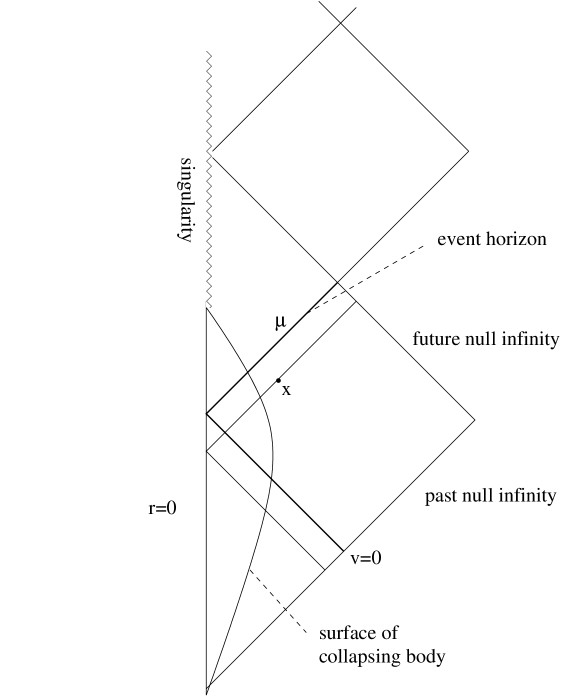
Figure 1: The Penrose diagram of a spherically symmetric collapsing body producing an extremal RN black hole [10]. (The body is shown collapsing to a singularity at $r=0$, but it might instead re-expand into the new asymptotically flat region; see [10] for further discussion of the behavior of charged shells. The behavior of the body after it crosses the event horizon is, of course, not relevant for our analysis.)

2.3 Geometrical optics approximation

To calculate the particle creation rates at late times, we need to propagate the wave packet (20) backward from ${\mycal I}^{+}$ to ${\mycal I}^{-}$. For simplicity, we first investigate the propagation of solution (19); later, the propagation of Eq. (20) can be easily obtained by superposition. A part of the wave (19) will be scattered by the static Schwarzschild field outside the collapsing body and will end up on ${\mycal I}^{-}$ with the same frequency [1] and will not contribute to particle creation. We are interested in the remaining part which will propagate through the center of the collapsing star, eventually emerging to ${\mycal I}^{-}$. Consider the solution (19) propagating to a point $x$, which is very near the future event horizon ${\cal H^{+}}$ and outside the collapsing body (see Fig. 1). The solution near $x$ has a form similar to its form on ${\mycal I}^{+}$,

$$P_{\omega_{0}lm}(x)\sim t(\omega_{0})e^{i\omega_{0}u}Y_{lm}(\theta,\phi),$$ (37)

where $t(\omega_{0})$ is the transmission amplitude describing the fraction of the wave that enters the collapsing body. Note that near the horizon, the effective frequency will be arbitrarily large [9]. So the amplitude of Eq. (37) changes much slower than the phase. Consequently, the geometrical optics approximation becomes valid for the propagation from $x$ back to ${\mycal I}^{-}$. So the wave takes the form

$$P_{\omega_{0}lm}=g(t,r)e^{i\omega_{0}S}Y_{lm}(\theta,\phi),$$ (38)

where $S$ is called the phase of the wave. Each surface of constant $S$ is a null hypersurface [9] and consequently $k^{a}\equiv\nabla^{a}S$ is the tangent to the null geodesics propagating in the radial direction. If we follow a light ray backward in time, it will pass through the center of the star and propagate to ${\mycal I}^{-}$. We fix $(\theta,\phi)$ and consider the family of radial null geodesics $\gamma_{\chi}(\lambda)$ such that for each $\chi$, $\gamma_{\chi}(\lambda)$ represents a null geodesic with parameter $\lambda$ sent from ${\mycal I}^{+}$ radially to the collapsing star. So all geodesics in $\gamma_{\chi}(\lambda)$ have the same path in space but they pass through the center of the star at different times. The limiting null geodesic in this family lies on the future horizon. Set $\chi=0$ for this geodesic and denote it by $\mu$, i.e., $\mu=\gamma_{0}(\lambda)$. Let $x$ be an event lying just outside the horizon (see Fig. 1). According to geometrical optics [9], $S=u(x)$ along a null geodesic. To find out the explicit form of $S$, let $v$ be the Killing/affine parameter coordinate at past null infinity and $v=0$ correspond to the light ray on the horizon. For a fixed collapse, define $v$ on the spacetime by propagation from past null infinity along radial null geodesics. Let $U$ be a smooth Kruskal extension such that it is a constant along each outgoing null geodesic and $U=0$ on the horizon. Therefore, a function $v(U)$ can be constructed from those radial null geodesics with $v(0)=0$. The exact form of $v(U)$ should be solved from the geodesic equation which depends on the details of the collapse. However, no matter what the details of the collapse are, the corresponding spacetime must be smooth. Consequently, the geodesic equation is a smooth equation and thereby $v(U)$ is a smooth function for $U\leq 0$. Equivalently, each smooth Kruskal extension $U$ should correspond to some smooth collapse spacetime for which the propagation of radial null geodesics from future infinity to past null infinity is given by $v=U(u)$. Thus, for the Kruskal extension defined by Eq. (8), we have

$$u=S(v)=-4M\ln(-v)-\frac{2M^{2}}{v}.$$ (39)

There is a close analog between four-dimensional spherical collapse and two-dimensional Minkowski spacetime with a moving mirror. The physical relations have been widely discussed in previous literature, e.g., [6], [7] and [8]. We shall only illustrate the mathematical correspondence between a spherical collapse and a mirror trajectory. In a two-dimensional Minkowski spacetime with double-null coordinates $(u,v)$, a moving mirror servers as boundary of the spacetime. If a left-moving light ray with constant $v$ is reflected by the mirror, it then becomes right-moving with constant $u$. The relation between $u$ and $v$ is uniquely determined by the coordinates, $(u,v)$, of the reflecting point on the mirror. Thus, the mirror trajectory $u=u(v)$ shows how a light ray propagates after reflection. Let the left-moving light ray correspond to an ingoing light ray in a spherical collapse and the right-moving light ray correspond to an outgoing one. Then we see that the mirror plays the role of the origin of spherical coordinates. The trajectory associated with the collapse above is simply Eq. (39). Such a relation will be used later to calculate the energy flux.

The amplitude in Eq. (38) near ${\mycal I}^{-}$ can be calculated by substituting Eq. (38) into $\Box\phi=0$. After neglecting the $\Box g$ term, which is supposed to be small in the geometrical optics approximation, we obtain

$$2k^{a}\nabla_{a}g+g\nabla_{a}k^{a}=0.$$ (40)

Note that $\nabla_{a}k^{a}$ is the expansion of the congruence of radial null geodesics, which is equal to [3]

$$\frac{1}{A}\frac{dA}{d\lambda},$$ (41)

where $\lambda$ is the parameter of $k^{a}$ and $A$ is the cross-sectional area element. Since all geodesics represented by $k^{a}$ point radially and the spacetime is spherically symmetric, $A\propto r^{2}$. Hence, Eq. (40) gives

$$\frac{d\ln(gr)}{d\lambda}=0.$$ (42)

Namely, $gr$ is a constant along each null geodesic. So $gr$ is proportional to $t(\omega_{0})$ in Eq. (37). Finally we get the solution near the past infinity,

$$P_{\omega_{0}lm}\sim\left\{\begin{array}[]{ll}t(\omega_{0})\frac{1}{r}e^{i\omega_{0}S(v)}Y_{lm}(\theta,\phi),&v<0\\ 0,&v>0,\end{array}\right.$$ (45)

where $S(v)$ is given in Eq. (39). Next, superpose solutions the same way as we did on ${\mycal I}^{+}$ (refer to (21)) and assume that $t(\omega)$ varies negligibly over the frequency interval $2\epsilon$. Then, we obtain the wave packet at ${\mycal I}^{-}$,

$$P_{n\epsilon\omega_{0}lm}\sim\left\{\begin{array}[]{ll}t(\omega_{0})\frac{1}{r}z_{p}(v)Y_{lm}(\theta,\phi),&v<0\\ 0,&v>0,\end{array}\right.$$ (48)

where

$$z_{p}(v) \equiv z_{\omega_{0}n}(S(v))$$ (49)

$$= \frac{\sqrt{\epsilon}}{\sqrt{\beta\omega_{0}+\gamma\epsilon}}e^{-i\omega_{0}2n\pi}e^{i\omega_{0}[-4M\ln(-v)-\frac{2M^{2}}{v}]}\hat{f}(\epsilon\tilde{u})$$

and

$$\tilde{u}=-4M\ln(-v)-\frac{2M^{2}}{v}-2n\pi.$$ (50)

2.4 Calculation of particle creation

We shall show that the particle creation rate for each mode with fixed $\omega_{0}$, $\epsilon$, $l$ and $m$ will drop off to zero at sufficiently late times. So in this subsection, we treat $\omega_{0}$ and $\epsilon$ as fixed and consider the limit where $n$ is allowed to become arbitrarily large. The expected number of particles spontaneously created in the state represented by a wave packet is given by [9]

$$N_{n\epsilon}(\omega_{0})=(P^{-},P^{-})_{KG},$$ (51)

where $P^{-}$ represents the negative frequency part of the solution (48). The negative frequency is with respect to $v$. Since the only $v$ dependence in Eq. (48) is $z_{p}(v)$, after integrating on ${\mycal I}^{-}$, (51) reduces to

$$N_{n\epsilon}(\omega_{0})=|t(\omega_{0})|^{2}\int_{0}^{\infty}|\hat{z}(\omega^{\prime})|^{2}\omega^{\prime}d\omega^{\prime},$$ (52)

where

$$\hat{z}(\omega^{\prime}) = \int_{-\infty}^{0}e^{i\omega^{\prime}v}z_{p}(v)dv$$ (53)

$$= \frac{\sqrt{\epsilon}}{\sqrt{\beta\omega_{0}+\gamma\epsilon}}\int_{-\infty}^{0}e^{i\omega^{\prime}v}e^{-i\omega_{0}2n\pi}e^{i\omega_{0}[-4M\ln(-v/\alpha)-\frac{2\alpha M^{2}}{v}]}\hat{f}(\epsilon\tilde{u})dv$$ (54)

is the amplitude of the negative frequency part of $z_{p}(v)$. Note that in $z_{p}(v)$, $v$ is always multiplied by an undetermined factor $1/\alpha$. By a simple rescaling, we see immediately that $N_{n\epsilon}(\omega_{0})$ is independent of the choice of $\alpha$. So without loss of generality, we set $\alpha=1$ from now on. The difficulty in evaluating Eq. (54) is the oscillation in the integrand. We wish to eliminate this oscillation by a Wick rotation. We shall show that the integral in Eq. (54) can be performed along the positive imaginary axis in the complex $v$ plane. To justify the rotation, we need to use the following theorem, which corresponds to one direction of the Paley-Wiener theorem [11].

Theorem 1

Let $f:{\mathrm{I\!R}}\rightarrow{\mathrm{I\!R}}$ be a $C^{\infty}$ function with support in $[-1,1]$. Then, the Fourier transform, $\hat{f}(\zeta)$, of $f$ is an entire analytic function of $\zeta$ such that for all $k>0$,

$$|\hat{f}(\zeta)|\leq\frac{C_{k}e^{|Im\zeta|}}{(1+|\zeta|)^{k}}$$ (55)

for all $\zeta\in{\mbox{\boldmath$C$}}$, where $C_{k}$ is a constant which depends on $k$.

We shall be interested in large $k$. Hence, $k$ is assumed to be large in the rest of the paper. Applying this theorem to $\hat{f}(x)$ defined in (23) with $x$ replaced by $\epsilon\tilde{u}$, we find immediately

$$|\hat{f}(\epsilon\tilde{u})|\leq\frac{C_{k}e^{|Im[\epsilon\tilde{u}]|}}{(1+|\epsilon\tilde{u}|)^{k}}$$ (56)

Thus, in contrast to the integrals considered in [4], the integral appearing in Eq. (54) is convergent. The theorem also tells us that $\hat{f}(\epsilon\tilde{u})$ is an analytic function of $\epsilon\tilde{u}$. Thus, the integrand of Eq. (54) is analytic everywhere in the second quadrant except at the origin of the $v$-plane. However, we can choose a contour which goes around the origin along a circle with infinitesimal radius in the first quadrant. In order to apply Cauchy’s integral theorem, we choose the closed contour as shown in Fig. 2, where $C_{1}$ and $C_{2}$ are two circles with small and large radii, respectively. We are going to show that the integration in Eq. (54) over the two circles is negligible. As for the small circle $C_{1}$, we need to show that the integrand is not divergent in the second quadrant near the origin. From Eqs. (50) and (56), it is easy to see that the only possible source causing the divergence near the origin is $e^{|Im[\epsilon\frac{2\alpha M^{2}}{v}]|}$. However, this term is always suppressed by $e^{-i\frac{2\alpha M^{2}\omega_{0}\omega^{\prime}}{v}}$ in Eq. (49) since $\omega_{0}>\epsilon$. Therefore, the integral over $C_{1}$ approaches zero. To deal with the integration over $C_{2}$, we introduce the following lemma.

Lemma 1

If $F(z)$ satisfies $\lim_{|z|\rightarrow\infty}|F(z)|=0$ in the second quadrant, then
$\int_{C_{2}}e^{icz}F(z)=0$ when the radius of $C_{2}$ approaches infinity, where $c>0$ is a constant.

Figure 2: Integration contour in the $v$-plane

The proof of the lemma is given in the appendix. From Eq. (54) and (56), it is easy to see that the condition of the lemma is satisfied. Therefore, the integration over $C_{2}$ approaches zero. Thus, the integral in Eq. (54) can be performed along the positive imaginary axis in the $v$-plane. Let $x=-i\omega^{\prime}v$. Then the integral in Eq. (54) corresponds to the positive real axis in the $x$-plane,

$$\hat{z}(\omega^{\prime})=\frac{\sqrt{\epsilon}e^{-i\omega_{0}2n\pi}}{-i\omega^{\prime}\sqrt{\beta\omega_{0}+\gamma\epsilon}}\int_{0}^{\infty}e^{-x}e^{-i\omega_{0}4M\ln(\frac{x}{i\omega^{\prime}})}e^{-\frac{2M^{2}\omega_{0}\omega^{\prime}}{x}}\hat{f}(\epsilon\tilde{u}(x))dx,$$ (57)

where

$$\tilde{u}(x)=-4M\ln(\frac{x}{i\omega^{\prime}})+\frac{i2M^{2}\omega^{\prime}}{x}-2n\pi.$$ (58)

Using the fact that $Im[\tilde{u}]=2M\pi+\frac{2M^{2}\omega^{\prime}}{x}$ and $|e^{-i\omega_{0}4M\ln(\frac{x}{i\omega^{\prime}})}|=e^{-2M\pi\omega_{0}}$ when $x$ is real, together with Eq. (57), we have

$$|\hat{z}(\omega^{\prime})| \leq \frac{\sqrt{\epsilon}C_{k}e^{-2M\pi(\omega_{0}-\epsilon)}}{\omega^{\prime}\sqrt{\beta\omega_{0}+\gamma\epsilon}}\int_{0}^{\infty}\frac{e^{-x}e^{-\frac{2M^{2}\omega^{\prime}(\omega_{0}-\epsilon)}{x}}}{(1+|\epsilon\tilde{u}(x)|)^{k}}dx$$ (59)

$$\leq \frac{\sqrt{\epsilon}C_{k}e^{-2M\pi(\omega_{0}-\epsilon)}}{\omega^{\prime}\sqrt{\beta\omega_{0}+\gamma\epsilon}}\int_{0}^{\infty}\frac{e^{-x}e^{-\frac{2M^{2}\omega^{\prime}(\omega_{0}-\epsilon)}{x}}}{|\epsilon\tilde{u}(x)|^{k}}dx.$$ (60)

To proceed, we first derive a lower bound for $|\tilde{u}(x)|$ at large $n$ . Start with

$$|\tilde{u}(x)|^{2}=\left(2n\pi+4M\ln(\frac{x}{\omega^{\prime}})\right)^{2}+\left(2M\pi+\frac{2M^{2}\omega^{\prime}}{x}\right)^{2}.$$ (61)

Let $y=\frac{x}{\omega^{\prime}}$ and define

$$h(y)\equiv|\tilde{u}(x)|^{2}=\left(2n\pi+4M\ln y\right)^{2}+\left(2M\pi+\frac{2M^{2}}{y}\right)^{2}$$ (62)

To find the minimum, we solve $h^{\prime}(y)=0$, which gives

$$-\frac{1}{y^{3}}(8M^{4}+8M^{3}\pi y-16Mn\pi y^{2}-32M^{2}y^{2}\ln y)=0.$$ (63)

Obviously, $y=0$ is not a solution where $h(y)$ achieves its minimum. When $n$ is a large number, the solution to (63) must be at small $y$. So the approximate solution is

$$y_{0}=\frac{M^{3/2}}{\sqrt{n}\sqrt{2\pi}}$$ (64)

and

$$h(y_{0})=(2n\pi)^{2}.$$ (65)

It is easy to check, by computing the second derivative, that $h(y_{0})$ is a minimum for large $n$. So we have an important inequality

$$|\tilde{u}(x)|\geq 2n\pi$$ (66)

for large $n$. Then it follows immediately from Eq. (60) that

$$|\hat{z}(\omega^{\prime})| \leq \frac{\sqrt{\epsilon}C_{k}e^{-2M\pi(\omega_{0}-\epsilon)}}{\omega^{\prime}\sqrt{\beta\omega_{0}+\gamma\epsilon}}\frac{1}{\epsilon^{k}(2n\pi)^{k}}\int_{0}^{\infty}e^{-x}e^{-\frac{2M^{2}\omega^{\prime}(\omega_{0}-\epsilon)}{x}}dx.$$ (67)

However, this bound is not good enough for all $\omega^{\prime}$ since we must integrate $|\hat{z}(\omega^{\prime})|^{2}\omega^{\prime}$ over all $\omega^{\prime}$ and the bound in Eq. (67) will lead to a divergence at small $\omega^{\prime}$. To avoid this divergence, we need to investigate the bound in Eq. (60) more carefully. Denote by $G(\omega^{\prime})$ the integral in Eq. (60), i.e.

$$G(\omega^{\prime})=\int_{0}^{\infty}\frac{e^{-x}e^{-\frac{2M^{2}\omega^{\prime}(\omega_{0}-\epsilon)}{x}}}{|\epsilon\tilde{u}(x)|^{k}}dx.$$ (68)

First, rewrite $|\tilde{u}(x)|^{2}$ in Eq.(61) as

$$|\tilde{u}(x)|^{2}=\left(F_{n}(\omega^{\prime})+4M\ln x\right)^{2}+\left(2M\pi+\frac{2M^{2}\omega^{\prime}}{x}\right)^{2},$$ (69)

where

$$F_{n}(\omega^{\prime})\equiv 2n\pi-4M\ln\omega^{\prime}.$$ (70)

In the following discussion, we choose $\Omega\ll 1$ and consider the frequency range $\omega^{\prime}\leq\Omega$. For $n\gg 1$, $F_{n}(\omega^{\prime})$ is a large positive quantity. Substitute Eq. (69) into Eq. (68)

$$G(\omega^{\prime})=\int_{0}^{\infty}\frac{e^{-x}e^{-\frac{2M^{2}\omega^{\prime}(\omega_{0}-\epsilon)}{x}}}{\epsilon^{k}\left[\left(F_{n}(\omega^{\prime})+4M\ln x\right)^{2}+\left(2M\pi+\frac{2M^{2}\omega^{\prime}}{x}\right)^{2}\right]^{k/2}}dx.$$ (71)

I will evaluate the bound for this integral in three domains of $x$. Choose $a$ such that $a\ll 1$ and $an\gg 1$.

(1)$D1=\{e^{-aF_{n}(\omega^{\prime})/4M}\leq x\leq e^{aF_{n}(\omega^{\prime})/4M}\ and\ x\geq\frac{2M^{2}\omega^{\prime}}{aF_{n}(\omega^{\prime})}\}$
The integral in this interval is approximately

$$G(\omega^{\prime},D1)=\int_{D1}\frac{e^{-x}e^{-\frac{2M^{2}\omega^{\prime}(\omega_{0}-\epsilon)}{x}}}{\epsilon^{k}\left[F_{n}(\omega^{\prime})\right]^{k}}dx.$$ (72)

Since $D1$ is a subset of $(0,\infty)$ and the integrand is always positive, we have

$$G(\omega^{\prime},D1) \leq \frac{1}{\left[\epsilon F_{n}(\omega^{\prime})\right]^{k}}\int_{0}^{\infty}e^{-x}e^{-\frac{2M^{2}\omega^{\prime}(\omega_{0}-\epsilon)}{x}}dx$$ (73)

$$= \frac{2\sqrt{2}}{\left[\epsilon F_{n}(\omega^{\prime})\right]^{k}}\sqrt{M^{2}(\omega_{0}-\epsilon)\omega^{\prime}}K_{1}\left(2\sqrt{2}\sqrt{M^{2}(\omega_{0}-\epsilon)\omega^{\prime}}\right)$$

where $K_{1}$ is a modified Bessel function. For $z\rightarrow 0$, we have $K_{1}(z)\rightarrow\frac{1}{z}$ [12]. Therefore, for small $\omega^{\prime}$, (73) takes the form

$$G(\omega^{\prime},D1)\leq\frac{1}{\left[\epsilon F_{n}(\omega^{\prime})\right]^{k}}.$$ (74)

(2) $D2=\{x\leq\frac{2M^{2}\omega^{\prime}}{aF_{n}(\omega^{\prime})}\}$
The integral in this range is

$$G(\omega^{\prime},D2)=\int_{0}^{\frac{2M^{2}\omega^{\prime}}{aF_{n}(\omega^{\prime})}}\frac{e^{-x}e^{-\frac{2M^{2}\omega^{\prime}(\omega_{0}-\epsilon)}{x}}}{|\epsilon\tilde{u}(x)|^{k}}dx.$$ (75)

Note that $aF_{n}(\omega^{\prime})\leq\frac{2M^{2}\omega^{\prime}}{x}$ gives

$$e^{-\frac{2M^{2}\omega^{\prime}(\omega_{0}-\epsilon)}{x}}\leq e^{-aF_{n}(\omega^{\prime})(\omega_{0}-\epsilon)}.$$ (76)

Replacing $e^{-x}$ by $1$ and using Eqs. (66) and (76) to replace the corresponding terms in the integrand of Eq. (75), we obtain the bound for $G(\omega^{\prime},D2)$,

$$G(\omega^{\prime},D2)\leq\frac{1}{(\epsilon 2n\pi)^{k}}e^{-aF_{n}(\omega^{\prime})(\omega_{0}-\epsilon)}\frac{2M^{2}\omega^{\prime}}{aF_{n}(\omega^{\prime})}.$$ (77)

(3) $D3\equiv\{x\in(0,\infty)|x\notin D1\cup D2\}$
Obviously, $D3$ is a subset of all positive $x$ satisfying $aF_{n}(\omega^{\prime})\leq|4M\ln x|$. Then, it follows from Eq. (68) that

$$G(\omega^{\prime},D3)\leq\int_{0}^{e^{-\frac{aF_{n}(\omega^{\prime})}{4M}}}\frac{e^{-x}e^{-\frac{2M^{2}\omega^{\prime}(\omega_{0}-\epsilon)}{x}}}{|\epsilon\tilde{u}(x)|^{k}}dx+\int_{e^{\frac{aF_{n}(\omega^{\prime})}{4M}}}^{\infty}\frac{e^{-x}e^{-\frac{2M^{2}\omega^{\prime}(\omega_{0}-\epsilon)}{x}}}{|\epsilon\tilde{u}(x)|^{k}}dx.$$ (78)

Replace $|\tilde{u}(x)|$ by $2n\pi$ and $e^{-x}e^{-\frac{2M^{2}\omega^{\prime}(\omega_{0}-\epsilon)}{x}}$ by $1$ in the first integral. Replace $|\tilde{u}(x)|$ by $2n\pi$ and $e^{-\frac{2M^{2}\omega^{\prime}(\omega_{0}-\epsilon)}{x}}$ by $1$ in the second integral. Then we obtain the bound for $G(\omega^{\prime},D3)$

$$G(\omega^{\prime},D3)\leq\frac{1}{(\epsilon 2n\pi)^{k}}e^{-\frac{aF_{n}(\omega^{\prime})}{4M}}+\frac{1}{(\epsilon 2n\pi)^{k}}e^{-e^{\frac{aF_{n}(\omega^{\prime})}{4M}}}.$$ (79)

Combining (74), (77) and (79), we have the bound for $G(\omega^{\prime})$ for $\omega^{\prime}\leq\Omega$, where $\Omega\ll 1$,

$$G(\omega^{\prime}) \leq \frac{1}{\left[\epsilon F_{n}(\omega^{\prime})\right]^{k}}+\frac{1}{(\epsilon 2n\pi)^{k}}e^{-aF_{n}(\omega^{\prime})(\omega_{0}-\epsilon)}\frac{2M^{2}\omega^{\prime}}{aF_{n}(\omega^{\prime})}$$ (80)

$$+ \frac{1}{(\epsilon 2n\pi)^{k}}e^{-\frac{aF_{n}(\omega^{\prime})}{4M}}+\frac{1}{(\epsilon 2n\pi)^{k}}e^{-e^{\frac{aF_{n}(\omega^{\prime})}{4M}}}.$$

Since $F_{n}(\omega^{\prime})$ can be arbitrarily large, we only need to keep the first term on the right-hand-side of Eq. (80). This fact reveals that the integration in Eq. (71) is approximated by taking away the $x$-dependent terms in the denominator of the integrand. Thus, the bound for $|\hat{z}(\omega^{\prime})|$ in (60) at small $\omega^{\prime}$ is

$$|\hat{z}(\omega^{\prime}<\Omega)|\leq\frac{\sqrt{\epsilon}C_{k}e^{-2M\pi(\omega_{0}-\epsilon)}}{\omega^{\prime}\sqrt{\beta\omega_{0}+\gamma\epsilon}}\frac{1}{\left[\epsilon F_{n}(\omega^{\prime})\right]^{k}}.$$ (81)

For $\omega^{\prime}\geq\Omega$, we simply use the bound (67). Then

$$|\hat{z}(\omega^{\prime}>\Omega)|$$ (82)

$$\leq \frac{\sqrt{\epsilon}C_{k}e^{-2M\pi(\omega_{0}-\epsilon)}}{\omega^{\prime}\sqrt{\beta\omega_{0}+\gamma\epsilon}}\frac{2\sqrt{2}}{\epsilon^{k}(2n\pi)^{k}}\sqrt{M^{2}(\omega_{0}-\epsilon)\omega^{\prime}}K_{1}(2\sqrt{2}\sqrt{M^{2}(\omega_{0}-\epsilon)\omega^{\prime}})$$

Now we are ready to compute the particle creation rates at late times. It follows from Eqs. (81) and (82) that Eq. (52) is bounded by

$$N_{n\epsilon}(\omega_{0}) \leq |t(\omega_{0})|^{2}\frac{\epsilon C_{k}^{2}e^{-4M\pi\omega_{0}}}{(\beta\omega_{0}+\gamma\epsilon)\epsilon^{2k}}\left[\int_{0}^{\Omega}\frac{1}{\omega^{\prime}}\frac{1}{(2n\pi-4M\ln\omega^{\prime})^{2k}}d\omega^{\prime}\right.$$ (83)

$$+ \left.\frac{8}{n^{2k}}\int_{\Omega}^{\infty}\frac{M^{2}(\omega_{0}-\epsilon)}{\omega^{\prime}}K_{1}^{2}(2\sqrt{2}\sqrt{M^{2}(\omega_{0}-\epsilon)\omega^{\prime}})d\omega^{\prime}\right].$$

Evaluating the first integral gives

$$\frac{4M}{(2k-1)}\frac{1}{(2n\pi-4M\ln\Omega)^{2k-1}}\approx\frac{4M}{(2k-1)}\frac{1}{(2n\pi)^{2k-1}}$$

The second integral in Eq. (83) is convergent since $K_{1}(z)\sim\sqrt{\frac{\pi}{2z}}e^{-z}$ for large $|z|$ [12]. Since $n$ represents time, we conclude that the particle creation rate for any mode decays with time faster than any power law. Furthermore, by summing over $n$ from any positive integer to infinity, the bound in Eq. (83) is still finite. This means that, as mentioned in the introduction, the accumulation of particles after an infinite time is finite. This conclusion is derived from a particular Kruskal transformation (8), which corresponds to a particular process of collapse. A different process of collapse will give rise to a different Kruskal coordinate $U^{\prime}$, which is a smooth function of $U$. We conjecture that our conclusion that the particle creation rate decays with time faster than any power law is independent of the choice of the Kruskal extension, i.e., independent of the details of collapse. As evidence in this conjecture, one can check, following similar steps, that the smooth extension (32) also gives the same result.

3 Stress energy tensor

In two-dimensional Minkowski spacetime, the renormalized energy flux in a spacetime with a moving mirror boundary in the “in” vacuum state is [8]

$$<T_{uu}>_{q}=\frac{1}{4\pi}\left[\frac{1}{4}\left(\frac{p^{\prime\prime}}{p^{\prime}}\right)^{2}-\frac{1}{6}\frac{p^{\prime\prime\prime}}{p^{\prime}}\right],$$ (84)

where $p=v=p(u)$ is the trajectory of the mirror. According to the discussion in the last section, $p$ is exactly a Kruskal extension $U$ which describes a particular collapse. The corresponding trajectory of Kruskal extension (8) is thereby

$$u=-4M\ln(-p)-\frac{2M^{2}}{p}.$$ (85)

Straightforward calculation yields

$$<T_{uu}>=\frac{p^{3}(p-2M)}{48\pi M^{2}(M-2p)^{4}},$$ (86)

which approaches

$$<T_{uu}>\sim\frac{1}{u^{3}}$$ (87)

for large $u$. Therefore, $<T_{uu}>$ decays as $1/u^{3}$.

The quantity $<T_{uu}>$ can be estimated from the particle flux by adding up all frequency modes at certain time

$$<T_{uu}>\sim\int_{0}^{\infty}N_{n\epsilon}(\omega_{0})\omega_{0}d\omega_{0}.$$ (88)

This formula, as discussed in [8], is a naive energy-particle relation. It is correct only when particles emitted in different modes are not correlated. However, it is worth comparing this naive $<T_{uu}>$ with the one in Eq. (87). If the naive one is smaller, it may indicate some serious problems in our calculation of $N_{n\epsilon}(\omega_{0})$. From the estimation of $N_{n\epsilon}(\omega_{0})$ in the last section, Eq. (88) suggests that the naive $<T_{uu}>$ also should decay to zero faster than any inverse power of $u$. So the result (87) may seem to be inconsistent with the particle creation results. However, in the last section, we treated $\omega_{0}$ and $\epsilon$ as fixed while allowing $n$ to be arbitrarily large. But Eq. (88) requires us to sum over all modes at a fixed time $n$. So we need to reevaluate the bound of $N_{n\epsilon}$ for arbitrarily small $\omega_{0}$. In this subsection, we focus on the (1+1)-dimensional RN black hole formed by collapse because our purpose is to check the consistency of (87) which is computed in a 1+1-dimensional spacetime. The calculation will be parallel to our four dimensional case in the previous sections. One important difference is that the transmission amplitude $t(\omega_{0})$ has unit magnitude due to the fact that a (1+1)-spacetime is conformal to Minkowski spacetime and therefore the outgoing wave packet will not be scattered when it is propagated backward in time. So the bound in Eq. (83) still holds for the (1+1)-dimensional case except $|t(\omega_{0})|=1$. However, for our present purposes, the bound in Eq. (60) becomes inappropriate since $|\epsilon\tilde{u}(x)|\gg 1$ is not always true for arbitrarily small $\epsilon$. So we stick to Eq. (59) and follow similar arguments. Denote by $H(\omega^{\prime})$ the integral in (68), i.e.,

$$H(\omega^{\prime})=\int_{0}^{\infty}\frac{e^{-x}e^{-\frac{2M^{2}\omega^{\prime}(\omega_{0}-\epsilon)}{x}}}{(1+|\epsilon\tilde{u}(x)|)^{k}}dx.$$ (89)

Consequently, the corresponding changes in Eq. (80) become

$$H(\omega^{\prime}) \leq \frac{1}{\left[1+\epsilon F_{n}(\omega^{\prime})\right]^{k}}+\frac{1}{(1+\epsilon 2n\pi)^{k}}e^{-aF_{n}(\omega^{\prime})(\omega_{0}-\epsilon)}\frac{2M^{2}\omega^{\prime}}{aF_{n}(\omega^{\prime})}$$

$$+ \frac{1}{(1+\epsilon 2n\pi)^{k}}e^{-\frac{aF_{n}(\omega^{\prime})}{4M}}+\frac{1}{(1+\epsilon 2n\pi)^{k}}e^{-e^{\frac{aF_{n}(\omega^{\prime})}{4M}}}.$$

The last two terms in the bound are still negligible due to the exponentials. Unlike before, we are not certain whether the second term is much smaller than the first term since $\omega_{0}-\epsilon$ can be arbitrarily small now. So we keep both of the terms. In order to perform integrals easily, we replace the exponential and $\omega^{\prime}$ in the numerator by $1$ in the second term. Thus,

$$H(\omega^{\prime}) \leq \frac{1}{\left[1+\epsilon F_{n}(\omega^{\prime})\right]^{k}}+\frac{1}{(1+\epsilon 2n\pi)^{k}}\frac{2M^{2}}{aF_{n}(\omega^{\prime})}$$ (91)

Then (59) becomes

$$|\hat{z}(\omega^{\prime}<\Omega)| \leq \frac{\sqrt{\epsilon}C_{k}e^{-2M\pi(\omega_{0}-\epsilon)}}{\omega^{\prime}\sqrt{\beta\omega_{0}+\gamma\epsilon}}\left(\frac{1}{\left[1+\epsilon F_{n}(\omega^{\prime})\right]^{k}}+\frac{1}{(1+\epsilon 2n\pi)^{k}}\frac{2M^{2}}{aF_{n}(\omega^{\prime})}\right).$$ (92)

The modification for $\hat{z}(\omega^{\prime}>\Omega)$ in Eq. (82) is

$$|\hat{z}(\omega^{\prime}>\Omega)|$$ (93)

$$\leq \frac{\sqrt{\epsilon}C_{k}e^{-2M\pi(\omega_{0}-\epsilon)}}{\omega^{\prime}\sqrt{\beta\omega_{0}+\gamma\epsilon}}\frac{2\sqrt{2}}{(1+\epsilon 2n\pi)^{k}}\sqrt{M^{2}(\omega_{0}-\epsilon)\omega^{\prime}}K_{1}\left(2\sqrt{2}\sqrt{M^{2}(\omega_{0}-\epsilon)\omega^{\prime}}\right)$$

Thus, the bound on the particle number from (52) is

$$N_{n\epsilon}(\omega_{0})$$

$$\leq \frac{2\epsilon C_{k}^{2}e^{-4M\pi(\omega_{0}-\epsilon)}}{\beta\omega_{0}+\gamma\epsilon}\int_{0}^{\Omega}\frac{1}{\omega^{\prime}}\left(\frac{1}{\left[1+\epsilon F_{n}(\omega^{\prime})\right]^{k}}\right)^{2}+\frac{1}{\omega^{\prime}}\left(\frac{1}{(1+\epsilon 2n\pi)^{k}}\frac{2M^{2}}{aF_{n}(\omega^{\prime})}\right)^{2}d\omega^{\prime}$$

$$+ \frac{\epsilon C_{k}^{2}e^{-4M\pi(\omega_{0}-\epsilon)}}{\beta\omega_{0}+\gamma\epsilon}\frac{8}{(1+\epsilon 2n\pi)^{2k}}\int_{\Omega}^{\infty}\frac{M^{2}(\omega_{0}-\epsilon)\omega^{\prime}}{\omega^{\prime}}K_{1}^{2}\left(2\sqrt{2}\sqrt{M^{2}(\omega_{0}-\epsilon)\omega^{\prime}}\right)d\omega^{\prime},$$

where we have used the inequality $(A+B)^{2}\leq 2(A^{2}+B^{2})$. The integration over $(0,\Omega)$ gives

$$\frac{2\epsilon C_{k}^{2}e^{-4M\pi(\omega_{0}-\epsilon)}}{\beta\omega_{0}+\gamma\epsilon}\left(\frac{1}{(2k-1)4M\epsilon}\frac{1}{(1+2n\pi\epsilon)^{2k-1}}+\frac{M^{3}}{2n\pi a^{2}(1+2n\pi\epsilon)^{2k}}\right),$$ (95)

where we have neglected the $\Omega$-dependent term since it is small compared with $n$. To estimate the integration over $(\Omega,\infty)$, we first change the integration variable from $\omega^{\prime}$ to $x=(\omega_{0}-\epsilon)\omega^{\prime}$. Thus the integral becomes $M^{2}\int_{\Omega(\omega_{0}-\epsilon)}^{\infty}K_{1}^{2}\left(2\sqrt{2}\sqrt{M^{2}x}\right)dx$. We then split the integral into two terms as

$$M^{2}\int_{\Omega(\omega_{0}-\epsilon)}^{b}K_{1}^{2}\left(2\sqrt{2}\sqrt{M^{2}x}\right)dx+M^{2}\int_{b}^{\infty}K_{1}^{2}\left(2\sqrt{2}\sqrt{M^{2}x}\right)dx,$$ (96)

where $b>\Omega(\omega_{0}-\epsilon)$ and $bM^{2}\ll 1$. Thus, we can use the approximate form of $K_{1}(z)\sim 1/z$ again for the first term. The second term is just a constant and negligible compared to the first term when $\omega_{0}$ is taken small enough. Therefore, the integral is approximately $\frac{-M^{2}}{2\sqrt{2}}\ln[\Omega(\omega_{0}-\epsilon)]$. Together with a coefficient, the second integral in Eq. (LABEL:nnp) yields

$$\frac{\epsilon C_{k}^{2}e^{-2M\pi\omega_{0}}}{\beta\omega_{0}+\gamma\epsilon}\frac{8}{(1+\epsilon 2n\pi)^{2k}}\frac{-M^{2}}{2\sqrt{2}}\ln[\Omega(\omega_{0}-\epsilon)].$$ (97)

As discussed above, the main contribution to $<T_{uu}>$ comes from the low-frequency integration $\int_{0}^{\delta}N(\omega_{0})\omega_{0}d\omega_{0}$, where $\delta$ is a small constant. Since it is assumed $\epsilon<\omega_{0}$, we can no longer treat $\epsilon$ as constant when performing the integral. For convenience, we choose $\epsilon$ to be a small fraction of $\omega_{0}$. It follows from Eqs. (95) and (97) that

$$\int_{0}^{\delta}N_{n\epsilon}(\omega_{0})\omega_{0}d\omega_{0}\leq\frac{K}{n},$$ (98)

where $K$ is a constant. Thus, although the particle creation rate in each individual mode goes to zero faster than any inverse power of time, the energy flux estimated from the particle creation rate decays only as $1/u$ on account of contributions from the very low frequency modes. The bound in Eq. (98) decays more slowly with time than Eq. (87). This difference may be due to the fact that the bound (98) is not sharp enough. An alternative possible explanation is that, as pointed out by Davies and Fulling [8], the relationship between particle fluxes and energy fluxes can be more subtle than (88) as a result of destructive interference between different modes. At this stage, we do not know if there exists interference since we only have the upper bound on the number of particles.

One can also ask if the $1/u^{3}$ decay rate of energy flux is independent of the details of the collapse. Since each collapse corresponds to a smooth extension, let us consider another smooth extension $q$ and the function $q=q(u)$, which gives the related energy flux,

$$<T_{uu}>_{q}=\frac{1}{4\pi}\left[\frac{1}{4}\left(\frac{q^{\prime\prime}}{q^{\prime}}\right)^{2}-\frac{1}{6}\frac{q^{\prime\prime\prime}}{q^{\prime}}\right].$$ (99)

Let $q=g(p)$. From $q(u)=g(p(u))$, we derive the relationship between $<T_{uu}>_{q}$ and $<T_{uu}>_{p}$ (the energy flux associated with $p$),

$$<T_{uu}>_{q}=<T_{uu}>_{p}+[p^{\prime}(u)]^{2}\frac{3g^{\prime\prime}(p)^{2}-2g^{\prime}(p)g^{\prime\prime\prime}(p)}{48\pi g^{\prime}(p)^{2}}.$$ (100)

Since $p$ and $q$ are two smooth coordinates, the derivatives of $g(p)$ must be finite and $g^{\prime}(p)\neq 0$. From Eq. (85), $[p^{\prime}(u)]^{2}$ goes as $1/u^{4}$ at late times. Therefore, the second term on the right-hand side of (100) is negligible compared to the first term which goes as $1/u^{3}$. Therefore, we showed that the $1/u^{3}$ decay rate is invariant under a smooth change of mirror trajectory. This fact agrees with the fact that the late-time radiation is independent of the details of collapse. If one applies the extension (10) to compute the energy flux, as done in [4], the energy flux would be identical zero at late times. This is because the extension (10) fails to be a smooth one (see the comment at the end of section 2.2) at late times (around $U=0$).

4 Conclusions

We have calculated the number of particles created from a massless scalar field on an extremal RN black hole spacetime formed by collapse. We found that for each mode associated with a wave packet, the rate of particle creation drops off to zero faster than any inverse power of time at late times. Consequently, even after an infinite time, the number of particles detected by a detector sensitive to a certain frequency is finite. This result confirms that extremal black holes do not create particles. In the (1+1)-dimensional case, the stress-energy flux falls off as $1/u^{3}$. This result is not in contradiction with the much more rapid decay of each mode, since the very low frequency modes do not achieve their asymptotic decay rate until very late times.

Acknowledgments

It is my pleasure to express my thanks to professor Robert M. Wald for many helpful discussions on this project.

This research was supported by NSF grants/PHY00-90138 to the University of Chicago. This work was also supported in part by a grant, through CENTRA, from FCT (Portugal).

Appendix: Proof of Lemma 1

Let $R$ denote the radius of $C_{2}$ and $I_{R}\equiv\int_{C_{2}}e^{icz}F(z)$. Substitute $z$ by $Re^{i\theta}$. Then

$$I_{R}=\int_{\frac{\pi}{2}}^{\frac{3\pi}{2}}e^{icR\cos\theta-cR\sin\theta}F(Re^{i\theta})iRe^{i\theta}d\theta.$$ (101)

Since $\lim_{|z|\rightarrow\infty}|F(z)|\rightarrow 0$, for any $\epsilon^{\prime}>0$, we can find $R$ such that

$$|I_{R}| \leq \epsilon^{\prime}R\int_{\frac{\pi}{2}}^{\frac{3\pi}{2}}e^{-cR\sin\theta}d\theta$$ (102)

$$\leq \epsilon^{\prime}R\int_{0}^{\frac{\pi}{2}}e^{-cR\cos\theta}d\theta.$$

In the range $[0,\frac{\pi}{2}]$,

$$\cos\theta\geq 1-\frac{2}{\pi}\theta$$

Therefore,

$$|I_{R}| \leq \epsilon^{\prime}R\int_{0}^{\frac{\pi}{2}}e^{-cR(1-\frac{2}{\pi}\theta)}d\theta$$

$$\leq \frac{\pi}{2c}\epsilon^{\prime}(1-e^{-cR}).$$

Therefore,

$$\lim_{R\rightarrow\infty}|I_{R}|=0.$$ (103)

References

• [1] S. W. Hawking, Commun. math. Phys. 43, 199-220 (1975)
• [2] R. M. Wald, Commun. math. Phys. 45, 9-34 (1975)
• [3] R. M. Wald, Quantum Field Theory in Curved Spacetime and Black Hole Thermodynamics (University of Chicago, 1994)
• [4] S. Liberati, T. Rothman, S. Sonego, Phys. Rev. D 62, 024005 (2000)
• [5] K. Lake, Phys. Rev. D 20, 370 (1979)
• [6] N. D. Birrell and P. C. W. Davies, Quantum fields in curved space (Cambridge University Press, Cambridge, England, 1982).
• [7] S. A. Fulling and P.C. W. Davies, Proc. R. Soc. Lond. A. 348, 393-414 (1976)
• [8] P. C. W. Davies and S. A. Fulling, Proc. R. Soc. Lond. A. 356, 237-257 (1977)
• [9] R. M. Wald, General Relativity (University of Chicago Press, Chicago, 1984)
• [10] D. G. Boulware, Phys. Rev. D, 8,2363 (1973)
• [11] M. Reed and B. Simon, Methods of Modern Mathematical Physics II: Fourier Analysis, Self-Adjointness (Academic Press, New York, 1975)
• [12] M. Abramowitz and I. A. Stegun, Handbook of Mathematical Functions (Dover, New York, 1972)