Qualitative Analysis of Universes with Varying Alpha

Abstract

Assuming a Friedmann universe which evolves with a power-law scale factor, $a=t^{n}$, we analyse the phase space of the system of equations that describes a time-varying fine structure ’constant’, $\alpha$, in the Bekenstein-Sandvik-Barrow-Magueijo generalisation of general relativity. We have classified all the possible behaviours of $\alpha(t)$ in ever-expanding universes with different $n$ and find new exact solutions for $\alpha(t)$. We find the attractors points in the phase space for all $n$. In general, $\alpha$ will be a non-decreasing function of time that increases logarithmically in time during a period when the expansion is dust dominated ($n=2/3$), but becomes constant when $n>2/3$. This includes the case of negative-curvature domination ($n=1$). $\alpha$ also tends rapidly to a constant when the expansion scale factor increases exponentially. A general set of conditions is established for $\alpha$ to become asymptotically constant at late times in an expanding universe.

1 Introduction

Stimulated by the observations for small variations in atomic structure controlled by the fine structure constant in quasar absorption lines at redshifts $z=1-3$, [1, 2, 3], there has been much recent interest in the theoretical predictions of gravity theories which extend general relativity to incorporate space-time variations of the fine structure ’constant’. These have been primary formulated as Lagrangian theories with explicit variation of the velocity of light, $c$, [4, 5, 6], or of the charge on the electron, $e,$ [10, 9, 8, 7]. Theories of the latter sort offer the possibility of matching the magnitude and trend of the quasar observations and have been studied numerically and by means of matched asymptotic approximations. They are also of particular interest because they predict that violations of the weak equivalence principle should be observed at a level that is within about an order of magnitude of existing experimental bounds [11, 12, 13]. They are consistent with all other astrophysical and experimental limits of time variation of the fine structure constant and predict effects of the microwave background radiation, primordial nucleosynthesis, and the Oklo natural reactor that are too small to conflict with current observational bounds. A range of variant theories have been investigated with attention to the possible particle physics motivations and consequences for systems of grand and partial unification in references [14, 15, 16]. In this paper we will give a full qualitative analysis of the properties of Friedmann cosmological models in a sub-class of these theories developed initially by Bekenstein [17] to generalise Maxwell’s equations to include varying $e$ and then generalised by Sandvik, Barrow and Magueijo [10] to include gravitation. We refer to these as BSBM theories. We provide a phase-space analysis of the non-linear propagation equation for the scalar field which carries the variations of the fine structure constant. Some new exact solutions are also given and all the asymptotic behaviours classified.

2 The BSBM Theory

2.1 The Cosmological Evolution Equations

We will assume that the total action of the Universe is given by BSBM:

$$S=\int d^{4}x\sqrt{-g}\left(\mathcal{L}_{grav}+\mathcal{L}_{matter}+\mathcal{L}_{\psi}+\mathcal{L}_{em}e^{-2\psi}\right),$$ (1)

In the BSBM varying $\alpha$ theory, the quantities $c$ and $\hbar$ are taken to be constant, while $e$ varies as a function of a real scalar field $\psi,$ with

$$e=e_{0}e^{\psi}$$ (2)

where $\mathcal{L}_{\psi}={\frac{\omega}{2}}\partial_{\mu}\psi\partial^{\mu}\psi$, $\omega$ is a coupling constant, and $\mathcal{L}_{em}=-\frac{1}{4}f_{\mu\nu}f^{\mu\nu}$. The gravitational Lagrangian is the usual $\mathcal{L}_{g}=-\frac{1}{16\pi G}R$, with $R$ the curvature scalar and we have defined an auxiliary gauge potential $a_{\mu}=\epsilon A_{\mu},$ and field tensor $f_{\mu\nu}=\epsilon F_{\mu\nu}=\partial_{\mu}a_{\nu}-\partial_{\nu}a_{\mu}$, so the covariant derivative takes the usual form, $D_{\mu}=\partial_{\mu}+ie_{0}a_{\mu}$. The dependence on $\epsilon$ in the Lagrangian then occurs only in the kinetic term for $\epsilon$ and in the $F^{2}=f^{2}/\epsilon^{2}$ term.

The universe will be described by a homogeneous and isotropic Friedmann metric with expansion scale factor $a(t)$ and curvature parameter $k.$ Varying the total Lagrangian we obtain the Friedmann equation ($G=c\equiv 1$) for a universe containing pressure-free matter and radiation:

$$\left(\frac{\dot{a}}{a}\right)^{2}=\frac{8\pi}{3}\left(\rho_{m}\left(1+\left|\zeta\right|e^{-2\psi}\right)+\rho_{r}e^{-2\psi}+\rho_{\psi}+\rho_{\Lambda}\right)-\frac{k}{a^{2}}$$ (3)

where the cosmological vacuum energy $\rho_{\Lambda}$ is a constant given by $\Lambda/(8\pi)$, and $\rho_{\psi}=\frac{\omega}{2}\dot{\psi}^{2}$ and $\zeta=\mathcal{L}_{em}/\rho_{m}$ is the fraction of the matter which carries electric or magnetic charge.

For the scalar field we obtain the evolution equation

$$\ddot{\psi}+3H\dot{\psi}=-\frac{2}{\omega}\exp[-2\psi]\zeta\rho_{m}$$ (4)

where $H\equiv\dot{a}/a$ is the Hubble parameter. The conservation equations for the non-interacting radiation and matter densities, $\rho_{r}$ and $\rho_{m}$ respectively, are:

$$\dot{\rho_{m}}+3H\rho_{m} = 0$$ (5)

$$\dot{\rho}_{r}+4H\rho_{r} = 2\dot{\psi}\rho_{r}.$$ (6)

so $\rho_{m}\propto a^{-3}$. However, the last relation can be written as $\dot{\tilde{\rho}_{r}}+4H\tilde{\rho}_{r}=0,$ with $\tilde{\rho}_{r}\equiv\rho_{r}e^{-2\psi}\propto a^{-4}$.

The Friedmann models with varying $\alpha$ have been shown [9] to have the property that when $\zeta<0$ the homogeneous motion of the $\psi$ does not create significant metric perturbations at late times. This means that far from the singularity we can safely assume that the expansion scale factor follows the form for the Friedmann universe containing the same fluid when $\alpha$ does not vary $(\zeta=0=\psi)$. The behaviour of $\psi$ then follows from a solution of equation (4) in which $a(t)$ has the form for a Friedmann universe for matter with the same equation of state in general relativity when $\zeta=0=\psi.$ This behaviour is natural. We would not expect that very small variations in the coupling to electromagnetically interacting matter would have large gravitational effects upon the expansion of the universe. Thus, in this paper we will provide a complete analysis of the behaviour of the solutions of the non-linear propagation equation (4) for appropriate behaviours of $a(t).$

2.2 An Approximation Method

We consider spatially flat universes ($k=0$) and assume that the expansion scale factor is that of the Friedmann model containing a perfect fluid:

$$a=t^{n}$$ (7)

where $n$ is a constant. The late stages of an open universe containing fluid with density $\rho$ and pressure $p$ obeying $\rho+3p>0$ can be studied by considering the case $n=1.$ We rewrite the wave equation (4) as

$$\ (\dot{\psi}a^{3}\dot{)}=-\frac{2\zeta}{\omega}\rho_{m}a^{3}\exp[-2\psi]$$

Therefore, since $\rho_{m}a^{3}$ is constant this reduces to a Liouville equation of the form

$$(\dot{\psi}a^{3})^{.}=\ N\exp[-2\psi]$$ (8)

where $N$ is a constant, defined by

$$N\equiv-\frac{2\zeta}{\omega}\rho_{m}a^{3}\ .$$ (9)

We shall consider first the cosmological models that arise when the defining constant $N$ is negative. This arises when the constant $\zeta<0,$ indicating that the matter content of the universe is dominated by magnetic rather than electrostatic energy. The value of $\zeta$ for baryonic and dark matter has been disputed [12, 16, 10]. It is the difference between the percentage of mass in electrostatic and magnetostatic forms. As explained in [10], we can at most estimate this quantity for neutrons and protons, with $\zeta_{n}\approx\zeta_{p}\sim 10^{-4}$. We may expect that for baryonic matter $\zeta\sim 10^{-4}$, with composition-dependent variations of the same order. The value of $\zeta$ for the dark matter, for all we know, could be anything between -1 and 1. Superconducting cosmic strings, or magnetic monopoles, display a negative $\zeta$, unlike more conventional dark matter. It is clear that the only way to obtain a cosmologically increasing $\alpha$ in BSBM is with $\zeta<0$, i.e with unusual dark matter, in which magnetic energy dominates over electrostatic energy. In [10] we showed that fitting the Webb et al results requires $\zeta/\omega=-2\pm 1\times 10^{-4}$, where $\zeta$ is weighted by the necessary fractions of dark and baryonic matter required by observations of the gravitational effects of dark matter and the calculations of Big Bang nucleosynthesis. We note also that in practice $\zeta$ might display a significant spatial variation because of the change in the nature of the dominant form of dark matter over different length scales. For example, a magnetically dominated form of dark matter might contribute a negative value of $\zeta$ on large scales while domination of the matter content by baryons on small scales would lead to $\zeta>0$ locally. We will not discuss the effects of such variations in this paper.

2.3 The Validity of the Approximation

We have assumed that the scale factor is given by the FRW model and then solved the $\psi$ evolution equation. This is a good approximation up to logarithmic corrections. Here is what happens to higher order.

We take the leading order behaviour in (3)

$$\left(\frac{\dot{a}}{a}\right)^{2}\approx\frac{8\pi}{3}\rho_{m}\left(1+\left|\zeta\right|e^{-2\psi}\right)$$ (10)

Now if we take $a=t^{2/3}$ so

$$\frac{8\pi}{3}\rho_{m}=\frac{4}{9t^{2}}$$

and solve equation (8) we get asymptotically,

$$\psi=\frac{1}{2}\ln[2N\ln t]\rightarrow\ln[\ln t]$$ (11)

to leading order at late times. Suppose we now re-solve (10) with the $\left|\zeta\right|e^{-2\psi}$ correction included

$$\left(\frac{\dot{a}}{a}\right)^{2}\approx\frac{4}{9t^{2}}\ \left(1+\left|\zeta\right|e^{-2\psi}\right)\approx\frac{4}{9t^{2}}\left(1+\frac{\left|\zeta\right|}{\ \ln t}\right)$$ (12)

Note that the kinetic term which we neglected is of order

$$\omega\dot{\psi}^{2}\sim\frac{1}{4t^{2}\ln^{2}t}$$ (13)

and so is smaller than the term we have retained. Solving equation (10) we have

$$\ln a=\frac{2\left|\zeta\right|}{3}\left[sh^{-1}\left\{\sqrt{\frac{\ln t}{\left|\zeta\right|}}\right\}+\sqrt{\frac{\ln t}{\left|\zeta\right|}}\sqrt{1+\frac{\ln t}{\left|\zeta\right|}}\right]$$ (14)

Note that when $\left|\zeta\right|\rightarrow 0$ this gives the usual $\ln a=\frac{2}{3}\ln t$. When $\left|\zeta\right|\neq 0$ we have

$$\ln a\rightarrow\frac{2\left|\zeta\right|}{3}\left\{\ln[2\sqrt{\frac{\ln t}{\left|\zeta\right|}}]+\frac{\ln t}{\left|\zeta\right|}\right\}$$

and

$$a=t^{2/3}(\ln t)^{\left|\zeta\right|/3}$$ (15)

where $\left|\zeta\right|$ is small and so the corrections to the $a=t^{2/3}$ ansatz are small. In terms of the Hubble rate:

$$H=\frac{2}{3t}+\frac{\left|\zeta\right|}{3t\ln t}$$

If we include the kinetic corrections to equation (10) then as $\dot{\psi}=\frac{1}{2t\ln t}$

$$\left(\frac{\dot{a}}{a}\right)^{2}\approx\frac{4}{9t^{2}}\ \left(1+\left|\zeta\right|e^{-2\psi}\ \right)+\frac{4\pi\omega}{3}\dot{\psi}^{2}\approx\frac{4}{9t^{2}}\left(1+\frac{\left|\zeta\right|}{\ \ln t}+\frac{S}{\ \ln^{2}t}\right)$$ (16)

where

$$S\equiv\frac{3\pi\omega}{4}$$

So, if $x=\ln t,$we have

$$\frac{3}{2}\ln a = \sqrt{x^{2}+\left|\zeta\right|x+S}+S\int\frac{dx}{x\sqrt{x^{2}+\left|\zeta\right|x+S}}$$ (17)

$$+\frac{\left|\zeta\right|}{2}\int\frac{dx}{\sqrt{x^{2}+\left|\zeta\right|x+S}}$$

$$\frac{3}{2}\ln a = \sqrt{x^{2}+\left|\zeta\right|x+S}-\ln\left[\frac{2S+\left|\zeta\right|x+2\sqrt{S}\sqrt{x^{2}+\left|\zeta\right|x+S}}{x}\right]$$ (18)

$$+\frac{\left|\zeta\right|}{2}\ln\left[2\sqrt{x^{2}+\left|\zeta\right|x+S}+2x+\left|\zeta\right|\right]$$

Again, as $t\rightarrow\infty$ the leading order behaviour is that found in equation (15).

In the radiation era we have an exact solution of equation (8) with

$$2\psi=\ln(8N)+\frac{1}{2}\ln t$$ (19)

so the corrections to the Friedmann equation look like

$$\left(\frac{\dot{a}}{a}\right)^{2}\approx\frac{1}{4t^{2}}\ \left(1+\left|\zeta\right|e^{-2\psi}\right)\approx\frac{1}{4t^{2}}\left(1+\frac{\left|\zeta\right|}{8N\ t^{1/2}}\right)$$ (20)

and these corrections fall off much faster than in the dust case. Again, our basic approximation method holds good to high accuracy.

2.4 A Linearisation Instability

Despite the robustness of the basic test-motion approximation that we are employing to analyse the evolution of $\psi(t)$ as the universe expands, there is a subtle feature the non-linear evolution equation (8) which must be noted in order that spurious conclusions are not drawn from an approximate analysis. We see that the right-hand side of equation (8) is always positive. Therefore $\psi$ can never experience an expansion maximum (where $\dot{\psi}=0$ and $\ddot{\psi}<0$) and therefore $\psi(t)$ can never oscillate. However, if we were to linearise equation (8), obtaining

$$(\dot{\psi}a^{3})^{.}=\ N\exp[-2\psi]\approx N(1-2\psi+O(\psi^{2}))$$

then for $\psi>1/2$ the right-hand side takes negative values and pseudo-oscillatory solutions for $\psi$ would appear that are not the linearised approximation to any true solution of the non-linear equation (8). Care must therefore be taken to ensure that analytic approximations are not extended to large $\psi$ and that numerical analyses are not creating spurious spirals in the phase plane by virtue of a linearisation procedure; for a fuller discussion see ref. [7].

These considerations can be taken further. It is possible for $\psi(t)$ to decrease, reach a minimum and then increase. But it is not possible for $\psi(t)$ to decrease if it has ever increased. A second interesting consequence of this feature of equation (8) is that it holds true even if $a(t)$ reaches an expansion maximum and begins to contract. Thus in a closed universe we expect $\psi$ and $\alpha$ to continue to increase slowly even after the universe begins to contract. This will have important consequences for the expected variation of $\psi$ and $\alpha$ in realistically inhomogeneous universes.

3 Phase-plane Analysis

3.1 A transformation of variables

In this section we will look at the $\psi$ equation of motion (8)when the expansion scale factor takes the power-law form (7). The evolution equation for the field then becomes:

$$\frac{d}{dt}\left(\dot{\psi}t^{3n}\right)=N\exp[-2\psi]$$ (21)

with $N>0.$ We introduce the following variables :

$$x=ln(t)\qquad y=\psi-Ax-B\qquad A=1-\frac{3n}{2}\qquad B=\frac{1}{2}\ln(N)$$ (22)

and rewrite (8) as:

$$y^{\prime\prime}+(3n-1)(y^{\prime}+1-\frac{3n}{2})=e^{-2y},$$ (23)

where ^′ $\equiv d/dx$. This second-order differential equation can be transformed into an autonomous system by defining $v=\frac{dy}{dx}$ and $u=y$:

$$\frac{dv}{dx} = e^{-2u}+(1-3n)(v+1-\frac{3n}{2})$$ (24)

$$\frac{du}{dx} = v$$

We see that the system has a finite critical point at

$$(u_{c},v_{c})=(-\frac{1}{2}\ln{[(1-3n)(\frac{3n}{2}-1)]},0)$$ (25)

when $n\in(\frac{1}{3},\frac{2}{3})$ and it has a infinite critical point at $(u_{c},v_{c})=(+\infty,0)$ when $n=\frac{1}{3}$ or $n=\frac{2}{3}$. The finite critical points correspond to the family of exact solutions of the form $\psi=B+A\ln(t)$ found in [9]. In the original variables these solutions are

$$\psi=\frac{1}{2}\ln[\frac{2N}{(2-3n)(3n-1)}]+\left(\frac{2-3n}{2}\right)\ln(t).$$

In order to analyse the system fully, we will study finite critical points and the critical points at infinity separately. We will also distinguish several domains of behaviour for $n$: $n=\frac{1}{3}$, $n=\frac{2}{3}$, $n\in(\frac{1}{3},\frac{2}{3})$, $n<\frac{1}{3}$ and $n>\frac{2}{3}$. In some cases we will supplement our investigations by numerical study of the system (24).

3.2 The Finite Critical Points

3.2.1 The Cases $n\in(\frac{1}{3},\frac{2}{3})$

In the domain where $n\in(\frac{1}{3},\frac{2}{3})$ the system (24) does not appear to be exactly integratable. So in this section we will study the behaviour of the system near the critical points and at late times.

There is a finite critical point $(u_{c},v_{c})=(-\frac{1}{2}\ln{[(1-3n)(\frac{3n}{2}-1)]},0)$ for $n\in(\frac{1}{3},\frac{2}{3})$. Linearising the system 24 about it we obtain:

$$\frac{dV}{dx} = (3n-1)(3n-2)U+(1-3n)V$$ (26)

$$\frac{dU}{dx} = V$$

where $V=v-v_{c}$ and $U=u-u_{c}$. Since the characteristic matrix is non singular the critical point is simple. Hence the non-linearised version of this system has the same phase portrait at the neighbourhood of the critical point.

The eigenvalues $\xi_{1,2}$ and corresponding eigenvectors $\chi^{\xi_{1,2}}$ of the system (26) are:

$$\xi_{1,2} = {\frac{1-3n\pm\sqrt{9-42n+45{n^{2}}}}{2}}$$ (27)

$$\chi^{\xi_{1,2}} = ({\frac{1-3n\pm\sqrt{9-42n+45{n^{2}}}}{2}},1)$$

These eigenvalues will be complex numbers for $n\in(\frac{1}{3},\frac{3}{5})$ and they will be pure real numbers when $n\in(\frac{3}{5},\frac{2}{3})$. Notice that for both cases the real part of the eigenvalues is always negative, so the critical point is a stable attractor. The general solution of the linearised system (26) can be expressed as:

$$(U(x),V(x))=A{e^{\xi_{1}x}}\chi_{1}+B{e^{\xi_{2}x}}\chi_{2}$$

where $A$, $B$ are arbitrary constants and $x=\ln(t)$. From the transformations (8) we can obtain explicitly the expression for $\psi(t)$ near the critical point. There are three possible behaviours of the solutions near the critical point:

3.2.2 Pseudo-Oscillatory $\psi$ behaviour

When $n\in(\frac{1}{3},\frac{3}{5})$ the linearised evolution for the $\psi$ field exhibits damped oscillations about its asymptotic solution as $t\rightarrow\infty$:

$$\psi(t) = \frac{1}{2}\ln[\frac{2N}{\left(1-3n\right)\left(3n-2\right)}]+\frac{1}{2}\left(2-3n\right)\ln(t)$$

$$+{t^{\alpha}}\left(B\cos[\beta\ln(t)]+A\sin[\beta\ln(t)]\right)$$

where

$$\alpha = {\frac{1-3n}{2}}$$ (29)

$$\beta = {\frac{\sqrt{9+42n-45{n^{2}}}}{2}}$$ (30)

We note that this family of solutions and asymptotes includes the case of the radiation-dominated universe ($n=1/2$). The phase portrait and the $\psi$ vs. $\ln t$ for this case are shown in Figure 1.

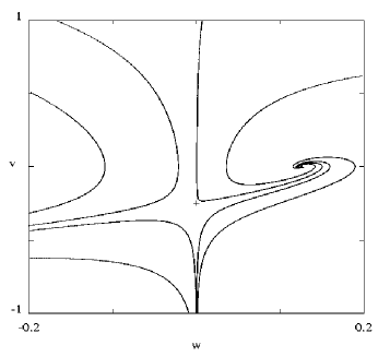
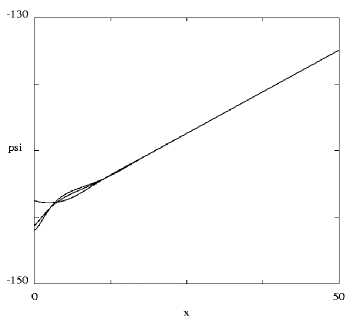
Figure 1: Numerical plots of the phase space in the $(w,v)$ coordinates, and the $\psi$ evolution with $x=log(t)$ for $n=\frac{1}{2}$ .The ’$+$’ sign is a saddle point and the triangle is a stable node.

But in the case of a universe containing the balance of matter and radiation, displayed by our own, it need not be the case that the asymptotic behaviour, displayed by the exact solution for the critical point, is reached before the radiation-dominated expansion is replaced by matter-domination, see references [10] and [9] for further discussion of this point. However as we discussed above these oscillations are an artefact of the linearisation process and the part of the solution (3.2.2) controlled by the constants $A$ and $B$ is only valid for small times, hence we called this behaviour pseudo-oscillatory.

3.2.3 Non-oscillatory behaviour

When $n\in(\frac{3}{5},\frac{2}{3})$, the $\psi$ field will approach its asymptotic behaviour in a non-oscillatory fashion as $t\rightarrow\infty$:

$$\psi(t) = \frac{1}{2}\ln[\frac{2N}{\left(1-3n\right)\left(3n-2\right)}]$$

$$+\frac{1}{2}\left(2-3n\right)\ln(t)+t^{\delta-\gamma}\left(A+B{t^{2\gamma}}\right)$$

where

$$\delta = {\frac{1-3n}{2}}$$ (32)

$$\gamma = \frac{1}{2}\sqrt{9-42n+45{n^{2}}}$$ (33)

Note that $\delta+\gamma<0$ in the domain $n\in(\frac{1}{3},\frac{2}{3})$, so at late times ($t\rightarrow\infty$), both the pseudo-oscillatory and non-oscillatory solutions case will approach the asymptotic solution defined by the appropriate value of $n$.

3.2.4 Intermediate behaviour

A transition between the pseudo-oscillatory and non-oscillatory regimes happens when $\beta=0$ and $n=\frac{3}{5}$; the $\psi$ field then has the following solution in the vicinity of the critical point:

$$\psi(t)=\frac{1}{5}\ln(N)+\frac{1}{10}\ln(t)+At^{-{\frac{2}{5}}}.$$ (34)

The phase plane structure and evolution of $\psi$ vs. $\ln t$ for this case are shown in Figure 2.

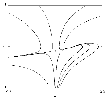
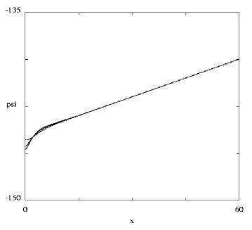
Figure 2: Numerical plots of the phase space in the $(w,v)$ coordinates, and the $\psi$ evolution with $x=log(t)$ for $n=\frac{3}{5}$. The ’$+$’ sign is a saddle point and the triangle is a stable node.

3.2.5 Overview

The late-time solution of the $\psi$ field solution is given by asymptotic behaviour of equations (3.2.2) or (3.2.3), which is:

$$\psi\rightarrow\frac{1}{2}\ln[\frac{2N}{\left(1-3n\right)\left(3n-2\right)}]+\frac{1}{2}\left(2-3n\right)\ln(t)$$

This shows that the solutions (3.2.2) and (3.2.3) generalise the ones found in [9], since they can be obtained setting $A=B=0$ in (3.2.2). In particular, the case of a radiation-dominated Universe ($n=\frac{1}{2}$), we have from (3.2.2):

$$\psi(t) = \frac{1}{2}\left(\log(8)+\log(N)+\log(t)\right)$$

$$+{t^{{-\frac{1}{4}}}}\left(B\cos[{\frac{5\sqrt{3}\log(t)}{4}}]+A\sin[{\frac{5\sqrt{3}\log(t)}{4}}]\right)$$

A full mathematical summary of the change in structure of the phase space with changing $n$ for the system (8) is given in the Appendix. There we include cosmologically unphysical values of $n$ and show how the critical point structure bifurcates with the change in value of $n$.

3.3 The Critical Points at Infinity

In order to describe the qualitative evolution of the system, we must determine the behaviour of the system (24) near the critical point $(u_{c},v_{c})=(+\infty,0)$. In order to bring the critical point to a finite value, we define:

$$u=-\frac{1}{2}\ln(w)$$

Using the new coordinate $w$ we can re-write the system (24) as:

$$\frac{dw}{dx} = -2wv$$ (36)

$$\frac{dv}{dx} = \left(1-3n\right)\left(1-{\frac{3n}{2}}+v\right)+w$$

This system has critical points on the $(w,v)$ plane when $(0,-1+{\frac{3n}{2}})$ and $(\left(1-3n\right)\left({\frac{3n}{2}}-1\right),0)$. Note that the second critical point is just the same as the one we have analysed in the previous section. In this subsection we will then only analyse the critical point $(w_{c},v_{c})=(0,-1+{\frac{3n}{2}})$ since it corresponds to the case where $u\rightarrow+\infty$.

Proceeding as before, and linearising (36) about $(w_{c},v_{c})=(0,-1+{\frac{3n}{2}})$ we obtain:

$$\frac{dW}{dx} = (2-3n)W$$ (37)

$$\frac{dV}{dx} = W+(1-3n)V$$

where $V=v-v_{c}$ and $W=w-w_{c}$. Again, the characteristic matrix of the system is non singular, and the critical point is simple. Hence, system (37) will have the same phase portrait as (36) in the neighbourhood of the critical point.

The eigenvalues $\xi_{1,2}$ and corresponding eigenvectors $\chi^{\xi_{1,2}}$ of the system (37) are:

$$\xi_{1} = 1-3n,\hskip 72.26999pt\chi^{\xi_{1}}=(0,1)$$ (38)

$$\qquad\xi_{2} = 2-3n,\hskip 72.26999pt\chi^{\xi_{2}}=(1,1)$$ (39)

These eigenvalues are always real. The critical point is an attractive node for $n>\frac{2}{3}$, a saddle point when $n\in(\frac{1}{3},\frac{2}{3})$, and it will be an unstable point when $n<\frac{1}{3}$. The general solution of the system (36) in the neighbourhood of the critical point $(w_{c},v_{c})=(0,-1+{\frac{3n}{2}})$, can be expressed as:

$$(w(x)-w_{c},v(x)-v_{c})=A{e^{\xi_{1}x}}\chi_{1}+B{e^{\xi_{2}x}}\chi_{2}$$

where $A$, $B$ are arbitrary constants and $x=\ln(t)$. Therefore, near the critical point $(u_{c},v_{c})=(+\infty,0)$:

$$\psi(t)=\frac{1}{2}\ln(\frac{N}{B})$$ (40)

so the scalar field is constant.

Note that in the domain $n\in(\frac{1}{3},\frac{2}{3})$ this is just a transitory solution since the critical point is a saddle point. In the domain $n<\frac{1}{3}$ it is an unstable critical point, possibly relevant as an early-time solution to braneworld cosmologies in the high-density regime where the Hubble expansion rate of the universe is linearly proportional to the density, so $n=1/4$ for a braneworld containing radiation, $n=1/12$ for a massless scalar field, and $n=1/6$ for dust. However, in the $t\rightarrow 0$ limit the assumption that the $\dot{\psi}^{2}$ and $\zeta\exp[-2\psi]$ terms can be neglected in the Friedmann equation (3) will break down.

3.3.1 The cases of $n>2/3$ and de Sitter expansion

An interesting case exists when $n>\frac{2}{3}$, since the critical point is a stable attractor and so this means that the constant-$\psi$ behaviour (40) is the late-time attractor, in agreement with the conclusions of references [10] and [9]. This is an important feature of a universe which exhibits accelerated expansion in its late stages ($n>1$). It means that the present value of $\alpha$ is the asymptotic one. It also means that variations in $\alpha$ are turned off by the domination of the expansion dynamics by negative curvature or by any quintessence field [10], [9]. This property may provide important clues to explaining why our universe possesses small but finite curvature or quintessence energy today: if it did not then the fine structure constant would continue to increase until it was impossible for atoms and molecules to exist [8].

In the $n>2/3$ case we can find a detailed asymptotic solution for equation (21) which has the form

$$\psi=C+B(t+t_{0})^{1-3n}+\frac{N\exp[-2C]}{2-3n}(t+t_{0})^{2-3n}$$

with $C,t_{0}$ constants. We see immediately that for this solution $\psi$ approaches a constant as $t\rightarrow\infty$. Of particular interest is the case of a curvature-dominated open universe, which has $n=1$. The phase plane structure and the evolution of $\psi$ vs. $\ln t$ for this case are shown in Figure 3.

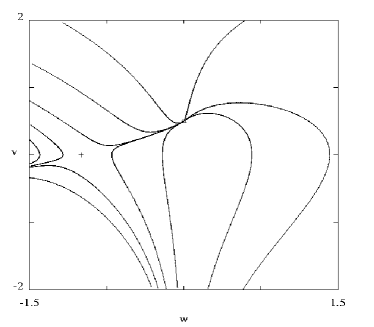
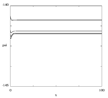
Figure 3: Numerical plots of the phase space in the $(w,v)$ coordinates, and the $\psi$ evolution with $x=log(t)$ for $n=1$. The ’$+$’ sign is a saddle point and the triangle is a stable node.

We see that this approach to constant behaviour occurs for all universes that accelerate ($n>1$) and so we would expect to find it also in the case of a de Sitter background universe with

$$a(t)=\exp[\lambda t]$$

where $\lambda>0$ is constant.

Substituting this in equation (8) we find a late-time asymptotic solution

$$\psi=C+B\exp[-3\lambda t]-\frac{N\left(3\lambda t+1\right)}{9\lambda^{2}}\exp[-2C-3\lambda t]\rightarrow C$$

as $t\rightarrow\infty.$

Notice that we were not able to fully describe the nature of this critical point in the cases where $n=\frac{1}{3}$ or $n=\frac{2}{3}$ since one of the eigenvalues of the systems is zero. In order to do so, we will study these two cases individually, in particular the case $n=\frac{2}{3}$ is important since it describes the scale factor evolution on a dust dominated universe.

3.3.2 The $n=\frac{1}{3}$, $a(t)=t^{\frac{1}{3}}$ case: an exact solution

The $n=\frac{1}{3}$ case can be exactly integrated. It is of interest as an exact solution in its own right but it corresponds to the case of a universe whose expansion dynamics are dominated by the effects of a fluid with a $p=\rho$ equation of state, or a massless scalar field. It also describes the behaviour of the $\psi$ field in an anisotropic universe of the simple Kasner type. We see when $n=1/3$ the system (24) has the form:

$$\frac{dv}{dx}=e^{-2u}$$ (41)

$$\frac{du}{dx}=v$$

This integrates to give

$$v^{2}+e^{-2u}=E^{2}$$

where $E$ is a constant. Hence, we have two possible solution branches: $v(u)=\pm\sqrt{E-e^{-2u}}$. Both, positive ($+$) and negative ($-$) solutions for $v$ lead to the same result. Choosing the positive branch of the $v(u)$ solution and using equations (41) we obtain:

$$u(x)=-\ln(E)+\ln[\cosh\left(E\left(C_{1}-x\right)\right)]$$

where $C_{1}$ is an integration constant. From (22) we have a solution for $\psi(t)$:

$$\psi(t)={\frac{\ln(\frac{N}{4})\ }{2}}-\ln(E)+\frac{1}{2}\ln(t)+\ln[\exp[EC_{1}]t^{-E}+t^{E}\exp[-EC_{1}]]$$

and the asymptotic limit when $t\rightarrow\infty$ gives

$$\psi(t)\rightarrow(\frac{1}{2}+E)\ln(t+t_{0}).$$

with $t_{0}$ constant. The phase space and $\psi(t)$ vs. $\ln t$ evolution is shown in Figure 4.

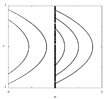
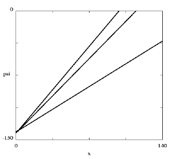
Figure 4: Numerical plots of the phase space in the $(w,v)$ coordinates and time evolution of $\psi(x)$ $n=\frac{1}{3}$. The central line which passes through the origin is an attractor for $w>0$, and an unstable line for $w<0$.

3.3.3 The $n=\frac{2}{3}$ , $a=t^{\frac{2}{3}}$ case

The case of a dust-dominated universe is mathematically special because of the presence of a zero eigenvalue in the stability analysis. It is illuminating to consider this case separately with an asymptotic analysis that extends the earlier study in [9]. Consider equation (21) with $n=2/3$. If we introduce the new variable $x=\ln(t),$ then

$$\psi^{\prime\prime}+\psi^{\prime}=N\exp[-2\psi]$$ (42)

At large $x$, the asymptotic form of this equation has the form:

$$\psi=\frac{1}{2}\ln[2N(x+x_{0})]-\frac{1}{2}\sum_{n=1}^{\infty}\frac{(n-1)!}{(x+x_{0})^{n}}+C\exp[-x]$$ (43)

where $C$ and $x_{0}>0$ are arbitrary constants. The leading order behaviour as $t\rightarrow\infty$ is therefore (cf.(11))

$$\psi\sim\frac{1}{2}\ln[2N\ln(t)]$$

Stability analysis of the $n=2/3$ asymptote

Performing the coordinate transformation $u=-\frac{1}{2}\ln(w)$ on the system (24) when $n=2/3$, we have:

$$\frac{dv}{dx} = w-v$$ (44)

$$\frac{dw}{dx} = -2vw$$

This system has a critical point at the origin of the $(w,v)$ plane. It corresponds to the case where $u\rightarrow\infty$. The linearisation about this critical point gives two eigenvalues: $\lambda_{1}=-1$ with the eigenvector $\chi_{1}=(0,1)$ and $\lambda_{2}=0$ with the eigenvector $\chi_{2}=(1,1)$ . Since we have a zero eigenvalue, the stability is determined by the non-linear behaviour and is one of Lyapunov’s ’critical’ cases [27],[28] [29]. We apply a linear transformation to split the system into critical and non-critical variables; where the critical variables are those eigenvectors with zero eigenvalue and the non-critical variable are the others. Then we apply a non-linear transformation which will eliminate the influence of the critical variables upon the non-critical ones at the leading order. This gives $(w,v)\rightarrow(W,W+V)$, and the system (44) becomes:

$$W^{\prime} = -2W(W+V)$$ (45)

$$V^{\prime} = -V+2W(W+V)$$

with the critical point at $(W,V)=(0,0).$The Lyapunov procedure for the system (45) is to set the linearly stable variable, $V,$ equal to zero in the $W^{\prime}$ equation so,

$$W^{\prime}=-2W^{2}$$

and so the second-order analysis shows that critical point $(W,V)=(0,0)$ is unstable. In fact this critical point is a saddle point as can be seen from the numerical-phase-plane plot figure  5. The unstable part correspond to a non-physical range of the cosmological variables, since it gives $w<0$. The stable part corresponds to the range of values where $w\geq 0$. With respect to our (approximate) exact solution, the unphysical case will correspond to the range of $x_{0}<0$, since they lead to $\alpha<0$. Hence the asymptotic solution (43) is the stable late-time behaviour of the dust universes with small $\zeta.$ The phase plane structure and the evolution of $\psi$ vs. $\ln t$ is shown in Figure 5.

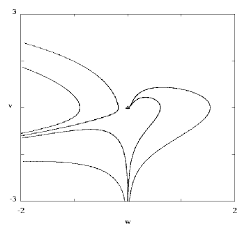
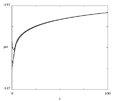
Figure 5: Numerical plots of the phase space in the $(w,v)$ coordinates, and the $\psi$ evolution with $x=log(t)$ for $n=\frac{2}{3}$. The triangle is a saddle point for $w<0$ and a stable node for $w>0$.

4 Some general asymptotic features

4.1 Models with asymptotically constant $\psi$ and $\alpha$

We have seen that $\psi$, and hence the fine structure constant, $\alpha$, tends to a constant at late times in accelerating universes with power-law and exponential increase of the scale factor. We can establish a useful general criterion for this asymptotic behaviour to occur for general $a(t)$. Suppose that as $t\rightarrow\infty$ both sides of equation (8) tend to a constant (which may be equal to zero). Thus

$$(\dot{\psi}a^{3})^{\cdot} = A$$

$$\psi = A\int\frac{tdt}{a^{3}}+B\int\frac{dt}{a^{3}}+C\rightarrow C$$

as $t\rightarrow\infty$ if

$$A\int\frac{tdt}{a^{3}} \rightarrow 0$$ (46)

$$B\int\frac{dt}{a^{3}} \rightarrow 0$$ (47)

Then for consistency we also require, as $t\rightarrow\infty$, that

$$N\exp[-2C]\rightarrow A$$

so $A$ cannot be chosen to be zero. Thus in all cosmological models for which (46) and (47) hold there will be a self-consistent asymptotic solution as $t\rightarrow\infty$ of the form

$$\psi=N\exp[-2C]\int\frac{tdt}{a^{3}}+B\int\frac{dt}{a^{3}}+C$$

where $B,C$ are positive constants. We see that the $n>2/3$ and de Sitter cases satisfy the conditions (46) and (47) hence $\psi$ is asymptotically constant. The dust ($n=2/3$) case, for which $\psi\rightarrow\infty$ as $t\rightarrow\infty$ satisfies (47) but violates (46).

5 Conclusions

Using a phase plane analysis we have studied the cosmological evolution of a time-varying fine-structure ’constant’ $\alpha(t)=\exp[2\psi]$, in the BSBM theory. We have considered the cases created by power-law evolution of the expansion scale factor of the universe. We have shown that in general $\alpha$ increases with time or asymptotes to a constant value at late times. We have found a new exact solution for the case of a universe dominated by a stiff fluid or massless scalar field. We have also found general asymptotic solutions for all the different and possible behaviours via the analysis of the critical points of the system that determines the evolution of $\alpha$. In particular, we have found asymptotic solutions for the dust, radiation and curvature-dominated FRW universe which also generalise the asymptotes found in [9].These solutions correspond to late-time attractors that describes the $\psi$ and $\alpha$ evolution in time and will enable a more detailed analysis to be made of the fit between theoretical expectations of varying $\alpha$ theories and observations of relativistic fine structure in atoms at high redshift.

Acknowledgements We would like to thank Håvard Sandvik and João Magueijo for discussions. DFM is supported by Fundação para a Ciência e a Tecnologia, Portugal, through the research grant BD/15981/98.

Appendix:  General analysis of the phase plane bifurcations

In previous sections we have analysed the $\psi$ evolution equation (8) for a range of variables which are physically realistic and correspond to expanding universes. We will now analyse the whole range for variables of the system (37). As before we see there are two critical points in the $(w,v)$ plane, at $(0,-1+{\frac{3n}{2}})$ and $((1-3n)(\frac{3n}{2}-1),0)$. Linearising (37) about $(w_{c_{1}},v_{c_{1}})=(0,-1+\frac{3n}{2})$ and $(w_{c_{2}},v_{c_{2}})=((1-3n)(\frac{3n}{2}-1),0)$ we obtain the following characteristics matrices:

$M_{1}=\bordermatrix{&&\cr&2-3n&0\cr&1&1-3n\cr}$   $M_{2}=\bordermatrix{&&\cr&0&(3n-1)(2-3n)\cr&1&1-3n\cr}$

The characteristic matrices are non singular except when $n=\frac{1}{3}$ or $n=\frac{2}{3}$. In the non-singular cases the critical points will be simple and the system defined by these differential equations is structurally stable [31], and there will be no ’strange’ chaotic behaviour outside the neighbourhood of the critical points. Hence, the linearised system will have the same phase portrait as non-linearised one in the neighbourhood of the critical points.

The evolution, with respect to changing $n$, of the signs of the determinant and the trace of these two matrices is given in the table. This show us that there are always two critical points in our system, an unstable saddle and an attractor (which changes from a spiral to a node).

$n$	Critical Points $(w_{c},v_{c})$
	$\left(\left(3n-1\right)\left(1-\frac{3n}{2}\right),0\right)$	$\left(0,1-\frac{3n}{2}\right)$
$(-\infty;\frac{1}{3})$	Saddle Point (non-physical)	Unstable Node
	det $M_{1}<0$, Tr $M_{1}>0$	det $M_{2}>0$, Tr $M_{2}>0$
$\frac{1}{3}$	Origin	Axis
	det $M_{1}=0$, Tr $M_{1}=0$	det $M_{2}=0$, Tr $M_{2}>0$
$(\frac{1}{3};\frac{1}{2})$	Stable Spiral	Saddle Point
	det $M_{1}>0$, Tr $M_{1}<0$	det $M_{2}<0$, Tr $M_{2}>0$
$\frac{1}{2}$	Stable Spiral	Saddle Point
	det $M_{1}>0$, Tr $M_{1}<0$	det $M_{2}<0$, Tr $M_{2}=0$
$(\frac{1}{2};\frac{3}{5})$	Stable Spiral	Saddle Point
	det $M_{1}>0$, Tr $M_{1}<0$	det $M_{2}<0$, Tr $M_{2}<0$
$\frac{3}{5}$	Stable Spiral (node)	Saddle Point
	det $M_{1}>0$, Tr $M_{1}<0$	det $M_{2}<0$, Tr $M_{2}<0$
$(\frac{3}{5};\frac{2}{3})$	Stable Node	Saddle Point
	det $M_{1}>0$, Tr $M_{1}<0$	det $M_{2}<0$, Tr $M_{2}<0$
$\frac{2}{3}$	Stable Axis	Stable Axis
	det $M_{1}=0$, Tr $M_{1}<0$	det $M_{2}=0$, Tr $M_{2}<0$
$(\frac{2}{3};\infty)$	Saddle Point (non-physical)	Stable Node
	det $M_{1}<0$, Tr $M_{1}<0$	det $M_{2}>0$, Tr $M_{2}<0$

The cases $n=\frac{1}{3}$ or $n=\frac{2}{3}$, where the determinant of the characteristic matrixes vanishes, lead to a bifurcation of codimension $1$, in particular, of Saddle-Node type [30], since they correspond to points where the determinants of the characteristic matrices change sign, det$M_{1}$ $=$ det$M_{2}=0$. At these values of $n$ the nature of the system will change. Cosmologically, these points represent a change in the behaviour of the time evolution of the fine structure ’constant’ as can be seen from the figures: 6, 4, 1, 2, 5, 3, which display the time evolution of $\psi$. When $n$ starts to grows from $-\infty$ to $\frac{1}{3}$ the two critical points slowly converge at $n=\frac{1}{3}$. For example, in the $n=0$ case where we may without loss of generality set $a=1$, equation (8) has the exact solution

$$\alpha=\exp[2\psi]=A^{-2}\cosh^{2}[AN^{1/2}(t+t_{0})]$$

where $A,t_{0}$ are constants. This is an unrealistically rapid growth asymptotically , $\psi\varpropto t,$caused by the absence of the inhibiting effect of the cosmological expansion. The case of $n=1/4$ is shown in Figure 6, which shows the phase space trajectories and the evolution of $\psi$ vs. $\ln t.$

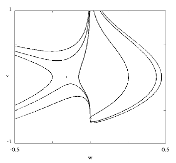
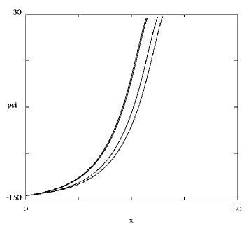
Figure 6: Numerical plots of the phase space in the $(w,v)$ coordinates, and the $\psi$ evolution with $x=log(t)$ for $n=\frac{1}{4}$. The ’$+$’ sign is a saddle point and the square is an unstable source.

At $n=\frac{1}{3}$ we are in the situation where the two critical points collapse into a unique one at the origin, creating a saddle-node bifurcation and a concomitant change in the behaviour and evolution of $\psi$. As $n$ keeps growing the single critical point splits into two critical points again. They move apart until the radiation value is reached, $n=\frac{1}{2}$ (Tr $M_{2}=0$). In this case, $\psi$ is a asymptotically monotonic growing function of time, with some small oscillations near the Planck epoch. However, note that in our universe the asymptote giving an increase of $\psi$ behaviour with time is never reached before the dust-dominated evolution takes over [10], [9], [8].

As the universe evolves to the dust-dominated epoch, and $n$ approaches the intermediate behaviour $n=\frac{3}{5}$, the two critical points start to coalesce again into a single point. When $n=\frac{3}{5}$ is reached, $\psi$ becomes a strictly monotonically growing function of time. When $n$ reaches the value corresponding to a dust-dominated universe, $n=\frac{2}{3}$, another saddle-node bifurcation occurs. The two critical points collapse into a single one. Again there will be change in the behaviour of $\psi$ for larger values of $n$. Accordingly, when $n>2/3,$ the two critical points reappear once again and $\psi$ becomes asymptotically constant in value.

Notice, that although a bifurcation is something that ’spoils’ the smooth behaviour of a system, in our case, that won’t happen, due to the physical constraints of our variables. In reality due to those constraints, the physical system will never ’feel’ the abrupt change at $n=\frac{1}{3}$ and $n=\frac{2}{3}$. This is also due to the fact that the attracting critical point always lies in the physical range of the variables, while the unstable one disappears form the physical system when the bifurcations occur, as can be seen from the phase plane plots.

References

- [1] M. Murphy, J. Webb, V. Flambaum, V. Dzuba, C. Churchill, J. Prochaska, A. Wolfe, MNRAS, 327, 1208 (2001)
- [2] J.K. Webb, M.T. Murphy, V.V. Flambaum, V.A. Dzuba, J.D. Barrow, C.W. Churchill, J.X. Prochaska, A.M. Wolfe, Phys. Rev. Lett. 87, 091301 (2001).
- [3] J.K. Webb, V.V. Flambaum, C.W. Churchill, M.J. Drinkwater J.D. Barrow, Phys. Rev. Lett. 82, 884 (1999).
- [4] J. Moffat, Int. J. Mod. Phys. D 2, 351 (1993).
- [5] A. Albrecht and J. Magueijo, Phys. Rev. D 59, 043516 (1999).
- [6] J.D. Barrow, Phys. Rev. D 59, 043515 (1999).
- [7] J. D. Barrow, J. Magueijo and H. B. Sandvik, Variations of Alpha in Space and Time, astro-ph/0202129.
- [8] J. D. Barrow, H. B. Sandvik and J. Magueijo, Phys. Rev. D 65, 123501 (2002) .
- [9] J. D. Barrow, H. B. Sandvik and J. Magueijo, Phys. Rev. D 65, 063504 (2002) .
- [10] H. B. Sandvik, J. D. Barrow and J. Magueijo, Phys. Rev. Lett. 88, 031302 (2002).
- [11] J. Magueijo, J. D. Barrow and H. B. Sandvik, Is it e or is it c? Experimental Tests of Varying Alpha, astro-ph/0202374.
- [12] G. Dvali and M. Zaldarriaga, Phys. Rev. Lett. 88 091303 (2002).
- [13] J. Moffat, A Model of Varying Fine Structure Constant and Varying Speed of Light, astro-ph/0109350.
- [14] T. Banks, M. Dine, M.R. Douglas, Phys. Rev. Lett. 88, 131301 (2002).
- [15] P. Langacker, G. Segre and M. Strassler, Phys. Lett. B 528, 121-128 (2002); X. Calmet and H. Fritzsch, The Cosmological Evolution of the Nucleon Mass and the Electroweak Coupling Constants, hep-ph/0112110.
- [16] K. Olive and M. Pospelov, Phys. Rev. D 65 085044 (2002).
- [17] J.D. Bekenstein, Phys. Rev. D 25, 1527 (1982).
- [18] J.D. Barrow and J. Magueijo. Phys. Lett. B 447, 246 (1999).
- [19] J.D. Barrow and J. Magueijo, Phys. Lett. B 443, 104 (1998).
- [20] J. Magueijo, Phys. Rev. D 62, 103521, (2000).
- [21] J. Magueijo, Phys. Rev. D 63, 043502, 2001.
- [22] J.Magueijo, H. Sandvik, and T. Kibble, Phys. Rev. D 64, 023521, 2001.
- [23] C. Will, Theory and experiment in gravitational physics, CUP, Cambridge (1993).
- [24] S. Alexander and J. Magueijo, Non-commutative geometry as a realization of varying speed of light cosmology, hep-th/0104093.
- [25] P.P. Avelino et. al., Phys. Rev. D 62, 123508, (2000) and Phys. Rev. D 64 103505 (2001).
- [26] R. Battye, R. Crittenden, J. Weller, Phys. Rev. D 63, 043505.
- [27] J. D. Barrow and D. H. Sonoda, Phys. Repts., 139,1, (1986).
- [28] I. Bendixson, Acta Math. 24, 1 (1901)
- [29] E. A. Jackson, Perspectives of Nonlinear Dynamics, vol. 1, CUP, Cambridge, (1992).
- [30] S. Wiggins, Introduction to applied nonlinear dynamical systems and chaos, Springer-Verlag, NY (1990).
- [31] A. A. Andronov, E. A. Leontovich, L. L. Gordon and A. G. Maier, Qualitative Theory of Second-Order Dynamic Systems, Wiley NY, (1973).