Binary black hole initial data for numerical general relativity based on post-Newtonian data

Abstract

With the goal of taking a step toward the construction of astrophysically realistic initial data for numerical simulations of black holes, we for the first time derive a family of fully general relativistic initial data based on post-2-Newtonian expansions of the 3-metric and extrinsic curvature without spin. It is expected that such initial data provide a direct connection with the early inspiral phase of the binary system. We discuss a straightforward numerical implementation, which is based on a generalized puncture method. Furthermore, we suggest a method to address some of the inherent ambiguity in mapping post-Newtonian data onto a solution of the general relativistic constraints.

I Introduction

One of the most exciting scientific objectives of gravitational wave astronomy involves the search for and detailed study of signals from sources that contain binary black holes. Mergers of two black holes both with masses of $\sim 10-100M_{\odot}$ will be observable by the ground based gravitational wave detectors, such as GEO600, LIGO and others Schutz (1999). These systems are highly relativistic once they enter the sensitive frequency band ($\sim 50-200\,{\rm Hz}$) of the detector. For LISA, gravitational waves from super-massive binary black hole mergers (e.g. black holes with mass greater than $10^{6}M_{\odot}$) are very strong, with high signal-to-noise ratios up to $10^{4}$ Hughes et al. (2001), making these events observable from almost anywhere in the universe. Astrophysically realistic models of binary black hole coalescence are therefore required to study these phenomena in detail Éanna É. Flanagan and Hughes (1998).

To solve the full Einstein equations in the dynamic, non-linear phase at the end of the binary black hole inspiral we turn to numerical relativity. Numerical relativity has advanced to the point where a time interval of up to $40M$ (where $M$ is the total mass) of the merger phase of two black holes can be computed if the black holes start out close to each other Brügmann (1999); Brandt et al. (2000); Alcubierre et al. (2001). Recent simulations of head-on collisions of black holes last significantly longer and give reason for optimism for the orbiting case Alcubierre et al. (2002). An approach to produce at least moderately accurate models for the wave forms generated in binary black hole mergers was recently developed in the so-called Lazarus project Baker and Campanelli (2000); Baker et al. (2000, 2002b, 2001, 2002a), a technique that bridges ‘close’ and ‘far’ limit approximations with full numerical relativity. This approach has lead to the first approximate theoretical estimates for the gravitational radiation wave forms and energy to be expected from the plunge of orbiting non-spinning binary black holes to coalescence Baker et al. (2001, 2002a).

Due to theoretical and numerical limitations, all current numerical simulations must begin by specifying initial data when the black holes are already very close (separation $\lesssim 7M$). There is a push to place the starting point of these simulations at earlier times, say at a few orbits before a fiducial innermost stable circular orbit (ISCO) which approximately marks the transition from the inspiral phase to the plunge and merger. But whatever the starting point, the simulation will only be astrophysically meaningful if it starts with astrophysically realistic initial data.

The question we want to address in this paper is therefore how to obtain astrophysically realistic initial data for numerical simulations of binary black hole systems. In general relativity the initial data must fulfill constraint equations, so only part of the data are freely specifiable, and the rest is determined by solving the constraint equations (for a review see e.g. Cook (2000)). A lot of the work in constructing initial data has focused on approaches that pick the freely specifiable part of the data with the aim of simplifying the constraint equations, rather than using astrophysically realistic initial data. A standard assumption is that the 3-metric is conformally flat and the extrinsic curvature is derived from a purely longitudinal ansatz (see e.g. Cook (2000); Bowen and York (1980); Cook (1994); Brandt and Brügmann (1997)). Currently, there are a number of new approaches  Marronetti and Matzner (2000); Grandclement et al. (2001); Cook (2001); Dain (2001); Dain et al. (2002) to specify ‘improved’, including non-conformally flat, initial data for binary black holes.

However, none of these approaches to construct initial data makes explicit use of information from an approximation procedure such as the post-Newtonian (PN) method, which is believed to accurately represent astrophysical systems in the limit of slow-moving/far-apart black holes. An approximate binary black hole metric based on post-1-Newtonian (1PN) information in a corotating gauge has been derived by Alvi Alvi (2000). However, at present this metric cannot be used in numerical simulations due to the presence of discontinuities in the matching regions Jansen . An interesting approach based on quasi-equilibrium sequences of initial data has been studied numerically, e.g. Duez et al. (2001), although some aspects of the method appear to be based on Newtonian or 1PN assumptions.

In this paper we describe a method to generate new fully general relativistic initial data for two inspiraling black holes from PN expressions. The motivation for this method is that even though PN theory may not be able to evolve two black holes when they get close, it can still provide initial data for fully nonlinear numerical simulations when we start at a separation where PN theory is valid. In particular, we obtain an explicit far limit interface for the Lazarus approach. Our method allows us to incorporate information from the PN treatment and should eventually provide a direct connection to the inspiral radiation.

Like in other approaches, we start from expressions for the 3-metric and extrinsic curvature in a convenient gauge. We use expressions for the 3-metric and its conjugate momentum up to PN order $(v/c)^{5}$, computed in the canonical formalism of ADM by Jaranowski and Schäfer Jaranowski and Schäfer (1998). This order corresponds to 2.5PN in the 3-metric and 2PN in the conjugate momentum, since the latter contains a time derivative. Therefore, the PN data are accurate to 2PN.

The 3-metric and its conjugate momentum are derived together with a two-body Hamiltonian using coordinate conditions Ohta et al. (1974); Schäfer (1985); Damour et al. (2001a), which correspond to the ADM transverse-traceless (ADMTT) gauge. Note that there are several other formulations and gauges for PN theory, see e.g. Blanchet (2002) for a review. The ADMTT gauge has several advantages: (i) we can easily find expressions for 3-metric and extrinsic curvature, (ii) unlike in the harmonic gauge no logarithmic divergences appear, (iii) for a single black hole the data simply reduce to Schwarzschild in standard isotropic coordinates, (iv) up to $(v/c)^{3}$ the data look like in the puncture approach Brandt and Brügmann (1997), which simplifies calculations, and (v) the trace of the extrinsic curvature vanishes up to order $(v/c)^{6}$, so that we can set it to zero (if we go only up to order $(v/c)^{5}$), which can be used to decouple the Hamiltonian constraint equation from the momentum constraint equations. In the ADMTT gauge the 3-metric is conformally flat up to order $(v/c)^{3}$, at order $(v/c)^{4}$ deviations from conformal flatness enter. The extrinsic curvature up to order $(v/c)^{3}$ is simply of Bowen-York form Bowen and York (1980), with correction terms of order $(v/c)^{5}$.

We will use the York-Lichnerowicz conformal decomposition York (1973) and use the PN data as the freely specifiable data. We numerically solve for a new conformal factor $\Psi$ and the usual correction to the extrinsic curvature, given by a vector potential $W^{i}$. The new extrinsic curvature and the 3-metric multiplied by $\Psi^{4}$ are then guaranteed to fulfill the constraints. The real problem in this approach is to find a numerical scheme which can deal with the divergences in the PN data at the center of each black hole. The most serious divergence occurs in the PN conformal factor $\psi_{PN}$ of the conformally flat part of the 3-metric. We therefore rescale the PN data by appropriate powers of $\psi_{PN}$ to generate a well behaved 3-metric. If we then use the conformally rescaled data as the freely specifiable data and make the ansatz that the new conformal factor $\Psi$ is the PN conformal factor $\psi_{PN}$ plus a finite correction $u$, we arrive at elliptical equations which can be solved numerically. The splitting of the new conformal factor into $\Psi=\psi_{PN}+u$ is very similar to the puncture approach Brandt and Brügmann (1997), except that in our case the momentum constraint has to be solved numerically as well.

Let us point out several issues that arise in the construction of solutions to the constraints of the full theory based on PN data. First of all, the accuracy of the PN approximation increases with the separation of the binary, and the same is therefore true for the numerical data. Second, PN theory typically deals with point particles rather than black holes. One has to somehow introduce black holes into the theory, which leads to a certain arbitrariness of the data near the black holes. We make the specific choice contained in Jaranowski and Schäfer (1998). Note that since we are solving elliptic equations, the data near the black holes affect the solution everywhere. Third, some of the PN expressions that we use are near zone expansions which are invalid far from the particles. This means we have data only in a limited region of space.

Finally, the reader should be aware of the following basic feature of the York procedure to compute initial data. Given valid free data, which in our case is derived from the PN data, the procedure projects the data onto the solution space of the constraints. This projection maps the PN data somewhere, but is the end point better than the starting point? We have to make sure that we do not loose the advantage of starting with PN data over, say, simply using PN orbital parameters in the conformally flat data approach. After describing and resolving several technical issues in the construction of our data set, we will therefore (i) quantify the ‘kick’ from PN to fully relativistic data, and (ii) suggest a concrete method for improving the results of our straightforward first implementation.

I.1 Notation

We use units where $G=c=1$. Lowercase Latin indices denote the spatial components of tensors. The coordinate locations of the two particles are denoted by $(x_{1},y_{1},z_{1})$ and $(x_{2},y_{2},z_{2})$. We define

$$r_{A}:=\sqrt{(x-x_{A})^{2}+(y-y_{A})^{2}+(z-z_{A})^{2}}.$$ (1)

and

$$n_{A}^{i}:=(x-x_{A},y-y_{A},z-z_{A})/r_{A},$$ (2)

where the subscript $A$ labels the particles. Furthermore we introduce

$$r_{12}:=\sqrt{(x_{1}-x_{2})^{2}+(y_{1}-y_{2})^{2}+(z_{1}-z_{2})^{2}}$$ (3)

to denote the separation between the particles. All terms carrying a superscript $TT$ are transverse traceless with respect to the flat 3-metric $\delta_{ij}$.

II The PN expressions for 3-metric and extrinsic curvature

Our starting point is the expressions for the PN 3-metric $g^{PN}_{ij}$ and the PN 3-momentum $\pi_{PN}^{ij}$ computed in the ADMTT gauge Jaranowski and Schäfer (1998). The ADMTT gauge is specified by demanding that the 3-metric has the form

$$g^{PN}_{ij}=\psi_{PN}^{4}\delta_{ij}+h_{ij}^{TT}.$$ (4)

and that the conjugate momentum fulfills

$$\pi_{PN}^{ij}\delta_{ij}=0.$$ (5)

We explicitly include the formal PN expansion parameter $\epsilon\sim v/c$ in all PN expressions, a subscript in round brackets will denote the order of each term. When a PN term is evaluated numerically, $\epsilon$ is set to one.

We start with the PN expression for the 3-metric Jaranowski and Schäfer (1998)

$$g^{PN}_{ij}=\psi_{PN}^{4}\delta_{ij}+\epsilon^{4}h_{ij(4)}^{TT}+\epsilon^{5}h_{ij(5)}^{TT}+O(\epsilon^{6}),$$ (6)

where the conformal factor of PN theory is given by

$$\psi_{PN}=1+\frac{1}{8}\left(\epsilon^{2}\phi_{(2)}+\epsilon^{4}\phi_{(4)}\right)+O(\epsilon^{6}).$$ (7)

Using the expressions for $\phi_{(2)}$ and $\phi_{(4)}$ given in Jaranowski and Schäfer (1998) we see that the conformal factor $\psi_{PN}$ can be written in the simple form

$$\psi_{PN}=1+\sum_{A=1}^{2}\frac{E_{A}}{2r_{A}}+O(\epsilon^{6}),$$ (8)

where the constants $E_{1}$ and $E_{2}$ depend only on the masses $m_{1}$, $m_{2}$, the momenta $p_{1}$, $p_{2}$ and the separation $r_{12}$ of PN theory. They are given by

$$E_{A}=\epsilon^{2}m_{A}+\epsilon^{4}\left(\frac{p_{A}^{2}}{2m_{A}}-\frac{m_{1}m_{2}}{2r_{12}}\right)$$ (9)

and can be regarded as the energy of each particle.

Note that the PN 3-metric is singular at the location of each particle, since $\phi_{(2)}$, $\phi_{(4)}$ and $h_{ij(4)}^{TT}$ all go like $\sim 1/r_{A}$ as particle $A$ is approached, and $h_{ij(5)}^{TT}$ is regular. This means that the strongest singularity is in $\psi_{PN}^{4}\sim 1/r_{A}^{4}$ and that the $\psi_{PN}^{4}$ term dominates near each particle. Hence near each particle the 3-metric can be approximated by

$$g^{PN}_{ij}\approx\left(1+\frac{E_{A}}{2r_{A}}\right)^{4}\delta_{ij}+O(1/r_{A}^{3}),$$ (10)

which is just the Schwarzschild 3-metric in isotropic coordinates. For $r_{A}\rightarrow 0$ we approach the coordinate singularity that represents the inner asymptotically flat end of Schwarzschild in isotropic coordinates, which is also called the puncture representation of Schwarzschild. This shows that if we write the 3-metric as in Eq. (6), we actually do have a black hole centered on each particle. This is non-trivial since PN theory in principle only describes particles.

On the other hand, if we expand the conformal factor in Eq. (6), the puncture singularity of Schwarzschild is no longer present. If we insert Eq. (7) into Eq. (6) and expand in $\epsilon$ we obtain

$$g^{PN}_{ij} = \left[1+\epsilon^{2}\frac{1}{2}\phi_{(2)}+\epsilon^{4}\left(\frac{1}{2}\phi_{(4)}+\frac{3}{32}\phi_{(2)}^{2}\right)\right]\delta_{ij}$$ (11)

$$+\epsilon^{4}h_{ij(4)}^{TT}+\epsilon^{5}h_{ij(5)}^{TT}+O(\epsilon^{6}),$$

which goes like

$$g^{PN}_{ij}\approx\left(\frac{\mbox{const}}{r_{A}^{2}}\right)\delta_{ij}+O(1/r_{A}),$$ (12)

near each particle. One necessary condition for a black hole is the presence of a marginally trapped surface, and while the Schwarzschild metric in isotropic coordinates has a minimal surface at radius $M/2$, the term in $1/r_{A}^{2}$ in (12) leads to a minimum in area at radius zero (ignoring the extrinsic curvature terms). Therefore the particle is not necessarily surrounded by a horizon.

From now on we will use the 3-metric of Jaranowski and Schäfer (1998) as written in Eq. (6), without expanding $\psi_{PN}^{4}$ in $\epsilon$, in order to make sure that we have black holes in our data. The puncture coordinate singularity has replaced the point particle singularity. This choice is somewhat ad hoc, but since PN theory is not valid near the particles anyway, we have to make some choice, and putting in black holes as punctures seems natural.

The determinant of $g^{PN}_{ij}$ is

$$g^{PN}=\psi_{PN}^{12}+O(\epsilon^{6}),$$ (13)

since $\delta^{ij}h_{ij}^{TT}=0$.

The PN expansion for the conjugate momentum is Jaranowski and Schäfer (1998)

$$\pi_{PN}^{ij}=\epsilon^{3}\tilde{\pi}^{ij}_{(3)}+\epsilon^{5}\tilde{\pi}^{ij}_{(5)}+\epsilon^{5}\pi^{ijTT}_{(5)}+O(\epsilon^{6}),$$ (14)

where

$$\tilde{\pi}^{ij}_{(5)}=-\frac{1}{2}\phi_{(2)}\tilde{\pi}^{ij}_{(3)}+\frac{1}{2}(\phi_{(2)}\tilde{\pi}^{ij}_{(3)})^{TT}$$ (15)

and

$$\pi^{ijTT}_{(5)}=\frac{1}{2}\dot{h}_{ij(4)}^{TT}+\frac{1}{2}(\phi_{(2)}\tilde{\pi}^{ij}_{(3)})^{TT}.$$ (16)

As in the case of the 3-metric it turns out that $\pi_{PN}^{ij}$ in Eq. (14) is singular, since $\tilde{\pi}^{ij}_{(3)}$, $\tilde{\pi}^{ij}_{(5)}$ and $\pi^{ijTT}_{(5)}$ all diverge at the location of each particle. But all these singularities in $\pi_{PN}^{ij}$ up to $O(\epsilon^{5})$ can be removed by rewriting Eq. (14) as Schäfer

$$\pi_{PN}^{ij} = \psi_{PN}^{-4}\left[\epsilon^{3}\tilde{\pi}^{ij}_{(3)}+\epsilon^{5}\frac{1}{2}\dot{h}_{ij(4)}^{TT}+\epsilon^{5}(\phi_{(2)}\tilde{\pi}^{ij}_{(3)})^{TT}\right]$$ (17)

$$+O(\epsilon^{6}).$$

which can be verified to agree with Eq. (14) by re-expanding $\psi_{PN}$ as in Eq. (7) and keeping only terms up to $O(\epsilon^{5})$. Hence all singularities can be absorbed by the conformal factor, which is the basis for the puncture method in general Brandt and Brügmann (1997); Alcubierre et al. (2002).

Note that explicit expressions for $\phi_{(2)}$, $\phi_{(4)}$ and $\tilde{\pi}^{ij}_{(3)}$ can be found in e.g. Jaranowski and Schäfer (1998) or Ohta et al. (1974). In addition Ohta et al Ohta et al. (1974) also give an expression for the lapse up to $O(\epsilon^{4})$ and for the shift up to $O(\epsilon^{5})$. The explicit expressions for $h_{ij(4)}^{TT}$, $\dot{h}_{ij(4)}^{TT}$, and $\pi^{ijTT}_{(5)}$, however, we obtained from Jaranowski and Schäfer in a Mathematica file.

It should also be noted that the analytic expressions Jaranowski and Schäfer (1998) used for the PN terms $\phi_{(2)}$, $\phi_{(4)}$ and $\tilde{\pi}^{ij}_{(3)}$ are valid everywhere, while the expressions used for $h_{ij(4)}^{TT}$, $\dot{h}_{ij(4)}^{TT}$ and $h_{ij(5)}^{TT}$ are near zone expansions.

The near zone expansion is valid only for $r\ll\lambda\sim\pi\sqrt{r^{3}/(m_{1}+m_{2})}$, where $r$ is the distance from the particle sources and $\lambda$ is the wavelength. In principle $h_{ij}^{TT}$ should be computed from a wave equation, but in the near zone this equation can be simplified by replacing the d’Alembertian by a Laplacian. This is exactly what Jaranowski and Schäfer Jaranowski and Schäfer (1998) do to arrive at the expression for $h_{ij}^{TT}$ we use. In particular, the near zone expansion for $h_{ij(5)}^{TT}$ is a spatially constant tensor field that just varies in time. So for the purpose of finding initial data it suffices to choose the initial time such that $h_{ij(5)}^{TT}$ vanishes. Thus in all our numerical computations we will set $h_{ij(5)}^{TT}=0$.

Using the gauge condition (5) we obtain

$$\pi_{PN}=g^{PN}_{ij}\pi_{PN}^{ij}=O(\epsilon^{7}).$$ (18)

The next task is to compute the extrinsic curvature

$$K_{PN}^{ij}=-\frac{1}{\sqrt{g}}\left(\pi_{PN}^{ij}-\frac{1}{2}\pi_{PN}g^{ij}\right)$$ (19)

from the conjugate momentum $\pi_{PN}^{ij}$. With the help of Eqs. (13) and (18), and using the expressions for $\pi_{PN}^{ij}$ in Eq. (17) we find that the extrinsic curvature can be written as

$$K_{PN}^{ij} = -\psi_{PN}^{-10}\left[\epsilon^{3}\tilde{\pi}^{ij}_{(3)}+\epsilon^{5}\frac{1}{2}\dot{h}_{ij(4)}^{TT}+\epsilon^{5}(\phi_{(2)}\tilde{\pi}^{ij}_{(3)})^{TT}\right]$$ (20)

$$+O(\epsilon^{6}),$$

such that the conformal factor $\psi_{PN}$ is factored out. The leading term in Eq. (20) is of Bowen-York form, i.e.

$$-\tilde{\pi}^{ij}_{(3)} = \sum_{A=1}^{2}\frac{3}{2r_{A}^{2}}\left[p_{A}^{i}n_{A}^{j}+p_{A}^{j}n_{A}^{i}\right.$$ (21)

$$\quad\left.-p_{A}^{m}n_{A}^{n}\delta_{mn}(\delta^{ij}-n_{A}^{i}n_{A}^{j})\right].$$

Using that $\partial_{i}\tilde{\pi}^{ij}_{(3)}=0$ outside the singularities and the fact that the last two terms inside the square bracket of Eq. (20) are transverse (with respect to $\delta_{ij}$), we find

$$\partial_{i}(\psi_{PN}^{10}K_{PN}^{ij})=O(\epsilon^{6})$$ (22)

outside the singularities. Moreover from Eq. (18) we have

$$K_{PN}=g^{PN}_{ij}K_{PN}^{ij}=O(\epsilon^{7})$$ (23)

so that $K_{PN}^{ij}$ can be considered traceless up to $O(\epsilon^{6})$.

III Circular orbits in PN theory

The PN expressions given in section II are valid for general orbits. Any particular orbit is specified by giving the positions and momenta of the two particles. In this paper we want to consider quasi-circular orbits, since they are believed to be astrophysically most relevant. For a given separation $r_{12}$ we therefore choose the momenta $p_{A}^{i}$ such that we get a circular orbit of post-2-Newtonian (2PN) theory. If we choose the center of mass to be at rest the two momenta must be opposite in sign and equal in magnitude. Also, for reasons of symmetry $p_{1}^{i}$ and $p_{2}^{i}$ for circular orbits must be perpendicular to the line connecting the two particles. Next from the expressions for angular momentum and energy for circular orbits given by Schäfer and Wex Schäfer and Wex (1993), we find that the momentum magnitude $p_{PN}^{circ}$ for circular orbits is given by

$$(p_{PN}^{circ})^{2} = \mu^{2}\frac{M}{r_{12}}+\epsilon^{2}4\mu^{2}\frac{M^{2}}{r_{12}^{2}}+\epsilon^{4}(74-43\frac{\mu}{M})\mu^{2}\frac{M^{3}}{8r_{12}^{3}}$$ (24)

$$+O(\epsilon^{5}),$$

where $M=m_{1}+m_{2}$ and $\mu=m_{1}m_{2}/M$. If this formula for the momentum together with the separation is inserted into the expressions for 3-metric and extrinsic curvature in section II, we obtain PN initial data for circular orbits. There are, however, at least two ways how this can be done. One way is to always insert the momentum (24) to the highest order known, even in terms which are themselves say of $O(\epsilon^{4})$. One might hope to thereby improve the PN trajectory information in the initial data. Another way is to consistently only keep terms up to a specified order, say up to $O(\epsilon^{5})$. As an example let us look at the PN conformal factor given by Eqs. (8) and (9). As one can see from Eq. (9), the momentum terms are already $O(\epsilon^{4})$, so that if we insert Eq. (24), we generate terms of $O(\epsilon^{6})$ and $O(\epsilon^{8})$, which should be dropped if we consistently want to keep terms only up to $O(\epsilon^{5})$. We will see later that the ADM mass of the system is indeed sensitive to whether or not we drop such terms in the conformal factor.

In order to compare with numerically computed ADM masses, we will also need an expression for PN total energy of the system. For circular orbits it is given by

$$E_{PN}^{circ} = M-\frac{\mu M}{2r_{12}}\Bigg{(}1+\epsilon^{2}\Big{[}\frac{\mu}{M}-7\Big{]}\frac{M}{4r_{12}}$$ (25)

$$\!\!\!\!\!\!\!\!+\epsilon^{4}\Big{[}-9+20\frac{\mu}{M}+\frac{\mu^{2}}{M^{2}}\Big{]}\frac{M^{2}}{8r_{12}}\Bigg{)}+O(\epsilon^{6}).$$

IV Solving the constraints

IV.1 The York Procedure

The PN expressions for the 3-metric and the extrinsic curvature as given in Eqs. (6) and (20) do not fulfill the constraint equations of general relativity. In order to find a 3-metric and extrinsic curvature which do fulfill the constraints, we now apply the York procedure to project the PN 3-metric and extrinsic curvature onto the solution manifold of general relativity. In this procedure we freely specify a 3-metric $\bar{g}_{ij}$, a symmetric traceless tensor $\bar{A}^{ij}$ and a scalar $K$. We then solve the constraint equations

$$0 = \bar{\nabla}^{2}\Psi-\frac{1}{8}\Psi\bar{R}-\frac{1}{12}\Psi^{5}K^{2}$$ (26)

$$+\frac{1}{8}\Psi^{-7}(\bar{A}^{ij}+\bar{L}W^{ij})(\bar{A}^{kl}+\bar{L}W^{kl})\bar{g}_{ik}\bar{g}_{jl}$$

and

$$0=\bar{\Delta}_{L}W^{i}-\frac{2}{3}\Psi^{6}\bar{\nabla}^{i}K+\bar{\nabla}_{j}\bar{A}^{ij}$$ (27)

for $\Psi$ and $W^{i}$. Here $\bar{\nabla}$ and $\bar{R}$ are the covariant derivative and Ricci scalar associated with the 3-metric $\bar{g}_{ij}$, $\bar{L}W^{ij}=\bar{\nabla}^{i}W^{j}+\bar{\nabla}^{j}W^{i}-\frac{2}{3}\bar{g}^{ij}\bar{\nabla}_{k}W^{k}$, and $\bar{\Delta}_{L}W^{i}=\bar{\nabla}_{j}\bar{L}W^{ij}$. Then

$$g_{ij}=\Psi^{4}\bar{g}_{ij}$$ (28)

and

$$K^{ij}=\Psi^{-10}(\bar{A}^{ij}+\bar{L}W^{ij})+\frac{1}{3}g^{ij}K$$ (29)

with $g^{ij}$ being the inverse of $g_{ij}$ will satisfy the constraints of general relativity.

IV.2 Application of the York Procedure to the PN data

The idea is to base the freely specifiable quantities $\bar{g}_{ij}$, $\bar{A}^{ij}$, and $K$ on the PN 3-metric, the traceless part of the PN extrinsic curvature and the trace of the PN extrinsic curvature. The specific PN expressions we use are

$$g^{5}_{ij}=\psi_{5}^{4}\delta_{ij}+\left(h_{ij(4)}^{TT}+h_{ij(5)}^{TT}\right)$$ (30)

and

$$K_{5}^{ij}=-\psi_{5}^{-10}\left[\tilde{\pi}^{ij}_{(3)}+\frac{1}{2}\dot{h}_{ij(4)}^{TT}+(\phi_{(2)}\tilde{\pi}^{ij}_{(3)})^{TT}\right]$$ (31)

with

$$\psi_{5} = 1+\frac{1}{2r_{1}}\left(m_{1}+\frac{p_{1}^{2}}{2m_{1}}-\frac{m_{1}m_{2}}{2r_{12}}\right)$$ (32)

$$\,\,\,\,\,\,+\frac{1}{2r_{2}}\left(m_{2}+\frac{p_{2}^{2}}{2m_{2}}-\frac{m_{1}m_{2}}{2r_{12}}\right).$$

Here $g_{5}^{ij}$, $K_{5}^{ij}$ and $\psi_{5}$ are the PN expressions (6), (20) and (8) with all terms of $O(\epsilon^{6})$ or higher dropped.

For $\bar{g}_{ij}$ we choose the conformally rescaled metric

$$\bar{g}_{ij}=\psi_{5}^{-4}g^{5}_{ij}=\delta_{ij}+\psi_{5}^{-4}\left(h_{ij(4)}^{TT}+h_{ij(5)}^{TT}\right),$$ (33)

which has the advantage of being regular near the black holes. We also conformally rescale the extrinsic curvature and pick

$$\bar{A}^{ij} = \psi_{5}^{10}\left(K_{5}^{ij}-\frac{1}{3}g_{5}^{ij}K_{5}\right)$$

$$= -\tilde{\pi}^{ij}_{(3)}-\left[\frac{1}{2}\dot{h}_{ij(4)}^{TT}+(\phi_{(2)}\tilde{\pi}^{ij}_{(3)})^{TT}\right]-\frac{\psi_{5}^{10}}{3}g_{5}^{ij}K_{5},$$

where $K_{5}=g^{5}_{ij}K_{5}^{ij}$. Finally, since we only consider terms up to order $\epsilon^{5}$ and because $K_{PN}=O(\epsilon^{7})$ we choose

$$K=0.$$ (35)

The metric $\bar{g}_{ij}$ is regular near the black holes. If $r_{A}$ denotes the distance to the singularity, we have

$$\psi_{5}\sim O(1/r_{A})$$ (36)

and $h_{ij(4)}^{TT}+h_{ij(5)}^{TT}\sim 1/r_{A}$ so that

$$\bar{g}_{ij}\sim\delta_{ij}+O(r_{A}^{3}).$$ (37)

This means that Christoffel symbols and Ricci scalar computed from the 3-metric $\bar{g}_{ij}$ go as

$$\bar{\Gamma}^{k}_{ij}\sim O(r_{A}^{2}).$$ (38)

and

$$\bar{R}\sim O(r_{A}).$$ (39)

We also have

$$K_{5}^{ij}\sim O(r_{A}^{8})+O(r_{A}^{7})$$ (40)

and thus

$$K_{5}\sim O(r_{A}^{4})+O(r_{A}^{3})$$ (41)

and

$$\bar{A}^{ij}\sim O(1/r_{A}^{2})+O(1/r_{A}^{3}).$$ (42)

So except for $\bar{A}^{ij}$ and $\psi_{5}$ all quantities are well behaved near the black holes.

The remaining problem is to solve (26) and (27) numerically. Since the PN metric is an approximate solution it is clear that $\Psi\approx\psi_{5}$ and hence that $\Psi$ will diverge near the black hole, which of course is problematic when $\bar{\nabla}^{2}\Psi\sim O(1/r^{3})$ is calculated by finite differencing in numeric computations. In order to overcome this problem we make the ansatz

$$\Psi=\psi_{5}+u,$$ (43)

which in the case of the original puncture data suffices to regularize the constraint equations Brandt and Brügmann (1997). With this ansatz Eq. (26) becomes

$$0 = \bar{\nabla}^{2}u+(\bar{g}^{ij}-\delta^{ij})\partial_{i}\partial_{j}\psi_{5}-\bar{g}^{ij}\bar{\Gamma}^{k}_{ij}\partial_{k}\psi_{5}-\frac{1}{8}\Psi\bar{R}$$ (44)

$$+\frac{1}{8}\Psi^{-7}(\bar{A}^{ij}+\bar{L}W^{ij})(\bar{A}^{kl}+\bar{L}W^{kl})\bar{g}_{ik}\bar{g}_{jl},$$

where the term

$$\delta^{ij}\partial_{i}\partial_{j}\psi_{5}=0$$ (45)

has been subtracted. This term vanishes analytically away from the punctures and it is numerically advantageous to use it to cancel the corresponding term in $\bar{g}^{ij}$. Using Eqs. (36), (38), (39) and (42) one can check that all terms in Eq. (44) are finite. Furthermore we split $\bar{A}^{ij}$ into the two parts

$$\bar{A}_{S}^{ij}=-\tilde{\pi}^{ij}_{(3)}-\frac{1}{2}\dot{h}_{ij(4)}^{TT}-(\phi_{(2)}\tilde{\pi}^{ij}_{(3)})^{TT}$$ (46)

and

$$\bar{A}_{R}^{ij}=\bar{A}^{ij}-\bar{A}_{S}^{ij}$$ (47)

so that $\bar{A}^{ij}=\bar{A}_{S}^{ij}+\bar{A}_{R}^{ij}$ . The advantage of splitting $\bar{A}^{ij}$ in this way is that, analytically,

$$\partial_{j}\bar{A}_{S}^{ij}=0$$ (48)

away from the punctures. Using Eq. (48) the constraint equation (27) simplifies to

$$\bar{\Delta}_{L}W^{i}+\bar{\Gamma}^{i}_{jk}\bar{A}_{S}^{kj}+\bar{\Gamma}^{j}_{jk}\bar{A}_{S}^{ik}+\bar{\nabla}_{j}\bar{A}_{R}^{ij}=0.$$ (49)

Eqs. (44) and (49) now can be solved numerically for $u$ and $W^{i}$ given the boundary conditions that $u\rightarrow 0$ and $W^{i}\rightarrow 0$ for $r\rightarrow\infty$. There are no additional boundary conditions at the punctures, rather we assume that there exists a unique solution for which $u$ and $W^{i}$ are $C^{2}$ at the punctures, which has been proven to be the case for the simpler example considered in Brandt and Brügmann (1997).

IV.3 Ambiguities in the application of the York procedure

Note that the York procedure explained above was applied to the conformally rescaled quantities $\bar{g}_{ij}$ and $\bar{A}^{ij}$. There is a priori no reason for using $\bar{g}_{ij}$ and $\bar{A}^{ij}$. In principle we could have also started directly with $g^{PN}_{ij}$ and $K_{PN}^{ij}$ or with $g^{PN}_{ij}$ and $K_{PN}^{ij}$ scaled by any function $\Omega$, i.e. with

$$\tilde{g}^{PN}_{ij}=\Omega^{4}g^{PN}_{ij}$$ (50)

$$\tilde{K}_{PN}^{ij}=\Omega^{-10}K_{PN}^{ij}$$ (51)

and the York procedure would still yield a solution to the constraints. Each of these different starting points will in general yield different results for $g_{ij}$ and $K_{ij}$ depending on $\Omega$. The solution for $g_{ij}$ and $K_{ij}$ becomes independent of $\Omega$ only if $K_{5}^{ij}$ already fulfills the momentum constraint, which is not the case for the PN expressions. As an example of this freedom we expand $\Omega$ in $\epsilon$ and choose

$$\Omega=1+\epsilon^{4}Q+O(\epsilon^{6}).$$ (52)

Due to the absence of $O(\epsilon^{2})$ terms in $\Omega$ we obtain the simple result

$$\tilde{g}^{PN}_{ij} = (1+\epsilon^{4}Q+O(\epsilon^{6}))^{4}g^{PN}_{ij}$$ (53)

$$= (\psi_{PN}+\epsilon^{4}Q)^{4}\delta_{ij}$$

$$+\epsilon^{4}h_{(4)ij}^{TT}+\epsilon^{5}h_{(5)ij}^{TT}+O(\epsilon^{6})$$

and

$$\tilde{K}_{PN}^{ij} = (1+\epsilon^{4}Q+O(\epsilon^{6}))^{-10}K_{PN}^{ij}$$ (54)

$$= -(\psi_{PN}+\epsilon^{4}Q)^{-10}\Big{[}\epsilon^{3}\tilde{\pi}^{ij}_{(3)}$$

$$+\epsilon^{5}\frac{1}{2}\dot{h}_{ij(4)}^{TT}+\epsilon^{5}(\phi_{(2)}\tilde{\pi}^{ij}_{(3)})^{TT}\Big{]}+O(\epsilon^{6}).$$

We see that $g^{PN}_{ij}$ and $K_{PN}^{ij}$ differ from $\tilde{g}^{PN}_{ij}$ and $\tilde{K}_{PN}^{ij}$ only in the factor

$$\tilde{\psi}_{PN}=\psi_{PN}+\epsilon^{4}Q.$$ (55)

This shows that an overall conformal rescaling by $\Omega=1+\epsilon^{4}Q$ can be understood as a shift (by $\epsilon^{4}Q$) in the PN conformal factor.

Furthermore note that any 3-metric $g_{ij}$ and extrinsic curvature $K_{ij}$ constructed by the method explained above are in general different from the PN expressions for 3-metric and extrinsic curvature. If one assumes that the PN expressions are valid and thus astrophysically realistic (at least in a certain regime), one can aim to minimize the difference between $g_{ij}$ and $K_{ij}$ and the PN expressions in this regime. We will later show that the scaling in Eq. (52) can be used to improve $g_{ij}$ such that the ADM mass of the system after the York procedure is close to what is predicted by pure PN theory in the regime where PN theory is valid.

V Numerics

We now demonstrate that our method for solving the constraints in Eqs. (44) and (49) leads to convergent numerical solutions. We use second order finite differencing together with a multigrid elliptic solver (BAM_Elliptic in Cactus Brügmann (2000)). All grids have uniform resolution. The two black hole punctures are always staggered between grid points on the finest grid in the multigrid scheme. Since we absorb all diverging terms in the conformal factor the solutions $u$ and $W^{i}$ of Eqs. (44) and (49) are regular everywhere, so that no black hole excision or inner boundary conditions are needed. As outer boundary conditions we use Robin conditions, i.e. we assume that $u\propto 1/r$ and $W^{i}\propto 1/r$, where $r$ is the distance to the center of mass. In the case of the vector potential this is a simplifying assumption that works reasonably well in practice.

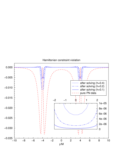
Figure 1: Hamiltonian constraint violation for a black hole separation of $r_{12}=8M$. The Hamiltonian constraint of pure PN data is much larger than the Hamiltonian constraint after solving (i.e. applying the the York procedure). We numerically solve for three different resolutions $h$. The inset is a blow up of the central region, which shows that our numerical scheme is second order convergent as expected.

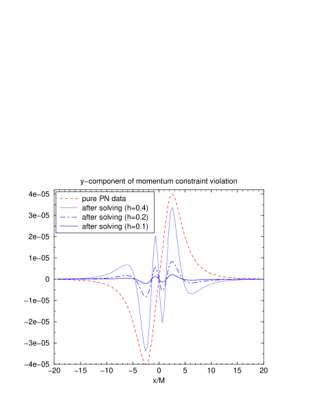
Figure 2: The momentum constraint for a separation of $r_{12}=8M$. We observe second order convergence in the resolution $h$ after solving. The momentum constraint violation of pure PN data is larger than after solving.

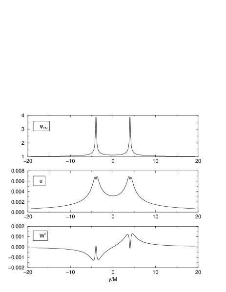
Figure 3: The solutions of $u$ and $W^{x}$ along the y-axis for a black hole separation of $r_{12}=8M$. For comparison we also show $\psi_{PN}$, which diverges at $y=\pm 4$.

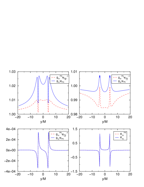
Figure 4: Components of the 3-metric and extrinsic curvature for a black hole separation of $r_{12}=8M$. The data are shown before (dashed lines) and after applying the York procedure (solid lines). The components of the 3-metric change on the order of $\sim 1\%$.

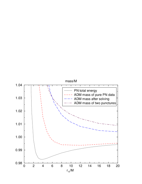
Figure 5: PN energy of Eq. (25) and ADM masses before and after solving (i.e. applying the York procedure) versus coordinate separation $r_{12}$ along the PN inspiral sequence. The data here were computed by keeping all momentum terms in $\psi_{PN}$, without consistently dropping higher order terms. In this case the ADM mass of pure PN data does not agree well with the PN energy. The ADM mass after solving (with $q=0.0$) increases on the order of $\sim 1\%$, when compared to the ADM mass of pure PN data. Furthermore the ADM mass after solving increases with decreasing separation, which is physically not acceptable. For comparison we also show the ADM mass of two puncture black holes along the PN sequence with constant bare masses, which show a similar increase in ADM mass.

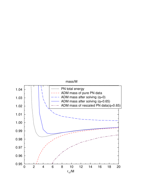
Figure 6: PN energy of Eq. (25) and ADM masses versus coordinate separation $r_{12}$ along the PN inspiral sequence. Shown are the ADM masses before and after applying the York procedure with both $q=0$ and $q=0.65$. Here all data are computed by consistently keeping momentum terms in $\psi_{PN}$ only up to Newtonian order. The ADM mass of pure PN data now agrees better with the PN energy. The York procedure with $q=0.0$ again increases the ADM mass on the order of $\sim 1\%$, when compared to the ADM mass of pure PN data. The ADM mass after solving with $q=0.65$, however, does not change very much and it also closely follows the PN energy down to $r_{12}\approx 6M$. Furthermore until $r_{12}\approx 5.6M$ it is physically reasonable since it decreases with decreasing separation. For comparison we also show the ADM mass curve of rescaled PN data (with $q=0.65$). These data, however, have no direct physical significance.

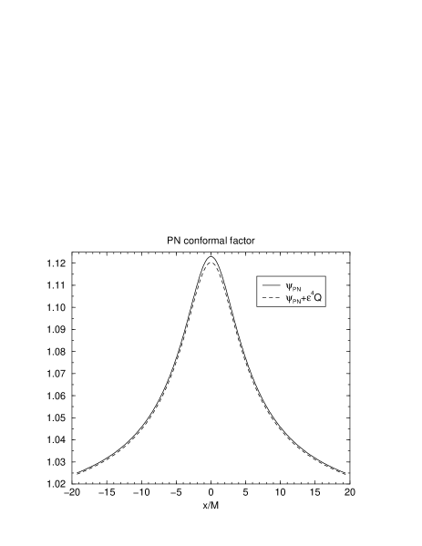
Figure 7: The conformal factors $\psi_{PN}$ and $\tilde{\psi}_{PN}=\psi_{PN}+\epsilon^{4}Q$, before and after rescaling with $q=0.65$ for $r_{12}=8M$. The difference between $\psi_{PN}$ and $\tilde{\psi}_{PN}$ is small.

For the numerical work in this paper we consider non-spinning equal mass binaries with their center of mass at rest at the origin. The binaries are in quasi-circular orbits in the sense that we use Eq. (24) to set the momentum of the two black holes before solving the constraints. The two black holes are on the y-axis, such that their momenta point in the positive and negative x-directions, resulting in an angular momentum along the z-direction. Fig. 1 shows the Hamiltonian constraint violation of pure PN data (dashed line), i.e. before solving the constraints, as well as the Hamiltonian constraint after solving at three different resolutions $h$. After the elliptic solve the constraint equations (44) and (49) are satisfied to within a given tolerance of $10^{-10}$ in the l2-norm, but to study convergence we show the ADM constraints computed from $g_{ij}$ and $K_{ij}$. The two black holes are at $y=\pm 4$. One can see that the constraint violation after the York procedure is much smaller than the constraint violation of pure PN data. The inset in Fig. 1 is a blow up of the center and shows second order convergence to zero in the Hamiltonian constraint after solving. We also observe second order convergence to zero in the momentum constraint. As an example we show the y-component of the momentum constraint in Fig. 2. We see that pure PN data violates the constraints. In Fig. 3 we plot the solutions $u$ and $W^{x}$ along the y-axis, which contains the black holes. As expected they are regular, unlike $\psi_{PN}$ which diverges at the black hole locations of $y=\pm 4$.

As expected, after applying the York procedure $g_{ij}$ and $K^{ij}$ are different from the pure PN expressions $g^{PN}_{ij}$ and $K_{PN}^{ij}$. Fig. 4 shows a comparison of several components of the 3-metrics $\psi_{PN}^{-4}g_{ij}$ and $\psi_{PN}^{-4}g^{PN}_{ij}$. As one can see, the components of $g_{ij}$ exhibit an increase on the order of $\sim 1\%$ when compared to $g^{PN}_{ij}$.

Table 1: Selected components of the 3-metric, extrinsic curvature and $h_{ij(4)}^{TT}$ at the point $x=0$, $y=12.2M$, $z=0$ for two black holes located on the y-axis at $y=\pm 5.2M$. The change in the 3-metric induced by solving the constraints without first rescaling $\psi_{PN}$ has about the same magnitude as the PN corrections at $O(\epsilon^{4})$. The data here are computed by inconsistently keeping all higher order momentum terms in $\psi_{PN}$.

PN value	Value after	relative
(up to $O(\epsilon^{5})$)	solving ($q=0$)	difference
$g^{PN}_{xx}=1.21866$	$g_{xx}=1.22285$	$\frac{g_{xx}-g^{PN}_{xx}}{g^{PN}_{xx}}=0.0034$
$K^{PN}_{xy}=-0.0022341$	$K_{xy}=-0.0022617$	$\frac{K_{xy}-K^{PN}_{xy}}{K^{PN}_{xy}}=-0.012$
PN metric	TT term in metric	relative size of
(up to $O(\epsilon^{5})$)	of $O(\epsilon^{4})$	$O(\epsilon^{4})$ correction
$g^{PN}_{xx}=1.21866$	$h_{xx(4)}^{TT}=0.00443$	$\frac{h_{xx(4)}^{TT}}{g^{PN}_{xx}}=0.0036$

The same conclusion is reached by looking at Tab. 1, which shows the 3-metric and extrinsic curvature before and after applying the York procedure. Furthermore Tab. 1 shows that the increase in the 3-metric due to applying the York procedure has about the same order of magnitude as the PN corrections at $O(\epsilon^{4})$. Since this happens in a region far enough from the particles that PN theory can actually be trusted to give realistic values, it means that solving the elliptic equations introduces significant differences between $g_{ij}$ and $g^{PN}_{ij}$ in the outer region due to changes in the inner region. Before we suggest how this problem can be addressed, let us also consider the ADM mass of the system, which is a coordinate invariant quantity.

We compute the ADM mass along PN inspiral sequences constructed from PN circular orbits with different radii. Along such a sequence the bare masses $m_{1}$ and $m_{2}$ are kept constant and the momenta are computed from Eq. (24) for circular orbits. Fig. 5 shows the numerically computed ADM mass of pure PN initial data (dashed line), the ADM mass of the data obtained after applying the York procedure (long dashed line), as well as the PN total energy (dotted line) of Eq. (25). In Fig. 5 and the following figures we plot data for $r_{12}$ between $1$ and $20M$. But note that it has to be expected that the PN data becomes inaccurate for small $r_{12}$, for example for $r_{12}\approx 4M$ where the black holes are close to the fiducial ISCO of the PN data.

In Fig. 5, we again observe an increase of $\sim 1\%$ in the ADM mass after applying the York procedure. A further problem is that none of the numerically determined ADM masses in Fig. 5 agrees very well with the PN energy (25). This problem stems from the fact that the PN initial data in Fig. 5 have been obtained by inserting the momentum (24) as it is into the expressions for 3-metric and extrinsic curvature of Sec. II without consistently dropping terms of $O(\epsilon^{6})$ or higher. Since all PN corrections to the momentum are positive, the main effect of this inconsistency is to increase $\psi_{PN}$ given by Eqs. (8) and (9). The result is that the numerically computed ADM masses before and after applying the York procedure show physically unacceptable behavior: (i) the ADM mass of pure PN data approaches the PN energy (25) only very slowly at large separations, and (ii) the ADM mass of the data after applying the York procedure monotonically increases with decreasing separation. This is physically not reasonable because the system is supposed to loose energy due to the emission of gravitational radiation. For reference the ADM mass (dot dashed line) for a sequence of two black hole punctures with constant bare masses and with the same PN momentum (24) is also shown in Fig. 5. Along this sequence the ADM mass of the punctures also unphysically rises with decreasing separation, which is not surprising since the assumption of constant bare masses for punctures ignores the growing contribution of $u$ to the conformal factor with decreasing separation of the punctures. In all cases studied by us the solution $u$ of Eq. (44) is indeed positive, which translates directly into an increase in the mass.

Of course, the question is how we can improve our data so that its behavior is physically more realistic. One can argue that part of the additional energy is tied to an increased local mass of the individual black holes. In fact, for constant bare masses there is a strong growth in the apparent horizon masses. A standard approach is therefore to rescale the bare masses to keep the apparent horizon mass fixed and to define a binding energy by subtracting the apparent horizon masses from the total mass, e.g. Cook (1994). We plan to compute apparent horizon masses for a future publication. However, in general it is not possible to unambiguously define a local mass for general relativistic data, and the accuracy and validity of the estimate for the binding energy therefore depends on, for example, how close the black holes are.

As an alternative we have experimented here with a mass correction that is tied to properties of the PN approximation. As a first step let us keep momentum terms of Eq. (24) in the PN conformal factor $\psi_{PN}$ (see Eqs. (8) and (9)) only up to the appropriate order and to consistently drop all terms of $O(\epsilon^{6})$ and higher. This amounts to just using the first Newtonian term of the momentum (24) in $\psi_{PN}$. The results are shown in Fig. 6. The ADM mass of pure PN data (dashed line) now much better approaches the PN energy for large separations. Yet, the ADM mass after simply applying the York procedure (long dashed line) still shows an increase of order $\sim 1\%$ when compared to pure PN data. If we want more physical mass curves we have to prevent this increase by preventing the increase in the conformal factor. We will take advantage of the freedom in the York procedure mentioned in Sec. IV.3 and use the conformal rescaling of Eq. (52) before applying the York procedure. From Eq. (55) we see that then the overall conformal factor becomes

$$\Psi=\tilde{\psi}_{PN}+u=\psi_{PN}+\epsilon^{4}Q+u.$$ (56)

Hence, if we choose an appropriate $Q$, we have a chance of compensating $u$ such that $\Psi\approx\psi_{PN}$ at least in the region far from the black holes where PN theory is valid.

Now, in the limit of $r_{12}\rightarrow\infty$ the pure PN data we use as a starting point represent two Schwarzschild black holes at rest (in isotropic coordinates). Thus $u$ is zero for infinite separation and we therefore expect that $u$ goes like $u\propto 1/r_{12}$ for large $r_{12}$. On the other hand we also have $u\propto 1/r$ so that we expect that $u$ is well approximated by

$$u\approx\frac{N}{r_{12}r}$$ (57)

for large $r$, where $N$ is some numerical constant. Since we want $Q+u\approx 0$, we choose

$$Q=-q\frac{m_{1}m_{2}}{2r_{12}}\left(\frac{1}{2r_{1}}+\frac{1}{2r_{2}}\right).$$ (58)

Here $q$ is a free parameter, which has to be chosen such that $Q+u\approx 0$ for large separations.

It turns out that for $q=0.65$ we get physically more reasonable mass curves in the regime where PN theory is expected to be valid. The solid line in Fig. 6 shows the ADM mass obtained for different separations if we apply the following extended York procedure: (i) start with the pure PN initial data, (ii) rescale $\psi_{PN}$ using Eqs. (55) and (58) with $q=0.65$ and (iii) apply the standard York procedure to the rescaled quantities. As we can see the ADM mass (solid line) closely follows the PN energy (dotted line) in the region where we expect PN theory to be valid. Furthermore for separations greater than $r_{12}\approx 5.6M$ the ADM mass decreases with decreasing separation as it should. For smaller separations the ADM mass again increases. In the literature this minimum has often been interpreted as the location of the innermost stable circular orbit (ISCO). Note, however, that the PN expressions which we used up to $O(\epsilon^{5})$ are probably close to breaking down around $M/r_{12}=1/5.6\approx 0.2$, so that the ISCO location may not be very accurate. Also the location of the minimum can be shifted if we use higher order terms in the rescaling of $\psi_{PN}$, i.e. if we use

$$\tilde{\psi}_{PN}=\psi_{PN}+\epsilon^{4}Q+\epsilon^{6}Q^{\prime}.$$ (59)

The extra $Q^{\prime}$ term will have no influence in the limit of large distances, but it will influence the mass curves at small separation and thus we can move the minimum. Again one could introduce a one-parameter family of $Q^{\prime}$ terms and fit the parameter such that the ADM mass curve has the minimum at the same place where the PN energy (25) has a minimum. We decided not to do this since the PN energy itself may not be very reliable near its minimum. For comparison, Fig. 6 also shows the ADM mass curve (dot dashed line) for the PN data rescaled by $Q$ with $q=0.65$, but without applying the York procedure. This curve has no direct physical meaning, but we can see that it can be obtained from the curve for pure PN data (dashed line) by a downwards shift. Fig. 7 shows the PN conformal factor before and after rescaling with $q=0.65$. We see that the change in $\psi_{PN}$ is rather small.

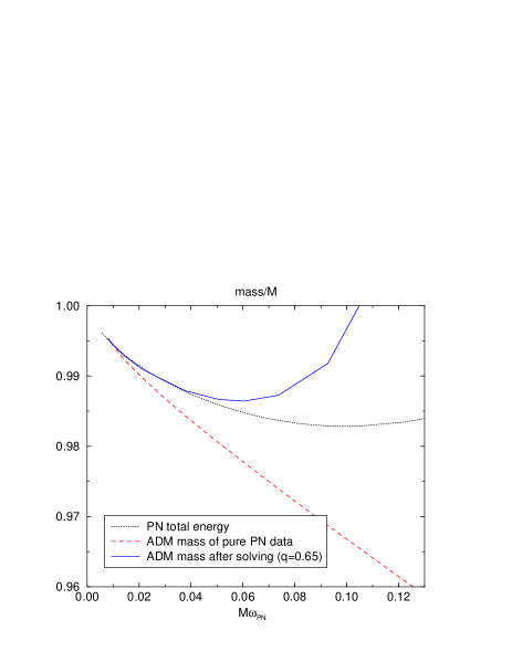
Figure 8: PN energy of Eq. (25), ADM mass of pure PN data and ADM mass after solving (with $q=0.65$) versus the PN angular velocity (60). The PN energy has a minimum near $M\omega_{PN}\approx 0.1$, which is often interpreted as the ISCO. We see that the ADM mass after solving (with $q=0.65$) closely follows the PN energy until $M\omega_{PN}\approx 0.05$. Then near $M\omega_{PN}\approx 0.06$ it has a minimum which could be regarded as the ISCO. One has to keep in mind, however, that the ambiguities in the York procedure in principle allow us to shift the location of this minimum.

All the masses so far are plotted versus the coordinate separation $r_{12}$. Fig. 8 shows the PN energy (dotted line), the ADM mass of pure PN data (dashed line) and the ADM mass of data obtained after rescaling with $q=0.65$ and applying the York procedure (solid line), versus the PN angular velocity $\omega_{PN}$, computed for circular orbits from

$$\left(M\omega_{PN}\right)^{2} = \frac{64(r_{12}/M)^{3}}{(1+2r_{12}/M)^{6}}+\frac{\mu}{M}\left(\frac{M}{r_{12}}\right)^{4}$$ (60)

$$+\left(-\frac{5}{8}\frac{\mu}{M}+\frac{\mu^{2}}{M^{2}}\right)\left(\frac{M}{r_{12}}\right)^{5}.$$

Note that $\omega_{PN}$ in Eq. (60) is written such that $\omega_{PN}$ is exact up to all PN orders in the limit of $\mu/M\rightarrow 0$. For $\mu/M>0$ Eq. (60) is accurate up to 2PN order. It should be kept in mind, however, that $\omega_{PN}$ probably is not exactly equal to the true angular velocity after applying the York procedure. Yet our numerical approach does not immediately yield an angular velocity which could be used in place of $\omega_{PN}$.

From Fig. 8 we see that the approximate ISCO of PN theory computed from the 2PN energy is near $M\omega_{PN}=0.1$, while the ISCO minimum of our data (after applying the extended York procedure with $q=0.65$) is near $M\omega_{PN}=0.06$, which is very close to the ISCO of test particles in Schwarzschild. Also note that the ADM mass of pure PN data (dashed line) does not have a minimum at all.

Table 2: Selected components of the 3-metric, extrinsic curvature and $h_{ij(4)}^{TT}$ at the point $x=0$, $y=12.2M$, $z=0$ for two black holes located on the y-axis at $y=\pm 5.2M$. The change in the 3-metric induced by solving the constraints after first rescaling $\psi_{PN}$ (with $q=0.65$) is much smaller than the the PN corrections at $O(\epsilon^{4})$. The change in the extrinsic curvature due to solving, however, does not depend much on $q$ and is about the same whether or not we use the rescaling with $q=0.65$. Here we have included only Newtonian momentum terms in $\psi_{PN}$, in order to have a consistent expansion in $\epsilon$.

PN value	Value after	relative
(up to $O(\epsilon^{5})$)	solving ($q=0.65$)	difference
$g^{PN}_{xx}=1.21738$	$g_{xx}=1.21783$	$\frac{g_{xx}-g^{PN}_{xx}}{g^{PN}_{xx}}=0.00037$
$K^{PN}_{xy}=-0.0022353$	$K_{xy}=-0.0022673$	$\frac{K_{xy}-K^{PN}_{xy}}{K^{PN}_{xy}}=-0.014$
PN metric	TT term in metric	relative size of
(up to $O(\epsilon^{5})$)	of $O(\epsilon^{4})$	$O(\epsilon^{4})$ correction
$g^{PN}_{xx}=1.21738$	$h_{xx(4)}^{TT}=0.00443$	$\frac{h_{xx(4)}^{TT}}{g^{PN}_{xx}}=0.00364$

In Tab. 2 we compare some components of the 3-metric and extrinsic curvature of pure PN data with the corresponding quantities obtained after rescaling with $q=0.65$ and applying the York procedure. The change in the 3-metric induced by solving the constraints after first correcting $\psi_{PN}$ (with $q=0.65$) now is much smaller than the the PN corrections at $O(\epsilon^{4})$. The change in the extrinsic curvature due to solving, however, is nearly the same whether or not we use the rescaling with $q=0.65$.

The question arises if the solutions $g_{ij}$ and $K^{ij}$ with $q=0.65$ are astrophysically more realistic then the pure PN solutions $g^{PN}_{ij}$ and $K_{PN}^{ij}$. We argue that this is indeed the case since $g_{ij}$ and $K^{ij}$ with $q=0.65$ are close to $g^{PN}_{ij}$ and $K_{PN}^{ij}$ in the far region where PN is accurate, but in addition do fulfill the constraint equations of general relativity. Furthermore the ADM mass curve for $g_{ij}$ and $K^{ij}$ with $q=0.65$ is closer to the PN energy (25) than the ADM mass curve of the pure PN solutions $g^{PN}_{ij}$ and $K_{PN}^{ij}$.

VI Discussion

For the first time, we have derived fully relativistic black hole initial data for numerical relativity, starting from 2PN expressions of the 3-metric and extrinsic curvature in the ADMTT gauge. We have used the York procedure, and any procedure for projecting the PN data onto the solution manifold of general relativity will introduce changes to the PN data. The larger the violation of the constraints by the PN data, the larger the change in the solution process will be. In principle one may loose the PN characteristics that distinguished the PN data from other approaches in the first place.

As we have seen in Sec. V, the size of these changes depends on how exactly we employ the York procedure for the projection. We find that the extended York procedure (with $q=0.65$) yields acceptably small changes, so that if the PN data we started with are astrophysically realistic, the data after solving the constraints should still be astrophysically relevant. In particular, our new PN initial data have the nice property that the 3-metric and extrinsic curvature approach the corresponding 2PN expressions in the region where PN theory is valid, providing a natural link to the early inspiral phase of the binary system. Furthermore, our approach leads to an easy numerical implementation with a generalized puncture method.

We consider this work as a first step towards the construction of astrophysical initial data based on the PN approximation. Although we are able to remove some of the inherent ambiguity of the method, several directions should be explored. Since the PN formalism is unable to unambiguously provide the full information in the black hole region, one should examine different ways to introduce black holes. Furthermore it would seem natural to follow the conformal thin sandwich approach in order to obtain data that corresponds more closely to a quasi-equilibrium configuration, although in principle we rather want data for the appropriate PN inspiral rate than for exactly circular orbits. Note that after the solution process it is not known how well the orbital parameters correspond to quasi-circular orbits. One could use, for example, the effective potential method Cook (1994) with the new PN based data to determine quasi-circular orbits of the two black holes.

Another direction of research is to improve the PN input to our method. Even though we can solve the constraints for rather small separations of the black holes, we cannot trust the numerical data for arbitrarily small coordinate separation, because this is where the PN data we start with is probably unreliable. We have started with a traditional PN approach Jaranowski and Schäfer (1998), but there has been significant progress in extending the validity of the PN approximation to smaller separations through resummation techniques Buonanno and Damour (2000); Damour et al. (1998, 2001b). It is an important issue to study how large an intermediate binary black hole regime might be, where the PN approximation has broken down but the separation is still significantly larger than the separation for an approximate ISCO Brady et al. (1998).

In addition, we want to work with higher order PN approximations. The explicit regularization for 3PN of Damour et al. (2001a) could be used as a starting point. However, our procedure may have to be modified because of changes in the conformal factor $\psi_{PN}$. Finally, Jaranowski and Schäfer Jaranowski and Schäfer have recently provided us with an expression which includes spin terms at order $(v/c)^{3}$ in the PN extrinsic curvature. In future work we intend to use these terms to add spin to the black holes.

Recall that we have concentrated on the near zone. We plan to replace the near zone expansion of $h_{ij(4)}^{TT}$ with a globally valid expression. This could be achieved by solving the wave equation determining $h_{ij(4)}^{TT}$ (see e.g. Schäfer (1986)) numerically, without any near zone approximations, which would be natural in a method that resorts to numerics anyway. If the PN inspiral trajectory is used in this calculation, the initial slice of our spacetime will already contain realistic gravitational waves, with the correct PN phasing. When this spacetime is then evolved numerically we might eventually be able to compute numerical wave forms which continuously match PN wave forms.

This brings us to the final goal of our initial data construction, namely to use it as the starting point for numerical evolutions. As we pointed out in the introduction, there are now numerical evolution methods with which we can begin to explore the physical content of any initial data set by evolution and by extraction of physical quantities such as detailed wave forms or total radiated energies Alcubierre et al. (2001, 2002); Baker et al. (2002a). As mentioned in Baker et al. (2002a), the Lazarus approach provides an effective method for cross-checking the validity of the results by choosing different transition times along the binary orbit in the region where a far limit approximation (such as the PN method) and full numerical relativity overlap. Only by extending the ability of full numerical codes to accurately compute several orbits, will we be able to arrive at a definitive conclusion about the merit of different initial data sets.