Early radiative properties of the developments of time symmetric, conformally flat initial data

Abstract

Using a representation of spatial infinity based in the properties of conformal geodesics, the first terms of an expansion for the Bondi mass for the development of time symmetric, conformally flat initial data are calculated. As it is to be expected, the Bondi mass agrees with the ADM at the sets where null infinity “touches” spatial infinity. The second term in the expansion is proportional to the sum of the squared norms of the Newman-Penrose constants of the spacetime. In base of this result it is argued that these constants may provide a measure of the incoming radiation contained in the spacetime. This is illustrated by means of the Misner and Brill-Lindquist data sets.

Introduction. The study of the radiative properties of dynamical spacetimes describing isolated systems adquires these days more relevance in view of the beginning of operations of several interferometric gravitational wave detectors (LIGO, GEO 600). One of the crucial radiative properties to be analysed is the mass loss due to the radiative processes. Strictly speaking, the radiative properties are global features of the spacetimes, and thus they can only be unambiguosly defined at infinity. Penrose Penrose (1963) has put forward the idea of the description of spacetimes describing isolated system by means of an unphysical spacetime $(M,g_{\mu\nu})$ obtained from the original (physical) spacetime $(\widetilde{M},\widetilde{g}_{\mu\nu})$ through a conformal rescaling: $g_{\mu\nu}=\Theta^{2}\widetilde{g}_{\mu\nu}$. It is within this framework that notions like the mass loss due to radiative processes can be rigorously defined. The mass loss notion is captured in the form of the Bondi mass which is given as the integral Penrose and Rindler (1986),

$$m_{B}=-\frac{1}{4\pi}\oint\left(\psi_{2}^{0}-\sigma_{0}\dot{\overline{\sigma}}_{0}\right)dS,$$ (1)

over cuts of null infinity. The functions $\psi_{2}^{0}$ and $\sigma_{0}$ are the leading terms in of the component $\widetilde{\psi_{2}}$ ($\mathcal{O}(\Theta^{3})$)of the Weyl tensor and the Newman-Penrose spin coefficient $\widetilde{\sigma}$ ($\mathcal{O}(\Theta^{2})$) respectively in a so-called Bondi system.

To the author’s knowledge, the formula (1) has never been evaluated on a realistic spacetime. Furthermore, the dependence of the Bondi mass on the initial data (assuming that the spacetime arises as the development of some suitable Cauchy data) whose development gives rise to (weakly) asymptotically simple spacetimes has never been analysed. It is the purpose of this letter to show that by means of the conformal field equations and an adequate gauge choice it is possible to obtain expansions of the gravitational field in which the dependence on initial data can be read directly. In particular, this approach enables us to calculate an expansion for the Bondi mass which shows a remarkable, yet misterious, connection with another global property of the spacetime: the Newman-Penrose constants —see equation (13). Our analysis will be restricted to time symmetric, conformally flat initial data.

Spacetime close to spatial infinity. The natural arena for a discussion of the early radiative properties of spacetime is the neighbourhood of $i^{0}$ and ${I}^{+}$. In particular, it has been shown that under by fiat assumptions that the Bondi mass tends to the ADM mass as one approaches spatial infinity along future null infinity Ashtekar and Magnon-Ashtekar (1979). In order to discuss the properties of spacetime in this region, one would like to make use of the Friedrich conformal field equations. These provide a regular system of partial differential equations for the field quantities in the unphysical spacetime. However, in the way they were first given (see for example Friedrich (1983)) they are not too well suited for an analysis near spatial infinity. It can be shown that for the Weyl tensor one has $\psi_{abcd}=\mathcal{O}(m/\rho^{3})$, where $\rho$ is a geodesic distance to spatial infinity on an initial Cauchy hypersurface $S$, and $m$ is the ADM mass. Thus, the standard representation of spatial infinity as a point (see figure 1) is too narrow to discuss fully the consequences of the conformal field equations.

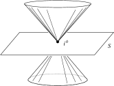
Figure 1: The standard representation of spacetime in the neighbourhood of spatial infinity. Spacetime corresponds to the region outside the cone.

Using a extended version Friedrich (1995) of the conformal field equations which allows to consider Weyl connections and a gauge based on the properties of conformal geodesics, it is possible to arrive to a new representation of spatial infinity which allows to formulate an initial value problem in the neighbourhood of spatial infinity such that: (i) the equations and initial data are regular, (ii) the location of null infinity is known a priori via a conformal factor $\Theta$ that can be read-off from the initial data once the constraint equations have been solved Friedrich (1998). The unknowns in this setting are the frame ($c^{\mu}_{ab}$, $\mu=0,\dots,3$), the connection ($\Gamma_{abcd}$), the Ricci curvature ($\Theta_{abcd}$) and the Weyl curvature ($\phi_{abcd}$) of the unphysical spacetime, $a,b,c,d=0,1$ being spinorial indices. In this conformal geodesic gauge representation of spatial infinity, the point $i^{0}$ is blown up to obtain a cylinder $I=S^{2}\times(-1,1)=\{\rho=0,|\tau|<1\}$ (see figure 2). The sets $I^{\pm}=\{\rho=0,\tau=\pm 1\}$ where null infinity touches spatial infinity are of a special nature and will be further discussed later.

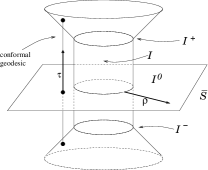
Figure 2: The cylinder at spatial infinity. Again, spacetime corresponds to the region outside the cones and the cylinder.

In the gauge given by the conformal geodesics, the equations for the unknowns $v=(c^{\mu}_{ab},\Gamma_{abcd},\Theta_{abcd})$ are of the form:

$$\partial_{\tau}v=Kv+Q(v,v)+L\phi,$$ (2)

where $K$, $Q$ denote respectively linear and quadratic functions with constant coefficients, and $L$ denotes a linear function with coefficients depending on the coordinates and such that $L|_{I}=0$. Differentiating formally with respect to $\rho$ $p$ times and evaluating on $I$ one obtains,

$$\partial_{\tau}v^{(p)}=Kv^{(p)}+Q(v^{(0)},v^{(p)})+Q(v^{(p)},v^{(0)})$$

$$+\sum_{j=1}^{p-1}\left(Q(v^{(j)},v^{(p-j)})+L^{(j)}\phi^{(p-j)}\right)+L^{(p)}\phi^{(0)},$$ (3)

where ^(p) denotes the operation of taking the $p$-th derivative with respect to $\rho$ and evaluating at $\rho=0$, and $\phi=(\phi_{0},\phi_{1},\phi_{2},\phi_{3},\phi_{4})$. $L^{(p)}\neq 0$ for $p\geq 1$. The equations for the components of the Weyl tensor are slightly more complicated,

$$A^{\mu}\partial_{\mu}\phi=B(\Gamma)\phi,$$ (4)

where $A^{\mu}$, $\mu=0,\ldots,3$ are $5\times 5$ matrices depending on $c^{\mu}_{ab}$ such that,

$$A^{0}|_{I}=\sqrt{2}\mbox{diag}(1+\tau,1,1,1,1-\tau),\qquad A^{1}|_{I}=0,$$ (5)

and $B(\Gamma)$ is a matrix value function of the connection coefficients. From the second equality one sees that the $\rho$ derivatives disappear from the field equations upon evaluation on $I$. Therefore, we call $I$ a total characteristic of the system (2)-(4). Differentiating formally with respect to $\rho$ $p$ times and evaluating on $I$ one obtains,

$$A^{0}\partial_{\tau}\phi^{(p)}+A^{C}\partial_{C}\phi^{(p)}=B(\Gamma^{(0)}_{abcd})\phi^{(p)}$$

$$+\sum_{j=1}^{p}\left(\begin{array}[]{c}p\\ j\end{array}\right)\left\{B(\Gamma^{(j)}_{abcd})\phi^{(p-j)}-(A^{\mu})^{(j)}\partial_{\mu}\phi^{(p-j)}\right\},$$ (8)

where $C=2,3$. The system composed by (Early radiative properties of the developments of time symmetric, conformally flat initial data) and (Early radiative properties of the developments of time symmetric, conformally flat initial data) for a fixed $p$ are called the transport equations of order $p$ on the cylinder at spatial infinity. The transport equations allow us to obtain expansions for the field equations of the form,

$$u=\sum\frac{1}{p!}u^{(p)}\rho^{p},$$ (9)

where $u^{(p)}=u^{(p)}(\tau,x^{C})$. In the case of time symmetric initial data, the solutions of the system (Early radiative properties of the developments of time symmetric, conformally flat initial data) with $p=0$ coincide with the $p=0$ solutions of Minkowski spacetime. For $p\geq 1$, the equations are linear. The equations (Early radiative properties of the developments of time symmetric, conformally flat initial data) are essentially ode’s which allow us to calculate $v^{(p)}$ if $u^{(k)}$ for $0\leq k<p$ are known. Once this has been done, one can calculate $\phi^{(p)}$. Note however, that because of the first equality in (5), the system (Early radiative properties of the developments of time symmetric, conformally flat initial data) is singular at the sets $I^{\pm}=\{\rho=0,\tau=\pm 1\}$ where null infinity “touches”spatial infinity. This phenomenon can be understood by recalling that while ${I}$ is a characteristic of the conformal field equations, $I$ is a total characteristic. Thus, a degeneracy occurs at $I^{\pm}$.

In Friedrich (1998) a first analysis of the properties of the transport equations under the assumption of time symmetry of the initial data (i.e. vanishing extrinsic curvature of the initial hypersurface) was carried out. It is found that a necessary condition for the transport equations to have smooth solutions at the sets $I^{\pm}$ is,

$$D_{(a_{s}b_{s}\cdots}D_{a_{1}b_{1}}b_{abcd)}(i^{0})=0,\quad s=0,1,\dots\;\;,$$ (10)

where $D_{ab}$ denotes covariant derivatives with respect to the initial 3-metric, and $b_{abcd}$ is the Cotton-Bach spinor. The vanishing of the Cotton-Bach spinor characterises locally conformally flat initial data. If the regularity condition (10) does not hold for a certain $p$ it can be seen that the transport equations develop logarithmic singularities at $I^{\pm}$. It is conjectured that the regularity condition is also a sufficient condition for the solutions of the transport equations with time symmetric initial data to be smooth at $I^{\pm}$. This however remains to be proved. The generalisation of the condition (10) for non-time symmetric is also unknown. The importance of the transport equations (Early radiative properties of the developments of time symmetric, conformally flat initial data) and (Early radiative properties of the developments of time symmetric, conformally flat initial data) lies in the fact that they allow us to relate directly quantities defined on ${I}$ —the Bondi mass in particular— with the initial data from which the asymptotically simple spacetime arises.

Conformally flat initial data. The regularity condition (10) is satisfied in a trivial way for time symmetric, conformally flat initial data. This fact allow us to conjecture that the developments of this class of initial data are candidates for spacetimes with a smooth null infinity. Conformally flat initial data are of great interest as all the time symmetric initial data sets for head-on black hole collisions currently in use in numerical simulations are of this type. We will restrict the following discussion to them. Being time symmetric, the initial 3-geometries we want to consider are completely described in terms of the following line element,

$$ds^{2}=-\chi^{4}\;ds^{2}_{flat},$$ (11)

with $\chi$ satisfying the Laplace equation. It is customary to write, $\chi=1+\rho W$, where $\rho$ is the geodesic distance from $i$. From the Yamabe equation one has that,

$$W=\frac{m}{2}+\sum_{p=1}^{\infty}\sum_{k=-p}^{p}\frac{1}{p!}w_{p,2p,n-k}i^{2n-m}\sqrt{\frac{4\pi}{2n+1}}Y_{n,m}\rho^{p},$$ (12)

where $m$ is the total (ADM) mass, and $w_{p,2p,n-k}$ are complex constants satisfying the reality condition $\overline{w}_{p,2p,2p-k}=w_{p,2p,k}$. The functions $Y_{n,m}$ are the standard spherical harmonics. Although the system of transport equations is of large size ($50\times 50$), its properties make it quite amenable to a treatment by means of a computer algebra system. A series of scripts in the computer algebra system Maple V have been written in order to solve the transport equations (Early radiative properties of the developments of time symmetric, conformally flat initial data) and (Early radiative properties of the developments of time symmetric, conformally flat initial data) up to $p=5$ for time symmetric conformally flat initial data. The solutions of the transport equations up to this order are polynomial. This is in itself an outstanding feature, and it is believed to occur at all higher orders. Yet a proof of this fact lies far in the future. This adds further support to the conjecture that time symmetric, conformally flat initial data sets yield developments with a smooth null infinity. The details of the implementation of the transport equation solver and the detailed structure of the solutions for generic time symmetric initial data will be presented elsewhere. It should be pointed out that the transport equations are extremely sensitive to any small change in their structure. Any change would inmediately give rise to non-smooth solutions containing logarithms. The absense of such kind of solutions in the expansions up to order $p=5$ is in itself a guarantee of the correctness of our results.

Calculating the Bondi mass near spatial infinity. A natural application of the expansions is to calculate the first orders of the Bondi mass in aregion of ${I}$ close to spatial infinity. The formula (1) cannot be used directly as it stands for it is given in the so-called Bondi gauge, while the gauge used in the representation of spatial infinity is based in the properties of conformal geodesics. The connection between the two gauges has been given in Friedrich and Kánnár (2000). Knowledge of the solutions to the transport equations up to $p=5$ order permits the calculation of the first 2 terms of the expansion for the Bondi mass. A lengthy calculation yields,

$$m_{B}=m+\sum_{k=-2}^{2}|G_{k}|^{2}\left(\frac{\sqrt{2}}{u}\right)^{7}+O(\rho^{8}),$$ (13)

where $u$ is a standard Bondi retarded time ($u\rightarrow-\infty$ as one approaches to $I^{+}$) and,

$$G_{-2}=-\textstyle\frac{\sqrt{6}}{4}\left(mw_{2;4,4}-2\sqrt{6}w_{1;2,2}^{2}\right),$$

$$G_{-1}=-\textstyle\frac{\sqrt{6}}{4}\left(mw_{2;4,3}-2\sqrt{12}w_{1;2,2}w_{1;2,1}\right),$$

$$G_{0}=-\textstyle\frac{\sqrt{6}}{4}\left(mw_{2;4,2}-4(w_{1;2,0}w_{1;2,2}+w_{1;2,1}^{2})\right),$$

$$G_{1}=-\textstyle\frac{\sqrt{6}}{4}\left(mw_{2;4,1}-2\sqrt{12}w_{1;2,0}w_{1;2,1}\right),$$

$$G_{2}=-\textstyle\frac{\sqrt{6}}{4}\left(mw_{2;4,0}-2\sqrt{6}w_{1;2,0}^{2}\right),$$

are, up to an irrelevant numerical factor, the Newman-Penrose (NP) constants Newman and Penrose (1965) of the development expressed in terms of the initial data as given by Friedrich and Kánnár. Note that close to $I^{+}$ the second term in (13) is negative, in agreement with the fact that the Bondi mass is non-increasing. The formula (13) is rather unexpected. Before having performed the calculation, there was principle, no reason for this to be the case. This evidenciates the power conveyed in our approach, and the kind of information that it is possible to extract through it. The NP constants are defined as integrals over cuts of ${I}^{+}$ of the derivative with respect of a parameter of the generators of light cones escaping to null infinity of the $\psi_{0}$ component of the Weyl tensor. They are absolutely conserved in the sense that they have the same value for any cut of ${I}^{+}$. For spacetimes admitting a conformal compactification that includes the point $i^{+}$ (future time infinity), the NP constants are equal to the value of the Weyl tensor precisely at $i^{+}$ Newman and Penrose (1968); Friedrich and Schmidt (1987). Thus, the NP constants contain global information of the spacetime that can be read directly from the initial data! The NP constants have also been found playing a role in determining the decay rate of self-gravitating waves in a Schwarzschild background Gómez et al. (1994):waves with vanishing NP constants are found to decay faster. On the same lines, an analysis of some particular boost-rotation symmetric solutions near $i^{+}$ has shown, remarkably, that the squared norm of the NP constants appear again in the leading term of the time derivative of the Bondi mass (late radiated power) Lazkoz and Valiente-Kroon (2000). There has been some discussion concerning the idea of the NP giving a measure of the spurious radiation contained in the spacetime in general, and via formula (13) on the initial Cauchy hypersurface in particular. The idea being that the first radiation reaching ${I}^{+}$ as the system begins to evolve can not be truthly attributed to the processes occurring in the interior of the spacetime (a black hole collision, for example) as it requires some time to reach the asymptotic region. Formula (13) is local, and thus valid for an arbitrarily small neighbourhood of spatial infinity. It will register radiation that is already in the asymptotic region and that had to be put in in order to construct the initial data. Note that formula (13) implies that the NP constants of static spacetimes (the Schwarzschild solution in particular) arising from conformally flat data must vanish. This latter fact can also be independently verified using the Friedrich-Kánnár formula for the NP constants on static initial data. Similarly, the recent examples of non-trivial asymptotically simple spacetimes given by Chruściel and Delay Chruściel and Delay (2002) have also vanishing NP constants, and accordingly a very special radiation content.

The formula (13) has only been calculated for developments of time symmetric, conformally flat initial data sets. It is expected that a similar result would hold (modulo some more involved calculations) for general time symmetric data. For initial data with non-vanishing second fundamental form the situation is less clear. The study expansions of the gravitational field obtained from the transport equations (Early radiative properties of the developments of time symmetric, conformally flat initial data) and (Early radiative properties of the developments of time symmetric, conformally flat initial data) were first carried with the purpose of laying the first steps towards a global existence proof of non-trivial spacetimes with a smooth structure at null infinity in general, and the verification of the conjecture regarding the regularity condition (10) in particular. However, as (13) evidenciates they also happen to be a powerful tool in order to discuss the physics contained in these spacetimes.

Comparing the Misner and Brill-Lindquist initial data sets. As an application of our result, one can perform a comparison of the NP constants of the development of physically equivalent Brill-Lindquist (BL) and Misner initial data. The interest of this example lies in the fact that both initial data sets provide a model to describe head on black hole collisions. Both initial data sets are time symmetric, conformally flat, and the crucial difference between each other lies in their topology: 3 asymptotically flat regions connected by 2 throats in the BL case, and 2 asymptotically flat regions connected by 2 throats in the Misner case. For physically equivalent BL and Misner data sets it is understood data sets such that: (1) the ADM mass of the initial hypersurface measured at the reference asymptotic end is the same; and (2) the geodesic separation of the innermost minimal surfaces is the same. For the case of the Misner data, there is an explicit formula for the separation of the minimal surfaces, while for the BL data it has to be calculated numerically. Čadež Čadež (1974) has given a tabulation of the values of this distance for different values of the parameters of the BL initial data.

Figure 3: The Newman-Penrose constants for physically equivalent Misner and Brill-Lindquist initial data sets.

Due to the axial symmetry of the Misner and BL initial data sets, there is only one non-vanishing NP constant for each one of the developments ($G_{2}$). An analysis of the NP constants for the BL data has been recently given in Dain and Valiente Kroon (2002). The function $W$ —see formula (12)— for the BL data has been calculated there. The one for the Misner data can be calculated in a similar fashion. A plot of the values of the constant for various physically equivalent initial data sets is shown in figure 3. It can be seen that for black holes initially very separated the difference between the NP constants of the two topologically different initial data set is negligible, and it increases as one considers data sets where the separation is smaller. For black holes separated a distance of $L\approx 5.26(m/2)$ where $m$ is the total ADM mass of the spacetime one has $|G_{2(BL)}|^{2}/|G_{2_{(}Misner)}|^{2}\approx 0.66$. The physical content of this difference, and the possibility of interpreting it as some measure of the (spurious) radiation contained in the initial data sets is certainly a matter of debate.

Acknowledgements. I would like to thank H. Friedrich, S. Dain, J. Winicour and M. Mars for several discussions.

References

- Penrose (1963) R. Penrose, Phys. Rev. Lett. 10, 66 (1963).
- Penrose and Rindler (1986) R. Penrose and W. Rindler, Spinors and space-time. Volume 2. Spinor and twistor methods in space-time geometry (Cambridge University Press, 1986).
- Ashtekar and Magnon-Ashtekar (1979) A. Ashtekar and A. Magnon-Ashtekar, Phys. Rev. Lett. 43, 181 (1979).
- Friedrich (1983) H. Friedrich, Comm. Math. Phys. 91, 445 (1983).
- Friedrich (1995) H. Friedrich, J. Geom. Phys. 17, 125 (1995).
- Friedrich (1998) H. Friedrich, J. Geom. Phys. 24, 83 (1998).
- Friedrich and Kánnár (2000) H. Friedrich and J. Kánnár, J. Math. Phys. 41, 2195 (2000).
- Newman and Penrose (1965) E. T. Newman and R. Penrose, Phys. Rev. Lett. 15, 231 (1965).
- Newman and Penrose (1968) E. T. Newman and R. Penrose, Proc. Roy. Soc. Lond. A 305, 175 (1968).
- Friedrich and Schmidt (1987) H. Friedrich and B. Schmidt, Proc. Roy. Soc. Lond. A 414, 171 (1987).
- Gómez et al. (1994) R. Gómez, J. Winicour, and B. G. Schmidt, Phys. Rev. D 49, 2828 (1994).
- Lazkoz and Valiente-Kroon (2000) R. Lazkoz and J. A. Valiente-Kroon, Phys. Rev. D 62, 084033 (2000).
- Chruściel and Delay (2002) P. T. Chruściel and E. Delay, Class. Quantum Grav. 19, L71 (2002).
- Čadež (1974) A. Čadež, Ann. Phys. 83, 449 (1974).
- Dain and Valiente Kroon (2002) S. Dain and J. A. Valiente Kroon, Class. Quantum Grav. 19, 811 (2002).