Abstract

Topological solutions in the (2+1)-dimensional Einstein theory of gravity are studied within the ADM canonical formalism. It is found that a conical singularity appears in the closed de Sitter universe solution as a topological defect in the case of the Einstein theory with a cosmological constant. Quantum effects on the conical singularity are studied using the de Broglie-Bohm interpretation. Finite quantum tunneling effects are obtained for the closed de Sitter universe, while no quantum effects are obtained for an open universe.

1 Introduction

A quantum theory of gravity is required to unify the four fundamental interactions and to reduce the singular behavior of the early universe and of the central region of black holes. Superstring theory [1] and M-theory [2] are very promising approaches but the analysis of these theories have not yet been completed, because non-perturbative effects are difficult to evaluate. Recently, the interesting correspondence between the gravity theory in (d+1)-dimensional anti-de Sitter space (AdS) and the conformal field theory (CFT) in d-dimensions has been elucidated using the concept of duality in the superstring theory [3]. The microscopic derivation of the black hole entropy has also been studied extensively to apply the AdS/CFT correspondence [4].

In several works of particular interest, it has been shown that the Einstein theory of gravity in (2+1)-dimensional anti-de Sitter space is equivalent to the Chern-Simons gauge theory [5, 6], while black hole entropy has been studied in terms of its asymptotic symmetry [7, 8, 9, 10, 11]. The (2+1)-dimensional gravity theory is a simple toy model that possesses no local or physical modes (like gravitational wave modes), but it does possess interesting global and topological modes.

A conical singularity is one of the charasteristic features of the (2+1)-dimensional gravity theory [12]. In the case of a point particle with mass $m_{0}$ located at the origin of the spatial coordinates, we consider a static spherically symmetric metric of the form

$$ds^{2}=-dt^{2}+{\rm e}^{\sigma(r)}(dr^{2}+r^{2}d\phi^{2})\ .$$ (1)

In this case, the Einstein equation becomes

$$\bigtriangleup\sigma=m_{0}\delta^{(2)}(\vec{r})\ ,$$ (2)

and we obtain its solution as

$$ds^{2}=-dt^{2}+r^{-8m_{0}G}(dr^{2}+r^{2}d\phi^{2})\;,$$ (3)

where the ranges of the variables are given by $0\leq r<\infty$ and $\ 0\leq\phi<2\pi$. In order to transform to a flat metric, we make a change of variables $r\rightarrow\overline{r}$ ,$\phi\rightarrow\overline{\phi}$, defined by the following:

$$\bar{r} = r^{1-4m_{0}G}/(1-4m_{0}G)\;,$$ (4)

$$\bar{\phi} = (1-4m_{0}G)\phi\;,$$ (5)

$$ds^{2} = -dt^{2}+\bar{d}\bar{r}^{2}+\bar{r}^{2}d\bar{\phi}^{2}\;.$$ (6)

The ranges of the variables $\overline{r}$ and $\overline{\phi}$ become $0\leq\bar{r}<\infty$ and $0\leq\bar{\phi}<2\pi-8\pi m_{0}G$. Here the deficit angle $8\pi m_{0}G$ appears, and this leads to a conical singularity (see Fig.1).

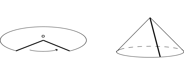
Figure 1: (A) The deficit angle $8\pi m_{0}G=2\pi m_{0}$ is shown. (B) The conical singularity is formed gluing edges of the deficit angle shown in (A).

In this paper, we study the (2+1)-dimensional Einstein gravity theory with a cosmological constant within the framework of the traditional canonical formalism [13, 14]. We quantize the theory in order that the constraint operators form a closed algebra. We obtain quantum de Sitter universe solutions applying the dBB interpretation and rederive the known classical de Sitter universe solutions as the classical limits.

The dBB interpretation is a natural extension of the WKB approach (i.e., the semi-classical method) into the full quantum region [16]. In this interpretation, the wave function in polar coordinates, $\Psi=\mid\Psi\mid{\rm e}^{i\Theta}$ is understood with the following meaning: (a) the amplitude squared $\mid\Psi\mid^{2}$ is consedered the probability distribution of metrics, and (b) the momenta are defined by the gradient of the phase according to

$$\frac{\partial\Theta}{\partial({\rm metric})}=({\rm momentum})\ .$$ (7)

We call this the de Broglie-Bohm (dBB) equation. The dBB interpretation has the following advantageous features in the quantum gravity theory: (i) A metric including quantum effects can be obtained from the dBB equation (7); (ii) a kind of time is introduced through the dBB equation [17], which is lost in the constraint equations [see Eq. (24) in Section 2]; (iii) neither an outside observer nor a measurement is necessary to realize the classical universe from the quantum universe asymptotically.

This paper is organized as follows. In Section 2, we review the canonical quantization of the Einstein theory of gravity in (2+1) dimensions and apply the dBB interpretation to the wave function. The notation and our basic idea follow those of Kuchař’s work [18] and our previous paper [19]. In Section 3, we study the conical singularity of the closed de Sitter universe solution. This solution is interesting with regard to two points: (1) the correlation between local objects (black holes) and the global object (the de Sitter universe) and (2) quantum effects on the systems as implied by the de Broglie-Bohm interpretation. A summary of the paper is given in Section 4.

2 Quantum Solutions and the De Broglie-Bohm Interpretation

We start from the Einstein-Hilbert action with a cosmological constant $\lambda$ in (2+1)-dimensional spacetime,

$$I=\frac{1}{4\pi}\int d^{3}x\,\sqrt{-{\rm det}g}\,(R-2\lambda)\;,$$ (8)

where the gravitational constant is set to $G_{2}={1/4}$. We write the metric of the general spherically symmetric spacetime in the (2+1) decomposition [14, 18, 19] as

$$ds^{2}=-(N^{t})^{2}dt^{2} + \Lambda^{2}(dr+N^{r}dt)^{2}+R^{2}(d\phi+N^{\phi}dt)^{2}$$ (9)

$$+ 2C(dr+N^{r}dt)(d\phi+N^{\phi}dt)\ ,$$

where the metric is a function of $r$ and $t$.

The action in the canonical formalism is written in the form

$$I=\int dtdr(P_{\Lambda}\dot{\Lambda}+P_{R}\dot{R}+P_{C}\dot{C}-N^{t}H_{t}-N^{r}H_{r}-N^{\phi}H_{\phi})\;,$$ (10)

where $P_{\Lambda},P_{R}$ and $P_{C}$ are the canonical momenta,

$$P_{\Lambda} = \frac{\Lambda R(N^{r}R^{\prime}-\dot{R})}{N^{t}\sqrt{h}}\ ,\$$ (11)

$$P_{R} = \frac{R[C(N^{\phi})^{\prime}+\Lambda((\Lambda N^{r})^{\prime}-\dot{\Lambda})]}{N^{t}\sqrt{h}}\ ,\$$ (12)

$$P_{C} = -\frac{(N^{r}C)^{\prime}+R^{2}(N^{\phi})^{\prime}-\dot{C}}{2N^{t}\sqrt{h}}\ ,$$ (13)

where

$$h=R^{2}\Lambda^{2}-C^{2}\ .$$ (14)

In the above, the dot and prime denote the differentiation with respect to $t$ and $r$, respectively. The coefficients of the auxiliary metrics $N^{t},N^{r}$ and $N^{\phi}$ are the Hamiltonian $H_{t}$ and the momentum constraint functions $H_{r}$ and $H_{\phi}$. In place of these constraint functions, we consider the angular momentum $\hat{J}$ , the mass function $\hat{M}$ and one of the momuntum constraint function $\hat{H_{r}}$ as the new constraint functions. These are given by

$$\hat{J} = -\int drH_{\phi}=\frac{C}{\Lambda}\hat{P}_{\Lambda}+R^{2}\hat{P}_{C}\ ,$$ (15)

$$\hat{H}_{r} = R^{\prime}\hat{P}_{R}-\Lambda(\hat{P}_{\Lambda})^{\prime}-C(\hat{P}_{C})^{\prime}\ ,$$ (16)

$$\hat{M} = -\int dr(\frac{R^{\prime}}{\bar{\Lambda}}H_{t}+\frac{P_{\Lambda}}{\Lambda}H_{r}+P_{C}H_{\phi})$$ (17)

$$= \frac{1}{2}\biggl{(}\frac{\bar{\Lambda}}{\Lambda}A\hat{P}_{\Lambda}A^{-1}\frac{\bar{\Lambda}}{\Lambda}\hat{P}_{\Lambda}-\frac{R^{\prime 2}}{\Lambda^{2}}+1-\lambda R^{2}+\frac{\hat{J}^{2}}{R^{2}}\biggl{)}\ ,$$

where $\bar{\Lambda}=\sqrt{\Lambda^{2}-C^{2}/R^{2}}$, and the function $A$ in Eq.(17) is the ordering factor, which is determined so as to close the algebra formed by the constraints. [Its explicit expression is given in Eq. (28).] The commutation relations among the new constraint functions describing a closed algebra are

$$\,[\hat{J}(r),\hat{J}(r^{\prime})] = 0\;,$$ (18)

$$\,[\hat{J}(r),\hat{H}_{r}(r^{\prime})] = i\hat{J}^{\prime}(r)\delta(r-r^{\prime})\;,$$ (19)

$$\,[\hat{J}(r),\hat{M}(r^{\prime})] = 0\;,$$ (20)

$$\,[\hat{H}_{r}(r),\hat{H}_{r}(r^{\prime})] = i(\hat{H}_{r}(r)\delta^{\prime}(r-r^{\prime})-(r\leftrightarrow r^{\prime}))\;,$$ (21)

$$\,[\hat{H}_{r}(r),\hat{M}(r^{\prime})] = i\hat{M}^{\prime}(r)\delta(r-r^{\prime})\;,$$ (22)

$$\,[\hat{M}(r),\hat{M}(r^{\prime})] = 0\;.$$ (23)

We impose these new constraint functions on the wave function $\Psi$

$$\hat{J}(r)\Psi=j\Psi\ \ ,\ \ \hat{H}_{r}(r)\Psi=0\ \ ,\ \ \hat{M}(r)\Psi=m\Psi\ ,$$ (24)

where $j$ and $m$ are constants of integration that have the physical meanings of angular momentum and mass.

It is shown that the the original constraint functions $H_{t},H_{r}$ and $H_{\phi}$ form a closed algebra automatically, because the new constraint functios form a closed algebra expressed by Eqs. (18)-(23) and there is a linear relation between the new and old consitraint functions given in Eqs. (15)-(17). It is also worthwhile to note that the original constraints on the wave function are satisfied automatically, if the new constraints on the wave function expressed by Eq. (24) are satisfied.

A possible solution of the constraints on the wave function given by Eq. (24) can be written in terms of two Hankel functions as

$$\Psi=\exp{(ij\Phi)}Z^{\nu}[b_{1}H_{\nu}^{(1)}(Z)+b_{2}H_{\nu}^{(2)}(Z)]\ ,$$ (25)

where $b_{1}$ and $b_{2}$ are constants of integration and the variables $\Phi$ and $Z$ are functions of the metric defined as

$$\displaystyle\Phi = \int dr\frac{C(r)}{R(r)^{2}}\ \ ,\ \ Z=\int dr\int^{\bar{\Lambda}}d\bar{\Lambda}\sqrt{{\chi}-F_{j}(R)}\ \ ,$$ (26)

$$\chi = \frac{R^{\prime 2}}{\bar{\Lambda}^{2}}\ \ ,\ \ F_{j}(R)=1-2m+\frac{j^{2}}{4R^{2}}-\lambda R^{2}\ .$$ (27)

In Eq. (25), the arbitrary number $\nu$ denotes the order of the Hankel functions and is introduced through our choice of the ordering factor $A$ appeared in Eq. (17) (see Ref. [19] for a detailed explanation):

$$A = A_{Z}(Z)\ \bar{A}(R,\chi)\ ,$$

$$A_{Z} = Z^{2\nu-1}\ ,\ \bar{A}=\sqrt{\chi-F_{j}}\ .$$ (28)

We adopt the dBB interpretation in order to extract geometrical information from the wave function. For this purpose, we should impose the Vilenkin boundary condition [20], which requires the classical expanding universe in the large universe limit (in our case, this corresponds to the large $Z$ limit). Taking into the Vilenkin boudary condition, we choose only the Hankel function of the second kind; that we set $b_{1}=0$ in Eq. (25), because the asymptotic behavior of the wave function then becomes that of the outgoing wave given by

$$H_{\nu}^{(2)}\sim\sqrt{\frac{2}{\pi Z}}\ {\rm e}^{-i(Z-(2\nu+1)\pi/4)}\ \ \ {\rm{for\ large}}\ Z\ \ .$$ (29)

The dBB equations for the metric are obtained from the definition of the dBB equation (7) and the expression of the momenta (13) as

$$\frac{1}{N^{t}}\biggl{(}N^{r}\frac{\partial}{\partial r}R-\frac{\partial}{\partial t}R\biggl{)} = \sqrt{\chi-F_{j}}\,\frac{d\Theta}{dZ}\ ,$$ (30)

$$\frac{1}{N^{t}}\biggl{[}\frac{\partial}{\partial r}(\bar{\Lambda}N^{r})-\frac{\partial}{\partial t}{\bar{\Lambda}}\biggl{]} = \frac{\bar{\Lambda}}{(\partial R/\partial r)}\frac{\partial}{\partial r}\biggl{(}\sqrt{\chi-F_{j}}\biggl{)}\,\frac{d\Theta}{dZ}\ ,$$ (31)

$$-\frac{R^{3}}{2{N^{t}}\bar{\Lambda}}\biggl{[}\frac{\partial}{\partial r}\biggl{(}\frac{CN^{r}}{R^{2}}+N^{\phi}\biggl{)}-\frac{\partial}{\partial t}{\biggl{(}\frac{C}{R^{2}}\biggl{)}}\biggl{]} = j\ .$$ (32)

The classical limit is realized asymptotically,

$$\frac{d\Theta}{dZ}=-\frac{2}{\pi Z\mid H^{(2)}_{\nu}(Z)\mid^{2}}\rightarrow-1\;\ \ {\rm{as}}\ Z\rightarrow\infty\ ,$$ (33)

and the dBB equation approaches the Einstein equation in the same limit.

3 Conical singularity in the De Sitter universe

In order to obtain the explicit form of the metric, we must impose the coordinate condition (i.e. the gauge fixing). The proper choice of the coordinate condition for the de Sitter universe is

$$\bar{\Lambda}=\frac{a(t)}{\sqrt{1-Kr^{2}}}\ \ \ ,\ \ R=b(t)r\ \ \ \ {\rm and}\ \ \ j=0\ ,$$ (34)

where $K$ is a curvature parameter. The cosmological scale factors $a(t)$ and $b(t)$ are determined by the dBB equations (30)-(32) as

$$a(t) = {1\over\sqrt{1-2m}}\,b(t)\;,$$ (35)

$$\dot{a}(t) = -\sqrt{\lambda a(t)^{2}-K}\,\frac{d\Theta}{dZ}\ .$$ (36)

In classical limit (${d\Theta}/{dZ}\rightarrow-1$), the scale factor is obtained as

$$a(t)_{cl}=\left\{\begin{array}[]{ll}{\exp}{(\sqrt{\lambda}(t-t_{0}))}&\ \mbox{for $K=0$ (flat universe) }\\ {(\sqrt{\lambda})}^{-1}\cosh{(\sqrt{\lambda}(t-t_{0}))}&\ \mbox{for $K=1$ (closed universe) }\ ,\end{array}\right.$$ (37)

where $t_{0}$ is a constant of integration, which specifies the origin of the time. The classical metric becomes

$$ds^{2}_{cl}=\left\{\begin{array}[]{ll}-dt^{2}+{\exp}{(2\sqrt{\lambda}(t-t_{0}))}\ (dr^{2}+r^{2}d\bar{\phi}^{2})&\ \mbox{for $K=0$}\\ -dt^{2}+{\lambda}^{-1}{\cosh^{2}(\sqrt{\lambda}(t-t_{0}))}({dr^{2}}/({1-r^{2}})+r^{2}d\bar{\phi}^{2})&\ \mbox{for $K=1$}\ .\end{array}\right.$$ (38)

We note that the range of the new angle variable $\bar{\phi}=\sqrt{1-2m}\ \phi$ is given by

$$0\leq\bar{\phi}<\sqrt{1-2m}\ 2\pi\ ,$$ (39)

and the deficit angle ($2\pi(1-\sqrt{1-2m})\approx 2\pi m$) leads to the conical singularity in the de Sitter universe solution(see Fig.2).

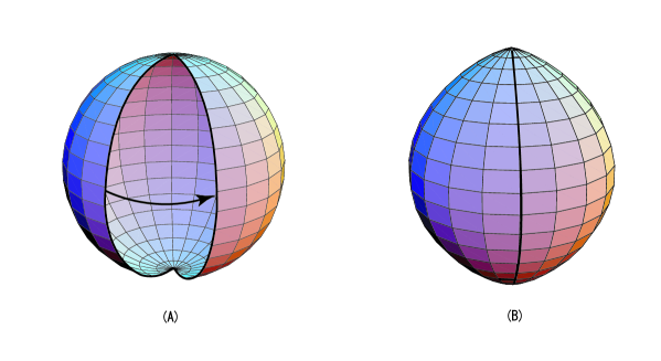
Figure 2: (A) The deficit angle $2\pi(1-\sqrt{1-2m})\sim 2\pi m$ is shown. (B) The conical singularity in the closed surface is formed gluing edges of the deficit angle shown in (A).

Next, we attempt to determine the scale factor of the universe including the quantum effect using the dBB equation. The explicit form of the dBB equation for the scale factor given by Eq. (36) becomes

$$\dot{a}(t)=\sqrt{\lambda a(t)^{2}-K}\,\frac{2}{\pi Z\mid H_{\nu}^{(2)}(Z)\mid^{2}}\ ,$$ (40)

where the variables in the case of de Sitter universe are

$$Z = \int dr(\bar{\Lambda}\sqrt{\chi-F_{j}}-\sqrt{1-2m}\,a(t)\ln\mid\frac{\sqrt{\chi}+\sqrt{\chi-F_{j}}}{\sqrt{\mid F_{j}\mid}}\mid)\ ,$$

$$\bar{\Lambda} = {a(t)}/{\sqrt{1-Kr^{2}}}\ ,$$

$$\chi = (1-2m)(1-Kr^{2})\ ,$$

$$F_{j} = (1-2m)(1-\lambda a(t)^{2}r^{2})\ .$$

The quantum effect is included in the factor ${2}/({\pi Z\mid H^{(2)}_{\nu}(Z)\mid^{2}})$ in Eq. (40). For the flat de Sitter universe ($K=0$), no quantum effect is obtained, because $Z$ becomes infinite as a result of due to the spatial integration over the infinite range of the variable $r$. For the closed de Sitter universe ($K=1$), a finite quantum effect is obtained only in the special case $\nu=1/3$. The result of the numerical analysis of the dBB equation in this special case with the scale factor $a(t)$ for the closed de Sitter universe given by Eq. (40) are presented in Fig. 3. These results confirm that the quantum scale factors with and without the conical singularity approache the classical scale factor asymptotically as

$$a(t)\mid_{m\neq 0}\approx a(t)\mid_{m=0}\approx a(t)_{cl}\approx\exp{(\sqrt{\lambda}t)}\ \ {\rm{as}}\ t\rightarrow{\rm large}\ .$$ (41)

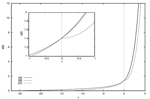
Figure 3: (A) The quantum scale factor in the case without a conical singularity ($m=0$). (B) The quantum scale factor in the case with a conical singularity ($m\neq 0$). (C) The classical scale factor in the case with a conical singularity ($m\neq 0$). The classically allowed region is $t>0$ and the classically forbidden region is $t<0$. Each scale factor is normalized such that $a(t=0)=\sqrt{1/\lambda}$. The parameters are chosen as $\lambda=1/2\ ,\ m=1/5$.

The quantum effects appear remarkably near the beginning of the universe as the derivation from the classical solution. We can show the relations for differentiation of the scale factor $a(t)$ with respect to $t$ at the beginning of the classical universe $a(t)=1/\sqrt{\lambda}$

$$\dot{a}(t)\mid_{m\neq 0} = (1-2m)^{-1/6}\frac{3^{4/3}\lambda^{1/6}}{4\pi}\Gamma{(2/3)}=(1-2m)^{-1/6}\dot{a}(t)\mid_{m=0}\ \$$ (42)

$$> \dot{a}(t)\mid_{m=0}\ \$$

$$> \dot{a}(t)\mid_{cl}=0.$$

These relations together with the asymptotic relations for the scale factor given by Eq. (41) imply the following hierarchy relations for $\dot{a}(t)$ at a given of $a(t)$

$$\dot{a}(t)\mid_{m\neq 0}\ >\ \dot{a}(t)\mid_{m=0}\ >\ \dot{a}(t)_{cl}\ \ .$$ (43)

The validity of these relations can be seen directly from Fig. 3. From these result given by Eq. (43), we confirm that the quantum effect becomes large as the mass parameter becomes large.

4 Summary

We have studied the (2+1)-dimensional Einstein theory of gravity with a cosmological constant within the framework of the ADM canonical formalism employing the de Broglie-Bohm interpretation. We examined the conical singularity in the de Sitter universe as a topological effect on the geometry. The classical limit is realized for this theory in the large universe limit, $a(t)\rightarrow\infty$. No quantum effect is obtained for the flat de Sitter universe solution, because in this case the volume of the universe and the value of $Z$ both become infinite. A finite quantum effect is obtained for the closed de Sitter universe solution with the parameter choice $\nu=1/3$ . The quantum effect on the scale factor becomes large as the mass of the point particle becomes large, as can be seen from Eq.(43) and Fig. 3. In the closed de Sitter universe solution, a conical singularity occurs due to the presence of the mass $m$, and in this case the volume of the universe is small. We can summarize our results as follows: The size of the quantum effects increases as the size of the universe decreases. This relation is consistent with our general experience: quantum effects are larger for smaller objects.

As future problems, we are interested in determining the quantum effect for the anti-de Sitter universe using the dBB interpretation. We are also interested in the total gravitational energy of a massive point particle in a closed universe. We plan to study a torus as an example of other topologies in the (2+1)-dimensional gravity theory [21].

Finally, it is worthwhile to note the difference between the dBB interpretation and the interpretation by the WKB approach. Though the concepts of the two interpretations are very different, the basic equations are very similar. In the semi-classical region, both solutions obtaining by the dBB interpretation and by the WKB approach become almost the same, and in addition the dBB interpretation requires a smooth extension into the classically forbidden region. For these reasons, we assert that the dBB interpretation is more natural than the WKB approach.

Acknowledgements

We would like to thank Dr. T. Takahashi for useful discussions and numerical calculations.

References

- [1] J. Polchinski, String Theory I, II (Cambridge University Press, 1998).
- [2] See for example, C.M. Hull and P.K. Townsent, Nucl. Phys. B 438 (1995) 109; E. Witten, Nucl. Phys. B 443 (1995) 85; J.H. Shwarz, Phys. Lett. B 367 (1996) 97.
- [3] See for example, J. Maldacena, Adv. Theor. Math. Phys. 2 (1998) 231; E. Witten, Adva. Theor. Math. Phys. 2 (1998) 253.
- [4] See for example, A. Strominger and C. Vafa, Phys. Lett. B 379 (1996) 99.
- [5] A. Achúcarro and P.K. Townsend, Phys. Lett. B 180 (1986) 89.
- [6] E. Witten, Nucl. Phys. B 311 (1988) 46.
- [7] J.D. Brown and M. Henneaux, Comm. Math. Phys. 104 (1986) 207.
- [8] S. Carlip, Phys. Rev. D 51 (1995) 632.
- [9] K. Ezawa, Int. J. Mod. Phys. A 19 (1995) 4139.
- [10] M. Bañados, Phys. Rev. D 52 (1996) 5816.
- [11] Y. Yoshida and T. Kubota, Phys. Rev. D 60 (1999) 044013.
- [12] S. Deser, R. Jackiw and G.t’ Hooft, Ann. Phys. 152 (1984) 220.
- [13] P.A.M. Dirac, The theory of gravitation in Hamiltonian form, Proc. Roy. Soc. A 246 , (1958) 333.
- [14] R. Arnowitt, S. Deser, and C.W. Misner, in Gravitation: An introduction to Current Research, edited by L. Witten (Wiley, New York, 1962).
- [15] M. Bañados, C. Teitelboim and J. Zanelli, Phys. Lett. 69 (1992) 1849.
- [16] See for example, D. Bohm, Phys. Rev 85 (1952) 166, 180; J.S. Bell, Speakable and Unspeakable in Quantum Mechanics, Cambridge University Press, Cambridge, England (1987); P.R.Holland, The Quantum Theory of Motion, Cambridge University Press, Cambridge, England (1993).
- [17] S.P.de Alwis and D.A. MacIntire, Phys. Rev. D 50 (1987) 3626; M. Kenmoku, K. Otsuki, K. Shigemoto and K. Uehara, Class. Quantum Grav. 13 (1996) 1751; M. Kenmoku, H. Kubotani, E. Takasugi and Y. Yamazaki, Phys. Rev. D 57 (1998) 4952.
- [18] K.V. Kuchař, Phys. Rev. D 50 (1994) 3961.
- [19] M. Kenmoku, H. Kubotani, E. Takasugi and Y. Yamazaki, Prog. Theor. Phys. 105 (2001) 897.
- [20] A. Vilenkin, Phys. Rev. D 37 (1988) 888.
- [21] A. Hosoya and K. Nakao, Prog. Theor. Phys. 84 (1990) 739.