Four-dimensional anti–de Sitter toroidal black holes from a three-dimensional perspective: full complexity

Abstract

The dimensional reduction of black hole solutions in four-dimensional (4D) general relativity is performed and new 3D black hole solutions are obtained. Considering a 4D spacetime with one spacelike Killing vector, it is possible to split the Einstein-Hilbert-Maxwell action with a cosmological term in terms of 3D quantities. Definitions of quasilocal mass and charges in 3D spacetimes are reviewed. The analysis is then particularized to the toroidal charged rotating anti-de Sitter black hole. The reinterpretation of the fields and charges in terms of a three-dimensional point of view is given in each case, and the causal structure analyzed.

PACS numbers: 04.40.Nr, 04.70.Bw, 04.20.Jb.

I Introduction

The work on three-dimensional (3D) gravity theories has seen a great impulse after the discovery that 3D general relativity possesses a black hole solution, the Bañhados-Teitelboim-Zanelli (BTZ) black hole btz ; bhtz . Before the appearance of this black hole solution there were, however, important works in 3D general relativity which studied the properties of point particles in 3D geometries deser1 ; deser2 as well as solutions with matter giddings , and showed that it provides a testbed for 4D and higher-D theories achucarro ; witten . In addition there were works in 3D string theory with its associated black strings horowitz1 ; horowitz2 . However, because of the lack of black holes there was no possibility of discussing important issues such as the entropy of the gravitational field, its degrees of freedom, and Hawking evaporation. The work by Bañados, Teitelboim, Zanelli, and Henneaux btz ; bhtz brought then 3D general relativity into the level of complexity of 4D general relativity. This black hole is a solution of the Einstein-Hilbert action including a negative cosmological constant term $\Lambda$. One can also show that the BTZ black hole can be constructed by identifying certain points of the 3D anti–de Sitter (AdS) spacetime bhtz . Since the AdS spacetime is a simple manifold one can study many properties of the BTZ black hole through known results in AdS spaces, upon making further appropriate global identifications (see carlip for a review).

After the BTZ solution a whole set of new solutions in 3D followed from a number of different dilaton-gauge vector theories coupled to gravity. For instance, upon reducing 4D Einstein-Maxwell theory with $\Lambda$ and with one spatial Killing vector it was shown in lemos1 ; lz1 that it gives rise to a 3D Brans-Dicke-Maxwell theory with its own black hole, which when reinterpreted back in 4D is a black hole with a toroidal horizon. One can then naturally extend the whole set to Brans-Dicke theories sa ; dias1 . Other solutions with different couplings have also been found chan ; martinez (see dias1 for a more complete list).

One important ingredient in these solutions is the presence of a negative cosmological constant, $\Lambda<0$. The interest in these solutions appeared after it was shown that gauged supergravity requires for its ground state a $\Lambda<0$ term, such that spacetime is AdS or asymptotically AdS. Many of these black holes, such as the BTZ black hole, only exist in theories with a negative $\Lambda$ ida , which in turn motivated their further study. A renewal of interest in these solutions came after the AdS-conformal field theory (AdS-CFT) conjecture maldacena . This conjecture states the equivalence between string theory on an AdS background and a corresponding CFT defined on the boundary of AdS spacetime, i.e., between AdS_n and a CFT_n-1. The $n=3$ case (i.e., 3D), mainly through the BTZ black hole, plays an important role in the verification of the conjecture, since many higher-D extreme black holes of string theory have a near-horizon geometry containing the BTZ black hole. Then the conjecture says that if one has, e.g., a 10-dimensional type IIB supergravity, compactified into a ${\rm BTZ}\times S^{3}\times T^{4}$ spacetime, the BTZ in the bulk corresponds to a thermal state in the boundary CFT maldacenastrominger . It is also possible to embed the 4D toroidal black holes lemos1 ; lz1 in a higher-D string theory such that they can be interpreted as the near horizon structures of an $M2$ brane rotating in extra dimensions duff .

Now, in order to find solutions in a given dimension, $n$ say, one usually starts from the action of gravity theory with the generic dilaton and gauge vector couplings in that dimension, derives the corresponding equations of motion, tries an ansatz for the solution and then finally from the differential equations finds the black hole solutions compatible with the ansatz. This is the case for the Schwarzschild solution for instance, and for many of the 3D solutions quoted above. Another way of finding solutions arises if the theory possesses dualities, i.e., symmetries that convert one solution into another in a nontrivial way horowitzreview92 . Yet another way, which can be seen as a special case of duality, is through dimensional reduction, where one can reduce a theory by several dimensions. The simplest case is to reduce by one dimension, i.e., one starts with a ($n+1$)D Lagrangian theory and through a suitable procedure reduces it along a symmetry direction into a new $n$D Lagrangian theory. There are a number of inequivalent procedures to perform a dimensional reduction, two of those are the dimensional reduction through a Kaluza-Klein ansatz (or classical Kaluza-Klein reduction) duff2 , and the Lagrangian dimensional reduction cremmer . When one is reducing through one symmetric compact direction (a circle), which will be the cases studied here, both procedures are equivalent duff2 ; breiten . In the reduction process scalars and gauge vector fields appear naturally. The symmetry direction of the solution in the ($n+1$)D theory defines a Killing vector and a Killing direction, which in general can be compact or non-compact. In turn, in the non-compact case the reduction process can be important to the original theory in ($n+1$)D. For example, for a black hole solution in the lower $n$D theory one can give precise definitions of charges (mass, angular momentum, electromagnetic, dilaton and axion charges), which in the ($n+1$)D theory are then converted into charges per unit length of the corresponding black string lemos1 ; abicaks . In the past two decades, due to the extra dimensions required by supergravity and string theories, the techniques of compactification and dimensional reduction have became powerful tools to build and analyze black hole solutions in lower dimensions (see, e.g., horowitzreview92 ; cremmer ; duff2 ; breiten ; abicaks ; KSS ).

In this paper we follow the classical Kaluza-Klein procedure, here equivalent to the Lagrangian dimensional reduction procedure, to find new solutions in 3D from solutions in 4D. An extensive study of 4D solutions of gravity coupled to sigma model theories and their corresponding Kaluza-Klein 3D counterparts has been performed breiten , in which, in the last section of the paper on “Open Problems” the authors state that the inclusion of a cosmological constant is important. It is our aim to apply the dimensional reduction technique to construct 3D black holes from the 4D toroidal AdS black holes lemos1 ; lz1 . Sect. II is dedicated to a review of the dimensional reduction method particularized to the case of reduction from 4D to 3D. The definition of the charges for all fields, new and old, appearing in 3D is also given. Then, in Sect. III, dimensional reduction, through the Killing azimuthal direction $\partial/\partial\varphi$, of rotating charged black holes with toroidal topology is considered. The produced 3D black holes display an isotropic horizon (i.e., circularly symmetric), and the new charges are neatly found. In Sect. IV we conclude.

II Dimensional Reduction

II.1 The action, the Lagrangian and the fields

In this subsection we discuss the connection between the Einstein-Maxwell-AdS equations in a four-dimensional (4D) spacetime with a Killing vector and the equations in the corresponding 3D spacetime. We assume that the 4D manifold ${\cal M}_{4}$ can be decomposed as ${\cal M}_{4}={\cal M}\times{\cal S}^{1}$ or ${\cal M}_{4}={\cal M}\times R$, with $\cal M$, ${\cal S}^{1}$, and $R$ being the 3D manifold, the circle, and the real line, respectively.

The action $\hat{S}$ in 4D spacetimes is assumed to be the usual Einstein-Hilbert-Maxwell action with cosmological term $\hat{\Lambda}$ and electromagnetic field $\hat{\bf F}={\rm d}\hat{\bf A}$ (where $\hat{\bf A}$ is the gauge field), given by (we use geometric units where $G=1$, $c=1$),

$$\hat{S}=\int d^{4}x\,{\hat{\cal L}}=\frac{1}{16\pi}\int{d^{4}x\sqrt{-\hat{g}}\left(\hat{R}-2\hat{\Lambda}-\hat{F}^{2}\right)}\,,$$ (1)

where ${\hat{\cal L}}$ is the Lagrangian density, or Lagrangian. The convention adopted here is that quantities wearing hats are defined in 4D and quantities without hats belong to 3D manifolds. We now proceed with the reduction of the action (1) to 3D. In order to do that consider then a 4D spacetime metric admitting one spacelike Killing vector, $\displaystyle{\partial_{\varphi}}$, where $\varphi$ can be a compact or a non-compact direction. In such a case the 4D metric may be decomposed into the form

$$d{\hat{s}}^{2}=e^{2\beta_{0}\phi}ds^{2}+e^{2\beta_{1}\phi}\left(d\varphi+{\cal A}_{i}dx^{i}\right)^{2}\,,$$ (2)

where $ds^{2}$ is the 3D metric, $\phi$, ${\cal A}_{i}$ ($i=0,1,2$) and all the other metric coefficients are functions independent of $\varphi$, and $\beta_{0}$, $\beta_{1}$ are numbers. To dimensionally reduce the electromagnetic gauge field we do

$$\hat{\bf A}={\bf A}+A_{\varphi}{\rm\bf d}\varphi\,,$$ (3)

where for compact $\varphi$ the gauge group is $U(1)$ and for non-compact $\varphi$ it is $R$. In the last equation $\bf A$ is a $1$-form while $A_{\varphi}$ is a $0$-form. In terms of a coordinate basis in the 3D manifold this means that $\bf A$ and $A_{\varphi}$ correspond to a vector field $A_{i}$ and to a scalar field $A_{\varphi}=\Psi$, say, respectively. From these fields we can define the 3D Maxwell field

$$\bf F={\rm{\bf d}}\bf A\,.$$ (4)

It is convenient to define a new 2-form $\bf E$ as

$${\bf E}\equiv{\bf F}-{\bf d}\Psi\wedge{\cal A}\,,$$ (5)

where ${\cal A}$ is the Kaluza-Klein gauge field 1-form appearing in the 4D metric (2).

The Kaluza-Klein dimensional reduction procedure then gives

$$S = \frac{L_{3}}{16\pi}\int{d^{3}x\sqrt{-g}e^{(\beta_{0}+\beta_{1})\phi}\left[R-2\Lambda e^{2\beta_{0}\phi}+2\beta_{0}(\beta_{0}+2\beta_{1})\left(\nabla\phi\right)^{2}\right.}$$ (6)

$$\left.-{}e^{-2\beta_{0}\phi}E^{2}-{1\over 4}e^{2(\beta_{1}-\beta_{0})\phi}{\cal F}^{2}-{2}e^{-2\beta_{1}\phi}({\bf\nabla}\Psi)^{2}\right]\,,$$

where we have defined

$${\cal F}={\bf d}{\cal A}\,.$$ (7)

The 3D cosmological constant is defined as $\Lambda=\hat{\Lambda}$. $L_{3}$ is the result of integration along the $\varphi$ direction. Assuming the spacetime is compact along the generic spacelike dimension parametrized by $\varphi$, then $L_{3}$ is given by the range of $\varphi$ and will be dimensionless, while for noncompact $\varphi$, $L_{3}$ carries physical units of length. From the 3D point of view, $L_{3}$ can be thought of as the size of the extra dimension. The explicit form of $E^{2}$ in terms of the 3D fundamental fields $F_{ij}$, ${\cal A}_{i}$ and $\Psi$ is

$$E^{2}\equiv E_{ij}E^{ij}=F^{2}+4F^{ij}{\cal A}_{i}\,\nabla_{j}\Psi+2\left[({\bf\nabla}\Psi)^{2}{\cal A}^{2}-({\cal A}^{i}\,{\nabla_{i}}\Psi)^{2}\right]\,.$$ (8)

The reduced action shows two different gauge fields. The first one, $A_{i}$, is the 3D counterpart of the 4D electromagnetic gauge field. The second, ${\cal A}_{i}$, is the Kaluza-Klein gauge field. There are also two scalar fields. The dilaton $\phi$, and another scalar field $\Psi$, which is the projection of the 1-form gauge field $\hat{\bf A}$ onto the Killing direction $\varphi$. The scalar field $\Psi$ couples to the metric differently from a true scalar field. This can be seen, for instance, by comparing the last term in the action (6) to the kinetic term for the dilaton field $(\nabla\phi)^{2}$.

The equations of motion which follow from the action (6) for the graviton $\bf g$, the gauge fields $\bf A$ and $\cal A$, the dilaton $\phi$, and the scalar $\Psi$ are, respectively:

$$G_{ij}=-\Lambda e^{2\beta_{0}\phi}g_{ij}+(\beta_{0}+\beta_{1})\left[\nabla_{i}\nabla_{j}\phi-(\beta_{0}+\beta_{1})\nabla_{i}\phi\nabla_{j}\phi-g_{ij}\nabla^{2}\phi\right]$$

$$\hskip 34.14322pt+\beta_{1}^{2}\left[2\nabla_{i}\phi\nabla_{j}\phi-g_{ij}\left(\nabla\phi\right)^{2}\right]-{2}e^{-2\beta_{0}\phi}\left[E_{ik}E^{k}_{j}+{1\over 4}g_{ij}E^{2}\right]$$

$$\hskip 34.14322pt-{1\over 2}e^{2(\beta_{1}-\beta_{0})\phi}\left[{\cal F}_{ik}{\cal F}^{k}_{j}+{1\over 4}g_{ij}{\cal F}^{2}\right]+{2}e^{-2\beta_{1}\phi}\left[\nabla_{i}\Psi\nabla_{j}\Psi-{1\over 2}g_{ij}(\nabla\Psi)^{2}\right]\,,$$ (9)

$$\nabla_{j}\left[e^{(\beta_{1}-\beta_{0})\phi}\left(F^{ij}-{\cal A}^{i}\nabla^{j}\Psi+{\cal A}^{j}\,\nabla^{i}\Psi\right)\right]=0\,,$$ (10)

$$\nabla_{j}\left[e^{(3\beta_{1}-\beta_{0})\phi}{\cal F}^{ij}\right]=4e^{(\beta_{1}-\beta_{0})\phi}\left[-F^{ij}\nabla_{j}\Psi+{\cal A}^{i}\left(\nabla\Psi\right)^{2}-\left(A^{j}\nabla_{j}\Psi\right)\nabla^{i}\Psi\right]\,,$$ (11)

$$\nabla_{i}\left[\beta_{1}^{2}e^{(\beta_{0}+\beta_{1})\phi}\nabla^{i}\phi\right]=-\Lambda\,\beta_{1}e^{(\beta_{1}+3\beta_{0})\phi}+{1\over 4}\beta_{1}{e^{(3\beta_{1}-\beta_{0})\phi}}{\cal F}^{2}$$

$$\hskip 36.98866pt+{1\over 2}\beta_{1}e^{(\beta_{1}-\beta_{0})\phi}E^{2}-\beta_{1}{e^{(\beta_{0}-\beta_{1})\phi}}\left(\nabla\Psi\right)^{2}\,,$$ (12)

$$\nabla_{i}\left[e^{(\beta_{0}-\beta_{1})\phi}\nabla^{i}\Psi+e^{(\beta_{1}-\beta_{0})\phi}\left(F^{ij}{\cal A}_{j}+{\cal A}^{2}\nabla^{i}\Psi-{\cal A}^{i}\,{\cal A}^{j}\nabla_{j}\Psi\right)\right]=0\,,$$ (13)

where $G_{ij}$ is the Einstein tensor.

Now, we are free to choose $\beta_{0}$ and $\beta_{1}$, i.e., we are free to choose the frame in which to work, with the different frames being related by conformal transformations. There are three frames that stand out:

(i) the good frame, i.e., the one that preserves most of the structure of the 4D spacetimes, is given by $\beta_{0}=0$ and $\beta_{1}$ free, which we can normalize to $\beta_{1}=-2$, yielding the following action $S_{\rm g}$ (for these three particular cases, we do not display the equations of motion, only the action since it is much more condensed)

$$S_{\rm g} = \frac{L_{3}}{16\pi}\int{d^{3}x\sqrt{-g}e^{-2\phi}\left[R-2\Lambda-E^{2}-{1\over 4}e^{-4\phi}{\cal F}^{2}-{2}e^{4\phi}({\bf\nabla}\Psi)^{2}\right]}\,;$$ (14)

(ii) the Einstein frame, the one that preserves the Einstein form of the action, is given by choosing $\beta_{0}+\beta_{1}=0$, and $\beta_{0}=1/2$, so that the kinetic term of the dilaton is $2\beta_{0}(\beta_{0}+2\beta_{1})=-1/2$ (see e.g. KSS for dimensional reduction in the Einstein frame), yielding the action $S_{\rm E}$

$$S_{\rm E} = \frac{L_{3}}{16\pi}\int{d^{3}x\sqrt{-g}\left[R-2\Lambda e^{\phi}-{1\over 2}\left(\nabla\phi\right)^{2}-e^{-\phi}E^{2}-{1\over 4}e^{-2\phi}{\cal F}^{2}-{2}e^{\phi}({\bf\nabla}\Psi)^{2}\right]}\,;$$ (15)

(iii) the string frame, where one chooses $\beta_{0}+\beta_{1}=-2$ and $\beta_{0}=-2\pm\sqrt{2}$, fixing the kinetic term of the dilaton to $2\beta_{0}(\beta_{0}+2\beta_{1})=4$, yielding the following action $S_{\rm s}$

$$S_{\rm s} = \frac{L_{3}}{16\pi}\int{d^{3}x\sqrt{-g}e^{-2\phi}\left[R-2\Lambda e^{-2(2\mp\sqrt{2})\phi}+4\left(\nabla\phi\right)^{2}\right.}$$ (16)

$$\left.-e^{2(2\mp\sqrt{2})\phi}E^{2}-{1\over 4}e^{4(1\mp\sqrt{2})\phi}{\cal F}^{2}-{2}e^{\pm 2\sqrt{2}\phi}({\bf\nabla}\Psi)^{2}\right]\,.$$

It is well known that the different frames, related by conformal transformations, are physically inequivalent, e.g., one frame can give spacetime singularities where the other does not (see, e.g., chan-mann ; marolf ). We will work mainly with the good frame, and we will comment later on the other frames.

As it will be seen later on, the 3D solutions are obtained from the 4D metric and the other 4D fields by direct inspection of the metric and correct truncation of extra fields. This task is more easily accomplished by working in the good frame. Once we have the 3D metric in the good frame ($\beta_{0}=0$), the metric in any other frame can be obtained by the appropriate conformal transformation. In order to build such a transformation, let us define $ds^{2}_{\rm g}$ and $ds^{2}_{\rm o}$ as the given metric written in the good and other frames, respectively. In the good frame, the parameters $\beta_{0}$ and $\beta_{1}$ assume respectively the values $(\beta_{0})_{\rm g}$ and $(\beta_{1})_{\rm g}$ [as we have mentioned, we chose $(\beta_{0})_{\rm g}=0$ and $(\beta_{1})_{\rm g}=-2$]. Let us also denote the values assumed by the parameters $\beta_{0}$ and $\beta_{1}$ in the other frame, respectively, by $(\beta_{0})_{\rm o}$ and $(\beta_{1})_{\rm o}$. The two frames are then related by

$$ds^{2}_{\rm o}=\left(e^{-2\beta_{1}\phi}\right)_{\!{\rm g}}^{\left(\beta_{0}/\beta_{1}\right)_{\!\rm o}}ds^{2}_{\rm g}\,,$$ (17)

where $\left(e^{2\beta_{1}\phi}\right)_{\rm g}$ is the dilaton field in the good frame. For instance, the relation between good and Einstein frames is $ds^{2}_{{}_{\rm E}}=\left(e^{2\beta_{1}\phi}\right)_{\!{\rm g}}ds^{2}_{\rm g}$.

II.2 The global charges

Now we study how to define mass, angular momentum and charges in the 3D spacetime by using the formalism of Brown and York by1 ; brown-mann ; creighton-mann modified to include a dilaton and other fields.

II.2.1 The conventions

We assume that the 3D spacetime $\cal M$ is topologically the product of a spacelike surface $D_{2}$ and a real line time interval $I$, ${\cal M}=D_{2}\times I$. $D_{2}$ has the topology of a disk. Its boundary $\partial D_{2}$ has the topology of a circle and is denoted by ${\cal S}_{1}$. The boundary of $\cal M$, $\partial\cal M$, consists of two spacelike surfaces $t=t_{1}$ and $t=t_{2}$, and a timelike surface ${\cal S}_{1}\times I$ joining them. Let $t^{i}$ be a timelike unit vector ($t_{i}t^{i}=-1$) normal to a spacelike surface $D_{2}$ (that foliates $\cal M$), and $n^{i}$ be the outward unit vector normal to the boundary $\partial\cal M$ ($n_{i}n^{i}=1$). Let us denote the spacetime metric on $\cal M$ by $g_{ij}$ ($i,j=0,1,2$). Hence $h_{ij}=g_{ij}+t_{i}t_{j}$ is the induced metric on $D_{2}$ and $\sigma_{ij}=g_{ij}+t_{i}t_{j}-n_{i}n_{j}$ is the induced metric on ${\cal S}_{1}$. $h_{ij}$ can be viewed also as a tensor $h_{mn}$ ($m,n=1,2$) on $D_{2}$, and $\sigma_{ij}$ can be viewed as a scalar (a tensor of rank zero) $\sigma_{ab}\equiv\sigma$ ($a,b=2$) on the one-dimensional boundary ${\cal S}_{1}$. Since ${\cal S}_{1}$ is a one-dimensional space, the induced metric $\sigma_{ab}$ has only one independent component. The induced metric on the spacetime boundary $\partial\cal M$ is $\gamma_{ij}=g_{ij}-n_{i}n_{j}=\sigma_{ij}-t_{i}t_{j}$. We also assume that the spacetime admits the two Killing vectors needed in order to define mass and angular momentum: a timelike Killing vector $\eta_{t}^{i}=({\partial}/{\partial t})^{i}$ and a spacelike (axial) Killing vector $\eta_{\theta}^{i}=(\partial_{\theta})^{i}$.

II.2.2 Mass

The next step is to adapt the Brown and York procedure to take into account the dilaton field creighton-mann . By doing this, we arrive at the following definition of mass $M$ on a 3D spacetime admitting a timelike Killing vector $\eta_{t}$

$$M_{3D}={L_{3}\over 8\pi}\int_{{\cal S}_{1}}e^{2(\beta_{0}+\beta_{1})\phi}\delta\left({k^{\phi}}\right)t_{i}\eta_{t}^{i}\,d{\cal S}\,,$$ (18)

where $t^{i}$ is the timelike future pointing normal to $D_{2}$, $d{\cal S}=\sqrt{\sigma}\,d\xi$ with $\xi$ being a coordinate on ${\cal S}_{1}$, and $\sigma$ being the determinant of the induced metric on ${\cal S}_{1}$ (since ${\cal S}_{1}$ is a one-dimensional space, the determinant $\sigma$ of the induced metric $\sigma_{ab}$ coincides with the metric itself). ${k^{\phi}}$ is the trace of the extrinsic curvature of ${\cal S}_{1}$ as embedded on $D_{2}$, modified by the presence of the dilaton. To define ${k^{\phi}}$ explicitly we consider the particular case when the two-metric on $D_{2}$ can be split as

$$ds_{D_{2}}^{2}=h_{mn}dx^{m}\,dx^{n}=f^{2}dr^{2}+R^{2}\left(d\xi+V\,dr\right)^{2}\,,$$ (19)

where $m,n=1,2$, $x^{1}=r$, $x^{2}=\xi$, and $\xi$ parametrizes ${\cal S}_{1}$. Functions $f$, $R$ and $V$ depend on all coordinates. $k^{\phi}$ may then be written as

$${k^{\phi}}=-{e^{-(\beta_{0}+\beta_{1})\phi}\over 2}{1\over f}\left({2\over R}{\partial R\over\partial r}+2\left(\beta_{o}+\beta_{1}\right){\partial\phi\over\partial r}-\nabla_{\xi}V\right)\,,$$ (20)

where $\nabla_{\xi}$ is the covariant derivative on ${\cal S}_{1}$. Recall that the energy surface density on ${\cal S}_{1}$, $\epsilon$, is given by

$$\epsilon=\frac{k^{\phi}}{8\pi}\,.$$ (21)

An explicit definition of $\epsilon$ is given for the particular case studied in Sect. III below. In Eq. (18), the symbol $\delta$ indicates the difference between the extrinsic curvature $k^{\phi}$ on the spacetime $\cal M$ obtained from the full action $S$, say, and the corresponding quantity $\left(k^{\phi}\right)_{\!o}$ obtained from a reference spacetime ${\cal M}_{o}$, solution of a reference action $S_{o}$. Namely, $\delta({k^{\phi}})={k^{\phi}}-({k^{\phi}})_{o}$. In this paper we are interested in black holes in asymptotically AdS spacetimes. Hence, the action $S$ refers to a specific black hole solution as, e.g., the toroidal rotating charged-AdS spacetime, and $S_{o}$ refers to the (asymptotic) AdS spacetime, when no black hole is present. The right hand side of Eq. (18) is the quasilocal mass as defined in Brown-York formalism and in general depends on the choice of the boundary ${\cal S}_{1}$. In our definition we assume that ${\cal S}_{1}$ represents the infinite boundary of the two-space $D_{2}$, and the integration over ${\cal S}_{1}$ then gives the global mass associated with the considered black hole solution.

II.2.3 Angular momentum

Similarly to the mass, the definition of angular momentum $J$ for a 3D spacetime admitting a spacelike Killing vector $\partial_{\theta}=\eta_{\theta}$ can also be modified to include the dilaton. The definition of the angular momentum is then

$$J_{3D}={L_{3}}\int_{{\cal S}_{1}}e^{2(\beta_{0}+\beta_{1})\phi}\delta\left({j^{\phi}}_{i}\right)\eta_{\theta}^{i}\,d{\cal S}\,,$$ (22)

where ${j^{\phi}}_{i}$ is the momentum surface density on ${\cal S}_{1}$, modified by the presence of the dilaton. We also have $\delta({j^{\phi}}_{i})\equiv(j^{\phi}_{i})-(j^{\phi}_{i})_{o}$, where $(j^{\phi}_{i})_{o}$ is the angular-momentum density at the boundary ${\cal S}_{1}$ of the background (or reference) spacetime, and ${j^{\phi}}_{i}$ is the full angular momentum density of the considered spacetime. We do not give here an explicit definition for ${j^{\phi}}_{i}$, since it will not be needed in the applications considered in the present work.

Since we are interested in the global conserved quantities of black holes, in Eq. (22), as in Eq. (18) and in the charges defined below, the integral over the boundary of $D_{2}$, ${\cal S}_{1}$, is in fact taken at the infinity of $D_{2}$, ${\cal S}_{1}\longrightarrow\infty$. In such a limit, the mass, angular momentum, and charges defined according to the Brown and York formalism coincide with the ADM mass, angular momentum and charges.

Now we turn our attention to the definition of other charges in 3D spacetimes.

II.2.4 Electric and magnetic charges

(a)  Electric charges of the gauge fields $A_{i}$ and ${\cal A}_{i}$. The two gauge fields, $A_{i}$ and ${\cal A}_{i}$, have different electric charges $Q_{e}$ and ${\cal Q}_{e}$, respectively, and both are coupled to the scalar field $\Psi$, besides being coupled to each other. Moreover, $A_{i}$ couples to $\Psi$ through kinetic terms, whereas ${\cal A}_{i}$ couples through potential terms. Both gauge charges can be obtained by the Gauss law, adapted to non-asymptotically flat stationary spacetimes and to the presence of the dilaton by1 ; creighton-mann (see also lemos1 ; lz1 )

$${Q_{e}}={L_{3}\over 4\pi}\int_{{\cal S}_{1}}{\delta E_{i}n^{i}}d{\cal S}\,,$$ (23)

$${\cal Q}_{e}={L_{3}\over 4\pi}\int_{{\cal S}_{1}}{\delta{\cal E}_{i}n^{i}}d{\cal S}\,,$$ (24)

where $E_{i}\equiv e^{(\beta_{1}-\beta_{0})\phi}F_{ij}t^{j}$, ${\cal E}_{i}\equiv e^{(3\beta_{1}-\beta_{0})\phi}{\cal F}_{ij}t^{j}/4$, $n^{i}$ is the unit normal to the spacelike one-dimensional surface ${\cal S}_{1}$, a circle, and $t^{i}$ is the timelike normal to the two-space ($D_{2}$), a disk. Here also ${\cal S}_{1}$ is the infinite border of $D_{2}$. As in the definition of mass and angular momentum, the symbol $\delta$ indicates the difference between the quantity in question in the considered spacetime and the same quantity in a reference spacetime. Namely, $\delta E_{i}=E_{i}-(E_{i})_{o}$ and $\delta{\cal E}_{i}={\cal E}_{i}-({\cal E}_{i})_{o}$. Quantities $E^{i}$ and ${\cal E}^{i}$ can be interpreted as electric fields in the two-space orthogonal to $t^{i}$. $(E_{i})_{o}$ and $({\cal E}_{i})_{o}$ are the electric field strengths for the background (or reference) spacetime, when no localized objects are present. The integrals in Eqs. (23) and (24) are taken at spatial infinity. Hence, in order to obtain a well defined charge in spacetimes asymptotically AdS, we must subtract the background value from the corresponding global charge, and this procedure has to be applied to every charge of the model.

It is worth mentioning that both of the electric charges are built from conserved currents $J_{e}^{i}\equiv\nabla_{j}\left(e^{(\beta_{1}-\beta_{0})\phi}F^{ij}\right)$ and ${\cal J}_{e}^{i}\equiv\nabla_{j}\left(e^{(3\beta_{1}-\beta_{0})\phi}{\cal F}^{ij}/4\right)$, respectively, for which follow immediately $\nabla_{i}J_{e}^{i}=0$ and $\nabla_{i}{\cal J}_{e}^{i}=0$ (see also the item (c), in this section, below). These two identities guarantee the existence of the two conserved electric charges as defined above.

(b) Magnetic charges of the gauge fields $A_{i}$ and ${\cal A}_{i}$. The magnetic charges in 3D spacetimes have world histories with dimension zero. They are events in the spacetime (instantons) teitel ; pisarski since the dual field strength in 3D is not a 2-form, but a 1-form, i.e., ${}^{*}\!{\bf F}$ yields the 1-form $B_{i}=\epsilon_{ijk}F^{jk}/2$. Thus, integration over the boundary of $D_{2}$ at infinity cannot be performed in the same way as one does for the electric charge. However, we can think of the divergence $\nabla_{i}B^{i}$ as the magnetic charge density and an integration over the spacetime 3D world volume $\Sigma$ yields the magnetic charges (or magnetic instantons). For stationary spacetimes, the divergence $\nabla_{i}B^{i}$ defines an invariant charge density $\rho_{m}$ on the two-space $D_{2}$, and the volume integration over the whole $D_{2}$ yields the magnetic charge. Using Gauss theorem, the volume integral over $D_{2}$ is changed into a surface integral over the infinite boundary of $D_{2}$, i.e., over the ${\cal S}_{1}$ circle mentioned above. We can then define the magnetic charges in 3D by

$${Q_{m}}={L_{3}\over 4\pi}\int_{{\cal S}_{1}}{\delta B_{i}n^{i}}d{\cal S}\,,$$ (25)

$${\cal Q}_{m}={L_{3}\over 4\pi}\int_{{\cal S}_{1}}{\delta{\cal B}_{i}n^{i}}d{\cal S}\,,$$ (26)

where $B_{i}=e^{(\beta_{1}-\beta_{0})\phi}\,\epsilon_{ijk}F^{jk}/2$, ${\cal B}_{i}=e^{(3\beta_{1}-\beta_{0})\phi}\,\epsilon_{ijk}{\cal F}^{jk}/8$, and the integration is taken over a ${\cal S}_{1}$ surface, at the spatial infinity of $D_{2}$ (see above). These definitions apply at least for stationary spacetimes and do not include the “vortex magnetic charge” as defined by some authors, where the static magnetic field can be interpreted as being produced by a stationary electric current (vortex) (see Hirschwelch ; dias2 ). They are certainly useful in the case of instanton monopoles as defined in teitel ; pisarski ; helayel . Such definitions use the fact that, in 3D, the monopole generates a tangent electric field which can be used to determine the magnitude of the charge helayel (see Sect. III). Let us emphasize that the surface integrals in Eqs. (25) and (26) were obtained, using Gauss theorem, from a volume integration over the whole space $D_{2}$. Therefore, the magnetic charges defined in such a way are meaningful only if the surface integration is taken over the infinite boundary of $D_{2}$. For another discussion on the difficulties to define quasilocal gauge charges associated with 4D dyonic black holes see Ref. booth-mann .

(c) Deformations of the electromagnetic harges. An investigation on the field equations shows that the electromagnetic charges defined above may have additional contributions from the interaction terms with other fields. This is particularly true when $\Psi$ is nonzero, and the interaction terms between the gauge field ${\cal A}_{i}$ and the scalar $\Psi$ give rise to source terms in the field equations, in such a way that the conserved currents acquire extra terms that depend on $\Psi$ and on ${{\cal A}}$. To be more explicit, let us show what happens, for instance, regarding the electric charge $Q_{e}$. The full conserved current corresponding to the ${\bf F}$ field is

$$J^{j}=\nabla_{i}\left[e^{(\beta_{1}-\beta_{0})\phi}\left(F^{ij}+F_{\rm extra}^{ij}\right)\right]\,,$$ (27)

where $F_{\rm extra}^{ij}\equiv{\cal A}^{j}\nabla^{i}\Psi-{\cal A}^{i}\,\nabla^{j}\Psi$. Therefore, one should add a second term to Eq. (23) to give $\displaystyle{\int_{{\cal S}_{1}}{\delta\left(E_{i}+E^{\rm extra}_{i}\right)n^{i}}d{\cal S}}$, where $E^{\rm extra}_{i}=\displaystyle{e^{(\beta_{1}-\beta_{0})\phi}F^{\rm extra}_{ij}t^{j}}$. There are analogous correction terms related to the other electric charge, ${\cal Q}_{e}$, and also to the magnetic charges $Q_{m}$ and ${\cal Q}_{m}$. However, we find that for the black hole solutions we are going to analyze in this paper the above mentioned corrections to the conserved charges are zero. The extra terms, in fact, contribute to the quasilocal charges, when the boundary of integration ${\cal S}_{1}$ is not at infinity, but vanish at the infinite boundary of $D_{2}$.

II.2.5 Dilatonic charges

In addition to their mass and electromagnetic gauge charges, stationary asymptotically AdS 3D black holes are also characterized by the dilaton charge. As a matter of fact, two dilaton charges can be defined. The charge $Q_{\phi}$ ghs and its dual ${\tilde{Q}}_{\phi}$ gibbonsperry are given by

$$Q_{\phi}={L_{3}\over 4\pi}\int_{{\cal S}_{1}}{\delta\left(e^{(\beta_{0}+\beta_{1})\phi}\nabla_{i}\phi\right)n^{i}}d{\cal S}\,,$$ (28)

$${\tilde{Q}}_{\phi}={L_{3}\over 4\pi}\int_{{\cal S}_{1}}{\epsilon_{ijk}\delta\left(e^{(\beta_{0}+\beta_{1})\phi}\nabla^{k}\phi\right)n^{i}t^{j}}d{\cal S}\,,$$ (29)

where the integrations are defined in the same way as before.

The dilaton charge (28) is defined in Ref. ghs in the Einstein frame where $\beta_{0}+\beta_{1}=0$, and for $\Lambda\neq 0$ it is not related to a conserved current. It represents the total flux of the vector field $V_{i}=\nabla_{i}\phi$ across the surface ${\cal S}_{1}$ at the boundary of the space $D_{2}$. The result for $Q_{\phi}$ is the same to all stationary observers at infinity of $D_{2}$, and can then be identified with the charge of the dilaton field. It is a conserved charge just in the case $\Lambda=0$. Although this surface integral does not come from a conserved current, and perhaps should not be called a charge, we maintain it here because sometimes it has a nonzero value and is not totally useless (see ghs ; kalloshetal ).

The dual dilaton charge (29), on the other hand, is a conserved charge, since it is obtained from the conserved current ${\tilde{J}}_{\phi}^{i}=\nabla_{j}\left(\epsilon^{ijk}e^{(\beta_{0}+\beta_{1})\phi}\nabla_{k}\phi\right)$, which is divergence free $\nabla_{i}{\tilde{J}}_{\phi}^{i}=0$.

II.2.6 Charges of the scalar field $\Psi$

Finally, due to the presence of the scalar field $\Psi$ in the action (6) two other charges can also be defined. From Eq. (13) it is possible to identify the quantity $J_{\Psi}^{i}=e^{(\beta_{0}-\beta_{1})\phi}\nabla^{i}\Psi+e^{(\beta_{1}-\beta_{0})\phi}\left(F^{ij}{\cal A}_{j}+{\cal A}^{2}\nabla^{i}\Psi-A^{i}A^{j}\nabla_{j}\Psi\right)$ as a conserved current, $\nabla_{i}J_{\Psi}^{i}=0$. The corresponding conserved charge (analog to the electric charge) is

$$Q_{\Psi}={L_{3}\over 4\pi}\int_{{\cal S}_{1}}\delta\left(J_{\Psi}^{i}\right)n_{i}\,d{\cal S},$$ (30)

where the integration and the symbol $\delta$ have the same meaning as above. Let us mention that, for the solutions we are going to analyze here, the interaction terms between $\Psi$ and the gauge fields ${\bf A}$ and $\cal A$ do not contribute to the total charge for $\Psi$, and this charge is identically zero.

It is also possible to define a second conserved charge of topological character (which is the analog of the magnetic charge), also a source of the scalar field $\Psi$. From the vector quantity $\nabla^{i}\Psi$ we may construct an anti-symmetric dual tensor as $H_{ij}=\epsilon_{ijk}\nabla^{k}\Psi$. Therefore, the vector density $\nabla_{i}H^{ij}$ is divergence free and can be interpreted as a conserved current. Thus there is an associated conserved charge defined by

$${\tilde{Q}}_{\Psi}={L_{3}\over 4\pi}\int_{{\cal S}_{1}}{\epsilon_{ijk}\delta\left(\nabla^{k}\Psi\right)\,t^{i}n^{j}}d{\cal S}\,,$$ (31)

where the integration is the same as defined above. When ${\cal A}\neq 0$, there are additional terms in the equation of motion for $\Psi$ not considered to arrive at Eq. (31), but they do not contribute to the conserved charge [see the comments just after Eq. (26)].

II.2.7 General comments

We now study explicitly the connection between the general 4D stationary asymptotically AdS spacetimes and the corresponding 3D metrics obtained through the dimensional reduction technique discussed in the present section. We will reduce through the angular coordinate $\varphi$. We study 4D toroidal black holes in AdS spacetime, charged and rotating. These have a straightforward dimensional reducing procedure; the theory obtained is a 3D Brans-Dicke theory, and the 3D results are clear cut and simple; most frames (including the Einstein frame) are good frames.

III 3D Charged Rotating Toroidal Black Holes

III.1 The 4D metric and parameters

Hereafter we consider a class of rotating black holes with toroidal topology. In a previous paper lz1 we reported a rotating electrically charged black hole with a toroidal horizon. Before going on to the dimensional reduction of such a black hole, it is worth noting that following the same procedure as in lz1 a dyonic version of the black hole can be found.

We start constructing the static dyonic toroidal black hole by choosing the coordinate system $({t},r,\theta,{\varphi})$ with $-\infty<{t}<+\infty$, $0\leq r<+\infty$, $0\leq\theta<2\pi$, $0\leq{\varphi}<1$ (the ranges of the angular coordinates are arbitrary, we have chosen these particular ones to yield convenient values for the mass and charges).

The solution is found by solving Einstein-Maxwell equations for such a static spacetime. We find

$$d\hat{s}^{2} = -\left(\alpha^{2}r^{2}-\frac{4m}{r}+\frac{4(q^{2}+g^{2})}{r^{2}}\right)d{{t}}^{2}+\frac{dr^{2}}{\alpha^{2}r^{2}-\frac{4m}{r}+\frac{4(q^{2}+g^{2})}{r^{2}}}$$ (32)

$$+r^{2}\left(d{{\varphi}}^{2}+d\theta^{2}\right)\,,$$

$${\bf\hat{A}} = -{2q\over r}\,{\rm\bf d}t-{2g}\,\theta{\rm\bf d}\varphi\,,$$ (33)

where $\alpha^{2}\equiv-\frac{1}{3}\Lambda$, and $m$, $q$ and $g$ are integration constants. It is easy to show, for instance using Gauss law, that $q$ and $g$ are respectively the electric and magnetic charges of the black hole, and $m$ is its mass. Depending on the relative values of $m$, $q$ and $g$, metric (32) can represent a static toroidal black hole.

The rotating metric is then obtained by performing a local coordinate transformation which mixes time and angular coordinates. The result can be written in the form

$$d\hat{s}^{2} = -\left(1-\frac{1}{2}a^{2}\alpha^{2}\over 1-\frac{3}{2}a^{2}\alpha^{2}\right)\left[{\Delta\over r^{2}}\left(dt-{a\over\sqrt{1-\frac{1}{2}a^{2}\alpha^{2}}}d\varphi\right)^{2}+r^{2}\left(\,d\varphi-{a\alpha^{2}\over\sqrt{1-\frac{1}{2}a^{2}\alpha^{2}}}\,dt\right)^{2}\right]$$ (34)

$$+r^{2}\left(\frac{dr^{2}}{\Delta}+d\theta^{2}\right)\,,$$

$${\bf\hat{A}} = -2{q\over r}\left({\rm\bf d}t-{a\over\sqrt{1-\frac{1}{2}a^{2}\alpha^{2}}}\,{\rm\bf d}\varphi\right)-2{g}\theta\left({\rm\bf d}\varphi-{a\alpha^{2}\over\sqrt{1-\frac{1}{2}a^{2}\alpha^{2}}}\,{\rm\bf d}t\right)\,,$$ (35)

where

$$\Delta=\alpha^{2}r^{4}-4m\,\left(1-\frac{3}{2}a^{2}\alpha^{2}\right)\,{r}+4\left(q^{2}+g^{2}\right)\left(\frac{1-\frac{3}{2}a^{2}\alpha^{2}}{1-\frac{1}{2}a^{2}\alpha^{2}}\right)\,.\\$$ (36)

Parameters $m$, $q$ and $g$ have the same interpretation as in the static black hole (32). The rotation parameter $a$ is defined through $\displaystyle{J=\frac{3}{2}aM\sqrt{1-{a^{2}\alpha^{2}}/{2}}\,}$, where $J$ is the angular momentum of the black hole. Let us also mention that the above choice of parameters, with the constraint $0\leq a^{2}\alpha^{2}\leq 1$, ensures that the asymptotic form of the metric for large $r$ is exactly the static AdS metric (see Ref. lz1 ). In the following, however, we restrict the analysis to the case $0\leq a^{2}\alpha^{2}<{2\over 3}$.

The metric (34) admits two spacelike Killing vectors, so that two independent dimensional reductions are allowed in this case. Such a metric can then be reduced from 4D to two different 3D black hole solutions, or from 4D to one 2D nontrivial black hole. We are going to consider the reduction along $\partial_{\varphi}$. For the reduction along the other Killing vector ${\partial_{\theta}}$ the result is the dyonic analog of the 3D rotating charged black hole obtained in lz1 (see also lemos1 ), in which case one has to consider a different gauge for ${\bf\hat{A}}$, namely, ${\bf\hat{A}}=-2{q\over r}\left({\rm\bf d}t-{\left(a/\sqrt{1-{a^{2}\alpha^{2}}/2\,}\right)}\,{\rm\bf d}\varphi\right)-2{g}\left(\varphi-{\left(a\alpha^{2}/\sqrt{1-{a^{2}\alpha^{2}}/2}\,\right)}\,t\right){\rm\bf d}\theta$, without changing the electromagnetic Maxwell field.

III.2 The 3D black hole spacetime

III.2.1 The metric and charges

Using the prescriptions developed in Sect. II, the dimensional reduction along the Killing direction $\varphi$ can now be performed, yielding the following 3D static black hole

$$e^{2\beta_{0}\phi}ds^{2} = -{\left(1-\frac{3}{2}{a^{2}\alpha^{2}}\right)\,\Delta\over r^{2}(1-\frac{1}{2}{a^{2}\alpha^{2}})-{a^{2}\Delta\over r^{2}}}\,dt^{2}+r^{2}\left(\frac{dr^{2}}{\Delta}+d\theta^{2}\right)\,,$$ (37)

$${\bf A} = -2\left({q\over r}\,-g\,{a\alpha^{2}\over\sqrt{1-\frac{1}{2}{a^{2}\alpha^{2}}}\,}\,\theta\,\right){\rm{\bf d}}t\,,$$ (38)

$${\bf{\cal A}} = {a\left(\Delta-\alpha^{2}r^{4}\right)\over r^{4}(1-\frac{1}{2}{a^{2}\alpha^{2}})-a^{2}\Delta}\,L\,{\rm\bf d}t\,,$$ (39)

$$L^{2}e^{2\beta_{1}\phi} = {1\over 1-\frac{3}{2}{a^{2}\alpha^{2}}}\left[r^{2}\left(1-\frac{1}{2}{a^{2}\alpha^{2}}\right)-{a^{2}\Delta\over r^{2}}\right]\,,$$ (40)

$$\Psi = {2q\over r}{a\over\sqrt{1-\frac{1}{2}{a^{2}\alpha^{2}}\,}}-2\,g\,\theta\,,$$ (41)

where the new arbitrary constant $L$ introduced in the definition of the dilaton (40) carries physical dimensions of length.

For $q^{2}+g^{2}\leq{3\over 4}(1-\frac{1}{2}{a^{2}\alpha^{2}})\sqrt[3]{(1-\frac{3}{2}{a^{2}\alpha^{2}})\,m^{4}/\alpha^{2}\,}\,$, the above solution represents a static spherically symmetric three-dimensional black hole with electric and magnetic gauge charges proportional to $q$ and $g$, respectively, and with an extra gauge charge proportional to $a\sqrt{1-\frac{1}{2}{a^{2}\alpha^{2}}}$. For $q^{2}+g^{2}>{3\over 4}(1-\frac{1}{2}{a^{2}\alpha^{2}})\sqrt[3]{(1-\frac{3}{2}{a^{2}\alpha^{2}})\,m^{4}/\alpha^{2}\,}$ the above solution represents a naked singularity, with singularities at points where $r^{4}(1-\frac{1}{2}{a^{2}\alpha^{2}})-a^{2}\Delta=0$. For future reference, and to remind of the toroidal topology of the original 4D black hole, we call the above solution as the 3D toroidal black hole. One should keep in mind, however, that the topology of the 3D solution (37) is in fact spherical, or, more precisely, circular, because the slices $t=$constant are two-dimensional spacelike surfaces.

For the sake of definiteness we choose initially the good frame $\beta_{0}=0$. Using the definition of Sect. II we can now determine the mass and charges of the present solution. In order to apply Eq. (18) to calculate the mass of the toroidal 3D black hole, let us firstly define explicitly the quantities appearing in that equation. In metric (37) we then choose a region $\cal{M}$ of spacetime bounded by $r={\rm{\rm constant}}$, and two space-like hypersurfaces $t=t_{1}$ and $t=t_{2}$. The hypersurface $t={\rm constant}$, $r={\rm constant}$, is the one-dimensional boundary ${\cal S}_{1}$ of the two-space $D_{2}$. The boundary of $\cal{M}$, $\partial\cal M$, in the present case consists of the product of ${\cal S}_{1}$ with timelike lines ($r={\rm constant}\,,\theta={\rm constant}$) joining the surfaces $t=t_{1}$ and $t=t_{2}$, and these two surfaces themselves. ${\cal S}_{1}$ can also be thought as the intersection of $D_{2}$ with $\partial\cal M$ (${\cal S}_{1}$ is a circle with radius $r$). The induced metric $\sigma_{ab}$ is obtained from (37) by putting $dt=0$ and $dr=0$. Thus, $a,b=2$ and $\sigma_{ab}=\sigma_{22}\equiv\sigma=r^{2}$, while the two-space metric $h_{ij}$ is obtained by putting $dt=0$.

Using Eqs. (20) and (37), we get the following expression for the extrinsic curvature of ${\cal S}_{1}$,

$${k^{\phi}}=-{e^{-\beta_{1}\phi}\over 2}{\sqrt{\Delta}\over r}\,\,\left({2\over r}+2{\partial\left(\beta_{1}\phi\right)\over\partial r}\right)\,,$$ (42)

where $\Delta$ and $e^{\beta_{1}\phi}$ are given respectively by (36) and (40). To build $\delta\left(k^{\phi}\right)$ we compute $k^{\phi}$ from the full solution given in Eqs. (37)–(41), that describe the 3D toroidal black hole in an asymptotically AdS spacetime. The background spacetime is the 3D spherical AdS spacetime with no black hole present, whose extrinsic curvature $\left(k^{\phi}\right)_{\!o}$ follows from the same metric (37) by choosing $m=0$, $q=0$ and $g=0$. Then, using (42) to calculate $\delta\left(k^{\phi}\right)=k^{\phi}-\left(k^{\phi}\right)_{\!o}$ and substituting into (18), and taking the limit $r\longrightarrow\infty$, the mass of the toroidal 3D black hole is finally obtained,

$$M_{{\rm 3D}}=m\left(1+a^{2}\alpha^{2}\right)\,,$$ (43)

where $m$ is the mass of the 4D black hole, and to simplify we have put $L=L_{3}$. We see that the reduced 3D black hole acquires mass from the original toroidal black hole in 4D spacetime. The additional mass, $\delta M=m\,a^{2}\alpha^{2}$, depends explicitly on the 4D rotation parameter $\omega=a\alpha^{2}/\sqrt{1-\frac{3}{2}a^{2}\alpha^{2}}$, and can be viewed as being generated by the motion of the 3D system along the extra dimension. That is to say, the same well known mechanism that gives rise to the electromagnetic field and charges in Kaluza-Klein theories, also gives rise to part of the mass of the system in the compactified spacetime.

As mentioned before, metric (37) is static and the angular momentum is zero. This can be seen using Eq. (22) which gives,

$$J_{3D}=0\,.$$ (44)

According to Eq. (38), both the 4D electric and magnetic charges ($q$, $g$) are sources to the 3D electromagnetic field. When considered as independent sources, $q$ and $g$ generate electric fields with distinct geometric properties. $q$ is the source of a radial field $E_{r}\sim{q\over r^{2}}$, while $g$ gives rise to a tangent (uniform) electric field $E_{\theta}\sim ga\alpha^{2}/\sqrt{1-\frac{1}{2}{a^{2}\alpha^{2}}}$. On the other hand, the source for the Kaluza-Klein gauge field ${\cal A}$ is proportional to the 4D rotation parameter $\omega=a\alpha^{2}/\sqrt{1-\frac{3}{2}{a^{2}\alpha^{2}}}$. Such a charge generates a radial electric field. Electric gauge charges for $\bf A$ and $\cal A$ for the 3D toroidal black hole are obtained from Eqs. (23) and (24), and are given respectively by

$${Q}_{e}=q\,,$$ (45)

and,

$${\cal Q}_{e}=\frac{3}{2}ma\sqrt{1-{1\over 2}a^{2}\alpha^{2}}=J\,.$$ (46)

The electric charge ${\cal Q}_{e}$, source to the Kaluza-Klein gauge field, is proportional to the 4D angular momentum $J$, as expected.

Magnetic gauge charges are calculated from Eqs. (25) and (26). Following the same prescription as for calculating the other gauge charges we find

$${Q}_{m}={ga\alpha\over\sqrt{1-{a^{2}\alpha^{2}\over 2}}}\,,$$ (47)

and,

$${\cal Q}_{m}=0\,.$$ (48)

Thus, we see that the rotation of the 4D charged black hole generates a stationary magnetic current $i_{g}=ga\alpha^{2}/\sqrt{1-\frac{1}{2}{a^{2}\alpha^{2}}}$ which is the source of a tangent electric field. In the dimensionally reduced static 3D spacetime, there is no frame dragging and the tangent electric field must be generated by a Dirac monopole, whose magnitude of the charge is ${Q}_{m}=i_{g}/\alpha$. The existence of a uniform tangent electric field is a special feature of associated to the presence of a Dirac monopole in 2+1–dimensional spacetimes helayel .

The dilaton charges ${Q}_{\phi}$ and $\tilde{Q}_{\phi}$ for the toroidal black hole are both zero,

$$Q_{\phi}=0\,,\hskip 42.67912pt\tilde{Q}_{\phi}=0\,.$$ (49)

It is worth noticing, however, that $\delta\left(e^{(\beta_{0}+\beta_{1})\phi}\right)$ in Eqs. (28) and (29) is nonzero and the quasilocal dilaton charges are both nonzero and depend on the surface of integration ${\cal S}_{1}$. Consider, for instance, the case of Eq. (28) and let $Q_{\phi}(r)$ be the quasilocal charge obtained for $\phi$ when the integration boundary ${\cal S}_{1}$ is at $r=$constant (not at infinity). $\delta(e^{\beta_{1}\phi})$ is the difference between the full dilaton field $e^{\beta_{1}\phi}$ ($\beta_{0}=0$), given by (40), and the background dilaton field (from the background spacetime) $\left(e^{\beta_{1}\phi}\right)_{\!o}$, which follows from (40) by putting $m=0$, $q=0$, $g=0$. The resulting conserved dilaton charge can then be thought as the asymptotic limit ($r\longrightarrow\infty$) of the quasilocal charge

$$Q_{\phi}(r)={3\over 2}{ma^{2}\alpha\over r}\,,$$

where as mentioned before we choose $\beta_{1}=-2$. Hence, when the integration is taken over the infinite boundary, the total charge $Q_{\phi}=\lim_{r\longrightarrow\infty}Q_{\phi}(r)$ vanishes. Similar arguments hold for the dual charge ${\tilde{Q}}_{\phi}$. This result can be interpreted as the dilaton being a short range field.

We now investigate the physical meaning of the scalar field $\Psi$ by firstly calculating its charges. In order to do that we substitute Eq. (41) into Eqs. (30) and (31) and take the appropriate limit to get,

$$Q_{\Psi}=0\,,\hskip 42.67912pt\tilde{Q}_{\Psi}=g\,.$$ (50)

Eq. (3) tells us that $\Psi$ is a gauge field, which appears in 3D as a scalar field. The nonzero charge $\tilde{Q}_{\Psi}$, the source of a scalar field, is the analog of the magnetic charge and can be viewed as a topological charge.

The solution given by (37) then represents a localized nonrotating massive object in an asymptotically AdS spacetime, and has three gauge charges ($Q_{e}$, ${\cal Q}_{e}$ and $Q_{m}$) and one scalar charge $\tilde{Q}_{\Psi}$.

III.2.2 Singularities, horizons, and causal structure

The 3D spacetimes here derived are circular and static. Their causal structure is in several aspects similar to the causal structure of the corresponding 4D spacetime. The main important difference between 4D and 3D solutions is related to the singularities, as it can be seen by comparing the respective curvature invariants. In the 4D spacetime (Eq. (34)) there is a singularity at $r=0$, whilst in 3D there are other points where the curvature is singular. This is verified by studying the 3D Ricci and Kretschmann scalars of metric (37), which are given respectively by

$$R = -26\alpha^{2}+{8m\over r^{3}}\left(1-\frac{3}{2}{a^{2}\alpha^{2}}\right)+{8(q^{2}+g^{2})\over r^{4}}\left(\frac{1-\frac{3}{2}{a^{2}\alpha^{2}}}{1-\frac{1}{2}{a^{2}\alpha^{2}}}\right)+12\alpha^{2}{\Delta\over\Gamma}+{3\over 2}{\Gamma^{\prime}\Delta^{\prime}\over r^{2}\Gamma}+$$ (51)

$$-{3\over 2}{\Delta\Gamma^{\prime 2}\over r^{2}\Gamma^{2}}+2{\Delta\Gamma^{\prime}\over r^{3}\Gamma}\,,$$

$$K = 364\alpha^{4}-128{\alpha^{2}\,m\over r^{3}}\left(1-\frac{3}{2}{a^{2}\alpha^{2}}\right)-224{(q^{2}+g^{2})\alpha^{2}\over r^{4}}\left(\frac{1-\frac{3}{2}{a^{2}\alpha^{2}}}{1-\frac{1}{2}{a^{2}\alpha^{2}}}\right)+$$ (52)

$$+160{m^{2}\over r^{6}}\left(1-\frac{3}{2}{a^{2}\alpha^{2}}\right)^{2}-256{m\over r^{7}}{(q^{2}+g^{2})\over\left(1-\frac{1}{2}{a^{2}\alpha^{2}}\right)}\left(1-\frac{3}{2}{a^{2}\alpha^{2}}\right)^{2}+$$

$$+192{(q^{2}+g^{2})^{2}\over r^{8}}\left(\frac{1-\frac{3}{2}{a^{2}\alpha^{2}}}{1-\frac{1}{2}{a^{2}\alpha^{2}}}\right)^{2}-288\alpha^{4}{\Delta\over\Gamma}-36\alpha^{2}{\Delta^{\prime}\Gamma^{\prime}\over r^{2}\Gamma}-48\alpha^{2}{\Delta\Delta^{\prime}\over r^{3}\Gamma}-24\alpha^{2}{\Delta\Gamma^{\prime}\over r^{3}\Gamma}+$$

$$+48\alpha^{2}{\Delta^{2}\over r^{4}\Gamma}-6{\Delta^{\prime 2}\Gamma^{\prime 2}\over r^{5}\Gamma}+144\alpha^{4}{\Delta^{2}\over\Gamma^{2}}+36\alpha^{2}{\Delta\over r^{2}}\left({\Gamma^{\prime 2}\over\Gamma^{2}}+{\Delta^{\prime}\Gamma^{\prime}\over\Gamma^{2}}\right)+24\alpha^{2}{\Delta^{2}\Gamma^{\prime}\over r^{3}\Gamma^{2}}+{9\over 4}{\Delta^{\prime 2}\Gamma^{\prime 2}\over r^{4}\Gamma^{2}}+$$

$$+9{\Delta\Delta^{\prime}\Gamma^{\prime 2}\over r^{5}\Gamma^{2}}-4{\Delta^{2}\Gamma^{\prime 2}\over r^{6}\Gamma^{2}}+-36\alpha^{2}{\Delta^{2}\Gamma^{\prime 2}\over r^{2}\Gamma^{3}}-{9\over 2}{\Delta\Delta^{\prime}\Gamma^{\prime 3}\over r^{4}\Gamma^{3}}-3{\Delta^{2}\Gamma^{\prime 3}\over r^{5}\Gamma^{3}}+{9\over 4}{\Delta^{2}\Gamma^{\prime 2}\over r^{4}\Gamma^{4}}\,,$$

where we have defined $\Gamma=\left(r^{4}(1-\frac{1}{2}{a^{2}\alpha^{2}})-a^{2}\Delta\right)/(1-\frac{3}{2}{a^{2}\alpha^{2}})$ and ${}^{\prime}\equiv{\partial\over\partial r}$. The 3D spacetime (37) then shows singularities when the following condition is fulfilled

$$r^{2}\left[r^{4}+{4m\,a^{2}}r-4(q^{2}+g^{2})\,{a^{2}\over 1-\frac{1}{2}{a^{2}\alpha^{2}}}\right]=0\,.$$ (53)

The expression among brackets in Eq. (53) has, for $q^{2}+g^{2}\neq 0$, one positive (real) root $r_{s}$ signaling the presence of a singularity. It has also a negative root which we do not consider. Thus, infalling geodesic particles coming from large $r$ hit a singularity at $r=r_{s}$ where the spacetime ends (see Fig. 1).

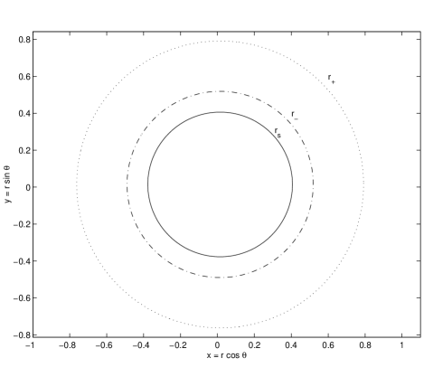
Figure 1: The singularity and horizons of the toroidal 3D space-time in the coordinates of metric (37). The parameters are such that the event horizon at $r_{+}$ (dotted line) and Cauchy horizon at $r_{-}$ (slash-dotted line) are present. Spacetime ends at the singularity $r_{s}$ (full line).

The horizons of (37) are given by the real roots of the equation

$$\alpha^{2}r^{4}-4m\left(1-\frac{3}{2}{a^{2}\alpha^{2}}\right)r+4(q^{2}+g^{2})\left(\frac{1-\frac{3}{2}a^{2}\alpha^{2}}{1-\frac{1}{2}a^{2}\alpha^{2}}\right)=0\,.$$ (54)

In the analysis of horizons, the relevant function is

$$Descr={3\over 4}(1-\frac{1}{2}{a^{2}\alpha^{2}})\sqrt[3]{(1-\frac{3}{2}{a^{2}\alpha^{2}})\,\frac{m^{4}}{\alpha^{2}}\,}-q^{2}-g^{2}$$ (55)

Depending on the relative values of mass $m$, charges $q$, $a$ and $g$, we have three distinct cases to analyze (the case $q^{2}+g^{2}=0$ is considered in next subsection): (i) $Descr>0$ – in such a case the metric (37) has two horizons, the event horizon at $r_{+}$ and the Cauchy or inner horizon at $r_{-}$. This is shown in Fig. 1. The singularity at $r=r_{s}$ is enclosed by both horizons. The spacetime can then be extended through the horizons till $r_{s}$. It represents a static black hole. Note that the other region between $r_{s}$ and $r=0$, belongs to a disconnected spacetime and we do not analyze it further; (ii) $Descr=0$ – the solution is the extreme black hole spacetime. There is only one horizon at $r=r_{+}=r_{-}=\sqrt[3]{m\left(1-\frac{3}{2}a^{2}\alpha^{2}\right)/\alpha^{2}}\,=\sqrt[4]{\frac{4}{3}\frac{(q^{2}+g^{2})}{\alpha^{2}}\left(\frac{1-\frac{3}{2}a^{2}\alpha^{2}}{1-\frac{1}{2}a^{2}\alpha^{2}}\right)\,}$. In such a case, when drawing an analog figure to Fig. 1, the dotted and the dashed (external) lines would coincide with each other, and the singularity at $r=r_{s}$ (solid internal line) would be still hidden (to external observers) by the horizon. Geodesic inward lines end at the singularity $r_{s}$; (iii) $Descr<0$ – this solution has no horizons and represents a naked singularity. From the above description, the Penrose diagrams, with the inherent topology and causal structure of spacetime, can easily be drawn.

III.2.3 Special cases

(a) The $J=0$ case

This case corresponds to an uncharged version of the solution studied in Sect. III.2.1, since $J=0$ implies $a=0$, what makes the Kaluza-Klein electric charge ${\cal Q}_{e}$ equal to zero. The magnetic charge $Q_{m}$ also vanish (see Eqs. (46) and (47)).

The 3D metric and other fields are obtained also by the dimensional reduction of the static charged 4D spacetime given by Eqs. (32) and (33), which yield,

$$ds^{2} = -\left(\alpha^{2}r^{2}-\frac{4m}{r}+\frac{4(q^{2}+g^{2})}{r^{2}}\right)d{{t}}^{2}+\frac{dr^{2}}{\alpha^{2}r^{2}-\frac{4m}{r}+\frac{4(q^{2}+g^{2})}{r^{2}}}+r^{2}d\theta^{2}\,,$$ (56)

$${\bf A} = -{2q\over r}\,{\rm\bf d}t\,,$$ (57)

$$L^{2}e^{2\beta_{1}\phi} = r^{2}\,,$$ (58)

$$\Psi = -{2g}\,\theta\,,$$ (59)

and the other fields vanish. This solution represents a 3D static spherically symmetric charged black hole whose geodesic and causal structures are the same as the $\varphi=$ constant plane of the 4D static toroidal black hole (32). Such a black hole has mass $m$, electric charge $q$ and an additional charge $g$, the source to the $\Psi$ scalar field. The dilaton charge is zero. The Ricci and Kretschmann curvature scalars are, respectively, $R=-6\alpha^{2}-{12(q^{2}+g^{2})\over r^{4}}$ and $K=12\alpha^{4}+{96m^{2}\over r^{6}}+{32\alpha^{2}(q^{2}+g^{2})\over r^{4}}-{512m(q^{2}+g^{2})\over r^{7}}+{704\left(q^{2}+g^{2}\right)^{2}\over r^{8}}$, showing that there is a singularity at $r=0$. For $q^{2}+g^{2}\leq{3\over 4}\sqrt[3]{\frac{m^{4}}{\alpha^{2}}\,}$ there are two horizons and the singularity is hidden to asymptotic external observers. On the other hand, if $q^{2}+g^{2}>{3\over 4}\sqrt[3]{\frac{m^{4}}{\alpha^{2}}\,}$ the singularity is naked.

(b) The uncharged $q^{2}+g^{2}=0$ case

An interesting 3D spherical black hole is obtained by the dimensional reduction of the 4D toroidal rotating uncharged black hole. Such a solution can also be obtained directly from (37)–(41) by putting $q=0$ and $g=0$. Namely,

$$ds^{2} = -{\alpha^{2}r^{2}-{4m\over r}\left(1-\frac{3}{2}a^{2}\alpha^{2}\right)\over 1+{4ma^{2}\over r^{3}}}\,dt^{2}+\frac{dr^{2}}{\alpha^{2}r^{2}-{4m\over r}\left(1-\frac{3}{2}a^{2}\alpha^{2}\right)}+r^{2}\,d\theta^{2}\,,$$ (60)

$${\bf{\cal A}} = -{4m\,a\sqrt{1-\frac{1}{2}a^{2}\alpha^{2}}\over r^{3}+4m\,a^{2}}\,L\,{\rm\bf d}t\,,$$ (61)

$$L^{2}e^{2\beta_{1}\phi} = r^{2}+{4m\,a^{2}\over r}\,,$$ (62)

with the other fields being identically zero. This solution corresponds to a 3D charged static black hole with just one gauge field whose electric charge is ${\cal Q}_{e}=\frac{3}{2}ma\sqrt{1-{1\over 2}a^{2}\alpha^{2}}$. The mass and angular momentum are the same as for the case $q^{2}+g^{2}\neq 0$. Singularities and horizons of this spacetime are also easily obtained from the solution studied in Sect. III.2.1 with $q^{2}+g^{2}=0$. For all possible values of parameters $\alpha^{2}>0$, $m(1-\frac{3}{2}a^{2}\alpha^{2})>0$ and $a^{2}(1-\frac{3}{2}a^{2}\alpha^{2})>0$, there is always just one horizon at $r=\sqrt[3]{4(1-\frac{3}{2}a^{2}\alpha^{2})\frac{m}{\alpha^{2}}\,}$, and a singularity at $r=0$.

(c) The $\alpha=0$ case

After dimensional reduction along the $\partial_{\varphi}$ direction the metric and the other potentials can be obtained directly by making $\alpha^{2}=0$ in Eqs. (37)–(41), which give

$$ds^{2} = -{\left[{-4m\over r}+{4(q^{2}+g^{2})\over r^{2}}\right]\over 1+{4ma^{2}\over r^{3}}-{4(q^{2}+g^{2})\,a^{2}\over r^{4}}}\,dt^{2}+\frac{dr^{2}}{{-4m\over r}+{4(q^{2}+g^{2})\over r^{2}}}+r^{2}d\theta^{2}\,,$$ (63)

$${\bf A} = -2{q\over r}\,{\rm{\bf d}}t\,,$$ (64)

$${\bf{\cal A}} = {a\left[-4mr-4(q^{2}+g^{2})\right]\over r^{4}+4ma^{2}r-4(q^{2}+g^{2})\,a^{2}}\,L\,{\rm\bf d}t\,,$$ (65)

$$L^{2}e^{2\beta_{1}\phi} = r^{2}+{4ma^{2}\over r}-{4(q^{2}+g^{2})a^{2}\over r^{2}}\,,$$ (66)

$$\Psi = {2q\over r}{a}-2\,g\,\theta\,.$$ (67)

We have two distinct cases. Indeed, if $q^{2}+g^{2}\neq 0$ there is one horizon, $r_{h}=(q^{2}+g^{2})/m$. On the other hand, if $q^{2}+g^{2}=0$ there are no horizons and the singularity is naked: in contrast to the 4D black holes with spherical horizons the 4D uncharged toroidal black holes vanish when the cosmological constant is set to zero, leaving a naked singularity. In both cases, the asymptotic region $r\longrightarrow\pm\infty$ is not well defined. We do not comment further on this case.

(d) The rotating black hole

One may, if one wishes, put this black hole to rotate by performing a forbidden coordinate transformation which mixes time and angles. This yields a new rotating solution.

III.3 The 3D black hole spacetime in other frames

Up to now we have analyzed the 3D black hole in the good frame. Once we have the metric in the good frame, the metric in any other frame can be obtained by the conformal transformation given in Eq. (17). We consider first the Einstein frame which follows by putting $(\beta_{0})_{\rm o}=-(\beta_{1})_{\rm o}$, or by using Eqs. (37) and (40) and choosing $\beta_{0}=-\beta_{1}$. This gives,

$$ds^{2}_{\rm E}=-\Delta\,d\bar{t}^{2}+\left(1-\frac{1}{2}a^{2}\alpha^{2}\over 1-\frac{3}{2}a^{2}\alpha^{2}\right)\left(\alpha^{2}\bar{r}^{4}-{a^{2}\alpha^{2}\over 1-\frac{1}{2}a^{2}\alpha^{2}}\,\Delta\right)\left(\frac{d\bar{r}^{2}}{\Delta}+d\bar{\theta}^{2}\right)\,,$$ (68)

where $\Delta$ is defined as before, and all the other fields keep the same form of Eqs. (40)–(41). We have dressed the coordinates with bars to make clear they are different from the metric in the good frame (37). This solution and (37) are conformally equivalent, except in the loci $r=0$ and $\Gamma(r)=r^{4}(1-\frac{1}{2}a^{2}\alpha^{2})-a^{2}\Delta(r)=0$, where the metric (37) is singular. Metric (68) presents horizons at points where $\Delta(\bar{r})=0$, and singularities when $\Gamma(\bar{r})=\bar{r}^{4}(1-\frac{1}{2}a^{2}\alpha^{2})-a^{2}\Delta(\bar{r})=0$. The charges for both of the metrics are also the same. Good and Einstein frames in this case both yield black holes.

Other frames can also be considered. For comparison, we show also the metric of the toroidal 3D black hole in the string frame. Once again, we start with the metric in the good frame and use Eq. (17), where now $\left({\beta_{0}\over\beta_{1}}\right)_{\!\rm o}=-(1\mp\sqrt{2})$, yielding

$$ds^{2}_{\rm s} = -\left[{r^{4}\left(1-\frac{1}{2}a^{2}\alpha^{2}\right)-a^{2}\Delta\over 1-\frac{3}{2}a^{2}\alpha^{2}}\,\right]^{\mp\sqrt{2}}\Delta\,dt^{2}+$$ (69)

$$\left[{r^{4}\left(1-\frac{1}{2}a^{2}\alpha^{2}\right)-a^{2}\Delta\over 1-\frac{3}{2}a^{2}\alpha^{2}}\,\right]^{1\mp\sqrt{2}}\left(\frac{dr^{2}}{\Delta}+d\theta^{2}\right)\,,$$

and all the other fields keep the same form of Eqs. (40)–(41). The string and Einstein frames are related by $ds^{2}_{\rm s}=\left(e^{-\phi}\right)_{\!{\rm E}}^{\mp\sqrt{2}}ds^{2}_{{}_{\rm E}}$, where $\left(e^{2\beta_{1}\phi}\right)_{\!{\rm E}}$ is the dilaton field in the Einstein frame where $\beta_{1}=-1/2$. Properties of the metric in the string and Einstein frames are very similar, with the same singularities and horizons. The conformal transformation relating the two frames is well defined everywhere except at points where $r^{4}(1-\frac{1}{2}a^{2}\alpha^{2})-a^{2}\Delta(r)=0$, which correspond to singularities of the spacetime.

III.4 The 2D black hole spacetime

One can reduce one more dimension. Our aim is now to go from the 3D black hole presented in Eqs. (37)–(41) to the corresponding 2D reduced black hole by performing a consistent truncation along the $\theta$ direction. In order to perform a consistent dimensional reduction we have to choose $g=0$ in Eqs. (38) and (41). The result is a (1+1)–dimensional black hole solution of gravity theory with two gauge fields $\bf A$ and $\cal A$, two dilaton $\phi_{1}$ and $\phi_{2}$, and with one scalar field $\Psi$:

$$e^{2(\beta_{0}\phi_{1}+\bar{\beta}_{0}\phi_{2})}ds^{2} = -{\left(1-\frac{3}{2}{a^{2}\alpha^{2}}\right)\,\Delta\over r^{2}(1-\frac{1}{2}{a^{2}\alpha^{2}})-{a^{2}\Delta\over r^{2}}}\,dt^{2}+r^{2}\frac{dr^{2}}{\Delta}\,,$$ (70)

$${\bf A} = -2{q\over r}\,{\rm\bf d}t\,,$$ (71)

$${\bf{\cal A}} = {a\left(\Delta-\alpha^{2}r^{4}\right)\over r^{4}(1-\frac{1}{2}{a^{2}\alpha^{2}})-a^{2}\Delta}\,L\,{\rm\bf d}t\,,$$ (72)

$$L^{2}e^{2\beta_{1}\phi_{1}} = {1\over 1-\frac{3}{2}{a^{2}\alpha^{2}}}\left[r^{2}\left(1-\frac{1}{2}{a^{2}\alpha^{2}}\right)-{a^{2}\Delta\over r^{2}}\right]\,,$$ (73)

$$e^{2\beta_{2}\phi_{2}} = r^{2}\,,$$ (74)

$$\Psi = {2q\over r}{a\over\sqrt{1-\frac{1}{2}{a^{2}\alpha^{2}}\,}}\,,$$ (75)

where $\beta_{0},\bar{\beta}_{0},\beta_{1},\beta_{2}$ are arbitrary constants. Even though this two-dimensional solution also presents interesting properties, it will not be studied in detail here. For the particular case with no charges and angular momentum see lemosCQG .

IV Conclusions

We have presented the dimensional reduction to 3D of the rotating charged toroidal-AdS black hole. Dimensional reduction, through the Killing azimuthal direction $\partial/\partial\varphi$, produced 3D black holes with an isotropic event horizon (i.e., circularly symmetric), and the new charges were neatly found.

There are other interesting classes of black holes in 4D to which this procedure could also be applied, namely the hyperbolic black holes mann ; peldan , as well as the toroidal-AdS holes found in klemm_mor_vanzo which are not isometric to those of lemos1 ; lz1 . Such an analysis can be done with the techniques presented here.

References

- (1) M. Bañados, C. Teitelboim, J. Zanelli, Phys. Rev. Lett. 69, 1849 (1992).
- (2) M. Bañados, M. Henneaux, C. Teitelboim, J. Zanelli, Phys. Rev. D 48, 1506 (1993).
- (3) S. Deser, R. Jackiw, G. ’t Hooft, Annals. Phys. 152, 220 (1984).
- (4) S. Deser, R. Jackiw, Annals Phys. 153, 405 (1984).
- (5) S. Giddings, J. Abbott, K. Kuchař, Gen. Rel. Grav. 16, 751 (1984).
- (6) A. Achúcarro, P. K. Townsend, Phys. Lett. B 180, 89 (1988).
- (7) E. Witten, Nucl. Phys. B 311, 46 (1988).
- (8) J. H. Horne, G. T. Horowitz, Nucl. Phys. B, 368, 444 (1992).
- (9) G. T. Horowitz, D. L. Welch, Phys. Rev. Lett. 71, 328 (1993).
- (10) S. Carlip, Class. Quantum Grav. 12, 2853 (1995).
- (11) J. P. S. Lemos, Phys. Lett. B 353, 46 (1995).
- (12) J. P. S. Lemos, V. T. Zanchin, Phys. Rev. D 54 3840 (1996).
- (13) P. M. Sá, A. Kleber, J. P. S. Lemos, Class. Quantum Grav. 13, 125 (1996).
- (14) O. J. C. Dias, J. P. S. Lemos, Phys. Rev. D 64, 064001 (2001).
- (15) K. C. K. Chan, R. B. Mann, Phys. Rev. D 50, 6385 (1994); (E) Phys. Rev. D 52, 2600 (1995).
- (16) M. Henneaux, C. Martínez, R. Troncoso, J. Zanelli, Phys. Rev. D 65, 104007 (2002).
- (17) D. Ida, Phys. Rev. Lett. 85, 3758 (2000).
- (18) J. Maldacena, Adv. Theor. Phys. 2, 231 (1998).
- (19) J. Maldacena, A. Strominger, J. High Energy Phys. 12, 005 (1998).
- (20) M. Duff, “TASI Lectures on Branes, Black Holes and Anti-de Sitter Space”, hep-th/9912164.
- (21) G. T. Horowitz, “The Dark Side of String Theory: Black Holes and Black Strings”, hep-th/9210119.
- (22) M. J. Duff, B. E. W. Nilsson, C. N. Pope, Phys. Rept. 130, 1 (1986).
- (23) E. Cremmer, in Supergravity 81, eds. S. Ferrara, J. G. Taylor (Cambridge University Press, 1982).
- (24) P. Breitenlohner, D. Maison, G. Gibbons, Commun. Math. Phys. 120, 295 (1988).
- (25) A. Ashtekar, J. Bičák, B. G. Schmidt, Phys. Rev. D 55, 669 (1997).
- (26) K. S. Stelle, “Lectures on Supergravity p-branes”, hep-th/9701088.
- (27) K. C. K. Chan, J. D. E. Creighton, R. B. Mann, Phys. Rev. D 54, 3892 (1996).
- (28) D. Marolf, “String/M-branes for Relativists”, gr-qc/9908045.
- (29) J. D. Brown, J. W. York, Phys. Rev. D 47, 1407 (1993).
- (30) J. D. Brown, J. D. E. Creighton, R. B. Mann, Phys. Rev. D 50, 6394 (1994).
- (31) J. D. E. Creighton, R. B. Mann, Phys. Rev. D. 52, 4569 (1995).
- (32) M. Henneaux, C. Teitelboim, Phys. Rev. Lett. 56, 689 (1986).
- (33) R. Pisarski, Phys. Rev. D 34, 3851 (1986).
- (34) E. W. Hirschmann, D. L. Welch, Phys. Rev. D 53, 5579 (1996).
- (35) O. J .C. Dias, J. P. S. Lemos, J. High Energy Phys. 01, 006 (2002).
- (36) W. A. Moura-Melo, J. A. Helayël-Neto, Phys. Rev. D 63, 065013 (2001); E. M. C. Abreu, J. A. Helayël-Neto, M. Hott, W. A. Moura-Melo, Phys. Rev. D 65, 085024 (2002).
- (37) I. S. Booth, R. B. Mann, Phys. Rev. D 60, 124009 (1999).
- (38) D. Garfinkle, G. T. Horowitz, A. Strominger, Phys. Rev. D 43, 3140 (1991).
- (39) G. W. Gibbons, M. J. Perry, Int. J. Mod. Phys. D 1, 335 (1992).
- (40) R. Kallosh, A. Linde, T. Ortín, A. Peet, A. Van Proeyen, Phys. Rev. D 46 5278 (1992).
- (41) J. P. S. Lemos, Class. Quantum Grav. 12, 1081 (1995).
- (42) R. B. Mann, Class. Quantum Grav. 7, 219 (1997).
- (43) S. Åminneborg, I. Bengtsson, S. Holst, P. Peldán, Class. Quantum Grav. 13, 2707 (1996).
- (44) D. Klemm, V. Moretti, L. Vanzo, Phys. Rev. D 57, 6127 (1998).