Fake signals caused by heavy mass motions near a sensitive spherical gravitational wave antenna

Abstract

This paper analyses in quantitative detail the effect caused by a moving mass on a spherical gravitational wave detector. This applies to situations where heavy traffic or similar disturbances happen near the GW antenna. Such disturbances result in quadrupole tidal stresses in the antenna mass, and they therefore precisely fake a real gravitational signal. The study shows that there always are characteristic frequencies, depending on the motion of the external masses, at which the fake signals are most intense. It however appears that, even at those frequencies, fake signals should be orders of magnitude below the sensitivity curve of an optimised detector, in likely realistic situations.

1 Introduction

Large mass spherical gravitational wave (GW) detectors [1, 2] constitute sensitive systems with a real promise of sighting GW events in the frequency range of 1 kHz, even with a rather large bandwidth [3]. In such extremely delicate device as an acoustic GW detector is [4, 5, 6, 7, 8], any disturbance, whether internal or external, must be considered and, if possible, screened out both in hardware and in software [9, 10]. Quite recently, a possibility has arisen to build an underground spherical detector in the Spanish Pyrinees [11], located near a road tunnel.

Heavy traffic in the tunnel is there almost at all times. It is therefore important to assess the effect of the passing vehicles close to the antenna. Purely Newtonian action is expected on the sphere which exactly fakes a real GW signal, since it shows up as a local tide, with its characteristic quadrupole structure. Hope is that such fake signals be weak compared to actual GW signals. Otherwise, even if veto control on them could easily be exercised, an almost continuous background of spurious signals would contaminate the detector output, eventually concealing a real signal.

The purpose of this paper is to calculate the effect of traffic on the spherical detector by means of a point moving mass model, and to present the results of applying the theory to a realistic situation. We shall first consider the effect of a mass moving with uniform speed past the detector. As we shall see, this causes a very small impact on the detector in any reasonable circumstances, and we thus consider next the effect of oscillating parts in the passing vehicle, which can be more important. In section 2 we pose the general problem, then in sections 3 and 4 we fully consider each case; section 5 is finally devoted to comment on the results obtained and their practical relevance in a real detector site.

2 The problem

The situation is best described by the schematic graphic displayed in figure 1: a spherical GW detector has its centre at the origin of coordinates, and a moving mass $m\/$ travels in a straight line past the detector with a given impact parameter $|\bi{d}|$. We shall assume that the detector’s radius $R\/$ is much smaller than this parameter, i.e.,

$$R\ll|{\bi{d}}|\;,$$ (1)

and ask which is the Newtonian gravitational action of the moving mass on the GW detector.

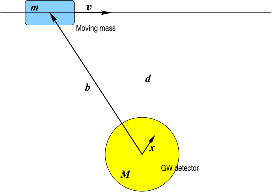
Figure 1: Schematics of a passing mass and a spherical GW detector. Distances do not match the scales of any realistic example.

Let then $\phi(\bi{x},t)$ be the gravitational potential generated by the moving mass at point $\bi{x}$ at time $t$. We shall of course assume it satisfies Poisson’s equation

$$\nabla^{2}\phi(\bi{x},t)=-4\pi G\,\rho(\bi{x},t)$$ (2)

where $G\/$ is Newton’s constant, and $\rho(\bi{x},t)$ is the mass density distribution of the moving mass. We shall also assume this sufficiently small that it can be considered a point mass, i.e.,

$$\rho(\bi{x},t)=m\,\delta^{(3)}(\bi{x}-\bi{b})$$ (3)

where (see again figure 1)

$$\bi{b}=\bi{b}(t)=\bi{d}+\bi{v}t$$ (4)

if one adopts the (arbitrary) convention that the moving mass crosses the point of closest distance to the detector, $\bi{d}$, at time $t=0$, and that it moves with constant velocity $\bi{v}$. The gravitational potential is thus

$$\phi(\bi{x},t)=-\frac{Gm}{|\bi{x}-\bi{b}(t)|}$$ (5)

GWs show up in the detector as local tides, therefore the moving mass will cause signal confusion inasmuch as it too produces tides. Under the assumption (1) above, we can calculate the gravitational potential inside the sphere by the approximate expansion

$$\phi(\bi{x},t)=\phi({\bf 0},t)+\partial_{i}\phi({\bf 0},t)\,x_{i}+\mbox{\Large$\frac{1}{2}$}\;\partial_{i}\partial_{j}\phi({\bf 0},t)\,x_{i}x_{j}+\ldots$$ (6)

The gravitational accelerations are correspondingly given by the gradient of the potential, i.e., $\bi{a}$ = $-\nabla\phi$, or

$$a_{i}(\bi{x},t)=-\partial_{i}\phi({\bf 0},t)\,x_{i}-\partial_{i}\partial_{j}\phi({\bf 0},t)\,x_{j}+\ldots$$ (7)

The first term in the rhs represents the global pull on the sphere, and cannot therefore excite its oscillation modes; these are instead excited by the acceleration gradients, or tides, given by the second term. These acceleration gradients can be converted to a density of forces (force per unit volume) simply by multiplying them by the density of the sphere, $\varrho$, say, to obtain

$$f_{i}^{\rm MM}(\bi{x},t)=-\varrho\;\partial_{i}\partial_{j}\phi({\bf 0},t)\,x_{j}\equiv\varrho\,R_{ij}^{\rm MM}(t)\,x_{j}$$ (8)

We readily find

$$R_{ij}^{\rm MM}(t)=-\frac{3Gm}{b^{3}(t)}\;\left(\frac{b_{i}(t)\,b_{j}(t)}{b^{2}(t)}-\frac{1}{3}\,\delta_{ij}\right)$$ (9)

where $b(t)\equiv|\bi{b}(t)|$. The interaction of the passing mass with the sphere is described by the usual equations of elasticity theory [12]

$$\varrho\,\frac{\partial^{2}\bi{u}}{\partial t^{2}}-\mu\nabla^{2}\bi{u}-(\lambda+\mu)\,\nabla(\nabla{\bf\cdot}\bi{u})=\bi{f}(\bi{x},t)\;.$$ (10)

The structure of $\bi{f}^{\rm MM}(\bi{x},t)$ is obviously purely quadrupole, so it can be split up much in the same way as a GW excitation:

$$\bi{f}^{\rm MM}(\bi{x},t)=\sum_{m=-2}^{2}\,\bi{f}^{(m)}(\bi{x})\,C^{(m)}(t)$$ (11)

where

$$f_{i}^{(m)}(\bi{x})=\varrho\,E_{ij}^{(2m)}\,x_{j}\ ,\qquad C^{(m)}(t)=\frac{8\pi}{15}\,E_{ij}^{*(2m)}\,R_{ij}^{\rm MM}(t)$$ (12)

with $m=-2,\ldots,2$. The matrices $E_{ij}^{(2m)}$ are given by [1]

$$E_{ij}^{(20)} = \left(\mbox{\large$\frac{5}{16\pi}$}\right)^{\!\frac{1}{2}}\left[\begin{array}[]{ccc}-1&0&0\\ 0&-1&0\\ 0&0&2\end{array}\right]$$ (13d)

$$E_{ij}^{(2\pm 1)} = \left(\mbox{\large$\frac{15}{32\pi}$}\right)^{\!\frac{1}{2}}\left[\begin{array}[]{ccc}0&0&\mp 1\\ 0&0&-i\\ \mp 1&-i&0\end{array}\right]$$ (13h)

$$E_{ij}^{(2\pm 2)} = \left(\mbox{\large$\frac{15}{32\pi}$}\right)^{\!\frac{1}{2}}\left[\begin{array}[]{ccc}1&\pm i&0\\ \pm i&-1&0\\ 0&0&0\end{array}\right]\;.$$ (13l)

The sphere’s response to the forces (11) is thus determined by the series expansion

$$\bi{u}^{\rm MM}(\bi{x},t)=\sum_{n=1}^{\infty}\,\frac{a_{n2}}{\omega_{n2}}\,\left[\sum_{m=-2}^{2}\,\bi{u}_{n2m}(\bi{x})\,C_{n2}^{(m)}(t)\right]$$ (13n)

which is formally identical to the response to a GW excitation . Our concern is now to compare this with the system’s response to a real GW. We come to it in the next section.

3 Equivalent signal

A meaningful comparison between the passing mass fake signal and an actual GW signal is best set up in frequency domain, as it is in this form that the detector’s sensitivity is defined.

Consider first a point on the sphere’s surface, $\bi{x}=R\bi{n}$, where $\bi{n}$ is a unit outward pointing normal, and calculate its radial displacement $u(t)$, i.e.,

$$u(t)\equiv\bi{n}\cdot\bi{u}(R\bi{n},t)\;.$$ (13o)

Because of the form of the sphere’s wavefunctions, the Fourier transform of the above is easily seen to be [3]

$$\tilde{u}^{\rm GW}(\omega)=-\frac{1}{2}\sum_{n=0}^{\infty}a_{n2}A_{n2}(R)\,\omega^{2}\tilde{h}(\omega)\,L_{n2}(\omega)\;,$$ (13p)

where $L_{n2}(\omega)$ is the mode’s transfer function

$$L_{n2}(\omega)=\frac{1}{-\omega^{2}+2i\gamma_{n2}\;\omega+\omega_{n2}^{2}}$$ (13q)

with $\gamma_{n2}$ the linewidth of the mode, and $\tilde{h}(\omega)$ the Fourier transform of the signal $h(t)$, defined by

$$h(t)\equiv h_{ij}(t)\,n_{i}n_{j}$$ (13r)

Likewise, the radial displacement induced at the same location of the sphere by the moving mass is easily inferred from equation (13n):

$$\tilde{u}^{\rm MM}(\omega)=\sum_{n=0}^{\infty}a_{n2}A_{n2}(R)\,\tilde{R}_{ij}^{\rm MM}(\omega)\,n_{i}n_{j}\,L_{n2}(\omega)$$ (13s)

We can at this point define an equivalent amplitude associated to the fake moving mass signal; the natural definition is [3]:

$$\left|\tilde{h}_{\rm equiv}^{\rm MM}(\omega)\right|^{2}\equiv\frac{\left|\tilde{u}^{\rm MM}(\omega)\right|^{2}}{\left|\tilde{u}^{\rm GW}(\omega)\right|^{2}/|\tilde{h}(\omega)|^{2}}$$ (13t)

We thus find

$$\left|\tilde{h}_{\rm equiv}^{\rm MM}(\omega)\right|^{2}=4\omega^{-4}\,\left|\tilde{R}_{ij}^{\rm MM}(\omega)\,n_{i}n_{j}\right|^{2}\;.$$ (13u)

It is important to stress here that this expression holds for solid spheres as well as for hollow spheres, and indeed for a dual sphere, too. This is simply because the mode expansion is identical in the GW signal and in the passing mass signal.

An order of magnitude estimate of the passing mass equivalent signal is accomplished by replacing $\left|\tilde{R}_{ij}^{\rm MM}(\omega)\,n_{i}n_{j}\right|^{2}$ in equation (13u) with $\left[\tilde{R}_{ij}^{*{\rm MM}}(\omega)\tilde{R}_{ij}^{\rm MM}(\omega)\right]$, i.e.,

$$\left|\tilde{h}_{\rm equiv}^{\rm MM}(\omega)\right|^{2}\leq 4\omega^{-4}\;\tilde{R}^{*{\rm MM}}_{ij}(\omega)\tilde{R}_{ij}^{\rm MM}(\omega)\;,$$ (13v)

The Fourier transforms $\tilde{R}_{ij}^{\rm MM}(\omega)$ are expediently calculated adopting a coordinate system where the $x\/$-axis is parallel to the velocity vector $\bi{v}$, and the $y\/$-axis is in the direction of the vector $\bi{b}$ of figure 1. The result is

$$\tilde{R}_{ij}^{\rm MM}(\omega)=\frac{Gm}{vd^{2}}\,\left(\begin{array}[]{ccc}z^{2}K_{2}(z)-2zK_{1}(z)&-iz^{2}K_{1}(z)&0\\ -iz^{2}K_{1}(z)&-z^{2}K_{2}(z)+zK_{1}(z)&0\\ 0&0&zK_{1}(z)\end{array}\right)$$ (13w)

where $d\equiv|\bi{d}|$, and

$$z\equiv\omega/\omega_{0}\ ,\qquad\omega_{0}\equiv\frac{v}{d}$$ (13x)

with the $K\/$’s representing modified Bessel functions [13]:

$$K_{\nu}(z)=\frac{\Gamma\left(\nu+1/2\right)}{\Gamma\left(1/2\right)}\,\left(\frac{2}{z}\right)^{\!\nu}\;\int_{0}^{\infty}\;\frac{\cos zt}{(1+t^{2})^{\nu+1/2}}\,dt\;.$$ (13y)

It is now easily seen that

$$\left|\tilde{h}_{\rm equiv}^{\rm MM}(\omega)\right|\leq\frac{Gm}{vd^{2}}\;\omega^{-2}\,f(z)$$ (13z)

where

$$f(z)\equiv\left[z^{4}K_{2}^{2}(z)+(3+z^{2})\,z^{2}K_{1}^{2}(z)-3z^{3}K_{1}(z)K_{2}(z)\right]^{1/2}\;.$$ (13aa)

This function has asymptotic behaviours:

$$f(z) \sim 1+\left(\frac{z}{2}\right)^{\!2}\ ,\ \ \qquad{\rm if}\ \ z\ll 1$$ (13ab)

$$f(z) \sim \sqrt{\pi}\,z^{3/2}\,e^{-z}\ ,\qquad{\rm if}\ \ z\gg 1\;,$$ (13ac)

and has a rather smooth maximum at $z\sim 1$, as we see in the plot of figure 2.

The salient feature of $f(z)$ as regards our present concern is however its exponential roll-off in the high frequency range. Take for example as reasonable figures a somewhat fast 10 ton truck travelling at a speed of 40 m/s ($\sim$ 140 km/h), with an impact parameter $d$ = 80 m; this gives a frequency $v/d$ = 0.5 rad/sec, or $\sim$ 0.1 Hz, which means we must go up to $z\sim 10^{4}$ for frequencies in the kHz range, where a spherical detector will be sensitive. But this produces an utterly meaningless $\tilde{h}_{\rm equiv}^{\rm MM}\sim 10^{-4354}$ at $\omega/2\pi$ = 1 kHz …

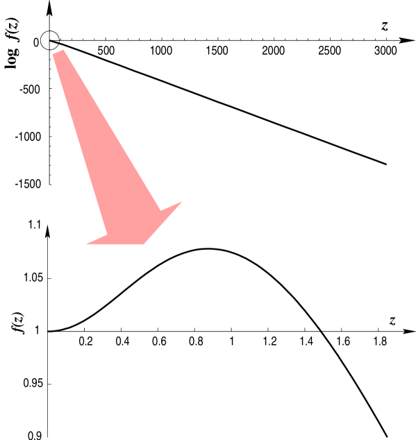
Figure 2: Above: the spectral density function $f(z)$ of equation (13aa), plotted on a logarithmic scale. Below: close-up of the above in the low frequency range, showing the function’s maximum at $z\simeq 0.88$. Linear scales have been used here for clarity.

Such number clearly indicates that anything will produce more substantial fake signals in the detector, provided it has some vigor in the kHz range. An example could be e.g. internal motions of parts of the vehicle, such as the engine pistons, which undergo periodic oscillations of a more appreciable magnitude. We come to this next.

4 Periodic source

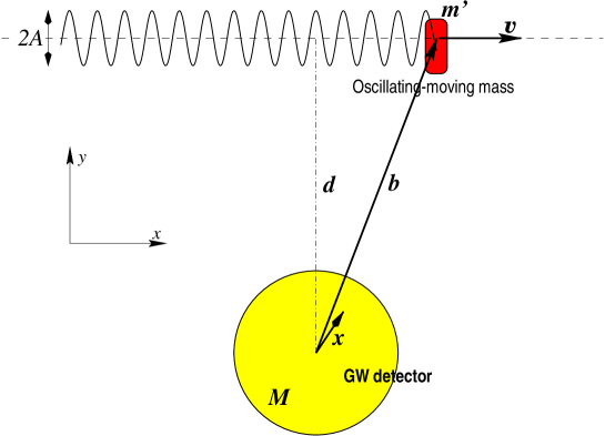
Figure 3: Schematics of a spherical GW detector and a passing mass which, simultaneously, oscillates with amplitude $A$. Again, distances do not match realistic scales.

Consider thus that certain internal parts of the passing vehicle oscillate with (angular) frequency $\alpha$ and amplitude $A$ —see figure 3. If we represent with $m^{\prime}$ the mass of one such part then the Newtonian potential at a field position $\bi{x}$ relative to the detector’s centre is obviously given by

$$\phi(\bi{x},t)=-\frac{Gm^{\prime}}{|\bi{x}-\bi{b}(t)-\bi{c}(t)|}$$ (13ad)

where

$$\bi{b}(t)=(vt,0,0)\ ,\qquad\bi{c}(t)=(0,A\cos\alpha t,0)$$ (13ae)

with the axes convention shown in figure 3. The system response will be given in this case by the same formulas of section 2, except that the quadrupole matrix $R_{ij}^{\rm MM}(\omega)$ needs to be replaced with

$$R_{ij}^{\rm OMM}(t)=-\frac{3Gm^{\prime}}{|\bi{b}(t)+\bi{c}(t)|^{3}}\;\left(\frac{[b_{i}(t)+c_{i}(t)]\,[b_{j}(t)+c_{j}(t)]}{|\bi{b}(t)+\bi{c}(t)|^{2}}-\frac{1}{3}\,\delta_{ij}\right)$$ (13af)

and, in particular, the new equivalent signal will be given by

$$\left|\tilde{h}_{\rm equiv}^{\rm OMM}(\omega)\right|^{2}\leq 4\omega^{-4}\;\tilde{R}^{*{\rm OMM}}_{ij}(\omega)\tilde{R}_{ij}^{\rm OMM}(\omega)\;,$$ (13ag)

by the same arguments which led to equation (13v).

The Fourier transforms of the functions $R_{ij}^{\rm OMM}(t)$ in equation (13af) are too complicated to be performed analytically, but there are certain features which can be easily inferred by inspection of the defining formulas. Take for example the gravitational potential given by equation (13ad); we can recast this in the form

$$\phi(\bi{x},t)=-\frac{Gm^{\prime}}{|\bi{x}-\bi{b}|}\,\left[1-\frac{2\bi{c}\cdot(\bi{x}-\bi{b})}{|\bi{x}-\bi{b}|^{2}}+\frac{|\bi{c}|^{2}}{|\bi{x}-\bi{b}|^{2}}\right]^{-1/2}$$ (13ah)

and perform a power series expansion of the term in square brackets in the rhs on the basis that

$$|\bi{c}|\ll|\bi{x}-\bi{b}|$$ (13ai)

i.e., actually assuming that the amplitude $A$ of oscillations of the mass $m^{\prime}$ is much smaller than the impact parameter $|\bi{d}|$ —see figure 3. The series expansion will thus consist in a series of ascending powers of $|\bi{c}|=A\cos\alpha t$, so it will consequently involve all the harmonics of the frequency $\alpha/2\pi$, clearly with an amplitude which decreases with the harmonic order due to the inequality (13ai). Clearly, the same harmonic structure carries over to the higher derivatives of the potential, and in particular to the quadrupole moments $R_{ij}^{\rm OMM}(t)$.

Since we must give up the analytic approach of section 3, we shall now estimate the Fourier transforms $\tilde{R}_{ij}^{\rm OMM}(\omega)$ by numerical methods. For this we shall make the rather natural choice of using Fast Fourier Transform algorithms [14].

In this approach, first thing we need is to define an appropriate bandwidth to do the analysis. Our standard reference will be a dual sphere GW detector, which is the best spherical GW antenna we can think of at present —see [3]. To accurately match that reference we must assess the signal intensities up to a frequency of 3000 Hz, hence we need a bandwidth of 6000 Hz, including of course negative frequencies. We shall thus approximate Fourier transforms by DFT sums:

$$\tilde{R}_{ij}^{\rm OMM}(\omega_{n})=\Delta t\;\sum_{m=0}^{N-1}\,R_{ij}^{\rm OMM}(m\,\Delta t)\,e^{2\pi inm/N}\ ,\qquad\omega_{n}=n\Omega_{\rm Nyq}/N\;,$$ (13aj)

where $N\/$ is the total number of sample points, $\Omega_{\rm Nyq}$ is the Nyquist, or sampling frequency, and $\Delta t$ is the time interval between successive samples, i.e.,

$$\Delta t=\frac{2\pi}{\Omega_{\rm Nyq}}\;.$$ (13ak)

We now use the expansion (13aj) to determine the equivalent signal (13ag). The result is plotted in figure 4, where a dual sphere sensitivity curve has been added to assess the real effect of two instances of fake signals.

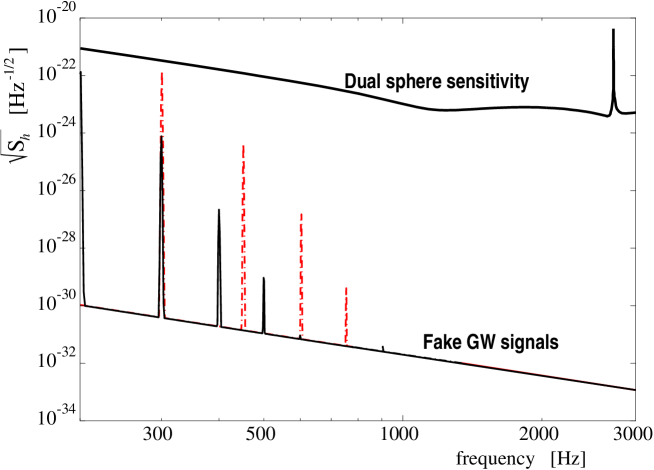
Figure 4: GW equivalent signal generated by an oscillating passing by mass, and sensitivity curve of a dual sphere GW detector as considered in reference [3]. The black solid line corresponds to a mass oscillating at 100 Hz, while the the red dash-dotted line corresponds to a faster oscillator of 150 Hz. The plot very clearly shows that the signal generated by these sources is orders of magnitude away from being detectable.

The graphic very clearly shows how far the effect is from causing a problem for gravitational wave physics, even though rather exaggerated data have been assumed in both of the instances plotted. These are the figures used in the plot:

Impact parameter:		$d\/$ = 50 metres
Horizontal speed:		$v\/$ = 40 m/s   ($\sim$ 140 km/h)
Oscillating mass:		$m^{\prime}\/$ = 100 kg
Oscillation amplitude:		$A\/$ = 40 cm

and the frequencies of oscillation are 100 Hz (6000 rpm) and 150 Hz (9000 rpm) in each of the examples, respectively. The results shown in the graph scale with the tabulated values as

$$\tilde{h}_{\rm equiv}\propto\frac{m^{\prime}A}{vd^{3}}\;,$$ (13al)

while it is also seen that narrow peaks happen at the harmonic frequencies of 100 Hz or 150 Hz —actually of $\alpha/2\pi$, as discussed above.

5 Concluding remarks

The calculations in this paper show that there is no practical possibility that noise generated by nearby traffic, which exactly fakes quadrupole GW noise, disturbs GW astronomy in the sensitivity band of the spherical detector, even if this is chosen as the best possible dual sphere system.

While this is particularly clear in the presented plots, we must still stress that those results actually constitute upper bounds on the fake signals, due to inequalities (13z) and (13ag). In addition, emphasis should also be put on the fact that most of the background signal we see in figure 4 is due to aliasing of the out-of-band frequency components.

Altogether then, it appears that installation of a very sensitive spherical GW detector in a site only a few hundred metres from a heavy traffic road is definitely not going to represent a problem for the system performance.

References

References

- [1] J.A. Lobo, Phys Rev D 52, 591 (1995), and J.A. Lobo, Mon Not Roy Astr Soc 316, 173 (2000). See also W.W. Johnson and S.M. Merkowitz, Phys Rev Lett 70, 2367 (1993)
- [2] E. Coccia, J.A. Lobo and J.A. Ortega, Phys Rev D 52 3735 (1995)
- [3] M. Cerdonio, L. Conti, J.A. Lobo, A. Ortolan, L. Taffarello and J.P. Zendri, Phys Rev Lett 87 031101 (2001)
- [4] P. Astone et al., Phys Rev D 47 362 (1993)
- [5] W.O. Hamilton et al., in First Edoardo Amaldi Conference on Gravitational Waves, edited by E. Coccia, G. Pizzella F. and Ronga, World Scientific Publishing Co., Singapore (1995)
- [6] I.S. Heng, D.G. Blair, E.N. Ivanov and M.E. Tobar, Phys Lett A 218 90 (1996)
- [7] P. Astone et al., Astropart Phys 7 231 (1997)
- [8] M. Cerdonio et al., Class Quant Grav 14 1491 (1997)
- [9] L. Baggio et al., Phys Rev D 61 102001 (2000)
- [10] Z.A. Allen et al., Phys Rev Lett 85 5046 (2000)
- [11] A. Morales, private communication (2002)
- [12] L.D. Landau, and E.M. Lifshitz, Theory of Elasticity, Pergamon (1970)
- [13] M. Abramowitz, and I.A. Stegun, Handbook of Mathematical Functions, Dover (1972)
- [14] See e.g. R. Tolimieri, M. An, and C. Lu, Mathematics of Multidimensional Fourier Transform Algorithms, Springer-Verlag (New York, 1993)