Derivation of the General Case Sagnac
Result using Non-time-orthogonal Analysis

Abstract

The Sagnac time delay and fringe shift dependency on angular velocity and enclosed area are derived from the rotating reference frame using non-time-orthogonal (NTO) tensor analysis. NTO analysis differs from traditional approaches by postulating that the continuous and single valued nature of physical time constrains simultaneity in a rotating frame to be unique (and thus not a matter of convention.) This implies anisotropy in the physical, local speed of light and invalidity of the hypothesis of locality for NTO frames. The Sagnac relationship for the most general case, in which the area enclosed is not circular and does not have the axis of rotation passing through its center, is determined.

Key words: Sagnac, relativistic rotation, non-time-orthogonal, speed of light, simultaneity.

1 INTRODUCTION

In 1913 M. G. Sagnac[1] sent light rays in the clockwise (cw) and counterclockwise (ccw) directions on a rotating platform, and examined the resulting interference fringe patterns made by the returning rays. He found, as have subsequent researchers, that the fringes shifted as the angular velocity of the platform changed. Post[2] summarized the results of these researchers and presented the experimentally determined first order relationship

$$\Delta Z=\frac{\Delta\lambda}{\lambda_{0}}=\frac{4\mbox{\boldmath$\omega$}\cdot\mbox{\boldmath$A$}}{c\lambda_{0}},$$ (1)

where $\omega$ and A are angular velocity and area vector quantities, respectively, $c$ is the standard value for speed of light in vacuum/air, and $\Delta Z$ is the fractional change in fringe location. $\lambda_{o}$ is wavelength of the light in the lab frame before it is directed down the axis of rotation, out a radial direction on the rotating platform, and split via a 50% reflection/transmission mirror into the two cw and ccw rays. In the simplest case where the two rays travel circular paths $A=$2$\pi r$ and $\omega=v/r$.

From the standpoint of special relativity theory (SRT), this result may seem perplexing, as SRT posits that no change in speed of the reference frame should affect the speed of light or any measurements that one could make. This principle is considered, via the hypothesis of locality (sometimes “the surrogate frames posulate”), to extend to general relativity (GR) in which (for the Einstein synchronization of SRT) the local physically measured one-way speed of light is $c$, even in non-inertial frames.

The hypothesis of locality, a linchpin in the traditional approach to relativistic rotation, states that a local inertial observer is equivalent to a local co-moving non-inertial observer in matters having to do with measurements of distance and time. (See Møller[3], Einstein[4], and Mashoon[5].) It follows immediately that a Lorentz frame can be used as a local surrogate for the non-inertial frame, and in such a frame (with Einstein synchronization), the local, measured, one-way speed of light is $c$.

Minguzzi[6] and Møller[7], among others, note that the hypothesis of locality is only an assumption. It is, however, an assumption that, historically, has worked very well in a large number of applications.

Given the foregoing, experiments performed in non-inertial frames, like those in inertial frames, should not have results dependent on the speed of the experimenter. Yet in the Sagnac experiment, the result depends on the speed $v$ of the platform along the path traveled by the rays.

Consider, for example, that the cw and ccw light rays travel identical routes (in reverse), and according to SRT (and GR) each must have the same speed $c$ as physically measured locally at all points along that path regardless of the motion of the platform. Hence, it seems one could only conclude that wave maxima (or minima) on both rays should return to the fringe location at the same time, regardless of path speed $v$, in apparent disagreement with the Sagnac result.

One may at first consider that the light rays originated from one source in the lab and that as they struck the half silvered mirrors and were reflected in opposite directions, they may have undergone Doppler shifting, which resulted in the observed effect[8]. However, Dufour and Prunier[9] carried out a series of experiments with the light source located on the platform itself and found no change in observed results.

Furthermore, the thought experiment of Appendix A demonstrates that short light pulses emitted from the same point on the platform, traveling the same path in the cw and ccw directions, must necessarily arrive back at that point at different times. Thus, any observer at that point would seem constrained to the conclusion that light, as seen from a rotating frame, travels at different speeds in the cw and ccw directions.

From the lab frame, derivation of the arrival time difference between the cw and ccw light pulses is well known[10]^,[11]^,[12] (summarized, for reference, in Appendix B), and from it, (1) readily results (see Section 4.1.) From the rotating frame, however, the situation is less clear. If one insists on the speed of light being locally invariant and isotropic, then it is not readily deduced that the cw and ccw rays arrive back at the emission point at different times.

Selleri[10] has made this derivation from the rotating frame, but only by denying the invariance of one way light speed in inertial frames, and thus effectively dismantling relativity theory as we know it. Others[11]^,[12]^,[13]^,[14] have based a derivation on local invariant/isotropic light speed, and a “desynchronization of clocks”. A satisfactory description of that approach is beyond the scope of this article, though the author suggests it is inappropriate physically. In his opinion, it leads to a discontinuity in physical time, clocks out of synchronization with themselves, and an arbitrary number of possible time readings on the same standard clock in the same coordinate frame for the same event. (See Klauber[15]^,[16].)

The present author has carried out an analysis of rotating frames[15]^,[16], similar in some aspects to an earlier and less extensive analysis by Langevin[17], using the metric obtained from the most commonly accepted transformation between the lab and the rotating frame. This metric has off diagonal time-space components and implies a non-orthogonality between time and space in rotating frames, dubbed by the author “non-time-orthogonality”.

That metric has been used successfully in the global positioning system (GPS) to account for time delays that would not be predicted under the usual relativistic assumption of isotropic local light speed. In fact Neil Ashby, recognized leader in GPS analysis, notes “ .. the principle of the constancy of c cannot be applied in a rotating reference frame ..”[18]. He also states “Now consider a process in which observers in the rotating frame attempt to use Einstein synchronization (constancy of the speed of light) ….. Simple minded use of Einstein synchronization in the rotating frame … thus leads to a significant error”.[19]

In non-time-orthogonal (NTO) analysis, one does not insist on transforming to local time orthogonal frames on the rotating platform, as is common among prior researchers. Instead, one simply examines the NTO metric and from it, deduces concomitant physical world behavior. When this is done, not only can the Sagnac effect be derived (as shown below), but all other observed rotating frame effects can be, as well. (See Klauber[15]^,[16]^,[20]^,[21]^,[22]^,[23]^,[24]^,[25].) Further, the geometric foundation of relativity theory remains intact. All general and special relativity analyses for time orthogonal frames are unchanged. That is, NTO analysis reduces to the traditional form when time is orthogonal to space.

2 SYNOPSIS OF NTO ANALYSIS

2.1 NTO Transformation and Metric

As shown in references [17], [15] and elsewhere, the rotating (NTO) frame metric can be derived using the most widely accepted transformation from the non-rotating (lab, upper case symbols) frame to a rotating (lower case) frame, i.e.,

$$\begin{array}[]{l}cT=ct\\ R=r\\ \Phi=\phi+\omega t\\ Z=z\\ \end{array}$$ (2)

where $\omega$ is the angular velocity of the rotating frame and cylindrical spatial coordinates are used. The coordinate time $t$ for the rotating system equals the proper time of a standard clock located in the lab. The ultimate viability of this transformation rests on its capability to predict real world phenomena, as discussed at length in reference [15].

Substituting the differential form of (2) into the line element in the lab frame

$$ds^{2}\mbox{ }=\mbox{ }-\mbox{ }c^{2}dT^{2}+\mbox{ }dR^{2}\mbox{ }+\mbox{ }R^{2}d\Phi^{2}\mbox{ }+\mbox{ }dZ^{2}$$ (3)

results in the line element for the rotating frame

$$ds^{2}\;\;=\;-c^{2}(1-\textstyle{{r^{2}\omega^{2}}\over{c^{2}}})dt^{2}\;+\;dr^{2}\;+\;r^{2}d\phi^{2}\;+\;2r^{2}\omega d\phi dt\;+\;dz^{2}=\;g_{\alpha\beta}dx^{\alpha}dx^{\beta}.$$ (4)

Note that the metric in (4) is not diagonal, since $g_{\phi t}\neq 0$, and this implies that time is not orthogonal to space (i.e., an NTO frame.)

2.2 Time in the Rotating Frame

Time on a standard clock at a fixed 3D location on the rotating disk, found by taking ds${}^{2}=-c^{2}d\tau$ and dr = d$\phi$ = dz = 0, is

$$d\tau=\sqrt{1-r^{2}\omega^{2}/c^{2}}dt=\sqrt{-g_{tt}}dt,$$ (5)

where dt here indicates coordinate time passed at the same 3D location.

More generally, the coordinate time difference between two events at two infinitesimally separated locations on the disk (each having its own clock), in coordinate components, is dt, where at least one of dr, d$\phi$, dz is not zero. The corresponding physical time difference (i.e., time difference measured between two different standard clocks fixed in the rotating frame) in seconds can be found from dt via the method described in Appendix C. It is

$$dt_{phys}=d\hat{t}=\sqrt{-g_{tt}}dt=\sqrt{1-r^{2}\omega^{2}/c^{2}}dt,$$ (6)

where the caret over $t$ is the common symbol for physical component. If the two locations in (6) happen to be the same location, one obviously gets (5).

Note that two events seen as simultaneous in the lab have dT = 0 between them. From the first line of (2) and (6), the same two events must also have $dt_{phys}=0$, and thus they are also seen as simultaneous on the disk. Thus, the lab and all disk standard clocks share common simultaneity. (Though standard disk clocks at different radii run at different rates and can not be synchronized, they can all agree that no time passed off any of them between two events.)

As discussed in references [15] and [16], the author contends that there is only one possible simultaneity in a rotating frame that results in a single valued, continuous physical world time having all clocks in synchronization with themselves. That simultaneity is inherent in, and defined by, the transformation (2).

3 RADIAL AND CIRCUMFERENTIAL LIGHT SPEEDS

In this section, we derive the speed of light (as measured with standard clocks and meter sticks) in a rotating frame according to NTO analysis.

3.1 Circumferential Light Speed

For light ds² = 0. Inserting this into (4), taking dr=dz=0, and using the quadratic equation formula, one obtains a coordinate velocity (generalized coordinate spatial grid units per coordinate time unit) in the circumferential direction

$$v_{light,coord,circum}=\frac{d\phi}{dt}=-\omega\pm\frac{c}{r},$$ (7)

where the sign before the last term depends on the circumferential direction (cw or ccw) of travel of the light ray.

The physical velocity (the value one would measure in experiment using standard meter sticks and clocks in units of meters per second) can be found from this via the method described in Appendix C. From that, one sees the local physical velocity is

$$v_{light,phys,circum}\;\;=\;\;\frac{d\hat{\phi}}{d\hat{t}}\;\;=\frac{\sqrt{g_{\phi\phi}}d\phi}{\sqrt{-g_{tt}}dt}\;\;=\;\;\frac{-\;r\omega\;\pm\;c}{\sqrt{1-\textstyle{{\omega^{2}r^{2}}\over{c^{2}}}}}=\;\;\frac{-\;v\;\pm\;c}{\sqrt{1-\textstyle{{v^{2}}\over{c^{2}}}}},$$ (8)

where $v$ is the circumferential speed of a point fixed in the rotating frame as seen from the lab. Note that for rotating frames, the local physical speed of light is not invariant or isotropic, and that this lack of invariance/isotropy depends on $\omega$, the angular velocity. Note particularly that this result is a direct consequence of the NTO nature of the metric in (4). If $\omega$=0, physical (measured) light speed is isotropic and invariant, the metric is diagonal, and time is orthogonal to space.

If one accepts that the local, measured speed of light in rotating frames may be anisotropic, then (8) is reasonable. As a first guess, one might consider the numerator as appropriate for such speed. Knowing that standard clocks on the rotating frame run more slowly than clocks in the lab, one would then consider modifying the first guess by the Lorentz factor, resulting in (8).

If (8) is correct, then the hypothesis of locality must be invalid for rotation, since a local Lorentz observer must measure a physical speed $c$ for light. As light speed is determined with meter sticks and standard clocks, the disk observer and the local co-moving Lorentz observer must see differences in their respective measurements for time and space. As discussed in references [15] and [16], the author submits that the hypothesis of locality is only valid for reference frames in which time can be orthogonal to space without inducing discontinuities in time.

3.2 Radial Direction Light Speed

For a radially directed ray of light, d$\phi$ = dz = 0, and ds = 0 in (4). Solving for dr/dt one obtains

$$\frac{dr}{dt}=c\sqrt{1-r^{2}\omega^{2}/c^{2}}.$$ (9)

Since $g_{rr}$ = 1, the physical component, (measured with standard meter sticks) for radial displacement $d\hat{r}$ equals the coordinate radial displacement dr. The local physical (measured) speed of light in the radial direction is therefore

$$v_{light,phys,radial}=\frac{d\hat{r}}{d\hat{t}}=\frac{\sqrt{g_{rr}}dr}{\sqrt{-g_{tt}}dt}=\frac{dr}{d\tau}=\frac{dr}{\sqrt{1-r^{2}\omega^{2}/c^{2}}dt}=c.$$ (10)

4 SAGNAC EXPERIMENT: THEORETICAL DERIVATION FROM ROTATING FRAME

As Appendices A and B make clear, any analysis of the Sagnac effect from the point of view of the rotating frame (as opposed to the lab frame) must correctly predict different arrival times for the cw and ccw light pulses. This, of course, follows naturally in the NTO analysis, given that the cw and ccw pulses have different speeds. The derivation of the Sagnac effect, in terms of this time difference and the concomitant observed fringe shift, follows.

4.1 Circular Light Paths about the Center of Rotation

The difference in time measured on the disk, between two pulses of light traveling opposite directions with respective physical speeds $v_{+}$ and $v_{-}$ along a circumferential arc of length $l$, is

$$\Delta t_{phys}=\frac{l}{v_{+}}-\frac{l}{v_{-}}$$ (11)

Using (8) this becomes

$$\begin{array}[]{c}\Delta t_{phys}=\frac{l\sqrt{1-v^{2}/c^{2}}}{c-v}-\frac{l\sqrt{1-v^{2}/c^{2}}}{c+v}\\ \\ =\frac{2lv\sqrt{1-v^{2}/c^{2}}}{c^{2}-v^{2}}=\frac{v}{c}\frac{2l/c}{\sqrt{1-v^{2}/c^{2}}}\\ \\ =\frac{v}{c}\frac{2t_{1way,c\;speed}}{\sqrt{1-v^{2}/c^{2}}}\\ \end{array}.$$ (12)

We will ignore the last line of (12) in what follows, merely providing it here to show the relationship with the one way time for light over the distance $l$ for light speed = $c.$

To determine the time difference between two light pulses traveling once around the disk rim, we need to determine the length of the circumference as measured by an observer on the rotating disk. The physical measurement in meters for an infinitesimal distance along the circumference is

$$dl=d\hat{\phi}=\sqrt{g_{\phi\phi}}d\phi=rd\phi=\mbox{ distance}\;\mbox{measured}\;\mbox{in}\;\mbox{meter}\;\mbox{sticks}.$$ (13)

Integrate (13) from $\phi$ = 0 to 2$\pi$ to find the physical circumferential distance${\rm s}$ and one gets $l$ = 2$\pi r.$ Note this is not equal to what one finds in the traditional analysis of rotating disks. In that analysis, circumferential Lorentz contraction is assumed to exist, but in NTO analysis, Lorentz contraction does not exist. That disparity is due ultimately to differences in simultaneity between the NTO and Lorentz transformations. (In traditional special relativity, Lorentz contraction is a result of differences in simultaneity between two translating frames.) For an extensive discussion on this topic, see Klauber[16].

Using (13) in the second line of (12), one obtains the time difference around the entire circumference between the cw and ccw pulses

$$\begin{array}[]{c}\Delta t_{phys}=\frac{v}{c}\frac{2l/c}{\sqrt{1-v^{2}/c^{2}}}=\frac{\omega r}{c^{2}}\frac{2(2\pi r)}{\sqrt{1-v^{2}/c^{2}}}\\ \\ =\frac{4\omega A}{c^{2}\sqrt{1-v^{2}/c^{2}}}\\ \end{array}.$$ (14)

This equals the well known result derived from the lab frame shown in Appendix B. From it, one readily calculates the observed fringe shift for low circumferential velocity where v $<<$ c. For that approximation, $c\Delta t_{phys}\approx\Delta\lambda$, and the variation in fringe location is

$$\Delta\lambda\approx c\Delta t_{phys}\approx\frac{4\omega A}{c}.$$ (15)

(15) can be readily generalized in terms of vector quantities $\omega$ and A, and the fraction of fringe shift change $\Delta Z=\Delta\lambda/\lambda_{0}$, where $\lambda_{0}$ is the vacuum wavelength in the lab as

$$\Delta Z=\frac{\Delta\lambda}{\lambda_{0}}\approx\frac{4\mbox{\boldmath$\omega$}\cdot\mbox{\boldmath$A$}}{c\lambda_{0}},$$ (16)

which is the same as (1).

4.2 Arbitrary Closed Light Path

An arbitrary closed path enclosing an area $A$ fixed on the rotating frame is depicted in Figure 1. For simplicity we first assume the entire area is planar and normal to the axis of rotation.

Figure 1: Arbitray Closed Area on Rotating Frame and the Sagnac Effect

From (12) (or more precisely, from Appendix D), the first order difference in time between the cw and ccw light pulses over an infinitesimal length of the path is

$$\begin{array}[]{c}d(\Delta t_{phys})\approx\frac{v}{c^{2}}2(dl)=\frac{\omega r}{c^{2}}2(rd\phi)=\frac{2\omega\left({2\textstyle{{r^{2}d\phi}\over 2}}\right)}{c^{2}}\\ \\ =\frac{4\omega dA}{c^{2}}\;,\\ \end{array}$$ (17)

where dA is the differential area (cross hatched in Figure 1) enclosed by the infinitesimal length of the path and the radial lines from the center of rotation to its endpoints. When one integrates this value over the entire path, the infinitesimal section over the same width infinitesimal angle on the opposite side of the area contributes a negative area to the integration. In effect, d$\theta$ has the same absolute value, but opposite sign. Upon completing the integration the net area left is $A,$ that enclosed by the closed path.

The derivation readily generalizes to cases where the axis of rotation is not normal to the area enclosed and results in

$$\Delta t_{phys}\approx\frac{4\mbox{\boldmath$\omega$}\cdot\mbox{\boldmath$A$}}{c^{2}}.$$ (18)

Hence, (16) is a very general relation, accurate to first order, and valid for any enclosed area, as was determined by experiment and noted by Post[2].

5 SUMMARY AND CONCLUSION

NTO analysis differs from traditional approaches by contending that the continuous and single valued nature of physical time constrains simultaneity in a rotating frame to be unique (and not a matter of convention.) It thus predicts anisotropic, local, physical light speed in rotating frames, and correctly predicts the Sagnac and related thought experiment results from the point of view of the rotating frame observer. Time arrival differences found between cw and ccw light pulses, as well as the associated experimentally verified fringe shifting, are shown to precisely match the values determined from lab frame based analysis. Inherent in NTO analysis is the invalidity of the hypothesis of locality for rotation, as well as the prediction that there is no circumferential Lorentz contraction effect on a rotating disk. In these matters, NTO analysis differs from the traditional analysis of rotating systems.

6 ACKNOWLEDGEMENTS

The author thanks three referees for valuable suggestions. Their comments led to a manuscript that is substantially clearer, and more relevant by contrast with the traditional approach to the Sagnac issue, than the original submission.

APPENDIX A – THOUGHT EXPERIMENT AND SAGNAC

The speed of light, according to the first relativity postulate, must be measured the same by any observer, under any conditions. Keeping the first postulate in mind, consider the following thought experiment involving an observer fixed to the rotating disk of Figure 2 who measures the speed of light.

The observer shown has already laid meter sticks along the rim circumference and determined the distance around that circumference. As part of his experiment, he has also set up a cylindrical mirror, reflecting side facing inward, all around the circumference. He takes a clock with him and anchors himself to one spot on the disk rim. When his clock reads time $T$ = 0 (left side of Figure 2) he shines two short pulses of light (the mini sine waves in the figure with accompanying arrows indicating direction) tangent to the rim in opposite directions. The mirror will cause these light pulses to travel circular paths around the rim, one clockwise (cw) and one counterclockwise (ccw).

Figure 2: Rotating Disk Observer Measuring Light Speed

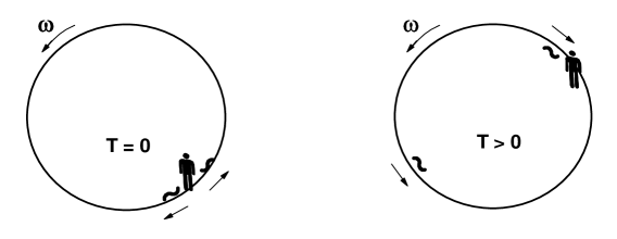
From the ground we see the cw and ccw light pulses having the same speed $c$, the usual value for the speed of light. Note, however, that as the pulses travel around the rim, the rim and the observer fixed to it move as well. Hence, a short time later, as illustrated in the right side of Figure 2, the cw light pulse has returned to the observer, whereas the ccw pulse has yet to do so. A little later (not shown) the ccw pulse will have caught up to the observer.

For the observer, from his perspective on the disk, both light rays travel the same distance, the same number of meters around the circumference. But his experience and his clock readings tell him that the cw pulse took less time to travel the same distance around the circumference than the ccw pulse.

What can he conclude? It appears he can only conclude that, from his point of view, the cw pulse traveled faster than the ccw pulse. Hence, it seems the speed of light as measured on the rotating disk does not always have the same value. It appears different in different directions, and different from that measured on the ground.

This thought experiment makes it plain that any explanation for the Sagnac experiment, from the point of view of the disk reference frame, must account for different arrival times for the cw and ccw light pulses. Analyses based on Doppler shifts or wave length changes are simply not sufficient to explain this. This conclusion accords with GPS[18]^,[19] and other data[26] for the rotating frame of the earth.

APPENDIX B – DERIVING SAGNAC RESULT FROM THE LAB FRAME

Consider Figure 2 of Appendix A with time ($T>0)$ in the right side of the figure when the cw light pulse reaches the disk observer designated as $T_{1}$. Label the time when the ccw pulse reaches the disk observer (not shown) as $T_{2}$. Then lengths traveled as seen from the lab by the ccw light pulse and the observer at $T_{1}$ must sum to equal the circumference, i.e.

$$cT_{1}+\omega RT_{1}=2\pi R\quad\quad\to\quad\quad T_{1}=\frac{2\pi R}{c+\omega R}.$$ (19)

Similarly, at time $T_{2}$

$$cT_{2}=\omega RT_{2}+2\pi R\quad\quad\to\quad\quad T_{2}=\frac{2\pi R}{c-\omega R}.$$ (20)

Hence,

$$\Delta T=T_{2}-T_{1}=\frac{2\omega R}{c^{2}}\frac{2\pi R}{(1-\omega^{2}R^{2}/c^{2})}\approx\frac{4\omega A}{c^{2}}.$$ (21)

As is well known, the standard (physical) clocks on the disk rim run more slowly than the lab clocks by $\sqrt{1-\omega^{2}R^{2}/c^{2}}$, so the observer on the disk must measure an arrival time difference of

$$\Delta t_{phys}=\frac{4\omega A}{c^{2}\sqrt{1-\omega^{2}R^{2}/c^{2}}}.$$ (22)

Steps identical to (15) and (16) yield (1).

APPENDIX C. PHYSICAL VS COORDINATE COMPONENTS

If one has coordinate components, found from generalized coordinate tensor analysis, for some quantity, such as stress or velocity, one needs to be able to translate those into the values measured in experiment. For some inexplicable reason, the method for doing this is not typically taught in general relativity (GR) texts/classes, so it is reviewed here. (Note that often in GR, one seeks invariants like $d\tau$, ds, etc., which are the same in any coordinate system, and in such cases, this issue does not arise. The issue does arise with vectors/tensors, whose coordinate components vary from coordinate system to coordinate system.)

The measured value for a given vector component, unlike the coordinate component, is unique within a given reference frame. In differential geometry (tensor analysis), that measured value is called the “physical component”.

Many tensor analysis texts show how to find physical components from coordinate components[27]. A number of continuum mechanics texts do as well[28]. The only GR text known to the present author that mentions physical components is Misner, Thorne, and Wheeler[29]. Those authors use the procedure to be described below, but do not derive it[30]. The present author has written an introductory article on this, oriented for students, that may be found at the Los Alamos web site[31]. The following is excerpted in part from that article.

The displacement vector $d$x between two points in a 2D Cartesian coordinate system is

$$d{\rm{\bf x}}\,=dX^{1}{\rm{\bf\hat{e}}}_{1}+dX^{2}{\rm{\bf\hat{e}}}_{2}$$ (23)

where the ${\rm{\bf\hat{e}}}_{i}$ are unit basis vectors and dXⁱ are physical components (i.e., the values one would measure with meter sticks). For the same vector $d$x expressed in a different, generalized, coordinate system we have different coordinate components dx${}^{i}\neq$ dXⁱ (dxⁱdo not represent values measured with meter sticks), but a similar expression

$$d{\rm{\bf x}}\,=dx^{1}{\rm{\bf e}}_{1}+dx^{2}{\rm{\bf e}}_{2},$$ (24)

where the generalized basis vectors e_ipoint in the same directions as the corresponding unit basis vectors ${\rm{\bf\hat{e}}}_{i}$, but are not equal to them. Hence, for ${\rm{\bf\hat{e}}}_{i}$, we have

$${\rm{\bf\hat{e}}}_{i}=\frac{{\rm{\bf e}}_{i}}{|{\rm{\bf e}}_{i}|}=\frac{{\rm{\bf e}}_{i}}{\sqrt{{\rm{\bf e}}_{\underline{i}}\cdot{\rm{\bf e}}_{\underline{i}}}}=\frac{{\rm{\bf e}}_{i}}{\sqrt{g_{\underline{i}\underline{i}}}}$$ (25)

where underlining implies no summation.

Substituting (25) into (23) and equating with (24), one obtains

$$dX^{1}=\sqrt{g_{11}}dx^{1}\quad\quad\quad dX^{2}=\sqrt{g_{22}}dx^{2},$$ (26)

which is the relationship between displacement physical (measured with instruments) and coordinate (mathematical value only) components.

Consider a more general case of an arbitrary vector v

$${\rm{\bf v}}=v^{1}{\rm{\bf e}}_{1}+v^{2}{\rm{\bf e}}_{2}=v^{\hat{1}}{\rm{\bf\hat{e}}}_{1}+v^{\hat{2}}{\rm{\bf\hat{e}}}_{2}$$ (27)

where, e₁ and e₂ here do not, in general, have to be orthogonal, e_i and ${\rm{\bf\hat{e}}}_{i}$ point in the same direction for each index $i$, and carets over component indices indicate physical components. Substituting (25) into (27), one readily obtains

$$v^{\hat{i}}=\sqrt{g_{\underline{i}\underline{i}}}v^{i},$$ (28)

which we have shown here to be valid in both orthogonal and non-orthogonal systems.

As a further aid to those readers familiar with anholonomic coordinates (which are associated with non-coordinate basis vectors superimposed on a generalized coordinate grid), we note that physical components are special case anholonomic components where the non-coordinate basis vectors have unit length.

It is important to note that anholonomic components do not transform as true vector components. So one can not simply use physical components in tensor analysis as if they were. Typically, one starts with physical components as input to a problem. These are converted to coordinate components, and the appropriate tensor analysis carried out to get an answer in terms of coordinate components. One then converts these coordinate components into physical components as a last step, in order to compare with values measured with instruments in the real world.

As a basis vector is derived from infinitesimals (derivative at a point), one sees (28) is valid locally in curved, as well as flat, spaces, and can be extrapolated to 4D general relativistic applications. So, very generally, for a 4D vector $v^{\mu}$

$$v^{\hat{i}}=\sqrt{g_{\underline{i}\underline{i}}}v^{i}\quad\quad v^{\hat{0}}=\sqrt{-g_{00}}v^{0},$$ (29)

where Roman sub and superscripts refer solely to spatial components (i.e. $i$ = 1,2,3.)

APPENDIX D – GENERAL PATH DIRECTIONAL TIME DIFFERENCE FOR LIGHT

Relation (8) for the circumferential physical velocity of light on a rotating frame in terms of the circumferential non-rotating frame (lab) velocity generalizes to any such velocity as[32]

$$v_{circum,phys,rot}\,\;=\frac{-r\omega\pm v_{circum,phys,lab}}{\sqrt{1-r^{2}\omega^{2}/c^{2}}}.$$ (30)

We need to find the velocity of light along the path length dl in Figure 3 where the path followed by light is not along a circumferential arc having its center at the axis of rotation. To this end consider dl aligned at an angle $\alpha$ to such a circumferential arc as shown in Figure 3. In order to simplify otherwise unwieldy algebra we will restrict ourselves to first order relations from the outset.

The light travels along dl so we need to find the speed of light along this path in the rotating frame in the positive and negative directions. As before, we label such speeds as $v_{+}$ and $v_{-}$ . According to our first order assumption, we further consider the angle $\alpha$ to have the same value in the lab and rotating frames.

Figure 3: Path of Light Pulses and a Circumferential Element

With the aid of (30), and the understanding implicit in (10) that the velocity of light in the radial direction is the same in the rotating frame as in the lab, we find

$$\begin{array}[]{l}v_{light,circum,lab}=c\cos\alpha\quad\quad\quad\quad\quad v_{light,radial,lab}=c\sin\alpha\\ \\ v_{light,circum,rot}\approx-v\pm c\cos\alpha\quad\quad\quad\quad\quad v_{light,radial,rot}=c\sin\alpha\\ \\ v_{\pm}=v_{light,along\;dl,rot}=\sqrt{(v_{light,circum,rot})^{2}+(v_{light,radial,rot})^{2}}\approx\sqrt{v^{2}+c^{2}\mp 2cv\cos\alpha}\\ \\ \end{array}$$ (31)

Proceeding in parallel fashion to (11) to (14), we find

$$\begin{array}[]{c}d(\Delta t_{phys})=\frac{dl}{v_{+}}-\frac{dl}{v_{-}}\approx\frac{dl}{\sqrt{v^{2}+c^{2}-2cv\cos\alpha}}-\frac{dl}{\sqrt{v^{2}+c^{2}+2cv\cos\alpha}}\\ \\ \approx\frac{dl}{c\sqrt{1-2\textstyle{v\over c}\cos\alpha}}-\frac{dl}{c\sqrt{1+2\textstyle{v\over c}\cos\alpha}}\\ \\ \approx\frac{dl}{c}(1+\textstyle{v\over c}\cos\alpha-1+\textstyle{v\over c}\cos\alpha)\\ \\ =\frac{v}{c^{2}}2dl\cos\alpha\\ \end{array}$$ (32)

We also know

$$dl=\frac{rd\phi}{\cos\alpha}.$$ (33)

Hence

$$d(\Delta t_{phys})\approx\frac{v}{c^{2}}2rd\phi=\frac{2\omega r^{2}d\phi}{c^{2}},$$ (34)

our starting point in Section 4.2.

References

- [1] M. G. Sagnac, “La demonstration de l’existence de l’éther lumineux a travers les mesures d’un interferometre en rotation”, Académie des sciences - Comptes rendus des séances, 157, 708-718 (1913); “Effet tourbillonnaire optique. La circulation de l’éther lumineux dans un interférographe tournant”, Journal de Physique Théorique et Appliquée, Paris, Sociète française de physique, Series 5, Vol 4 (1914), 177-195.
- [2] E.J. Post, ”Sagnac effect,” Rev. Mod. Phys. 39, 475-493 (1967). See eq (1), pg 476.
- [3] C. Møller, C., The Theory of Relativity (Oxford at the Clarendon Press, 1969), pp. 223.
- [4] J. Stachel, ”Einstein and the Rigidly Rotating Disk”, Chapter 1 in Held, General Relativity and Gravitation (Plenum Press, New York, 1980), p. 9; A. Einstein, The Meaning of Relativity (Princeton University Press, 1950), footnote on p. 60.
- [5] B. Mashoon, “Gravitation and nonlocality”, gr-qc/0112058; “The hypothesis of locality and its limitations”, Relativity on a Rotating Frame in series Fundamental Theories of Physics, Editor van der Merwe, A., Kluwer Academic Press (2003).
- [6] E. Minguzzi, “Simultaneity and generalized connections in general relativity”, Class. Quant. Grav. 20, 2443-2456 (2003). gr-qc/0204063. See Section III.
- [7] See ref. [3], p. 223.
- [8] M. Dresden, M., and C.N. Yang, “Phase shift in a rotating neutron or optical interferometer”, Phys. Rev. D. 20(8), 1846-1848 (15 Oct 1979).
- [9] A. Dufour et F. Prunier, “Sur l’observation du phénomène de Sagnac avec une source éclairante non entraînée”, Académie des sciences - Comptes rendus des séances, 204, 1322-1324 (3 May 1937); “Sur un Déplacement de Franges Enregistre sur une Plate-forme en Rotation Uniforme”, Le Journal de Physique et Le Radium, serie VIII, T. III, No 9, 153-161 (Sept 1942).
- [10] F. Selleri, “Noninvariant one-way speed of light and locally equivalent reference frames,” Found. Phys. Lett., 10, 73-83 (1997).
- [11] G. Rizzi, and A. Tartaglia, “Speed of light on rotating platforms”, Found. Phys. 28(11), 1663 (1998).
- [12] S. Bergia, and M. Guidone, “Time on a rotating platform and the one-way speed of light”, Found. Phys. Lett., 11(6), 549-560 (Dec 1998).
- [13] G. Rizzi, and A. Tartaglia, “On local and global measurements of the speed of light on rotating platforms”, Found. Phys. Lett. 12(2), 179-186 (1999).
- [14] G. Rizzi, and M.L. Ruggiero, “Space Geometry of Rotating Platforms: An Operational Approach”, Found. Phys. (in press), gr-qc/0207104.
- [15] R.D. Klauber, “Toward a consistent theory of relativistic rotation”, Relativity on a Rotating Frame in series Fundamental Theories of Physics, Editor van der Merwe, A. (Kluwer Academic Press, 2003).
- [16] R.D. Klauber, “New perspectives on the relatively rotating disk and non-time-orthogonal reference frames”, Found. Phys. Lett. 11(5) 405-443 (1998). qr-qc/0103076
- [17] P. Langevin, “Relativité – Sur l’expérience de Sagnac”, Académie des sciences - Comptes rendus des séances, 205, 304-306 (2 Aug 1937.)
- [18] N. Ashby, “Relativity and the global positioning system”, Phys. Today, May 2002, 41-47. See pg 44.
- [19] N. Ashby, “Relativistic effects in the global positioning system”, 15th Intl. Conf. Gen. Rel. and Grav., Pune, India (Dec 15-21, 1997), available at www.colorado.edu/engineering/GPS/Papers/RelativityinGPS.ps. See pp. 5-7.
- [20] R.D. Klauber, “Comments regarding recent articles on relativistically rotating frames”, Am. Jour. Phys., 67(2), 158-159 (Feb 1999).
- [21] R.D. Klauber, “The speed of light in non-time-orthogonal reference frames and implications for the theory of relativity”, qc-gr/0005121.
- [22] R.D. Klauber, “Non-time-orthogonality and tests of special relativity”, gr-qc/0006023
- [23] R.D. Klauber, “Non-time-orthogonality, gravitational orbits and Thomas precession”, gr-qc/0007018
- [24] R.D. Klauber, “Generalized tensor analysis method and the Wilson and Wilson experiment”, gr-qc/0107035.
- [25] R.D. Klauber, “Analysis of the anomalous Brillet and Hall experimental result”, gr-qc/0210106.
- [26] Y. Saburi, “Observed time discontinuity of clock synchronization in rotating frame of the earth”, J. Rad. Res. Lab., 23 (112), 255-265 (Nov 1976).
- [27] The texts and article listed below are among those that discuss physical vector and tensor components (the values one measures in experiment) and the relationship between them and coordinate components (the mathematical values that depend on the generalized coordinate system being used.) D. Savickas, “Relations between Newtonian Mechanics, general relativity, and quantum mechanics”, Am. J. Phys., 70(8), 798-806 (Aug 2002); I.S. Sokolnikoff, Tensor Analysis (Wiley, 1951) pp. 8, 122-127, 205; G.E. Hay, Vector and Tensor Analysis (Dover, 1953) pp 184-186; A. J. McConnell, Application of Tensor Analysis (Dover, 1947) pp. 303-311; C. E. Pearson, Handbook of Applied Mathematics (Van Nostrand Reinhold, 1983, 2nd ed.), pp. 214-216; M. R. Spiegel, Schaum’s Outline of Vector Analysis (Schaum), pg. 172; R. C. Wrede, Introduction to Vector and Tensor Analysis (Dover, 1972), pp. 234-235.
- [28] L.E. Malvern, Introduction to the Mechanics of a Continuous Medium (Prentice-Hall, Englewood Cliffs, New Jersey, 1969). See Appendix I, Sec. 5, pp. 606-613. Y.C. Fung, Foundations of Solid Mechanics (Prentice-Hall, Inc., Englewood Cliffs, NJ, 1965). See pp. 52-53 and 111-115. A.C. Eringen, Nonlinear Theory of Continuous Media (McGraw-Hill, NY, 1962), pp. 437-439. T.J. Chung, Continuum Mechanics (Prentice Hall, Englewood Cliffs, NJ, 1988), pp. 40-53, 246-251.
- [29] Misner, C.W., Thorne, K.S., and Wheeler, J.A., Gravitation (Freeman, New York, 1973).
- [30] Physical components are introduced in ref. [29] on pg. 37, and used in many places throughout the text, though surprisingly, the relation between physical and coordinate components is not derived. It is used, however. See, for example, physical velocity components found in equation (31.5) on pg. 821.
- [31] Klauber, R.D., “Physical components, coordinate components, and the speed of light”, gr-qc/0105071;
- [32] Ref [15], pp. 424-425.