Optimal Strategies for Sinusoidal Signal Detection

Abstract

We derive and study optimal and nearly-optimal strategies for the detection of sinusoidal signals hidden in additive (Gaussian and non-Gaussian) noise. Such strategies are an essential part of algorithms for the detection of the gravitational Continuous Wave (CW) signals produced by pulsars. Optimal strategies are derived for the case where the signal phase is not known and the product of the signal frequency and the observation time is non-integral.

I INTRODUCTION

A key problem in data analysis is to detect sinusoidal signals in noise. Such signals are often called “lines” or “peaks” because in the Fourier domain (frequency space) they appear as spikes (line-like features) or sharp narrow peaks in the energy spectrum of the signal. When the signal is large compared to the noise, such signals are easy to identify. When they are weak, the identification becomes more difficult.

The work in this paper was motivated by the development of algorithms to search for Continuous Wave (CW) signals in the new generation of interferometric gravitational-wave detectors which are either under construction science92 ; physicstoday ; virgo ; geo600 ; tama300 or planned plannedinstruments . These signals are produced by rapidly spinning neutron stars (pulsars).

To search for new (previously undetected) pulsars requires a search over possible sky positions, frequencies, and pulsar spin-down parameters. The parameter space is very large and these searches are computationally very intensive. Moreover the searches will be looking for signals that are (statistically) at the lower limit of detection sensitivity 300years .

A brute-force approach (optimally filtering for all possible source parameters) requires unrealistic computational resources (Petaflops), so more sophisticated hierarchical approaches have been proposed. When the parameter space is very large, these approaches retain much or all of the sensitivity of the brute-force approach but require less computational resources. This is possible because, in the brute-force approach, the number of grid points in parameter space is so large that the detection threshold must be set very high to avoid false alarms and enable confident detection. A hierarchical search visits fewer points in parameter space: it ignores those below the (high) threshold that one must set in order to gain the necessary detection confidence while examining a large parameter space. In other words a hierarchical search method does not “waste” precious computational cycles examining regions in parameters space where, even if a signal were present, it would not be detected confidently enough.

The hierarchical search techniques bccs ; schutz2 ; schutzpapa ; bradycreighton all involve a second (so-called incoherent) stage. This stage is called “incoherent” because it uses spectral rather than amplitude data. If one neglects polarization, in all of the proposed approaches a putative signal at the second stage would (effectively) appear in a spectrum as a sinusoidal signal at fixed frequency and phase. The third stage of the search works only on the regions in parameter space where significant spectral lines were identified in the second stage.

Our paper addresses the problem of identifying these candidates, that is “registering” candidate sinusoidal signals. The analysis makes use of the Neyman-Pearson criteria to identify the “best” statistic to use for such identification. In some cases, the best statistic depends upon the expected amplitude of the signal, which is unknown. In these cases, we have used locally-optimal methods to identify the best statistic in the weak-signal limit.

The analysis is complicated by several factors:

• The signal frequency and phase are not known in advance.

• The signal frequency may not lie at an integer multiple of the Rayleigh frequency $T^{-1}$. A signal of this type does not make an integer number of cycles during the observation time $T$. We call such frequencies, and the corresponding signal, “unresolved”.

• The signal frequency must be identified with resolution less than $\pm(2T)^{-1}$, i.e., to within the nearest frequency bin.

• The method must handle non-Gaussian noise in an optimal manner.

The analysis presented here addresses all of these concerns.

II PROBLEM DESCRIPTION AND OPTIMAL STATISTICS

The basic problem that we consider is the following. We are given $N$ samples of a time-domain data stream, sampled at discrete times $t=t_{j}=j\Delta t$. We denote this data by $y_{j}$ for $j=0,1,\cdots,N-1$. The total observation time is $T=N\Delta t$. The question that we want to answer is, does the data stream $y_{j}$ contain a sinusoidal signal

$$y_{j}=\epsilon{2\over N}\cos(2\pi ft_{j}-\phi)$$ (1)

of constant amplitude and frequency? To address this question, we make use of the theory of optimal signal detection. It is convenient to recast the problem in the Fourier domain. Denote the Discrete Fourier Transform (DFT) of the data by $x_{k}$:

$$x_{k}=\sum_{j=0}^{N-1}y_{j}{\rm e}^{2\pi ijk/N},\qquad\text{for\ }{\scriptstyle k=-N/2+1,\cdots,N/2}.$$ (2)

Since this transformation is invertible, any question or statement about the $y$’s can also be stated in terms of the $x$’s, hence we will often use the term “data” to refer to the $x$’s rather than to the $y$’s. Here, and elsewhere, the symbols $x$ and $y$ without indices refer to the collective ensemble of all the data. For convenience we will assume that $N$ is a power of two. The index $k$ will often be referred to as a “frequency bin”. The frequencies that these bins correspond to,

$$f_{k}={k\over N\Delta t}={k\over T}$$ (3)

are called “resolved frequencies” for reasons that will become clear later.

In what follows, we will assume that the data $y$ is real. In this case, $x_{k}=x_{-k}^{*}$ where ^∗ denotes complex-conjugate, and both $x_{0}$ and $x_{N/2}$ are real. The data set $y$ is then exactly equivalent to the set of $x_{k}$ for $k=0,\cdots,N/2$. To simplify the mathematics, we will assume that the average value of the $y$’s vanishes (i.e., that the DC or average value has been removed from the data) so that $x_{0}=0$. We will also assume that there is no energy at the Nyquist frequency $f_{N/2}$ (which in a real experiment would be enforced by appropriate anti-aliasing filters) so that $x_{N/2}=0$. Then, the data set $y$ is exactly equivalent to the set $x_{k}$ for $k=1,\cdots,N/2-1$.

We use the notation $p(x|\epsilon)$ to denote the probability distribution function (pdf) of the data, in the presence of a signal whose amplitude is $\epsilon$. For example,

• if the (real and imaginary parts of the) noise in each frequency bin is independent and Gaussian with vanishing mean and unit variance, and the signal is a sinusoid of known phase at resolved frequency $f_{\ell}$ given by $y_{j}=\epsilon{2\over N}\cos(2\pi f_{\ell}t_{j}-\phi)$, then

  $$p(x|\epsilon)={1\over 2\pi}{\rm e}^{-{1\over 2}|x_{\ell}-\epsilon{\rm e}^{i\phi}|^{2}}\mathop{\prod_{k=1}^{N/2-1}}_{k\neq\ell}{1\over 2\pi}{\rm e}^{-{1\over 2}|x_{k}|^{2}}.$$

  Note that since $\ell$ is an integer, and $\epsilon$ is real, the signal only affects the $\ell$’th frequency bin.

• if the assumptions are the same as above, but the phase of the signal is unknown and uniformly distributed over the range $\phi\in[0,2\pi)$, then

  $$p(x|\epsilon)={1\over 2\pi}\int_{0}^{2\pi}d\phi{1\over 2\pi}{\rm e}^{-{1\over 2}|x_{\ell}-\epsilon{\rm e}^{i\phi}|^{2}}\mathop{\prod_{k=1}^{N/2-1}}_{k\neq\ell}{1\over 2\pi}{\rm e}^{-{1\over 2}|x_{k}|^{2}}.$$

Somewhat later, we will relax these assumptions, and give more general forms for $p(x|\epsilon)$ where

• the signal frequency is not a resolved frequency,

• the noise is not white, and

• the noise is not Gaussian.

Note that the integration measure for $p(x|\epsilon)$ is

$$\int dx\equiv\prod_{k=1}^{N/2-1}\int_{-\infty}^{\infty}d\Re x_{k}\int_{-\infty}^{\infty}d\Im x_{k},$$

where $\Re$ and $\Im$ denote the real and imaginary parts.

The problem that we wish to solve is well-known in the theory of signal detection. The space of possible measurements $x_{k}$ for $k=1,...,N/2-1$ is $\mathbf{R}^{N-2}$. Our goal is to divide this space of possible measurements into two disjoint regions $H_{0}$ and $H_{1}$, whose union is all of $\mathbf{R}^{N-2}$. If the observed data lies in $H_{0}$ (the “null-hypothesis region”) we will conclude that no signal was present in the data. If the data lies in $H_{1}$, we will conclude that a signal was present. The problem we need to solve is this: what is the best choice of $H_{0}$ and $H_{1}$?

The solution we chose is the Neyman-Pearson criterion: the best choice is the one that gives the lowest false dismissal probability for a given false alarm probability. The false alarm probability $\alpha$ is the probability that a signal is detected when none is present:

$$\alpha=\int_{x\in H_{1}}dx\;p(x|0),$$ (4)

and the false dismissal probability $\beta(\epsilon)$ is the probability that a signal of amplitude $\epsilon$ is not found:

$$\beta(\epsilon)=\int_{x\in H_{0}}dx\;p(x|\epsilon)$$ (5)

The Neyman-Pearson criteria leads immediately to the following rule to partition the space of possible measurements into $H_{0}$ and $H_{1}$. Define the likelihood function on the space of possible measurements by

$$\Lambda(x)={p(x|\epsilon)\over p(x|0)}$$

and consider the surface $\Lambda(x)=\Lambda_{0}=\text{constant}$. The Neyman-Pearson criteria leads to the following choice: take $H_{0}$ to be the region inside this surface, and $H_{1}$ to be the region outside this surface. The value of $\Lambda_{0}$ that defines the surface determines the false alarm and false dismissal probabilities.

In this paper, we will use the Neyman-Pearson criteria to define an “optimal statistic” which we will denote $\tau(x)$. This is any function of the observed data $x$ whose level surfaces are the same as the level surfaces of $\Lambda(x)$. If the statistic is greater than some threshold $\cal T$ then we conclude that a signal is present, and if the statistic is less than the threshold $\cal T$ we conclude that no signal was present. The false alarm and false dismissal probabilities are functions of this threshold $\cal T$: as $\cal T$ is increased the false alarm probability gets smaller, and the false dismissal probability gets larger. In general this optimal statistic is a function of the signal amplitude $\epsilon$. However we will see that for the pulsar detection problem, where $\epsilon$ is small, the optimal statistic is effectively $\epsilon$-independent.

III A WORKED EXAMPLE

To help make these ideas concrete, we give a complete worked example, demonstrating these ideas for the second pdf described above: a signal of unknown phase at a resolved frequency $f_{\ell}$. The pdf is

$$p(x|\epsilon)={1\over 2\pi}\int_{0}^{2\pi}d\phi{1\over 2\pi}{\rm e}^{-{1\over 2}|x_{\ell}-\epsilon{\rm e}^{i\phi}|^{2}}\mathop{\prod_{k=1}^{N/2-1}}_{k\neq\ell}{1\over 2\pi}{\rm e}^{-{1\over 2}|x_{k}|^{2}}.$$ (6)

Before continuing, it is convenient to express this in closed form. Writing the complex data sample $x_{\ell}=|x_{\ell}|\exp(i\psi_{\ell})$ in terms of its modulus $|x_{\ell}|$ and phase $\psi_{\ell}$, one has

$${1\over 2\pi}\int_{0}^{2\pi}d\phi{1\over 2\pi}{\rm e}^{-{1\over 2}|x_{\ell}-\epsilon{\rm e}^{i\phi}|^{2}}$$

$$= {1\over 2\pi}\int_{0}^{2\pi}d\phi{1\over 2\pi}{\rm e}^{-{1\over 2}\left(|x_{\ell}|^{2}+\epsilon^{2}-2\epsilon\Re(x_{\ell}^{*}{\rm e}^{i\phi})\right)}$$

$$= {1\over 2\pi}{\rm e}^{-{1\over 2}(|x_{\ell}|^{2}+\epsilon^{2})}{1\over 2\pi}\int_{0}^{2\pi}d\phi\;{\rm e}^{\epsilon|x_{\ell}|\cos(\phi-\psi_{\ell})}$$

$$= {1\over 2\pi}{\rm e}^{-{1\over 2}(|x_{\ell}|^{2}+\epsilon^{2})}I_{0}(\epsilon|x_{\ell}|).$$

The final integral has been expressed in terms of a modified Bessel function $I_{0}(r)$ of the first kind

$$I_{0}(r)={1\over\pi}\int_{0}^{\pi}d\theta\;{\rm e}^{r\cos\theta}.$$

Thus we obtain a closed form for the pdf (6)

$$p(x|\epsilon)={\rm e}^{-{1\over 2}\epsilon^{2}}I_{0}(\epsilon|x_{\ell}|)\prod_{k=1}^{N/2-1}{1\over 2\pi}{\rm e}^{-{1\over 2}|x_{k}|^{2}}.$$ (7)

The likelihood function is now easily found:

$$\Lambda(x)={p(x|\epsilon)\over p(x|0)}={\rm e}^{-{1\over 2}\epsilon^{2}}I_{0}(\epsilon|x_{\ell}|).$$ (8)

While in a general situation, the likelihood function depends upon all the different variables, in this particular situation it only depends upon $|x_{\ell}|$.

We defined an optimal statistic $\tau$ to be any function whose level surfaces are the same as the level surfaces of the likelihood function $\Lambda(x)$. In this simple situation, the likelihood function $\Lambda(x)=\Lambda(x_{1},\cdots,x_{N/2-1})$ only depends upon the modulus $|x_{\ell}|$ of the amplitude in a single (the $\ell$’th) Fourier bin. Since it is a monotonically increasing function of $|x_{\ell}|$, we can choose as an optimal statistic any monotonic function of $|x_{\ell}|$, for example $|x_{\ell}|$ or $|x_{\ell}|^{2}$. For historical and later convenience, let us choose as our optimal statistic the function $\tau=|x_{\ell}|^{2}$. This is the power in the $\ell$’th bin. The mean value of this statistic, the power in the $\ell$’th bin, is

$$\int dx\;\tau\;p(x|\epsilon)=\int dx\;|x_{\ell}|^{2}p(x|\epsilon)=2+\epsilon^{2}.$$ (9)

In the absence of a signal ($\epsilon=0$) both the real and imaginary parts of $x_{\ell}$ contribute unity.

To complete the analysis of this example, we need to calculate the false alarm and false dismissal probabilities. We will define, for a given value of threshold $\cal T$, the regions $H_{0}$ and $H_{1}$ by:

$$H_{0} = \left\{(x_{1},\cdots,x_{N/2-1})\;\text{such that}\;\tau=|x_{\ell}|^{2}\leq\cal T\right\},\text{ and}$$

$$H_{1} = \left\{(x_{1},\cdots,x_{N/2-1})\;\text{such that}\;\tau=|x_{\ell}|^{2}>\cal T\right\}.$$

Thus our choice of statistic gives a decision rule which has a simple physical interpretation. If the power in bin $\ell$ is greater than $\cal T$, we conclude that a signal was present. If not, we conclude that no signal was present.

The false alarm probability (4) is easy to calculate. It is given by the following function of threshold $\cal T$.

$$\alpha(\cal T) = \int_{x\in H_{1}}dx\;p(x|0)$$ (10)

$$= \int_{|x_{\ell}|^{2}>\cal T}dx\;p(x|0)$$ (11)

$$= \int_{|x_{\ell}|^{2}>\cal T}dx\prod_{k=1}^{N/2-1}{1\over 2\pi}{\rm e}^{-{1\over 2}|x_{k}|^{2}}$$ (12)

$$= \mathop{\int d\Re x_{\ell}\int d\Im x_{\ell}}_{|x_{\ell}|^{2}>\cal T}{1\over 2\pi}{\rm e}^{-{1\over 2}|x_{\ell}|^{2}}$$ (13)

$$= \int_{0}^{2\pi}d\psi_{\ell}\int_{|x_{\ell}|=\sqrt{\cal T}}^{\infty}|x_{\ell}|d|x_{\ell}|{1\over 2\pi}{\rm e}^{-{1\over 2}|x_{\ell}|^{2}}$$ (14)

$$= \int_{{\cal T}/2}^{\infty}d\left({1\over 2}{|x_{\ell}|^{2}}\right){\rm e}^{-{1\over 2}{|x_{\ell}|^{2}}}$$ (15)

$$= {\rm e}^{-{\cal T}/2}$$ (16)

In this calculation, the transition from the 3rd to the 4th line is trivial because we integrate over the all the coordinates except for $x_{\ell}$. In going from the 4th to the 5th line, we have changed variables from real and imaginary parts, to polar coordinates.

The false dismissal probability (5), which depends both upon the signal amplitude $\epsilon$ and upon the value $\cal T$ of the decision statistic threshold, is obtained with a similar calculation.

$$\beta(\cal T) = \int_{x\in H_{0}}dx\;p(x|\epsilon)$$ (17)

$$= \int_{|x_{\ell}|^{2}\leq\cal T}dx\;p(x|\epsilon)$$ (18)

$$= {\rm e}^{-{1\over 2}\epsilon^{2}}\int_{0}^{\sqrt{\cal T}}|x_{\ell}|d|x_{\ell}|{\rm e}^{-{1\over 2}|x_{\ell}|^{2}}I_{0}(\epsilon|x_{\ell}|)$$ (19)

$$= {\rm e}^{-{1\over 2}\epsilon^{2}}\int_{0}^{{\cal T}/2}du\;{\rm e}^{-u}I_{0}(\epsilon\sqrt{2u})$$ (20)

This final integral can not be evaluated in closed form. However it is easy to check that the limit $\beta(\infty)=1$: if the threshold is set very large, then the false dismissal probability is unity. In a moment, we will study the behavior of $\beta$ in the weak-signal limit as $\epsilon\to 0$. However, before this, it is instructive to study the false-alarm versus false-dismissal curves for this statistic.

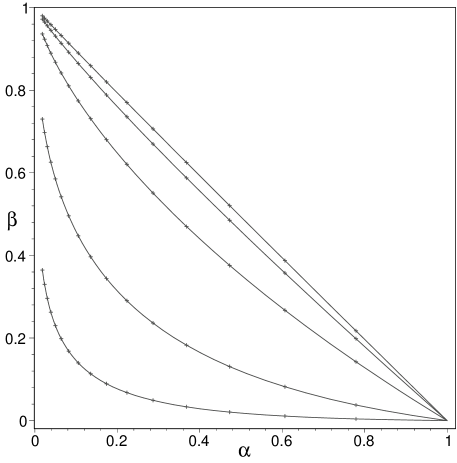
Figure 1: The false dismissal probability $\beta({\cal T})$ as a function of the false alarm probability $\alpha({\cal T})$ for different values of the signal amplitude $\epsilon$. The top curve has $\epsilon=0.2$. Moving down, the remaining curves have $\epsilon=0.5,1.0,2.0,3.0$. Along each curve, the threshold ${\cal T}$ varies from 0 to 8. In the bottom right of the graph, ${\cal T}=0$. The crosses mark the points where ${\cal T}=1/2,1,3/2,\cdots,8$. For example, with a threshold ${\cal T}=5.5$, if the signal amplitude is $\epsilon=3$, then the false alarm probability is $\alpha\approx 6.4\%$ and the false dismissal probability is $\beta\approx 20\%$.

The false alarm and false dismissal curves for this optimal detection statistic are illustrated in Fig. 1. Plotting $\beta$ as a function of $\alpha$ provides a way of describing the optimal statistic which is completely independent of the actual choice of the statistic. However, the relationship between the threshold $\cal T$ and the false alarm and false dismissal probability does depend upon the choice of optimal statistic. Because this statistic has been chosen by the Neyman-Pearson criterion, any other detection statistic that we choose will have poorer performance. Thus, for a given signal amplitude $\epsilon$, and for a given false alarm probability $\alpha$, any other detection statistic will have a larger false dismissal probability $\beta$: it will lie above the illustrated curves.

Our primary interest is in very weak signals. For the pulsar detection problem, we will have $\epsilon\approx 0.2$, and will be operating on the threshold of detection where $\alpha+\beta$ is only slightly smaller than unity. For such weak signals, it is useful to define the quantity

$$\gamma({\cal T})=1-\alpha({\cal T})-\beta({\cal T}).$$ (21)

This may be considered either as a function of the threshold $\cal T$ or as a function of the false alarm probability $\alpha({\cal T})$. This quantity $\gamma$ is the difference between the detection probability when a signal is present, $1-\beta$, and the false alarm probability $\alpha$. For example, for a very weak signal, the threshold might be set for a false alarm probability of $\alpha=15\%$. The false dismissal probability for this weak signal might be $\beta=84\%$. Thus, if no signal is present, the threshold will be exceeded $\alpha=15\%$ of the time. If a signal is present, the threshold will be exceeded $1-\beta=16\%$ of the time. Roughly speaking, the difference between these, $\gamma=1-\alpha-\beta=1\%$, is the probability of the threshold being exceeded because the signal was present, rather than because of the detector noise. These weak-signal-limit curves are shown in Fig. 2.

In the small-$\epsilon$ (weak signal) limit, it is easy to obtain an approximate closed-form for $\beta$. By substituting the power series representation of the Bessel function,

$$I_{0}(x)=1+{x^{2}\over 4}+{x^{4}\over 64}+{x^{6}\over 2304}+\cdots$$

into Eqn. (17) and integrating term-by-term, one obtains

$$\gamma=1-\alpha-\beta=$$ (22)

$${\epsilon^{2}\over 4}{\cal T}{\rm e}^{-{\cal T}/2}\left[1+{\epsilon^{2}\over 16}({\cal T}-4)+{\epsilon^{4}\over 576}({\cal T}^{2}-12{\cal T}+24)+\cdots\right]$$

$$=-{1\over 2}\epsilon^{2}\alpha\ln\alpha\left[1-{\epsilon^{2}\over 8}(2+\ln\alpha)\right.$$

$$\left.\hskip 60.0pt+{\epsilon^{4}\over 144}\left(6+6\ln\alpha+(\ln\alpha)^{2}\right)+\cdots\right].$$

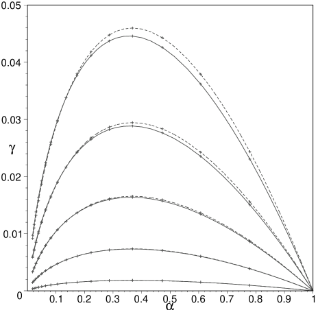
Even at the lowest order in $\epsilon$ (the first term in square brackets) this is a very good approximation, as shown by the dashed curves in Fig. 2. At the next order (the first two terms in square brackets) the approximation is indistinguishable from the exact result in Fig. 2 – the solid curves. This simplifies matters enormously. Although the statistics of the optimal detection strategy depends upon the signal amplitude $\epsilon$, for small $\epsilon$, this dependence is simple enough to be analytically approximated.

Figure 2: Solid curves: detection probability $\gamma=1-\alpha-\beta$ as a function of the false alarm probability $\alpha$ for different values of the signal amplitude $\epsilon=0.1,\cdots,0.5$ (moving up from the bottom curve). The crosses mark different values of the threshold in the same way as for Fig. 1. Dashed curves: the $O(\epsilon^{2})$ approximation is $\gamma=\epsilon^{2}{\cal T}\exp(-{\cal T}/2)/4=-\epsilon^{2}\alpha\ln\alpha/2$. The $O(\epsilon^{4})$ approximation to $\gamma$ is not shown because on this graph it is indistinguishable from the exact result (the solid curves).

The detection probability plays a key role in the significance of an observation. A hierarchical pulsar search hunts for peaks in the spectra coming from a set of $n$ sequential time series. For example, suppose each time series of length $N$ is one day long. Three months of such data would correspond to $n=120$. What choice of false alarm probability $\alpha$ (or equivalently, of detection threshold $\cal T$) is optimal?

This question is easily answered. One might guess that the best operating point is where the detection probability $\gamma=1-\alpha-\beta$ is maximized: in the weak signal case this is at a threshold of ${\cal T}=2$ corresponding to a false alarm probability $\alpha=1/e\approx 36.78\%$. However this is not correct. In the absence of signal, each of the $n$ data sets is independent. The probability of detecting peaks in $p$ of the $n$ data sets is the same as the probability that a coin will come up heads $p$ times in $n$ flips (if the probability of “heads” is the false alarm probability $\alpha$). This is given by the binomial distribution:

$$\text{probability of p peaks}=\left(\begin{array}[]{c}n\\ p\end{array}\right)\alpha^{p}(1-\alpha)^{n-p}.$$

Thus, in the absence of a signal, the mean number of peaks is $\alpha n$, and its variance is $\sigma^{2}=\alpha(1-\alpha)n$. In the presence of a signal, the mean number of peaks registered is $(1-\beta)n$. A good way to choose a false alarm probability (or threshold) is to maximize the significance $s$. This is

$$s = {\langle\text{\# peaks}\rangle_{\rm signal}-\langle\text{\# peaks}\rangle_{\rm no\ signal}\over\sigma}$$ (23)

$$= {(1-\beta)n-\alpha n\over\sqrt{\alpha(1-\alpha)n}}$$

$$= {1-\alpha-\beta\over\sqrt{\alpha(1-\alpha)}}\sqrt{n}$$

$$= {\gamma\over\sqrt{\alpha(1-\alpha)}}\sqrt{n}$$

The significance is easily calculated as a function of either $\alpha$ or $\cal T$. In the weak-signal limit, it is

$${s\over\sqrt{n}}={\epsilon^{2}\over 4}{{\cal T}\over\sqrt{{\rm e}^{{\cal T}/2}-1}}=-{\epsilon^{2}\over 2}\sqrt{\alpha\over 1-\alpha}\ln\alpha$$

The significance as a function of either ${\cal T}$ or $\alpha$ has a maximum at the threshold value ${\cal T}\approx 3.18721$ corresponding to a false alarm probability of $\alpha\approx 20.3188\%$. The significance at this threshold/false alarm probability is $s\approx 0.402371\epsilon^{2}\sqrt{n}$. Note that this exhibits the expected $\sqrt{n}$ scaling in the number $n$ of spetra analyzed. We have numerically verified that this is the optimal statistic.

IV EXAMPLE: LOCAL PEAK DETECTION – A NON-OPTIMAL STRATEGY

Section III found and analyzed the optimal (i.e. Neyman-Pearson) peak detection strategy. In this Section, we carry out an identical analysis of a different (hence non-optimal) strategy. The main purpose is to illustrate a side-by-side comparison of different detection statistics.

We will assume that the signal and noise satisfy the same assumptions as in Section III, given by Eqn. (7). There, we showed that the optimal detection strategy was to threshold on the power $\tau=|x_{\ell}|^{2}$ in the $\ell$’th bin. Here, we adopt a different detection strategy. We will say that a peak has been detected if and only if the power $|x_{\ell}|^{2}$ in the $\ell$’th bin exceeds the threshold $\cal T$ and is greater than the power in either of the neighboring frequency bins. This strategy looks for “local peaks” that exceed the threshold.

For this peak detection strategy, the detection region $H_{1}$ is defined by

$$H_{1} = \Big{\{}(x_{1},\cdots,x_{N/2-1})\;\text{such that}$$

$$|x_{\ell}|^{2}>{\cal T}\text{ and }|x_{\ell}|^{2}>|x_{\ell-1}|^{2}\text{ and }|x_{\ell}|^{2}>|x_{\ell+1}|^{2}\Big{\}}.$$

In other words, the peak detection strategy is to register a peak if the observed data set lies in $H_{1}$. The null-hypothesis or no-signal region $H_{0}$ is the set complement $H_{0}=\mathbf{R}^{N-2}-H_{1}$: all points not lying in $H_{1}$.

To compare this strategy to the optimal one found in Section III, we calculate the false-alarm and false-detection curves as before, and compare them with the optimal strategy. The false alarm probability is

$$\alpha(\cal T) = \int_{x\in H_{1}}dx\;p(x|0)$$

$$= \mathop{\int{dx_{\ell-1}\over 2\pi}\int{dx_{\ell}\over 2\pi}\int{dx_{\ell+1}\over 2\pi}}_{\begin{array}[]{c}|x_{\ell}|^{2}>{\cal T}\\ |x_{\ell}|^{2}>|x_{\ell-1}|^{2}\\ |x_{\ell}|^{2}>|x_{\ell+1}|^{2}\end{array}}{\rm e}^{-{1\over 2}(|x_{\ell-1}|^{2}+|x_{\ell}|^{2}+|x_{\ell+1}|^{2})}$$

In these expressions, $\int dx_{k}$ denotes $\int_{-\infty}^{\infty}d\Re x_{k}\int_{-\infty}^{\infty}d\Im x_{k}$. Putting each of the three integrals into polar coordinates immediately yields

$$\alpha(\cal T) = {1\over 2}\int_{\cal T}^{\infty}d|x_{\ell}|^{2}\;{\rm e}^{-|x_{\ell}|^{2}/2}\left[{1\over 2}\int_{0}^{|x_{\ell}|^{2}}d|x_{\ell-1}|^{2}\;{\rm e}^{-|x_{\ell-1}|^{2}/2}\right]^{2}$$ (25)

$$= {1\over 2}\int_{\cal T}^{\infty}d|x_{\ell}|^{2}\;{\rm e}^{-|x_{\ell}|^{2}/2}\left[\left.-{\rm e}^{-u/2}\right|_{u=0}^{u=|x_{\ell}|^{2}}\right]^{2}$$

$$= {1\over 2}\int_{\cal T}^{\infty}d|x_{\ell}|^{2}\;{\rm e}^{-|x_{\ell}|^{2}/2}\left[1-{\rm e}^{-|x_{\ell}|^{2}/2}\right]^{2}$$

$$= \int_{{\cal T}/2}^{\infty}du\;{\rm e}^{-u}\left[1-{\rm e}^{-u}\right]^{2}$$

$$= {1\over 3}{\rm e}^{-{3\over 2}{\cal T}}-{\rm e}^{-{\cal T}}+{\rm e}^{-{1\over 2}{\cal T}}$$

The quantity in square brackets that appears in the intermediate steps of this calculation is simply the probability that bins $\ell\pm 1$ contain less power than the $\ell$’th bin. This is one minus the false alarm probability (10) of the optimal test.

As with the optimal test, the false alarm probability $\alpha({\cal T})$ vanishes at large threshold $\cal T\to\infty$. However, unlike the optimal test, the false alarm probability at zero threshold is not unity: $\alpha({\cal T}=0)=1/3$. This is because, even if the threshold vanishes, to register as a peak the $\ell$’th bin must contain more power than both adjacent bins. When no signal is present, this only happens $1/3$ of the time.

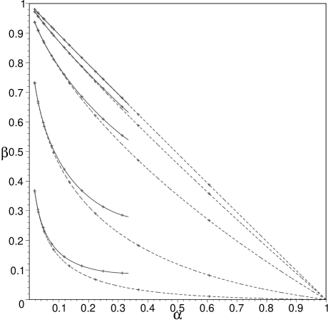
Figure 3: Solid curves: false-dismissal $\beta$ versus false-alarm $\alpha$ for the non-optimal detection strategy of this Section. Moving down from the top, the curves correspond to signal strengths $\epsilon=0.2,0.5,1,2,3$. Notice that the false alarm probability $\alpha$ is less than $1/3$ for any value of the threshold $\cal T$. For comparison, the dashed curves show the optimal strategy of the previous Section. Notice that the optimal strategy always yields a lower false dismissal probability for a given false alarm probability. The crosses mark threshold values ${\cal T}=1,2,\cdots,8$ increasing to the left along each curve.

The false dismissal probability for this non-optimal peak detection strategy can be calculated with the same methods as above. One finds

$$\beta({\cal T})=\int_{x\in H_{0}}dx\;p(x|\epsilon)$$

$$= 1-\int_{x\in H_{1}}dx\;p(x|\epsilon)$$

$$= 1-{1\over 2}\int_{\cal T}^{\infty}d|x_{\ell}|^{2}\;{\rm e}^{-{1\over 2}\left(|x_{\ell}|^{2}+\epsilon^{2}\right)}I_{0}(\epsilon|x_{\ell}|)\left[1-{\rm e}^{-|x_{\ell}|^{2}/2}\right]^{2}$$

$$= 1-{\rm e}^{-{1\over 2}\epsilon^{2}}\int_{{\cal T}/2}^{\infty}du\;I_{0}(\epsilon\sqrt{2u})\;{\rm e}^{-u}\left[1-{\rm e}^{-u}\right]^{2}$$

$$= {\rm e}^{-{1\over 4}\epsilon^{2}}-{\scriptstyle{1\over 3}}{\rm e}^{-{1\over 3}\epsilon^{2}}+{\rm e}^{-{1\over 2}\epsilon^{2}}\int_{0}^{{\cal T}/2}du\;I_{0}(\epsilon\sqrt{2u})\;{\rm e}^{-u}\left[1-{\rm e}^{-u}\right]^{2}$$

As for the optimal statistic, this false dismissal probability approaches one at large threshold ${\cal T}\to\infty$. However, unlike the optimal test, it does not vanish at zero threshold. Setting ${\cal T}=0$ in (IV) on finds that

$$\beta({\cal T}=0)={\rm e}^{-\epsilon^{2}/4}-{1\over 3}{\rm e}^{-\epsilon^{2}/3}.$$

If the signal amplitude is small $\epsilon\to 0$ then $\beta({\cal T}=0)\to 2/3$. There is a $2/3$ probability of missing a small signal at zero threshold, because one of the two neighboring frequency bins might contain more power than bin $\ell$.

A set of false alarm/false dismissal curves for this non-optimal statistic are shown in Fig. 3, along with the same curves for the optimal statistic. Note that for a given signal strength and false alarm probability, the false dismissal probability is always lower for the Neyman-Pearson test. Also notice that a given value of the threshold for one test statistic does not yield the same false alarm probability as the same threshold value for the other statistic. As the false alarm probability decreases, the two statistics have a performance (false dismissal probability) that becomes increasingly similar. This is because at increasing values of the threshold ${\cal T}$, fewer and fewer peaks are rejected because the neighboring peaks are larger.

Figure 4: These graphs are a comparison of two different peak-finding methods, in the weak signal limit (small $\epsilon$). The dashed curves correspond to the optimal (Neyman-Pearson) test: thresholding on the signal power. The solid curves correspond to the local peak test described in this Section. The bottom graph shows the detection probability $\gamma/\epsilon^{2}=(1-\alpha-\beta)/\epsilon^{2}$ as a function of false alarm probability $\alpha$. The top graph shows the significance $\gamma\over\epsilon^{2}\sqrt{\alpha(1-\alpha)}$. Table 1 compares the properties of these curves.

In the small-signal limit $\epsilon\to 0$, one can use the series expansion of the Bessel function to obtain analytic expressions for the false alarm probability $\beta$. The signal detection probability is

$$\gamma=1-\alpha-\beta$$

$$= {\epsilon^{2}{\rm e}^{-3{\cal T}/2}\over 4}\left[{\cal T}\left({\rm e}^{{\cal T}}-{\rm e}^{{\cal T}/2}+{1\over 3}\right)+\;{\rm e}^{{\cal T}/2}-{4\over 9}\right]+O(\epsilon^{4})$$

$$= {\epsilon^{2}\over 4}\left[\alpha{\cal T}+{\rm e}^{-{\cal T}}-{4\over 9}{\rm e}^{-3{\cal T}/2}\right]+O(\epsilon^{4}).$$

This signal detection probability can’t be expressed in analytic form entirely in terms of $\alpha$ given by (25). However we can plot it and compare with the identical curve for the optimal strategy. This is shown in Fig. 4, which also shows the significance as a function of the false alarm probability. The comparison is shown in Table 1.

	Optimal Test	Local Peak Test
Maximum of $1-\alpha-\beta$ =	$0.1839\;\epsilon^{2}$	$0.1529\;\epsilon^{2}$
is at threshold value $\cal T$ =	$2.0$	$2.0$
and false alarm prob $\alpha$ =	36.79%	24.91%
Maximum of ${1-\alpha-\beta\over\sqrt{\alpha(1-\alpha)}}$ =	$0.4024\;\epsilon^{2}$	$0.3806\;\epsilon^{2}$
is at threshold value $\cal T$ =	$3.187$	$3.567$
and false alarm prob $\alpha$ =	$20.32\%$	$14.14\%$

Table 1: A comparison of the optimal Neyman-Pearson detection strategy, and the sub-optimal local peak detection method, in the weak-signal limit. Most of these values can be read off Fig. 4. The top half of the table gives information about the maximum of $\gamma=1-\alpha-\beta$, such as the value of the threshold at the maximum. The bottom half of the table gives the same information for the maximum of ${1-\alpha-\beta\over\sqrt{\alpha(1-\alpha)}}$.

The primary purpose of these last two Sections was to demonstrate how a signal detection strategy can be chosen in an optimal fashion, and how it can be compared to a sub-optimal strategy. In a “real world” situation, it may be highly desirable to apply a sub-optimal strategy, because the mathematical model of the instrumental noise may not be complete, and might not accurately reflect its real behavior. In fact, the sub-optimal method discussed in this Section has only slightly poorer performance for the simple Gaussian noise model than the optimal test, but may perform much better on “real world” data which has correlations between different frequency bins.

In the following Section, we will apply these methods to develop optimal tests for the case where the sinusoidal signal frequency is not one of the exactly resolved frequencies $f_{k}$.

V COMMENTS ON THE WEAK-SIGNAL APPROXIMATION

In the previous Sections, we studied the validity of the weak-signal limit $\epsilon\to 0$, and made use of it when appropriate. We will continue to take this limit throughout the paper. This brings up several interesting issues.

These types of weak-signal approximations have been studied extensively under the rubric of “Locally optimal statistics” kassam . Later in this paper, they will make treatment of non-Gaussian noise models tractable.

In practice, the weak-signal approximation is well-justified for the pulsar detection problem. This is dramatically illustrated in Fig. 2. This is a typical case: for $\epsilon<1/2$ only the lowest-order terms in $\epsilon$ need to be retained in order to have a good approximation. Keeping the next order terms as well gives an extremely good approximation even for $\epsilon\approx 1$. Typical detectable signal strengths will be $\epsilon\approx 0.2$.

In the weak-signal limit, the pdf can be well-approximated by the first non-vanishing term in its Taylor series in $\epsilon$. The first derivative of $p(x|\epsilon)$ w.r.t. $\epsilon$ vanishes at $\epsilon=0$, because $p$ is an even function of $\epsilon$. This is because the phase $\phi$ of the signal is uniformly distributed in the range $[0,2\pi)$. The pdf is well-approximated by

$$p(x|\epsilon)=p(x|0)+{1\over 2}\epsilon^{2}p^{\prime\prime}(x|0)+O(\epsilon^{4}),$$ (27)

where ^′ denotes $\partial/\partial\epsilon$. The likelihood function is then approximated by

$$\Lambda(x)={p(x|\epsilon)\over p(x|0)}=1+{1\over 2}\epsilon^{2}{p^{\prime\prime}(x|0)\over p(x|0)}.$$ (28)

Thus in the weak signal case (neglecting second order terms in the signal amplitude $\epsilon$) the optimal detection statistic is independent of signal strength, and can be found from the second derivative of the pdf at zero signal strength. This tremendously simplifies the analysis.

The likelihood function itself, or the likelihood function minus a constant can be used as the optimal statistic $\tau$ (for example threshold on $\Lambda-1$). In the absence of signal, the mean value of this statistic must vanish. This follows immediately from the definition of $\Lambda$, since

$$\int dx\;p(x|0)\;\left(\Lambda-1\right)=\int dx\;\left[p(x|\epsilon)-p(x|0)\right]=0.$$ (29)

In the weak signal case, keeping only terms up to a given order (say $\epsilon^{2}$) in $\Lambda-1$, it is easy to show that the same relation holds. Hence, in the absence of a signal, the mean value of $\Lambda(x)-1$ vanishes. This will be useful later.

VI OPTIMAL DETECTION OF UNRESOLVED FREQUENCY SIGNALS

We now begin to address one of our key concerns. The previous Sections showed how to systematically derive and characterize a detection strategy for the case where the weak sinusoidal signal had unknown phase, but where, if present, the signal’s frequency precisely corresponded to one of the Fourier bins. We now suppose that the frequency is also a random variable, whose value is uniformly distributed between $(f_{\ell}+f_{\ell-1})/2$ and $(f_{\ell}+f_{\ell+1})/2$. In other words, the signal of interest lies somewhere between a half-bin to the left and a half-bin to the right of the $\ell$’th frequency bin.

Before delving into the details of the analysis, it will be helpful to briefly examine the appearance (in frequency space) of an unresolved sinusoidal signal in the absence of noise. Take the signal frequency to be

$$f_{l}={l\over N\Delta t}$$ (30)

where we do not assume that $l$ is an integer (corresponding to one of the resolved frequencies). Let $\ell$ denote the nearest bin to $l$, so that

$$l=\ell-\delta\text{ for }\delta\in(-{1\over 2},{1\over 2}].$$ (31)

Without loss of generality, we assume that the frequency $f_{l}$ is between DC and Nyquist, corresponding to the range $l\in(0,N/2)$. In the absence of noise, the signal in the time domain is given by

$$y_{j}=\epsilon{2\over N}\cos(2\pi f_{l}j\Delta t-\phi)=\epsilon{2\over N}\cos(2\pi jl/N-\phi).$$

Substituting this into the DFT (2) and using the sum of the geometric series

$$\sum_{j=0}^{N-1}z^{j}={1-z^{N}\over 1-z}$$ (32)

gives Fourier amplitudes

$$x_{k}=\epsilon\left[{\rm e}^{i\phi}D_{N}(k-l)+{\rm e}^{-i\phi}D_{N}(k+l)\right],$$ (33)

where the function $D_{N}$ is the Dirichlet Kernel:

$$D_{N}(z)={\rm e}^{i\pi z\left(1-{1\over N}\right)}{\sin(\pi z)\over N\sin(\pi z/N)}$$ (34)

As described following equation (3), the range of the frequency index $k$ is $1,\cdots,N/2-1$. Since $D_{N}(z)$ vanishes for all integer arguments except for zero, where its value is $D_{N}(0)=1$, in the resolved-frequency case where $l$ is an integer, one has $x_{k}=0$ for $k\neq l$, and $x_{l}=\epsilon{\rm e}^{i\phi}$. In the unresolved case, the signal energy is not confined to the $\ell$’th bin, and forms a characteristic pattern of “side-lobes” in the nearby frequency bins.

If the signal frequency is unresolved ($l$ non-integer)) the optimal statistical test will not only involve data from the $\ell$’th bin. The adjacent frequency bins also contain part of the signal energy, and we will shortly find that the statistically optimal search also takes into account their content (in the sense of energy and information).

One can simplify the form of the Dirichlet kernel with several approximations. Our primary interest is to extract as much useful information as possible from the Fourier amplitudes in the bins near bin $\ell$. Because $D_{N}(z)$ is strongly peaked at $z=0$ and falls off $\sim z^{-1}$ away from it, one may neglect the second term in (33) and concentrate on the first term. In addition, in practical applications, $N$ will be large enough (greater than $10^{5}$) that the $1/N$ term in the exponential of $D_{N}$ can be neglected. Finally, since we will be interested in the Fourier amplitudes in nearby bins, $|z|<<N$, which means that the denominator $N\sin(\pi z/N)$ is well-approximated by $\pi z$. This leaves us with

$$x_{k}\approx\epsilon{\rm e}^{i\phi}\omega(k-l),$$

where the coefficients

$$w(z) = {\rm e}^{i\pi z}{\sin\pi z\over\pi z}$$ (35)

$$= {\rm e}^{i\pi z}j_{0}(\pi z)$$

$$= {\rm e}^{i\pi z}{\rm sinc}(z).$$

Here $j_{0}$ is a spherical Bessel function, and we have used Woodward and Bracewell’s definition of the sampling function $\rm sinc$.

We now suppose that the signal of interest is distributed, with equal probability, anywhere between $\pm 1/2$ a frequency bin from the $\ell$’th bin, and write an expression for the pdf of the data. If, as before, the signal phase $\phi$ is a uniformly distributed random variable, and if the instrument noise is Gaussian and satisfies the same assumptions as before, one has $p(x|\epsilon)=$

$${1\over 2\pi}\int_{-1/2}^{1/2}d\delta\;\int_{0}^{2\pi}d\phi\prod_{k=1-\ell}^{N/2-1-\ell}{1\over 2\pi}{\rm e}^{-{1\over 2}|x_{k+\ell}-\epsilon\omega(k+\delta){\rm e}^{i\phi}|^{2}}.$$ (36)

In this expression, which involves a product over all frequency bins, the index $k$ has been shifted so that $k=0$ labels the $\ell$’th bin.

When searching for a signal peak in the vicinity of the $\ell$’th bin, there are practical reasons (computational efficiency and algorithm structure) why it is desirable to use only information from (some small number of) nearby bins. Fortunately for us, the Neyman-Pearson criteria can be easily derived for this more limited information: we merely write down the pdf for the part of the data (the nearby bins) which are available to us. From this point on, we will assume that our search for a signal in the vicinity of the $\ell$’th frequency bin is restricted to $2P+1$ bins. These are the $\ell$’th bin itself, and $P$ frequency bins to its left and to its right. For this restricted data set, the pdf is $p(x|\epsilon)=$

$${1\over 2\pi}\int_{-1/2}^{1/2}d\delta\;\int_{0}^{2\pi}d\phi\prod_{k=-P}^{P}{1\over 2\pi}{\rm e}^{-{1\over 2}|x_{k+\ell}-\epsilon\omega(k+\delta){\rm e}^{i\phi}|^{2}}.$$ (37)

One may now easily write down the likelihood function, and an optimal statistic, in the weak signal limit, making use of Eqn. (27) and (28). It is easily verified that there are no terms of order $\epsilon$. Writing the pdf in the form

$$p(x|\epsilon)={1\over 2\pi}\int_{-1/2}^{1/2}d\delta\;\int_{0}^{2\pi}d\phi\;{\rm e}^{W(\epsilon)}$$ (38)

where

$$W(\epsilon)\equiv\sum_{k=-P}^{P}\left\{-{1\over 2}\left|x_{k+\ell}-\epsilon\omega(k+\delta){\rm e}^{i\phi}\right|^{2}-\ln 2\pi\right\},$$

and taking two derivatives w.r.t. $\epsilon$, one has

$$p^{\prime\prime}(x|0) = {1\over 2\pi}\int_{-1/2}^{1/2}d\delta\;\int_{0}^{2\pi}d\phi\;{\rm e}^{W(0)}\left[\left(W^{\prime}(0)\right)^{2}+W^{\prime\prime}(0)\right]$$ (39)

$$= p(x|0)\int_{-1/2}^{1/2}d\delta\int_{0}^{2\pi}{d\phi\over 2\pi}\;\left[\left(W^{\prime}(0)\right)^{2}+W^{\prime\prime}(0)\right].$$

We will do similar calculations later, in much less detail. The derivatives are easily evaluated:

$$W^{\prime}(0) = \left.{dW\over d\epsilon}\right|_{\epsilon=0}=\sum_{k=-P}^{P}\Re\left(x^{*}_{k+\ell}\omega(k+\delta){\rm e}^{i\phi}\right),$$ (40)

$$W^{\prime\prime}(0) = \left.{d^{2}W\over d\epsilon^{2}}\right|_{\epsilon=0}=-\sum_{k=-P}^{P}|\omega(k+\delta)|^{2}.$$ (41)

The integral $d\phi$ of $W^{\prime}(0)^{2}$ is evaluated by noting that for any complex numbers $A$ and $B$

$$\int_{0}^{2\pi}{d\phi\over 2\pi}\Re\left(A{\rm e}^{i\phi}\right)\Re\left(B{\rm e}^{i\phi}\right)$$ (42)

$$= |A||B|\int_{0}^{2\pi}{d\phi\over 2\pi}\cos(\phi-\psi_{A})\cos(\phi-\psi_{B})$$

$$= {|A||B|\over 2}\int_{0}^{2\pi}{d\phi\over 2\pi}\left[\cos(\psi_{B}-\psi_{A})+\cos(2\phi-\psi_{A}-\psi_{B})\right]$$

$$= {1\over 2}|A||B|\cos(\psi_{B}-\psi_{A})$$

$$= {1\over 2}\Re(AB^{*})$$

Making use of this, the inner integral in (39) gives

$$\int_{0}^{2\pi}{d\phi\over 2\pi}\;\left[\left(W^{\prime}(0)\right)^{2}+W^{\prime\prime}(0)\right]$$

$$= {1\over 2}\Re\sum_{r=-P}^{P}\sum_{r^{\prime}=-P}^{P}x^{*}_{r+\ell}x_{r^{\prime}+\ell}\omega(r+\delta)\omega^{*}(r^{\prime}+\delta)$$

$$-\sum_{r=-P}^{P}|\omega(r+\delta)|^{2}.$$

Substituting this back into expression (39) for the second derivative of the pdf yields

$${p^{\prime\prime}(x|0)\over p(x|0)}={1\over 2}\sum_{r,r^{\prime}=-P}^{P}x^{*}_{r+\ell}M_{rr^{\prime}}x_{r^{\prime}+\ell}-\sum_{r=-P}^{P}M_{rr}.$$ (43)

Here, $M_{rr^{\prime}}$ is a $(2P+1)$-dimensional square, symmetric, real, positive-definite matrix. Making use of the definition of $\omega$ in Eqn. (35) gives

$${\bf M} = M_{rr^{\prime}}=\int_{-1/2}^{1/2}d\delta\;\omega(r+\delta)\omega^{*}(r^{\prime}+\delta)$$

$$= (-1)^{r-r^{\prime}}\int_{-1/2}^{1/2}d\delta\;j_{0}(\pi(r+\delta))j_{0}(\pi(r^{\prime}+\delta)).$$

Adopting the Einstein summation convention (the repeated indices $r$ and $r^{\prime}$ are summed from $-P$ to $P$) and substituting (43) into the weak-signal approximation (28) of the likelihood function one obtains

$$\Lambda(x)-1 = {\epsilon^{2}\over 2}\left({1\over 2}x^{*}_{r+\ell}M_{rr^{\prime}}x_{r^{\prime}+\ell}-M_{rr}\right)$$ (45)

$$= {\epsilon^{2}\over 2}\left({1\over 2}x^{*}_{r+\ell}x_{r^{\prime}+\ell}-\delta_{rr^{\prime}}\right)M_{rr^{\prime}}.$$ (46)

In the absence of a signal, Eqn. (29) shows that the mean value of $\Lambda-1$ must vanish. This is clearly the case, since under our assumptions, in the absence of a signal, the mean value of $x^{*}_{r+\ell}x_{r^{\prime}+\ell}$ is $2\delta_{rr^{\prime}}$, where $\delta_{rr^{\prime}}$ is the Kronecker Delta.

We note that the formalism of this Section can be trivially adapted to the case where the frequency of the signal lies in any desired range $\pm\Delta$ around the $\ell$’th bin. The only change is that in Eqn. (VI) one makes the transformation

$$\int_{-1/2}^{1/2}d\delta\;\rightarrow{1\over 2\Delta}\int_{-\Delta}^{\Delta}d\delta.$$ (47)

In the limit $\Delta\to 0$, it’s easy to see that $M_{00}=1$ and all other components of $M_{rr^{\prime}}=0$. The results are then identical to the resolved-frequency case of Section III.

The results of this Section can be summarized in a few lines. In Section III we studied the case where the signal frequency was exactly resolved. In this case, we found that the optimal statistic was the power in that bin. Thresholding on this statistic gave the lowest false dismissal probability for a given false alarm probability. In this Section, after assuming that the signal frequency is uniformly distributed around bin $\ell$, we have found that the optimal statistic (in the weak-signal case) is to threshold on the bilinear quantity (45). We can choose (from the value of $P$) how much of the data around the given bin to use. If $P=0$ we recover the power statistic of Section III. If $P$ is larger, then additional information from neighboring bins also gets added, and the test performs better. In the following Sections, we will analyze the performance of this test, using the methods of Section IV to compare the optimal statistics for different values of $P$.

VII PROPERTIES OF THE MATRIX M

Let us begin by exhibiting the $(2P+1)$-dimensional matrix ${\bf M}$, given by Eqn. (VI). It’s easy to integrate (VI) to get an exact expression for the matrix in terms of sine- and cosine-integral functions $\rm Si$ and $\rm Ci$. On the diagonal (no summation convention on $n$)

$$M_{nn}={4\over\pi^{2}(4n^{2}-1)}+{1\over\pi}{\rm Si}(\pi(2n+1))-{1\over\pi}{\rm Si}(\pi(2n-1)),$$

and off the diagonal

$$M_{mn}={{\rm C}(2m-1)-{\rm C}(2m+1)-{\rm C}(2n-1)+{\rm C}(2n+1)\over 2\pi^{2}(n-m)},$$

where ${\rm C}(x)\equiv{\rm Ci}(\pi x)-\ln x$. In these equations, the range of the subscripts $n,m$ is $-P,\cdots,P$.

The “central” element of $\bf M$ has row and column number zero. The matrix extends away from this central element by an amount determined by the value of $P$. For example, if $P=2$ one has the $5$-dimensional matrix:

$${\bf M}=0.7737{\scriptsize\tt\left[\begin{array}[]{rrrrr}0.0181&0.0422&{\bf-0.0169}&-0.0366&-0.0169\\ 0.0422&0.1017&{\bf-0.0761}&-0.0761&-0.0366\\ {\bf-0.0169}&{\bf-0.0761}&{\bf 1.0000}&{\bf-0.0761}&{\bf-0.0169}\\ -0.0366&-0.0761&{\bf-0.0761}&0.1017&0.0422\\ -0.0169&-0.0366&{\bf-0.0169}&0.0422&0.0181\end{array}\right]},$$

where the $0$’th row and column are highlighted, and we have taken out an overall factor of $M_{00}$. Note that this matrix is invariant under reflection about both diagonals, so it can be presented by listing just the $P+1$-dimensional block of elements with non-negative row and column number.

Because the matrix $\bf M$ is real and symmetric, it can be diagonalized by a similarity transformation

$${\bf D}={\bf O}^{-1}{\bf MO}$$ (48)

where $\bf O$ is an orthogonal square matrix ${\bf O}^{t}={\bf O}^{-1}$, and $\bf D$ is diagonal. Because $\bf M$ is positive, its eigenvalues are all real and positive. To six decimal places of accuracy, for the first few values of $P$, the eigenvalues of $\bf M$ are given by:

$$\lambda_{0}=7.73695\times 10^{-1}\text{ for }P=0,$$ (49)

$$\lambda_{0} = 7.82774\times 10^{-1}$$ (50)

$$\lambda_{1} = 1.37549\times 10^{-1}$$ (51)

$$\lambda_{2} = 1.07687\times 10^{-2}\text{ for }P=1,$$ (52)

$$\lambda_{0} = 7.83230\times 10^{-1}$$ (53)

$$\lambda_{1} = 1.64608\times 10^{-1}$$ (54)

$$\lambda_{2} = 1.12358\times 10^{-2}$$ (55)

$$\lambda_{3} = 8.16859\times 10^{-5}$$ (56)

$$\lambda_{4} = 1.53779\times 10^{-6}\text{ for }P=2,$$ (57)

$$\lambda_{0} = 7.83317\times 10^{-1}$$ (58)

$$\lambda_{1} = 1.76172\times 10^{-1}$$ (59)

$$\lambda_{2} = 1.13227\times 10^{-2}$$ (60)

$$\lambda_{3} = 1.20531\times 10^{-4}$$ (61)

$$\lambda_{4} = 1.91042\times 10^{-6}$$ (62)

$$\lambda_{5} = 3.03979\times 10^{-9}$$ (63)

$$\lambda_{6} = 2.72000\times 10^{-11}\text{ for }P=3.$$ (64)

We will see shortly that these eigenvalues determine the false alarm and false dismissal probabilities for the corresponding threshold statistics/tests.

The case analyzed in Section III, where the signal frequency is resolved, and a one-point test is used, corresponds to setting $P=0$ and having $\lambda_{0}=1$. This is the limit when the frequency band (47) over which the signal is distributed is very small, and centered around a bin frequency. In the opposite limit where the frequency band $\pm\Delta$ is large, the matrix $\bf M$ approaches something proportional to the identity matrix, with a large number of nearly-equal eigenvalues.

VIII PERFORMANCE OF THE OPTIMAL TEST FOR UNRESOLVED SIGNALS

The situation we are considering is defined by the pdf given in Eqn. (36). We will suppose that we have implemented a search for sinusoidal signals (in the weak signal limit) using the thresholding statistic defined by Eqn. (45), for a particular value of $P$. We will call such a test the “$2P+1$-point test”. For example, the “five point test” makes use of the data samples in the five bins nearest to some central bin, to determine if a sinusoidal signal is present in that central bin.

Our goal is to determine the false-alarm and false-dismissal curves for different values of $P$. In this way, one can quantify the loss of performance that arises from throwing away the additional information coming from bins located away from the bin of interest.

Let us first calculate the false-alarm probability for the $2P+1$-point test. This is easy because it only involves the probability distribution $p(x|0)$ (and its second derivative) for vanishing signal strength, which is an independent Gaussian in each frequency bin. We choose, as our optimal statistic, the quantity

$${\tau}\equiv{\bf x}^{\dagger}{\bf M}{\bf x}$$ (65)

where ${\bf x}$ is a vector of (frequency space) data around the bin of interest. This differs from $\Lambda-1$ by a data-independent constant term, $\epsilon^{2}\over 2$, so it has the same level surfaces. Thus, for the 3-point test, the optimal statistic to threshold on would be

$${\tau}={[x^{*}_{\ell-1}\quad x^{*}_{\ell}\quad x^{*}_{\ell+1}]\left[{\scriptsize\tt\begin{array}[]{rrr}0.0787&-0.0589&-0.0589\\ -0.0589&0.7737&-0.0589\\ -0.0589&-0.0589&0.0787\end{array}}\right]\left[\begin{array}[]{c}x_{\ell-1}\cr x_{\ell}\cr x_{\ell+1}\end{array}\right]}.$$

In the absence of signal, each of the $x_{j}$ is an independent random Gaussian variable with zero mean and unit variance. Thus, if $U$ is a unitary matrix, the column vector of variables ${\bf Ux}$ are also independent random Gaussian variables with zero mean and unit variance. Since the orthogonal matrix ${\bf U=O}^{-1}$ that diagonalizes $\bf M$ is unitary, the statistical properties of the optimal statistic ${\tau}$ (65) are the same as those of a random variable

$${\tau}=\sum_{r=0}^{2P}\lambda_{r}|z_{r}|^{2}$$

where each $z_{r}$ is an independent variable whose real and imaginary parts have independent Gaussian pdfs with zero mean and unit variance. Note that the pdf of $u=|z_{r}|^{2}$ is exponential with mean and variance equal to $2P$.

The pdf of the statistic ${\tau}$ is easily computed using generating functions. Suppose that ${\tau}$ is any random variable, and $p({\tau})d{\tau}$ is its probability density. We define the generating function $\bar{p}(\xi)$ to be the expected value of ${\rm e}^{i\xi{\tau}}$

$$\bar{p}(\xi)=\int_{-\infty}^{\infty}d{\tau}p({\tau}){\rm e}^{i\xi{\tau}}.$$

This is basically the Fourier transform of the pdf. It makes it simple to compute the pdf of a random variable that is a sum of other random variables. Since

$${\tau}=\sum_{r=0}^{2P}\lambda_{r}u_{r}$$

where each $u_{r}$ is a real random variable with pdf

$$p(u)du=\cases{0&for $u<0$\cr{1\over 2}{\rm e}^{-u/2}du&for $u\geq 0$}$$

the generating function for the pdf of ${\tau}$ (in the absence of a signal) is

$$\bar{p}(\xi) = \prod_{r=0}^{2P}\left[\int_{0}^{\infty}du_{r}\;{1\over 2}{\rm e}^{-u_{r}/2}\right]{\rm e}^{i\xi{\tau}}$$ (66)

$$= \prod_{r=0}^{2P}\left[\int_{0}^{\infty}du_{r}\;{1\over 2}{\rm e}^{-u_{r}/2}\right]{\rm e}^{i\xi(\lambda_{0}u_{0}+\cdots\lambda_{2P}u_{2P})}$$ (67)

$$= \prod_{r=0}^{2P}{1\over 2}\int_{0}^{\infty}du_{r}\;{\rm e}^{(i\xi\lambda_{r}-1/2)u_{r}}$$ (68)

$$= \prod_{r=0}^{2P}(1-2i\xi\lambda_{r})^{-1}$$ (69)

This closed form for the generating function $\bar{p}$ makes it possible to find the probability distribution of the optimal statistic ${\tau}$ in the absence of a signal.

To determine $p$ from $\bar{p}$, we invert the Fourier transform

$$p({\tau})={1\over 2\pi}\int_{-\infty}^{\infty}d\xi\;\bar{p}(\xi){\rm e}^{-i\xi{\tau}}.$$

This gives

$$p({\tau}) = {1\over 2\pi}\int_{-\infty}^{\infty}d\xi\;{\rm e}^{-i\xi{\tau}}\prod_{r=0}^{2P}{i\over 2\lambda_{r}}\left(\xi+{i\over 2\lambda_{r}}\right)^{-1}.$$ (70)

The integral clearly vanishes for ${\tau}<0$, because the integrand has all of its poles in the complex $\xi$-plane below the real-$\xi$ axis. If ${\tau}<0$, the sign of the exponential term permits the contour of integration to be closed in the upper-half $\xi$-plane. Since there are then no poles contained inside the integration path, Cauchy’s theorem implies that $p({\tau})=0$ for ${\tau}<0$.

To find a closed form for $p({\tau})$ when ${\tau}>0$, one must close the integration contour in the lower-half $\xi$-plane. The residue theorem then implies that $p({\tau})$ is a sum over the resides of the poles, which are located at $\xi=-i/2\lambda_{r}$. One obtains

$$p({\tau}) = \sum_{r=0}^{2P}\left[{{\rm e}^{-{\tau}/2\lambda_{r}}\over 2\lambda_{r}}\mathop{\prod_{r^{\prime}=0}^{2P}}_{r^{\prime}\neq r}\left(1-{\lambda_{r^{\prime}}\over\lambda_{r}}\right)^{-1}\right]$$ (71)

$$= \sum_{r=0}^{2P}{c_{r}\over 2\lambda_{r}}\;{\rm e}^{-{\tau}/2\lambda_{r}}.$$

Here, we have introduced the set of $2P+1$ weights $c_{0},\cdots,c_{2P}$ defined by

$$c_{r}\equiv\mathop{\prod_{r^{\prime}=0}^{2P}}_{r^{\prime}\neq r}\left(1-{\lambda_{r^{\prime}}\over\lambda_{r}}\right)^{-1}.$$

(Note: if $P=0$ then $c_{0}=1$). These weights have several interesting properties. In particular

$$\sum_{r=0}^{2P}c_{r} = 1,\text{ and }$$ (72)

$$\sum_{r=0}^{2P}c_{r}\lambda_{r} = \sum_{r=0}^{2P}\lambda_{r}=M_{rr}.$$ (73)

These weights simplify the notation in what follows.

The false alarm probability $\alpha({\cal T})$ can now be obtained by straightforward integration:

$$\alpha({\cal T}) = \int_{\cal T}^{\infty}d{\tau}\;p({\tau})$$ (74)

$$= \sum_{r=0}^{2P}c_{r}{\rm e}^{-{\cal T}/2\lambda_{r}}.$$

It follows from (72) that $\alpha(0)=1$.

Our calculations assume that the eigenvalues $\lambda_{r}$ are distinct (as is the case here). If $m$ of them were equal then a polynomial of order $m-1$ in $\tau$ would appear on the r.h.s. of (71) and a polynomial of order $m-1$ in ${\cal T}$ would appear on the r.h.s. of (74).

For concreteness, we give the numerical form of the false alarm functions for the first few values of $P$. The subscript on $\alpha$ denotes $2P+1$: the number of points used in the test.

$$\alpha_{1}({\cal T}) = {\rm e}^{-0.646249\,{\cal T}}$$

$$\alpha_{3}({\cal T}) = {{\rm e}^{-0.63875\,{\cal T}+0.207097}}-{{\rm e}^{-3.6351\,{\cal T}-1.46410}}$$

$$+\,{{\rm e}^{-46.430\,{\cal T}-6.73815}}$$

$$\alpha_{5}({\cal T}) = {{\rm e}^{-0.63840\,{\cal T}+0.250487}}-{{\rm e}^{-3.0375\,{\cal T}-1.25272}}$$

$$+\,{{\rm e}^{-44.500\,{\cal T}-6.83620}}-{{\rm e}^{-6121.0\,{\cal T}-21.6738}}$$

$$+\,{{\rm e}^{-325140.0\,{\cal T}-37.5716}}$$

The false dismissal probability $\beta$ is a bit more challenging to calculate. However for the weak-signal case of interest, it is still possible.

To find false dismissal probability $\beta$ we begin by writing the pdf for the weak signal case as

$$p(x|\epsilon) = p(x|0)+{1\over 2}\epsilon^{2}p^{\prime\prime}(x|0)$$

$$= p(x|0)\left(1+{1\over 2}\epsilon^{2}{p^{\prime\prime}(x|0)\over p(x|0)}\right)$$

$$= p(x|0)\left(1+{1\over 2}\epsilon^{2}\left({1\over 2}x^{*}_{r+\ell}M_{rr^{\prime}}x_{r^{\prime}+\ell}-M_{rr}\right)\right)$$

$$= p(x|0)\left(1+{1\over 2}\epsilon^{2}\left({{\tau}\over 2}-M_{rr}\right)\right)$$

where ${\tau}$ is the optimal statistic (65). From this, we can immediately write an expression for the generating function of $p({\tau}|\epsilon)$ to lowest order in $\epsilon$,

$$\bar{p}(\xi|\epsilon)=\prod_{r=0}^{2P}\left[\int_{0}^{\infty}du_{r}\;{1\over 2}{\rm e}^{-u_{r}/2}\right]{\rm e}^{i\xi{\tau}}\left(1+{1\over 2}\epsilon^{2}\left({{\tau}\over 2}-M_{rr}\right)\right),$$

where as before ${\tau}=\lambda_{0}u_{0}+\cdots\lambda_{2P}u_{2P}$. Since differentiating w.r.t. $\xi$ brings down a factor of $i{\tau}$, one has

$$\bar{p}(\xi|\epsilon)=\left[1+{1\over 2}\epsilon^{2}\left({1\over 2i}{d\over d\xi}-M_{rr}\right)\right]p(\xi|0).$$ (75)

This relation is easily inverted to find a lowest-order formula for $p({\tau}|\epsilon)$. We simply integrate the new term by parts:

$${1\over 2\pi}\int_{-\infty}^{\infty}d\xi\;{\rm e}^{-i\xi{\tau}}{d\bar{p}\over d\xi}$$

$$= {1\over 2\pi}\int_{-\infty}^{\infty}{d\over d\xi}\Big{[}{\rm e}^{-i\xi{\tau}}\bar{p}(\xi)\Big{]}+i{\tau}{\rm e}^{-i\xi{\tau}}\bar{p}(\xi)\;d\xi$$

$$= {\tau}p({\tau})={\tau}p({\tau}|0).$$

Thus we find a formula for the pdf of the optimal statistic ${\tau}$ in the small-$\epsilon$ limit:

$$p({\tau}|\epsilon)=p({\tau}|0)\left(1+{1\over 2}\epsilon^{2}\left({{\tau}\over 2}-M_{rr}\right)\right).$$

Since the pdfs on both sides are normalized, an important consequence of this is that the mean value of the test statistic in the absence of a signal is

$$M_{rr}=\sum_{r=0}^{2P}\lambda_{r}={1\over 2}\int_{0}^{\infty}d{\tau}\;{\tau}\,p({\tau}).$$

This is because the mean value of the likelihood function in the absence of a signal is unity. It’s also easy to show that $\int_{0}^{\infty}\alpha({\cal T})\,d{\cal T}=2M_{rr}$.

Figure 5: Bottom four curves: The detection probability $\epsilon^{-2}\gamma=\epsilon^{-2}(1-\alpha-\beta)$ is plotted as a function of the false alarm probability $\alpha$, for the 1,3,5, and 7-point optimal tests defined by Eqn. (65), in the weak-signal limit. While using the additional information in the neighboring bins does improve the detection probability, the improvement is slight. Top four curves: The significance $\epsilon^{-2}s/\sqrt{n}$ is plotted for the same 1,3,5, and 7-point tests, in the weak-signal limit. The maxima of the eight curves is given in Table 2.

From this it is straightforward to calculate the false dismissal probability

$$\beta({\cal T}) = \int_{0}^{\cal T}d{\tau}\;p({\tau}|\epsilon)$$

$$= \left(1-{\epsilon^{2}\over 2}M_{rr}\right)\int_{0}^{\cal T}d{\tau}\;p({\tau}|0)+{1\over 4}\epsilon^{2}\int_{0}^{\cal T}d{\tau}\;{\tau}\,p({\tau}|0)$$

$$= \left(1-{\epsilon^{2}\over 2}M_{rr}\right)(1-\alpha({\cal T}))$$

$$+{\epsilon^{2}\over 4}\sum_{r=0}^{2P}c_{r}\left(2\lambda_{r}-({\cal T}+2\lambda_{r}){\rm e}^{-{\cal T}/2\lambda_{r}}\right)$$

$$= 1-\alpha({\cal T})-{\epsilon^{2}\over 4}\left[({\cal T}-2M_{rr})\alpha({\cal T})+\int_{\cal T}^{\infty}d{\tau}\;\alpha({\tau})\right].$$

A bit of rearrangement gives us the weak-signal detection probability $\gamma({\cal T})=1-\alpha({\cal T})-\beta({\cal T})$ as a function of the threshold:

$$\epsilon^{-2}\gamma({\cal T}) = {1\over 2}({{\cal T}\over 2}-M_{rr})\alpha({\cal T})+{1\over 4}\int_{\cal T}^{\infty}d{\tau}\;\alpha({\tau})$$ (76)

$$= {1\over 2}({{\cal T}\over 2}-M_{rr})\alpha({\cal T})+{1\over 2}\sum_{r=0}^{2P}c_{r}\lambda_{r}{\rm e}^{-{\cal T}/2\lambda_{r}}$$

$$= {1\over 2}\sum_{r=0}^{2P}\left[{{\cal T}\over 2}-M_{rr}+\lambda_{r}\right]c_{r}{\rm e}^{-{\cal T}/2\lambda_{r}}.$$

These formulae make it clear that $\gamma=1-\alpha-\beta$ vanishes as ${\cal T}\to 0$ and as ${\cal T}\to\infty$.

	1-pt	3-pt	5-pt	7-pt
Max ${\gamma\over\epsilon^{2}}=$	0.1424	0.1465	0.1477	0.1483
$\cal T=$	1.548	1.863	1.918	1.942
$\alpha=$	0.3679	0.3739	0.3767	0.3775
Max ${s\over\epsilon^{2}\sqrt{n}}=$	0.3113	0.3188	0.3204	0.3211
$\cal T=$	2.467	2.773	2.821	2.840
$\alpha=$	0.2031	0.2093	0.2121	0.2135

Table 2: The maximum detection probability $\gamma$ and significance $s$ of the optimal $2P+1$-point peak detection tests, for $P=0,1,2$ and $3$. These correspond to the curves of Fig. 5. The top half of the table lists the maximum value of the detection probability $\gamma=1-\alpha-\beta$, and the values of the threshold $\cal T$ and false alarm probability $\alpha$ for which that maximum is obtained. The bottom half of the table lists the maximum value of the significance $s$, and the values of the threshold $\cal T$ and false alarm probability $\alpha$ for which that maximum is obtained.

It is instructive to return briefly to the $P=0$ (one-point) test. Eqns. (74) and (76) give false alarm and signal detection probabilities:

$$\alpha_{1}({\cal T}) = {\rm e}^{-{\cal T}/2\lambda_{0}},\text{ and}$$

$$\gamma_{1}({\cal T}) = 1-\alpha_{1}-\beta_{1}$$

$$= {\epsilon^{2}\over 4}{\cal T}{\rm e}^{-{\cal T}/2\lambda_{0}}$$

$$= \epsilon^{2}\left[-{\lambda_{0}\over 2}\alpha_{1}\ln\alpha_{1}\right].$$

These should be compared with the resolved-frequency case, given in Eqns. (10) and (22). As expected, the formulae are identical if $\lambda_{0}=1$. However, for the unresolved frequency case of this Section, Eqn. (49) gives $\lambda_{0}\approx 0.773695$. Hence the signal detection probability at a given false alarm probability $\alpha$ is lower than in the resolved-frequency case.

$$\text{For a resolved signal }\gamma = -{1\over 2}\epsilon^{2}\alpha\ln\alpha.$$

$$\text{For an unresolved signal }\gamma = -0.3868\;\epsilon^{2}\alpha\ln\alpha.$$

Thus, for weak signals, the detection probability of a one-point test for unresolved signals is 77% the probability of detection of a one-point test for resolved signals. This can also be seen by comparing the maxima of the 1-point detection probabilities shown in Figs. 4 and 5.

For the first few values of $P$, the detection probability is given by

$$\epsilon^{-2}\gamma_{1}({\cal T}) = {\cal T}{e^{-1.38629-0.646250\,{\cal T}}}$$

$$\epsilon^{-2}\gamma_{3}({\cal T}) = \left({\cal T}-0.29663\right){e^{-1.17920-0.638755\,{\cal T}}}$$

$$- \left({\cal T}-1.58708\right){e^{-2.85039-3.63507\,{\cal T}}}$$

$$+ \left({\cal T}-1.84064\right){e^{-8.12445-46.4309\,{\cal T}}}$$

$$\epsilon^{-2}\gamma_{5}({\cal T}) = \left({\cal T}-0.35186\right){e^{-1.13581-0.638380\,{\cal T}}}$$

$$- \left({\cal T}-1.58910\right){e^{-2.63902-3.03752\,{\cal T}}}$$

$$+ \left({\cal T}-1.89585\right){e^{-8.22249-44.5006\,{\cal T}}}$$

$$- \left({\cal T}-1.91816\right){e^{-23.0601-6121.0\,{\cal T}}}$$

$$+ \left({\cal T}-1.91832\right){e^{-38.9580-325142.0\,{\cal T}}}$$

where the subscript on $\gamma$ is $2P+1$: the number of points used in the test. Fig. 5 shows the detection probability and significance as a function of false alarm probability $\alpha$ for the 1-, 3-, 5- and 7-point tests, for this case, where the signal frequency is uniformly distributed in the range $\delta\in\pm 1/2$ a bin. It is clear from this Figure, and from Table 2 that while adding the additional information from the nearby frequency bins does improve the detection probability and significance slightly, the gain is relatively small. In practice, there is little to be gained from going beyond the 3- or 5-point tests, as can be seen by noting that the eigenvalues of ${\bf M}$ drop to small values very quickly with increasing $P$. This means that for sensible values of the threshold, the terms that they add to $\alpha$ and $\beta$ have very small effects: the dominant terms are from the largest eigenvalues.

IX INTERPRETATION OF RESULTS AS FREQUENCY SPACE “INTERPOLATION”

In this Section, the optimal statistic $\tau$ of the previous Section is shown to have a simple intuitive interpretation: it is the total power contained in a continuous spectrum in the frequency range $f_{\ell-1/2}<f<f_{\ell+1/2}$. The continuous spectrum is obtained from the discrete spectrum $x_{j}$ via frequency-space interpolation .

This frequency-space interpolation may be understood in terms of “zero-padding”, as follows.

• Start with the low-resolution frequency-domain Fourier amplitudes $x_{k}$ defined by (2). Here, “low-resolution” indicates that the frequency spacing between successive bins is $1/T$.

• Transform these into time-domain $y_{j}$ for $j=0,\cdots,N-1$.

• Zero-pad the time-domain data to $L$ times its original length $N$, by appending $(L-1)N$ zeros, for $j=N,\cdots,NL-1$.

• Now transform back into the frequency-domain to get a higher-frequency-resolution set of Fourier amplitudes ${\bar{x}}_{k}$. Here “high-resolution” indicates that the frequency spacing between successive bins is $1/LT$.

In the limit $L\to\infty$ this gives rise to a continuous spectrum ${\bar{x}}(f)$. The optimal statistic $\tau$ of the previous Section is exactly the signal power contained in this continuous spectrum in the range from $f_{\ell-1/2}<f<f_{\ell+1/2}$. This quantity only depends on the Fourier amplitudes $x_{k}$ because the zero padding has not added any information to the original data set

To prove this assertion, we first derive a formula for the high-resolution DFT in terms of the lower-resolution one, following the procedure above. The Fourier amplitudes of the time-domain samples $y_{j}$ are given by (2) as

$$x_{k}=\sum_{j=0}^{N-1}y_{j}\;{\rm e}^{2\pi ijk/N},\qquad\text{for\ }{\scriptstyle k=-N/2+1,\cdots,N/2}.$$ (77)

The inverse relationship gives the time-domain samples in terms of the Fourier amplitudes as

$$y_{k}={1\over N}\sum_{j=-N/2+1}^{N/2}x_{j}\;{\rm e}^{-2\pi ijk/N},\qquad\text{for\ }{\scriptstyle k=0,\cdots,N-1}.$$ (78)

Zero-pad these time-domain samples by appending $(L-1)N$ zeros, so that the total number of time-domain samples is now $NL$. Taking this back into the frequency domain gives the high-resolution Fourier amplitudes (for $k=-NL/2+1,\cdots,NL/2$)

$${\bar{x}}_{k} = \sum_{j=0}^{NL-1}y_{j}\;{\rm e}^{2\pi ijk/NL}$$ (79)

$$= \sum_{j=0}^{N-1}y_{j}\;{\rm e}^{2\pi ijk/NL}$$

$$= {1\over N}\sum_{j=0}^{N-1}\sum_{r=-N/2+1}^{N/2}x_{r}\;{\rm e}^{-2\pi ijr/N}{\rm e}^{2\pi ijk/NL}$$

$$= \sum_{r=-N/2+1}^{N/2}D_{N}({k\over L}-r)x_{r}.$$

In the third line, we have carried out the sum over $j$ by using the geometric series (32). The last line is the desired result giving the high-resolution Fourier amplitudes $\bar{x}$ in terms of the low-resolution $x$’s. The Dirichlet kernel $D_{N}$ (34) is responsible for doing the interpolation.

The high-resolution spectrum has exactly as many degrees of freedom as the low-resolution spectrum, although it has $L$ times as many frequency bins. This is because the amplitudes in the high-resolution spectrum are correlated with each other. The high-resolution spectrum also contains an exact duplicate of the low-resolution spectrum. Since $D_{N}$ vanishes for non-zero integer arguments, and $D_{N}(0)=1$, every $L$’th high-resolution bin contains the same value as one of the low-resolution bins: ${\bar{x}}_{Lr}=x_{r}$ for all integer $r$.

To finish proving the assertion, we calculate the average power in the high-resolution frequency bins $k=L(\ell-1/2),\cdots,L(\ell+1/2)-1$. These $L$ high-resolution bins cover the frequency range from $f_{\ell-1/2}$ to $f_{\ell+1/2}$, which is $\pm 1/2$ a bin around the $\ell$’th bin. Anticipating the final result, this quantity is denoted “$\tau$”. It is

$$\tau = {1\over L}\sum_{k=0}^{L-1}\left|{\bar{x}}_{L\ell-L/2+k}\right|^{2}$$

$$= {1\over L}\sum_{k=0}^{L-1}\left|\sum_{r=-N/2+1}^{N/2}D_{N}(\ell+{k\over L}-r-{1\over 2})\;x_{r}\right|^{2}.$$

Since $D_{N}(x)$ is peaked around $x=0$, in the spirit of the previous Section, this may be approximated as the sum over the $2P+1$ bins around the $\ell$’th bin. Further justification can be found in Section X and in Fig. 6. This gives

$$\tau={1\over L}\sum_{k=0}^{L-1}\left|\sum_{r=-P}^{P}D_{N}({k\over L}-{1\over 2}-r)\;x_{\ell+r}\right|^{2}.$$ (80)

In the continuous limit, when the number of high resolution frequency bins $L\to\infty$, the outer sum can be converted into an integral over $\delta=k/L-1/2$, giving

$$\tau = \int_{-1/2}^{1/2}d\delta\;\;\;\left|\sum_{r=-P}^{P}D_{N}(\delta-r)x_{\ell+r}\right|^{2}$$

$$= \sum_{r,r^{\prime}=-P}^{P}x_{\ell+r}S_{rr^{\prime}}x^{*}_{\ell+r^{\prime}}.$$

Here, the matrix $S_{rr^{\prime}}$ is a $2P+1$ dimensional Hermitian matrix defined by

$$S_{rr^{\prime}}=\int_{-1/2}^{1/2}d\delta\;D_{N}(\delta-r)D^{*}_{N}(\delta-r^{\prime}).$$ (81)

This equation should be compared to the definition of $L_{rr^{\prime}}$ given in Eqn. (VI). Making the same large $N$ approximation as earlier gives

$$S_{rr^{\prime}} = {\rm e}^{i\pi(r-r^{\prime})\left(1-{1\over N}\right)}\int_{-1/2}^{1/2}d\delta\;j_{0}(\pi(\delta-r))j_{0}(\pi(\delta-r^{\prime}))$$ (82)

$$\approx {\rm e}^{i\pi(r-r^{\prime})}\int_{-1/2}^{1/2}d\delta\;j_{0}(\pi(\delta+r))j_{0}(\pi(\delta+r^{\prime}))$$

$$= M_{rr^{\prime}}.$$

Thus, the optimal statistic $\tau$ of the previous Section is just the average power in a continuous interpolated spectrum within a frequency band of width $\pm 1/2$ a bin around $f_{\ell}$.

X WHY “WINDOWING” DOES NOT GIVE A BETTER TEST

Windowing is a well-known method for reducing the bias in a power spectrum, particularly for frequencies that are not resolved. It is natural to ask if this technique might provide a better test than the Neyman-Pearson test.

For large $P$ (the number of bins used on either side of bin $\ell$) the answer is clearly “no”. In this case, the Neyman-Pearson test is (by its very definition) the optimal test. However, if $P$ is very small, one might wonder if windowing could provide a better test, or if for large $P$, windowing might provide a more efficient implementation of the optimal Neyman-Pearson test. The reason is that in frequency space the amplitudes $|x_{k}|$ fall off $\propto k^{-1}$ away from the peak. One might then wonder if windowing can “concentrate” more of the power close to the peak, to provide a better test when $P$ has small values. As we shall show, the answer to the question is still “no” even when $P$ is small.

“Windowing” is the process of multiplying the time-domain data $y_{j}$ by a time-domain window function $w_{j}$, then transforming the data into frequency space. Thus $y_{j}\to w_{j}y_{j}$ in (2). This is also referred to as “apodizing” or “tapering”. Note: in addition, one may zero-pad the data set before taking it into the frequency-domain. But, as described in Section IX the optimal test already effectively does this, in the limit of infinite zero-padding.

Common choices of windowing functions are given such names as “Hamming”, “Parzen”, “Welch” and so on. These window functions are are chosen for their properties: quickest side-lobe falloff, narrowest -3db range, minimum spectral bias, and so on. As an example here, to explain why windowing the data first does not provide a better test, we take as a window function the cosine window

$$w_{j}=\sqrt{\frac{2}{3}}\left[1-\cos{2\pi j\over N}\right].$$ (83)

The situation for other windowing functions is similar.

Figure 6: The frequency-domain effects of windowing sinusoidal signals of amplitude $\epsilon$ are shown in the absence of noise. The bottom graph uses a rectangular window $w_{i}=1$ (no windowing). The top graph uses the cosine window defined by Eqn. (83). The solid curves show how the power $|x_{k}|^{2}$ is distributed bin-by-bin around the peak at $k=\ell$, for five different frequencies defined by $\delta=0,-0.1,\cdots,-0.5$ in Eqns. (30-31). The dotted curve shows the average. Windowing greatly reduces the difference in $|x_{\ell}|^{2}$ between resolved frequencies ($\delta=0$) and unresolved frequencies, so it reduces the bias in a spectrum. However it also reduces the power in the peak substantially: the mean value is $0.60\epsilon^{2}$ with windowing compared to $0.76\epsilon^{2}$ without windowing. This means that windowing does not give a better test: at a given threshold $\cal T$ it yields a larger false dismissal probability.

The window function is normalized so that the total power in the spectrum is the same with or without the window. This is ensured by the condition (true for large $N$)

$$\sum_{j=0}^{N-1}w_{j}^{2}=N.$$ (84)

This condition ensure that for stationary noise, the statistical properties of the noise in the frequency bins is the same with or without the windowing. Thus, for example, the expected power spectra of independent Gaussian-distributed time-domain samples (white Gaussian noise) are exactly the same for this window and for the rectangular window $w_{j}=1$.

Shown in Fig. 6 are the spectra of sinusoidal signals (1) for the frequency bins near the peak. In the unwindowed case, a resolved signal ($\delta=0)$ has all its power in the $\ell$’th bin: $|x_{\ell}|=\epsilon^{2}$. As the frequency shifts upwards to $\delta=-0.5$, the magnitude of $|x_{\ell}|^{2}$ drops to $0.40\epsilon^{2}$. The adjacent ($\ell+1$’th) bin also contains 40% of the energy. The remaining bins contain the other 20% of the energy, mostly in bins $\ell-1$ and $\ell+2$. The large magnitude of this ratio $1/0.40=2.5$ is one reason why rectangular windows are often undesirable: a peak at a resolved frequency can be as much as a factor of 2.5 times higher than the same peak at an unresolved frequency. In contrast, in the windowed case, the magnitude of $|x_{\ell}|^{2}=0.67\epsilon^{2}$ when $\delta=0$ and only drops to $|x_{\ell}|^{2}=0.48\epsilon^{2}$ when $\delta=-0.5$. The ratio $0.67/0.48=1.38$ is much smaller, hence the cosine window produces a less biased power spectrum than the rectangular window.

But Fig. 6 also makes it clear why windowing does not result in a better test for sinusoidal signals buried in noise than the Neyman-Pearson test, even for small $P$. The reason is that windowing “broadens the peak” for signals that are near resolved frequency even more than it “sharpens the peak” for signals that are far from a resolved frequency. The dotted lines in Fig. 6 show the average power (averaged over the six values $\delta=0,0.1,\cdots,0.5$. In the windowed case the average power in the peak is only $0.60\epsilon^{2}$ compared to $0.76\epsilon^{2}$ for the unwindowed case. This reduction in peak power results in a tremendous loss of significance for small $\epsilon$, when the signals are buried in noise. For a given value of the threshold $\cal T$ (corresponding to a fixed false-alarm probability), the windowed signal is far less likely to cross the threshold when a signal is present than the non-windowed signal. Thus, it has a higher false dismissal probability than the Neyman-Pearson test.

Fig. 6 also demonstrates that in the unwindowed case, almost all of the power is within a few bins of the peak. Consequently even small values of $P$ will give a nearly-optimal test. For example even for the worst-case signal ($\delta=-0.5$) over 92% of the power in contained in just the the range of bins from $\ell-2$ to $\ell+2$. Averaging over $\delta$, these bins contain more than 96% of the signal power. When $P$ is increased this rises rapidly: in the worse case ($\delta=-0.5$) for $P=10$, the 21 bins around the peak contain more than 98% of the total power. There is effectively nothing to be gained by increasing $P$ to larger values.

XI OPTIMAL TESTS IN THE PRESENCE OF NON-GAUSSIAN NOISE

Section V showed how the weak-signal assumption of small $\epsilon$ permitted several useful simplifying approximations. One important simplification was that the optimal statistical test does not depend upon the amplitude $\epsilon$.

This same weak-signal assumption also makes it possible to find the optimal statistical test for signals hidden in certain types of non-Gaussian noise as described, for example, in upcomingnongauss ; upcomingnongauss2 . Consider the following generalization for the pdf (37):

$$p(x|\epsilon)=$$

$$\int_{-1/2}^{1/2}d\delta\;\int_{0}^{2\pi}{d\phi\over 2\pi}\prod_{k=-P}^{P}{1\over 2\pi S_{k}}\;{\rm e}^{-g_{k}\left({\left|x_{k+\ell}-\epsilon\omega(k+\delta){\rm e}^{i\phi}\right|^{2}\over 2S_{k}}\right)}.$$

The Gaussian case treated in Section VI is a special case of this, for which $g_{k}(x)=x$ and $S_{k}=1$. These types of non-Gaussian noise models, and the methods that are being used here (locally optimal tests) are discussed in more detail in upcomingnongauss ; upcomingnongauss2 , where they are used to construct optimal search techniques for stochastic background detection and for matched filtering.

This form of the pdf assumes that the noise in the different frequency bins is independent, but it allows each bin to have its own, different, arbitrary statistical distribution. For example, this can describe a very common situation, where the pdf has a central Gaussian region, plus a non-Gaussian tail. Typically there is a “knee” at some characteristic signal amplitude, where the slope of the distribution changes, or the non-Gaussian tail begins. Some preliminary work scott99 has shown that it is straightforward to approximate these functions given a real data stream.

The functions $g_{k}$ are not completely arbitrary. In order that (XI) be properly normalized, one must have

$$\int_{0}^{\infty}du\;{\rm e}^{-g_{k}(u)}=1.$$

For any functional form of $g$, this can be satisfied by adding the correct constant term to $g$. We also require that $g$ satisfy the additional normalization condition

$$\int_{0}^{\infty}du\;u\;{\rm e}^{-g_{k}(u)}=1,$$

which can always be satisfied by re-scaling the argument of $g$. One then has

$$\int dx\;p(x|0)x^{*}_{k}x_{r}=2\delta_{kr}S_{k},$$

so the positive weights $S_{k}$ can be interpreted as the mean-squared noise power in the $k$’th frequency bin. This formula should be compared with Eqn. (9).

Figure 7: An example of a function $g(x)$ corresponding to non-Gaussian statistical behavior, given by Eqn. (86) with $\sigma^{2}=20$ and $p=0.999$. Notice that in the central Gaussian region, $g^{\prime}(x)\approx 1$, whereas $g^{\prime}(x)\to\sigma^{-2}$ when the argument $x$ is larger than $\approx\sigma^{2}/2$. The dotted line in the bottom graph shows (for comparison purposes) $g(x)=x$.

For example one might have

$${\rm e}^{-g(x)}=\kappa\left[{p}\;e^{-{\kappa x}}+{1-p\over\sigma^{2}}\;e^{-{\kappa x/\sigma^{2}}}\right],$$ (86)

where $\kappa=p+(1-p)\sigma^{2}$. Here we assume that $p$ is positive and less than unity. The cases of most interest are when $1-p$ is very small, and $\sigma^{2}$ is large, so that $\kappa\approx 1$. Shown in Fig. 7 is a graph of $g(x)$ and $g^{\prime}(x)$ for the case where $p=0.999$ and $\sigma^{2}=20$. This corresponds to a case where 99.9% of the data is described by a Gaussian distribution with unit variance. The other 0.1% of the data samples are outlier points, described by different Gaussian distribution with a variance of 20.

It is straightforward to derive the optimal peak-detection statistic in the weak signal limit, by proceeding exactly as in the Gaussian case of Section VI. We write

$$p(x|\epsilon)=\int_{-1/2}^{1/2}d\delta\;\int_{0}^{2\pi}{d\phi\over 2\pi}\;{\rm e}^{W(\epsilon)},$$ (87)

where $W(\epsilon)=$

$$\sum_{k=-P}^{P}\left\{-g_{k}\left({\left|x_{k+\ell}-\epsilon\omega(k+\delta){\rm e}^{i\phi}\right|^{2}\over 2S_{k}}\right)-\ln 2\pi S_{k}\right\}.$$ (88)

As before, it’s easy to see that $p^{\prime}(x|\epsilon)$ vanishes at $\epsilon=0$. So the first non-vanishing derivative is

$${p^{\prime\prime}(x|0)\over p(x|0)}=\int_{-1/2}^{1/2}d\delta\int_{0}^{2\pi}{d\phi\over 2\pi}\;\left[\left(W^{\prime}(0)\right)^{2}+W^{\prime\prime}(0)\right].$$ (89)

The derivatives of $W$ that appear are:

$$W^{\prime}(0)=\sum_{k=-P}^{P}{1\over S_{k}}g_{k}^{\prime}\left({\left|x_{k+\ell}\right|^{2}\over 2S_{k}}\right)\Re\left(x^{*}_{k+\ell}\omega(k+\delta){\rm e}^{i\phi}\right)$$

and

$$W^{\prime\prime}(0) = -\sum_{k=-P}^{P}\left\{{|\omega(k+\delta)|^{2}\over S_{k}}g_{k}^{\prime}\left({\left|x_{k+\ell}\right|^{2}\over 2S_{k}}\right)\right.$$

$$+ \left.\left[{\Re\left(x^{*}_{k+\ell}\omega(k+\delta){\rm e}^{i\phi}\right)\over S_{k}}\right]^{2}g_{k}^{\prime\prime}\left({\left|x_{k+\ell}\right|^{2}\over 2S_{k}}\right)\right\},$$

where $g_{k}^{\prime}$ and $g_{k}^{\prime\prime}$ are the first and second derivatives of the function $g_{k}$ w.r.t. its arguments. Using (42) to evaluate the integral over $\phi$, and (VI) to evaluate the integral over $\delta$ gives

$${p^{\prime\prime}(x|0)\over p(x|0)}=$$ (90)

$${1\over 2}\sum_{k,r=-P}^{P}{g_{k}^{\prime}\left({\left|x_{k+\ell}\right|^{2}\over 2S_{k}}\right)g_{r}^{\prime}\left({\left|x_{{r}+\ell}\right|^{2}\over 2S_{r}}\right)\over S_{k}S_{r}}\;x^{*}_{k+\ell}M_{kr}x_{r+\ell}$$

$$-{1\over 2}\sum_{k=-P}^{P}{g_{k}^{\prime\prime}\left({\left|x_{k+\ell}\right|^{2}\over 2S_{k}}\right)\over S^{2}_{k}}\;M_{kk}\left|x_{k+\ell}\right|^{2}$$

$$-\sum_{k=-P}^{P}{g_{k}^{\prime}\left({\left|x_{k+\ell}\right|^{2}\over 2S_{k}}\right)\over S_{k}}\;M_{kk}$$

A good algebraic check is to verify that in the absence of a signal the mean value of this quantity vanishes.

Thus we arrive at the final result: the optimal weak-signal detection statistic in the non-Gaussian case. Leaving out the data-independent constant term, it is

$$\tau = \sum_{k,r=-P}^{P}{g_{k}^{\prime}\left({\left|x_{k+\ell}\right|^{2}\over 2S_{k}}\right)g_{r}^{\prime}\left({\left|x_{{r}+\ell}\right|^{2}\over 2S_{r}}\right)\over S_{k}S_{r}}\;x^{*}_{k+\ell}M_{kr}x_{r+\ell}$$ (91)

$$-\sum_{k=-P}^{P}{g_{k}^{\prime\prime}\left({\left|x_{k+\ell}\right|^{2}\over 2S_{k}}\right)\over S^{2}_{k}}\;M_{kk}\left|x_{k+\ell}\right|^{2}.$$

This reduces to the original expression (65) in the Gaussian case, where $g^{\prime}=1$ and $g^{\prime\prime}=0$. In the non-Gaussian case (refer to Fig. 7) the effect of the $g^{\prime}$ and $g^{\prime\prime}$ terms is to “clip” or “truncate” the effects of outlier points.