Survival of the black hole’s Cauchy horizon under non-compact perturbations

Abstract

We study numerically the evolution of spactime, and in particular of a spacetime singularity, inside a black hole under a class of perturbations of non-compact support. We use a very simplified toy model of a spherical charged black hole which is perturbed nonlinearly by a self-gravitating, spherical scalar field. The latter grows logarithmically with advanced time along an outgoing characteristic hypersurface. We find that for that class of perturbations a portion of the Cauchy horizon survives as a non-central, null singularity.

Introduction and summary: The geometrical and physical properties of the Cauchy horizon singularity inside black holes have received much attention review . That singularity was shown to be null, non-central, and weak. The weak nature of the Cauchy horizon singularity has far-reaching implications. In particular, it leaves open the possibility that physical objects which fall into a black hole may traverse the Cauchy horizon singularity only mildly affected, and re-emerge in another universe.

The evolution of spacetime geometry into a (weak) curvature singularity at the Cauchy horizon has been studied both numerically and analytically poisson-israel90 ; ori91 ; ori92 ; brady-smith95 ; burko97 ; burko-ori98 ; burko99a ; remark . In all these studies the black hole was taken to be isolated, and the source of the perturbations was taken to be the perturbations which result from the evolution of nonvanishing multipole moments during the collapse. These perturbations are inherent to any nonspherical gravitational collapse, and result from the backscattering of waves, which are created during the collapse, off the curvature of spacetime price . These perturbations have a compact support at some initial time.

It is interesting to ask whether the evolution of a null and weak singularity at the Cauchy horizon is just an artifact of the assumption of compactness. That is, will any dominating perturbation field which has non-compact support on the initial time slice lead to the full destruction of the null singularity, and its replacement by a spacelike one? In fact, the perturbations due to the collapse and the resulting tails can be thought of as a lower bound on the perturbation field. It is intersting to ask what happens to the Cauchy horizon if perturbations which are stronger than that lower bound are present.

This question is interesting not just from the mathematical viewpoint: indeed, a generic class of perturbations exists, where the perturbation field has non-compact support. These are the perturbations which arise from the capture of photons which originate from the relic cosmic background radiation (CBR). Even if removed from any conceivable astrophysical object, any black hole is still perturbed by the CBR. Unlike the perturbations due to the collapse, the CBR perturbations are non-compact. Because the perturbation field is greater than the lower bound set by the perturbations due to the tails, one may suspect that the evolution of spacetime, and in particular of the singularity, be dominated by the non-compact perturbations, rather than by the compact ones.

If this is indeed the case, the non-compact perturbations threaten to change our notions of the causal structure inside black holes. When the perturbations due to the tails are considered, it is found that the weakness of the Cauchy horizon singularity is a rather delicate issue: it depends on certain integrals being bounded. Specifically, assume that the field is due to the tails. Then, on the event horizon the scalar field $\Phi$ behaves like $\Phi=(\kappa v)^{-n}$, where $\kappa$ is a constant, $v$ is advanced time, and $n$ is a positive integer which is related to the multipole moment of the perturbation field. Denoting schematically by ${\cal R}$ the fastest growing components of the Riemann-Christoffel tensor approaching the Cauchy horizon, the curvature at that limit behaves like ${\cal R}\approx\tau^{-2}[-\ln(-\tau)]^{2n+2}$, where $\tau$ is proper time along a timelike geodesic which is set equal to zero on the Cauchy horizon. The Cauchy horizon singularity is weak, if ${\cal R}$ is twice-integrable. (This last statement can be made precise clarke-krolak .) For positive value of $n$ this is indeed the case. However, small changes in ${\cal R}$, e.g., another factor of $\tau^{-\epsilon}$ for any small and positive $\epsilon$, would change the picture entirely, as ${\cal R}$ would no longer be twice integrable. That is, the twice integrability of ${\cal R}$ is strongly dependent on the form of the field at the event horizon. The twice integrability of ${\cal R}$ (and consequently the weakness of the Cauchy horizon singularity) depends then on the assumption that the scalar field has a compact support (as this condition leads, through Price’s analysis price , to the tail form for the field on the event horizon). Dominating non-compact perturbations threaten to change ${\cal R}$ in a significant way, such that it would no longer be twice integrable. One can ask then the following question: Is the Cauchy horizon necessarily utterly destroyed and replaced by a spacelike singularity when perturbations with non-compact support are present, or can it still survive (as a null, weakly singular hypersurface) also when perturbations of non-compact support are present?

In this paper we shall answer the latter question in the affirmative. We show that a certain class of non-compact perturbations still preserves the null, non-central nature of the Cauchy horizon singularity, even though the evolution of geometry and of the singularity is indeed dominated by the non-compact perturbations. We emphasize that any perturbation field with non-compact support (whose dynamics dominates deep inside the black hole) is appropriate, as it serves as a counter-example for the claim that only perturbations with compact support can evolve into a null and weak singularity. The survival of the Cauchy horizon as a null, non-central singularity can occur also when perturbations of non-compact support (of certain classes) are present.

Model: In this paper we study the evolution of spacetime curvature inside a black hole in the presence of perturbations which have non-compact support under a very simplified toy model. For simplicity, we take the black hole to be spherically symmetric, and to have a fixed electric charge $Q$. This is a useful toy model for a spinning black hole, because the unperturbed spacetimes, namely the Reissner-Nordström and Kerr spacetimes, respectively, have very similar causal structures, which lead to similar blue-sheet effects near their inner horizons. In fact, much of the understanding we currently have about black hole interiors have been obtained through the study of spherical charged models. (One important difference is that the null singularity inside a spherical charged black hole is monotonic, whereas the one inside a spinning black hole is oscillatory ori99 . This difference is not crucial for our purposes here. Another difference is related to the question of the occurrence of a spacelike singularity inside black holes. A spacelike singularity to the future of the Cauchy horizon singularity was found in spherically-symmetric, charged models. It has been argued that no corresponding spacelike singularity is likely to occur inside a rotating black hole ori99 . Others have argued, that a spacelike singularity, possibly of the Belinskii-Khalatnikov-Lifshitz type, is a possible outcome. While this open question is extremely important, it is unrelated to the nature of the null singularity which precedes the spacelike one, if such a spacelike singularity exists.)

We write the spherically-symmetric metric in double-null coordinates in the form

$$\,ds^{2}=-2e^{2\sigma(u,v)}\,du\,dv+r^{2}(u,v)\,d\Omega^{2}\,$$ (1)

where $\,d\Omega^{2}$ is the line element on the unit two-sphere. As the source term for the Einstein equations, we take the contributions of both the scalar field $\Phi$ and the (sourceless) spherical electric field (see burko-ori97 for details). The dynamical equations are the scalar field equation $\nabla_{\mu}\nabla^{\mu}\Phi=0$ and the Einstein equations, which reduce to

$$\Phi_{,uv}+\frac{1}{r}\left(r_{,u}\Phi_{,v}+r_{,v}\Phi_{,u}\right)=0$$ (2)

$$r_{,uv}+\frac{r_{,u}r_{,v}}{r}+\frac{e^{2\sigma}}{2r}\left(1-\frac{Q^{2}}{r^{2}}\right)=0$$ (3)

and

$$\sigma_{,uv}-\frac{r_{,u}r_{,v}}{r^{2}}-\frac{e^{2\sigma}}{2r^{2}}\left(1-2\frac{Q^{2}}{r^{2}}\right)+\Phi_{,u}\Phi_{,v}=0\;.$$ (4)

These equations are supplemented by the two constraint equations

$$r_{,uu}-2\sigma_{,u}r_{,u}+r(\Phi_{,u})^{2}=0$$ (5)

$$r_{,vv}-2\sigma_{,v}r_{,v}+r(\Phi_{,v})^{2}=0.$$ (6)

Although similar, there is an important difference between the numerical evolution of a code based on Eqs. (2)-(4) and a code which is based on the dynamical equations used in Ref. burko-ori97 : In the latter case, the wave equation for the $g_{uv}$ metric function becomes a free wave equation asymptotically close to the Cauchy horizon. (Notice that $g_{uv}$ vanishes exponentially in $v$ near the Cauchy horizon, whereas $r_{,u},r_{,v},\Phi_{,u}$ and $\Phi_{,v}$ decay like inverse powers of $v$, where $v$ is proportional to advanced time – see below.) This implies that the numerical integration becomes inaccurate near the Cauchy horizon because dynamically-important terms become negligible. When the field equations are written as Eqs. (2)-(4) this problem does not occur.

Initial value problem: From the pure initial-value viewpoint, we need to specify three initial functions on each segment of the initial surface: $r$, $\sigma$, and $\Phi$. The constraint equations reduce this number: Eqs. (5) and (6) impose one constraint each on the initial data at $u=u_{i}$ and $v=v_{i}$, respectively. The remaining two initial functions, however, represent only one physical degree of freedom: The other degree of freedom expresses nothing but the gauge freedom associated with the arbitrary coordinate transformation $u\to\tilde{u}(u)\;,\;v\to\tilde{v}(v)$. In what follows we shall use a standard gauge, in which $r$ is linear with $v$ or $u$, correspondingly, on the two initial null segments. On the outgoing segment we take $r_{,v}=1$. (Notice, that this implies that this $v$ is twice advanced time at late times.) On the ingoing segment, we take $r_{,u}={\rm const}\equiv r_{u0}$. (Notice that $r_{u0}<0$.) The initial values of $r$ are thus uniquely determined by the parameter $r_{0}\equiv r(u_{i},v_{i})$. We choose $u_{i}=0$ and $v_{i}=r_{0}$, and thus we find: $r_{v}(v)=v$, and $r_{u}(u)=r_{0}+ur_{u0}$. [Hereafter, we denote the initial values of the three fields $r,\sigma,\Phi$ on the two segments of the characteristic hypersurface by $r_{v}(v),\sigma_{v}(v),\Phi_{v}(v)$ and $r_{u}(u),\sigma_{u}(u),\Phi_{u}(u)$, correspondingly.] Then, we can freely specify $\Phi_{u}(u)$ and $\Phi_{v}(v)$ (this choice represents a true physical degree of freedom). The initial value of $\sigma$ is now determined from the constraint equations, namely

$$\sigma_{u,u}=r_{u}(\Phi_{u,u})^{2}/(2r_{u0})\;\;,\;\;\sigma_{v,v}=r_{v}(\Phi_{v,v})^{2}/2\;,$$ (7)

together with the choice $\sigma(u_{i},v_{i})=-(1/2)\ln 2$. Thus, in the gauge we use, we need to specify two functions of one variable [$\Phi_{v}(v)$ and $\Phi_{u}(u)$] and two parameters ($r_{0}$ and $r_{u0}$) (in addition to the charge $Q$) for the characteristic initial value problem.

Determination of characteristic data: We take the characteristic data to satisfy $\Phi_{v}(v)=(A/\sqrt{-2r_{u0}})\ln(v/v_{i})$ along $u=u_{i}$. Here, $A$ is a real constant, which is related to the amplitude of the perturbation field. This choice for the scalar field is clearly of noncompact support, as the field grows logarithmically in advanced time. (Notice, that this implies that spacetime is not asymptotically flat.) In addition, we require that $\Phi_{u,u}(u)=0$ on $v=v_{i}$, such that the field does not propagate outside the event horizon on the ingoing segment of the characteristic hypersurface. We also require that $\Phi$ is continuous at $(u_{i},v_{i})$.

We note that is it unimportant what the field is along $v=v_{i}$ and on $u=u_{i}$ for $v_{i}<v<v_{f}$ for any finite $v_{f}$: Any perturbation field with compact support leads to power-law tails at late times regardless of the specific shape of the initial data. It is only the contributions of the characteristic initial data from late advanced times which are important. That is, one can approximate the characteristic hypersurface by dividing it into two parts: a compact part which is extended from $(u_{i},v_{i})$ to a point $(u_{i},v_{f})$ (with $v_{f}>v_{i}$), and a non-compact part which extends from $(u_{i},v_{f})$ forward, i.e., the points $(u_{i},v>v_{f})$. The specific form of the characteristic initial data on $(u_{i},v<v_{f})$ is unimportant: it is only the contribution of the initial data at $(u_{i},v>v_{f})$ which is important. (Similarly, also the initial data along $v=v_{i}$ is unimportant.) Consequently, we can determine arbitrary initial data at early times.

The solution of the characteristic initial value problem then is given by $\Phi_{v}(v)=(A/\sqrt{-2r_{u0}})\ln(v/v_{i})$, $\Phi_{u}(u)=0$, $\sigma_{v}(v)=-\ln[2(v/v_{0})^{A^{2}/(2r_{u0})}]/2$, and $\sigma_{u}(u)=-(1/2)\ln 2$.

Numerical simulations: Our numerical code is a free evolution code in $(1+1)$-D in double-null coordinates with an adaptive mesh refinement burko-ori97 . We tested the code and found that it is stable, and converges with second order. In the following we present results with the following choice of parameters, unless stated otherwise: $M_{\rm initial}=1$, $Q=0.95$, $r_{0}=5$ (these uniquely determine the value of $r_{u0}$), $A=0.3$, and $N=10$. Here, $M_{\rm initial}$ is the initial mass of the black hole, and $N$ is defined as the number density of grid points on the characteristic hypersurface in both $u$ and $v$ directions. We find similar qualitative results also for other choices of the parameters. The stability and second-order convergence are demonstrated in Fig. 1, which displays $\Phi$ and $v$ as functions of $r$ along an outgoing null ray deep inside the black hole for various values of the grid parameter $N$.

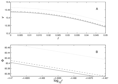
Figure 1: Behavior of $\Phi$ and $r$ along an outgoing ray (at fixed $u$) for various values of $N$. Upper panel (A): $v$ as a function of $r$. Lower panel (B): $\Phi$ as a function of $r$. In both panels dotted lines correspond to $N=10$, dashed lines to $N=20$, and solid lines to $N=40$, and the data are taken for $u=21.9$.

Figure 2 displays equi-spaced (in $u$) outgoing null rays (with constant values of $u$) in the $rv$-plane. The strong nonlinear dynamics is demonstrated by the rapid increase in the apparent horizon. All the rays which are not outside the event horizon and escape to infinity, either terminate at $r=0$ within a finite lapse of advanced time $v$ (type I), or approach a finite limiting value of $r$ as $v\to\infty$ of $r$ at large values of $v$ (type II).

The null portion of the singularity: Figure 3(A) shows the behavior of $r_{,v}$ along a type-II outgoing ray. At late times $r_{,v}\propto v^{-2}$. Figure 3(B) shows the behavior of $\Phi_{,v}$ along the same outgoing ray. At late times $\Phi_{,v}\propto v^{-1}$. This implies that along type-II rays $r$ indeed approaches a non-zero finite value as $v\to\infty$, but $\Phi$ diverges logarithmically in the same limit. This behavior is in sharp contrast with the behavior of $\Phi$ in the case of perturbations with compact support, where $\Phi$, too, approaches a non-zero finite value. We next check the detailed behavior of the fields along type-II rays. We find that type-II rays terminate (in the infinite future as $v\to\infty$) at a curvature singularity. This is demonstrated by Fig. 3(C), which shows the exponential increase in $R\equiv(R_{\alpha\beta}R^{\alpha\beta})^{1/2}$ along the same outgoing ray, $R_{\alpha\beta}$ being the Ricci tensor. (Notice that here $R$ is not the Ricci curvature scalar.) The finiteness of $r$ at the singular hypersurface suggests that the non-central portion of the singularity is deformationally weak.

Note that the late-time behavior of $r_{,v}$ and $\Phi_{,v}$, as is clear from Fig. 3, starts to dominate much earlier than in the case of perturbations of compact support. In particular, no quasi-normal modes (QNM) are visible. The reason for that is that the gradients of $\Phi$ decays here much slower than the tails in the case of perturbations of compact support. Specifically, $\Phi_{,v}$ decays here according to an inverse power-law with a smaller index than in the case of perturbations with compact support. (In the latter case the index is $4$ for spherical perturbations, whereas here we have an index of $1$.) Because the field is stronger, it starts dominating earlier, and overwhelms the rapidly-decaying oscillations of the QNM.

f2.eps

Figure 2: Outgoing null rays (with fixed values of $u$) in the $rv$-plane. The solid lines correspond to different fixed values of $u$, and the dotted line describes the apparent horizon, which approaches $u=21.07185$ at late values of advanced time $v$. The values of $u$ for which rays are shown (from right to left) are from $u=20.8$ to $22.7$ in equal increments of $\Delta u=0.1$.

f3.eps

Figure 3: Behavior of the fields and the curvature of spacetime along a type-II outgoing null ray. Upper panel (A): $r_{,v}$ as a function of $v$. Middle panel (B): $\Phi_{,v}$ as a function of $v$. Lower panel (C): $R$ as a function of $v$. The data are shown along $u=21.1$.

The spacelike portion of the singularity: Type-I rays terminate at a spacelike singularity. The spacelike singularity inside a spherical charged black hole which is perturbed by a scalar field was studied within a simplified homogeneous model in Ref. burko99 , where the pointwise behavior of the geometry and the field was found. It was also shown in burko99 that approaching the spacetime singularity, the fully nonlinear and inhomogeneous numerical solution (where the perturbation field had a compact support on the characteristic hypersurface) was in full agreement with the pointwise behavior. The study of the singularity in Ref. burko99 was local: no assumptions were made regarding the form of the perturbation field on the characteristic hypersurface. We thus expect that type-I rays terminate at a spacelike singularity whose pointwise behavior is well described by the singularity of Ref. burko99 . Assuming homogeneity, one finds approaching the spacelike singularity inside a spherical charged black hole with a scalar field, that

$$\Phi(r)=\sqrt{\beta+1}\ln r+O(r^{\beta})\,.$$ (8)

Here, $\beta>0$ is a constant (which numerically can be found to depend on $u$). Also, along an outgoing null ray one can show that, to the leading order in $v_{*}-v$,

$$r(u_{0},v)=[d^{2}/(\beta+1)]^{1/4}(v_{*}-v)^{1/2}\,,$$ (9)

where $d$ is a gauge-dependent quatity (which depends on the scaling of the temporal coordinate), and $v_{*}=v(r=0)$ along that null ray.

The agreement of our results with Eqs. (8) and (9) is already apparent from Fig. 1. Next, we check this agreement in greater detail. In Fig. 4(B) we show the behavior of the scalar field $\Phi$ as a function of $r(v)$ along a type-I outgoing null ray. This logarithmic behavior is consistent with Eq. (8). Along all type-I rays we find the same logarithmic divergence of $\Phi$, including along rays which initially are outside or inside the apparent horizon. (The only difference between different rays is that the slope of the graph, i.e., the value of the parameter $\beta$, changes from one ray to another.)

f4.eps

Figure 4: The scalar field $\Phi$ and the radial coordinate $r$ approaching the singularity along a type-I null ray. Upper panel (A): $v_{*}-v$ as a function of $r$. Lower panel (B): $\Phi$ as a function of $r$. The data are shown along the outgoing null ray at $u=21.9$.

Figure 4(A) displays $v_{*}-v$ as a function of $r$ along the same outgoing null ray. The asymptotic behavior approaching the singularity agrees very nicely with Eq. (9).

We conclude that the pointwise behavior at the singularity which we find in our simulations is well described by the singularity described in Ref. burko99 . Notice that this singularity is different from the Schwarzschild singularity: The former has $\beta>0$, and the latter has $\beta=-1$. This portion of the singularity then is scalar curvature, spacelike, and deformationally strong.

Conclusions: We studied the evolution of spacetime, and specifically the formation of curvature singularities, for a very simplied toy model of a spherical charged black hole, which is perturbed nonlinearly by a self-gravitating, spherical scalar field, which has non-compact support on the characteristic initial hypersurface. Although these perturbations are stronger than those which result from an initial profile with compact support (the gradient of the scalar field $\Phi$ decays at late times as $v^{-1}$ in our case, and as $v^{-4}$ in the case of perturbations with compact support) and consequently the evolution of spacetime and in particular of spacetime curvature is indeed dominated by the non-compact perturbations rather than by the perturbations due to the collapse, we find that a portion of the Cauchy horizon still survives as a non-central, null singularity, rather than being utterly destroyed and replaced by a central, spacelike singularity. The null generators of the Cauchy horizon contract with retarded time $u$, and eventually arrive at $r=0$, where the causal structure and the strength the singularity change: the central singularity is spacelike and deformationally strong. This situation and the global causal structure is therefore very similar to that of a black hole perturbed by a perturbation field with compact support, despite the different details of the dynamics.

The reason why the Cauchy horizon survived the introduction of non-compact perturbations as a null, non-central singularity is the following: We chose the characteristic field to be such, that although it is non-compact and does not belong to the same class of behavior on the event horizon at late advanced time as the tails, its gradient does. Specifically, along the event horizon $\Phi$ is logarithmic in advanced time. This certainly does not belong to the class of the tails, which decay as an inverse integral power of advanced time on the event horizon. However, $\phi_{,v}$ decays like $v^{-1}$ along the event horizon at late advanced time, such that it does belong to the same class as the gradients of the tails. (Note, that no tails would ever produce $n=1$, as $n$ is at least $3$ for all tails.) It is, in fact, $\phi_{,v}$ which is the important quantity, as curvature depends on the gradients of $\Phi$, rather than on $\Phi$ itself. This particular form of $\phi_{,v}$ implies that ${\cal R}$ can still be twice integrable approaching the Cauchy horizon.

We therefore conclude that by themselves, perturbations of non-compact support, even when they dominate the dynamics, are not sufficient to obliterate the null, non-central singularity at the Cauchy horizon. It remains an open question, however, whether other classes of non-compact perturbations behave similarly. The CBR perturbations, which are a generic source of perturbations for realistic black holes, are of particular interest. The energy influx of the CBR decays only on very long time scales due to the expansion of the universe (in a matter-dominated universe). (In a dark-energy dominated universe the influx of CBR energy decays faster.) It is interesting to investigate how the Cauchy horizon singularity is affected by such perturbation fields, and also to investigate which families of perturbing fields may destoy the null, non-central singularity.

I thank Karel Kuchař and Richard Price for discussions, and an anonymous referee for useful comments. This research was supported by the National Science Foundation through grant No. PHY-9734871.

References

- (1) For recent reviews see L. M. Burko and A. Ori, in Internal structure of black holes and spacetime singularities, edited by L. M. Burko and A. Ori (Institute of Physics, Bristol, 1997); P. R. Brady, Prog. Theor. Phys. Suppl. 136, 29 (1999).
- (2) E. Poisson and W. Israel, Phys. Rev. D 41, 1796 (1990).
- (3) A. Ori, Phys. Rev. Lett. 67, 789 (1991).
- (4) A. Ori, Phys. Rev. Lett. 68, 2117 (1992).
- (5) P. R. Brady and J. D. Smith, Phys. Rev. Lett. 75, 1256 (1995).
- (6) L. M. Burko, Phys. Rev. Lett. 79, 4958 (1997).
- (7) L. M. Burko and A. Ori, Phys. Rev. D 57, R7084 (1998).
- (8) L. M. Burko, Phys. Rev. D 60, 104033 (1999).
- (9) Notice that there is a misprint in Eq. (4) of L. M. Burko, Mod. Phys. Lett. A 14, 1015 (1999). The correct relation is given in Eq. (14) of Ref. burko99a .
- (10) R. H. Price, Phys. Rev. D 5, 2419 (1972).
- (11) C. J. S. Clarke and A. Królak, J. Geom. Phys. 2, 127 (1985).
- (12) L. M. Burko, Phys. Rev. D 55, 2105 (1997).
- (13) A. Ori, Phys. Rev. Lett. 83, 5423 (1999).
- (14) L. M. Burko and A. Ori, Phys. Rev. D 56, 7820 (1997).
- (15) L. M. Burko, Phys. Rev. D 59, 024011 (1999).