Black holes: A physical route to the Kerr metric

Abstract

As a consequence of Birkhoff’s theorem, the exterior gravitational field of a spherically symmetric star or black hole is always given by the Schwarzschild metric. In contrast, the exterior gravitational field of a rotating (axisymmetric) star differs, in general, from the Kerr metric, which describes a stationary, rotating black hole.

In this paper I discuss the possibility of a quasi–stationary transition from rotating equilibrium configurations of normal matter to rotating black holes.

1 Introduction: The Kerr black hole

The Kerr metric [1], in Boyer–Lindquist coordinates [2], is given by

$$ds^{2}=\Sigma\,(\frac{dr^{2}}{\Delta}+d\vartheta^{2})+W^{2}e^{-2\nu}(d\varphi-\omega\,dt)^{2}-e^{2\nu}dt^{2}$$ (1)

with

$$\Sigma=r^{2}+a^{2}\cos^{2}\vartheta,\quad\Delta=r^{2}-2Mr+a^{2},\quad W^{2}=\Delta\sin^{2}\vartheta,$$ (2)

$$e^{2\nu}=\frac{\Delta\Sigma}{(r^{2}+a^{2})^{2}-\Delta a^{2}\sin^{2}\vartheta}\quad\mbox{and}\quad\omega=\frac{2Mra}{\Delta\Sigma}\,e^{2\nu}.$$ (3)

It depends on two parameters, the total mass $M$ and the angular momentum $J=Ma$ (we assume $J\geq 0$ without loss of generality, and we use units where the velocity of light $c$ as well as Newton’s gravitational constant $G$ are equal to 1). The metric is stationary (independent of $t$) and axisymmetric (independent of $\varphi$). The horizon of the black hole is given by

$$r=r_{+}\equiv M+\sqrt{M^{2}-a^{2}},$$ (4)

the larger root of the quadratic equation $\Delta=0$. Note that the Kerr metric describes a black hole only if

$$a\leq M\quad(J\leq M^{2})$$ (5)

is satisfied. The boundary of the ‘ergosphere’ is characterized by

$$r=r_{0}(\vartheta)\equiv M+\sqrt{M^{2}-a^{2}\cos^{2}\vartheta}.$$ (6)

Within the ergosphere ($r_{+}<r<r_{0}$) any observer must rotate in the same direction as the black hole ($d\varphi/dt>0$).

It is interesting to discuss circular orbits of test particles in the ‘equatorial plane’ $\vartheta=\pi/2$. Their angular velocity is given by

$$\Omega=\pm\frac{\sqrt{M}}{r^{3/2}\pm a\sqrt{M}}\quad,$$ (7)

where the upper sign characterizes direct orbits (corotating with the black hole) and the lower sign holds for retrograde (counterrotating) orbits. The circular orbits exist only for $r>r_{\rm ph}$, with the ‘photon orbit’

$$r_{\rm ph}=2M\left\{1+\cos\left[\frac{2}{3}\arccos\left(\mp\frac{a}{M}\right)\right]\right\}.$$ (8)

The orbits are bound for $r>r_{\rm mb}$, with the ‘marginally bound orbit’

$$r_{\rm mb}=2M\mp a+2M^{1/2}(M\mp a)^{1/2}.$$ (9)

(A particle in an unbound orbit will, under the influence of an infinitesimal outward perturbation, escape to infinity.) The orbits are stable for $r>r_{\rm ms}$, with the ‘marginally stable orbit’

$$r_{\rm ms}=M\left\{3+Z_{2}\mp\left[(3-Z_{1})(3+Z_{1}+2Z_{2})\right]^{1/2}\right\}$$ (10)

$$\mbox{where}\quad Z_{1}=1+\left(1-\frac{a^{2}}{M^{2}}\right)^{1/3}\left[\left(1+\frac{a}{M}\right)^{1/3}+\left(1-\frac{a}{M}\right)^{1/3}\right]$$ (11)

$$\mbox{and}\quad Z_{2}=\left(3\frac{a^{2}}{M^{2}}+Z_{1}^{2}\right)^{1/2}.$$ (12)

These results on circular orbits of test particles were derived by Bardeen et al. [3], see also [4].

2 Limiting cases

The two limiting cases of the Kerr black hole are $a=0$ ($J=0$), the nonrotating (Schwarzschild) black hole, and $a=M$ ($J=M^{2}$), the maximally rotating (extreme Kerr) black hole. For $a=0$ the horizon is given by $r_{+}=2M$ (‘Schwarzschild radius’) and no ergosphere exists. For $a=M$ one has $r_{+}=M$ and the ergosphere extends up to $r_{0}(\pi/2)=2M$ in the equatorial plane. The values of the characteristic radii $r_{\rm ph}$, $r_{\rm mb}$ and $r_{\rm ms}$ discussed above are given in Table 1.

Table 1: Photon orbit, marginally bound orbit and marginally stable orbit for the Schwarzschild black hole and for the extreme Kerr black hole. In the latter case one has to distinguish between direct and retrograde orbits.

	$r_{\rm ph}$	$r_{\rm mb}$	$r_{\rm ms}$
$a=0$	3M	4M	6M
$a=M$ (direct)	M	M	M
$a=M$ (retrograde)	4M	$(3+2\sqrt{2})$M	9M

In the extreme case $r_{\rm ph}^{(d)}$, $r_{\rm mb}^{(d)}$ and $r_{\rm ms}^{(d)}$ [the $(d)$ indicates direct orbits] all coincide with $r_{+}=M$. However, defining proper radial distances according to

$$\delta(r_{1},r_{2})=\int\limits_{r_{1}}^{r_{2}}\sqrt{g_{rr}}\,dr,\quad g_{rr}=\frac{\Sigma}{\Delta}\quad,$$ (13)

one finds [3]

$$\lim_{a\to M}\delta(r_{+},r_{\rm ph}^{(d)})=\frac{M}{2}\ln 3,\quad\lim_{a\to M}\delta(r_{+},r_{\rm mb}^{(d)})=M\ln(1+\sqrt{2})$$ (14)

$$\mbox{and}\quad\lim_{a\to M}\delta(r_{+},r_{\rm ms}^{(d)})=\infty.$$ (15)

Moreover, because of the double zero of $\Delta$ at $r=M$ for the extreme Kerr metric, one obtains

$$\delta(M,r)=\infty\quad\mbox{for any}\quad r>M.$$ (16)

This means, the horizon (as well as $r_{\rm ph}^{(d)}$, $r_{\rm mb}^{(d)}$ and $r_{\rm ms}^{(d)}$ !) has an infinite proper radial distance from any point in the ‘exterior’ region $r>M$. On the other hand, the proper time of an infalling particle starting at some $r>M$ needed to reach the horizon remains finite.

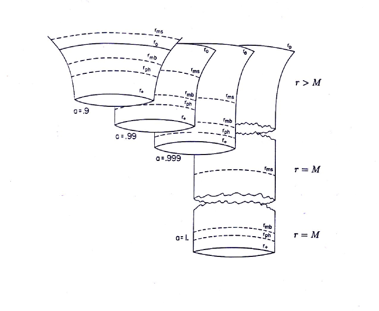
Figure 1: Embedding diagrams of the $r\geq r_{+}$ part of the ‘plane’ $\vartheta=\pi/2$, $t={\rm constant}$ of the Kerr metric approaching the limit $a=M$ (from Bardeen et al. [3]; $a$ is given in units of $M$). The positions of the direct orbits $r_{\rm ph}$, $r_{\rm mb}$, $r_{\rm ms}$ and of the boundary $r_{0}$ of the ergosphere are shown.

The geometrical situation can nicely be illustrated by embedding the $r\geq r_{+}$ part of the ‘plane’ $\vartheta=\pi/2$, $t={\rm constant}$ into three–dimensional Euclidean space [3], see Fig. 1. In the limit $a=M$ an infinitely long ‘throat’ characterized by $r=M$ (circumference: $4\pi M$) appears. The horizon is situated at the bottom and the direct orbits corresponding to $r_{\rm ph}^{(d)}$, $r_{\rm mb}^{(d)}$ and $r_{\rm ms}^{(d)}$ are located at different places along the throat. However, the proper time of an infalling particle needed for passing through this throat, is zero. Bardeen and Horowitz [5] have studied the ‘throat geometry’ ($r=M$) by means of the coordinate transformation

$$\tilde{r}=\frac{r-M}{\lambda},\quad\tilde{\vartheta}=\vartheta,\quad\tilde{\varphi}=\varphi-\Omega_{\rm H}t,\quad\tilde{t}=\lambda t$$ (17)

in the limit $\lambda\to 0$. Note that

$$\omega(r_{+},\vartheta)=\Omega_{\rm H}={\rm constant}$$ (18)

defines the ‘angular velocity of the horizon’. For the extreme Kerr black hole it is given by

$$\Omega_{\rm H}=\frac{1}{2M}.$$ (19)

One obtains

$$ds^{2}=M^{2}(1+\cos^{2}\tilde{\vartheta})\left(\frac{d\tilde{r}^{2}}{\tilde{r}^{2}}+d\tilde{\vartheta}^{2}-\frac{\tilde{r}^{2}d\tilde{t}^{2}}{4M^{4}}\right)+\frac{4M^{2}\sin^{2}\tilde{\vartheta}}{1+\cos^{2}\tilde{\vartheta}}\left(d\tilde{\varphi}+\frac{\tilde{r}d\tilde{t}}{2M^{2}}\right)^{2}.$$ (20)

This represents a completely nonsingular vacuum solution of Einstein’s equations which is geodesically complete but no longer asymptotically flat [5]. The area of all surfaces $\tilde{r}={\rm constant}$, $\tilde{t}={\rm constant}$ is $8\pi M^{2}$ and equal to the area of the horizon of the extreme Kerr black hole. In addition to $\partial/\partial\tilde{t}$ and $\partial/\partial\tilde{\varphi}$ the metric (20) has two more Killing fields [8, 5]:

$$\left(\frac{\tilde{t}^{2}}{2}+\frac{1}{8\tilde{r}^{2}\Omega_{\rm H}^{4}}\right)\frac{\partial}{\partial\tilde{t}}-\tilde{r}\tilde{t}\frac{\partial}{\partial\tilde{r}}-\frac{1}{2\tilde{r}\Omega_{\rm H}^{2}}\frac{\partial}{\partial\tilde{\varphi}},\quad\tilde{t}\frac{\partial}{\partial\tilde{t}}-\tilde{r}\frac{\partial}{\partial\tilde{r}}.$$ (21)

3 Idealized routes to black holes

A famous idealized route to the Schwarzschild black hole is the spherically symmetric dust collapse (‘Oppenheimer–Snyder collapse’) [9, 10]. Bardeen and Wagoner [11] have shown approximately that a uniformly rotating disk of dust allows a quasi–stationary transition (parametric collapse) towards the extreme Kerr black hole. This has been confirmed by the exact solution to the disk problem [12, 13], see also [6]. Here the main results will be reviewed.

The line element for any stationary, axisymmetric, purely rotating perfect–fluid configuration may be written in Lewis–Papapetrou coordinates as

$$ds^{2}=e^{2\alpha}(d\varrho^{2}+d\zeta^{2})+W^{2}e^{-2\nu}(d\varphi-\omega\,dt)^{2}-e^{2\nu}dt^{2}.$$ (22)

The four functions $\alpha$, $W$, $\nu$ and $\omega$ depend on $\varrho$ and $\zeta$ only. Along the symmetry axis, $\varrho=0$, the condition of elementary flatness requires

$$\lim\limits_{\varrho\to 0}\frac{W}{\varrho}e^{-(\alpha+\nu)}=1$$ (23)

and at infinity ($\varrho^{2}+\zeta^{2}\to\infty$) the asymptotic line element has to take the Minkowski form in cylindrical coordinates,

$$ds^{2}=d\varrho^{2}+d\zeta^{2}+\varrho^{2}d\varphi^{2}-dt^{2},$$ (24)

$$\mbox{i.e.,}\quad\alpha\to 0,\quad W\to\varrho,\quad\nu\to 0,\quad\omega\to 0.$$ (25)

An equivalent form of (22) is

$$ds^{2}=e^{-2U}\left[e^{2k}(d\varrho^{2}+d\zeta^{2})+W^{2}d\varphi^{2}\right]-e^{2U}(dt+A\,d\varphi)^{2}$$ (26)

$$\mbox{with}\quad\alpha=k-U,\quad W^{-1}e^{2\nu}\pm\omega=\left(W\,e^{-2U}\mp A\right)^{-1}.$$ (27)

For the disk of dust one obtains

$$W\equiv\varrho$$ (28)

and the whole problem can be formulated as a boundary value problem [12] of the Ernst equation

$$(\Re f)(f,_{\rho\rho}+f,_{\zeta\zeta}+\rho^{-1}f,_{\rho})=f,_{\rho}^{2}+f,_{\zeta}^{2}.$$ (29)

The metric can easily be obtained from the complex Ernst potential

$$f=e^{2U}+ib$$ (30)

whose real part is equal to $e^{2U}$. The functions $A$ and $k$ can be calculated by integration:

$$A(\varrho,\zeta)=\int\limits_{0}^{\rho}\tilde{\rho}e^{-4U}b,_{\zeta}d\tilde{\rho},\quad k(\varrho,\zeta)=\int\limits_{0}^{\rho}\tilde{\rho}\left[U,_{\tilde{\rho}}^{2}-U,_{\zeta}^{2}+\frac{e^{-4U}}{4}(b,_{\tilde{\rho}}^{2}-b,_{\zeta}^{2})\right]d\tilde{\rho}.$$ (31)

[In the integrands, one has $U=U(\tilde{\rho},\zeta)$ and $b=b(\tilde{\rho},\zeta)$.] Like the Kerr metric, the solution for a uniformly rotating disk of dust depends on two parameters, the total mass $M$ and the angular momentum $J$. In contrast to (5) the relation

$$J\geq M^{2}$$ (32)

holds for the disk of dust. Instead of $M$ and $J$ other parameter pairs can be used. In the following, the solution is represented in terms of the two parameters $\varrho_{0}$ (coordinate radius of the disk) and $\mu$, where $\mu$ is related to $\Omega$ (angular velocity of the disk) by

$$\mu=2\Omega^{2}\varrho_{0}^{2}e^{-2V_{0}};\quad V_{0}\equiv U(\varrho=0,\zeta=0).$$ (33)

The Ernst potential is given by hyperelliptic integrals [13]:

$$f=\exp\left\{\int\limits_{K_{1}}^{K_{a}}\frac{K^{2}dK}{Z}+\int\limits_{K_{2}}^{K_{b}}\frac{K^{2}dK}{Z}-v_{2}\right\},$$ (34)

with

$$Z=\sqrt{(K+iz)(K-i\bar{z})(K^{2}-K_{1}^{2})(K^{2}-K_{2}^{2})},\quad z=\varrho+i\zeta,$$ (35)

$$K_{1}=-\bar{K}_{2}=\rho_{0}\sqrt{\frac{i-\mu}{\mu}}\quad(\Re K_{1}<0,\,\,\mbox{a bar denotes complex conjugation}).$$ (36)

The upper integration limits $K_{a}$ and $K_{b}$ in (34) have to be calculated from

$$\int\limits_{K_{1}}^{K_{a}}\frac{dK}{Z}+\int\limits_{K_{2}}^{K_{b}}\frac{dK}{Z}=v_{0},\quad\int\limits_{K_{1}}^{K_{a}}\frac{KdK}{Z}+\int\limits_{K_{2}}^{K_{b}}\frac{KdK}{Z}=v_{1},$$ (37)

where the functions $v_{0}$, $v_{1}$ and $v_{2}$ in (37) and (34) are given by

$$v_{0}=\int\limits_{-i\rho_{0}}^{+i\rho_{0}}\frac{H}{Z_{1}}dK,\quad v_{1}=\int\limits_{-i\rho_{0}}^{+i\rho_{0}}\frac{H}{Z_{1}}KdK,\quad v_{2}=\int\limits_{-i\rho_{0}}^{+i\rho_{0}}\frac{H}{Z_{1}}K^{2}dK,$$ (38)

$$H=\frac{\mu\ln\left[\sqrt{1+\mu^{2}(1+K^{2}/\rho_{0}^{2})^{2}}+\mu(1+K^{2}/\rho_{0}^{2})\right]}{\pi i\rho_{0}^{2}\sqrt{1+\mu^{2}(1+K^{2}/\rho_{0}^{2})^{2}}}\qquad(\Re H=0),$$ (39)

$$Z_{1}=\sqrt{(K+iz)(K-i\bar{z})}\qquad(\Re Z_{1}<0\,\,\mbox{for $\rho$, $\zeta$ outside the disk}).$$ (40)

In (38) one has to integrate along the imaginary axis. The integrations from $K_{1}$ to $K_{a}$ and from $K_{2}$ to $K_{b}$ in (34) and (37) have to be performed along the same paths in the two–sheeted Riemann surface associated with $Z(K)$. The problem of finding $K_{a}$ and $K_{b}$ from (37) is a special case of Jacobi’s inversion problem. It generalizes the definition of elliptic functions and can be solved in terms of hyperelliptic theta functions ([14, 15], see also [16, 17, 18]). Using a formula for Abelian integrals of the third kind derived by Riemann (see [16]) it is also possible to express the Ernst potential $f$ directly in terms of theta functions [19]. On the symmetry axis ($\rho=0$) and in the plane of the disk ($\zeta=0$) all integrals in (34) and (37) reduce to elliptic ones [20].

The solution has a positive surface mass–density [20] and it is regular everywhere outside the disk – provided

$$0<\mu<\mu_{0}=4.62966184\dots$$ (41)

(for $\mu>\mu_{0}$ one or more singular rings appear in the plane $\zeta=0$, outside the disk). The parameter $V_{0}$ [see (33)] depends on $\mu$ alone [20]:

$$V_{0}=-\frac{1}{2}\sinh^{-1}\left\{\mu+\frac{1+\mu^{2}}{\wp[I(\mu);\frac{4}{3}\mu^{2}-4,\frac{8}{3}\mu(1+\mu^{2}/9)]-\frac{2}{3}\mu}\right\},$$ (42)

$$I(\mu)=\frac{1}{\pi}\int\limits_{0}^{\mu}\frac{\ln(x+\sqrt{1+x^{2}})dx}{\sqrt{(1+x^{2})(\mu-x)}}$$ (43)

with the Weierstrass function $\wp$ defined by

$$\int\limits_{\wp(x;g_{2},g_{3})}^{\infty}\frac{dt}{\sqrt{4t^{3}-g_{2}t-g_{3}}}=x.$$ (44)

The range $0<\mu<\mu_{0}$ corresponds to $0>V_{0}>-\infty$. [$\mu_{0}$ is the first zero of the denominator in (42).] From (33) and (42) one obtains the relation $\Omega(\mu,\rho_{0})$.

Figure 2: Formation of the ergosphere (from [22]). It appears for $\mu>\mu_{\rm e}=1.68849\dots$ and has a toroidal shape. The horizontal line represents the disk. For $\mu\to\mu_{0}$ the ergosphere is that of the extreme Kerr black hole.

Whereas $\mu\ll 1$ characterizes the Newtonian limit (the ‘Maclaurin disk’), $\mu\to\mu_{0}$ leads to the announced black hole limit:

For $\mu\to\mu_{0}$ one obtains

$$\frac{M^{2}}{J}\to 1,\quad 2\Omega M\to 1,\quad\Omega\varrho_{0}\to 0,\quad\mbox{which means, for finite $M$,}$$ (45)

$$\varrho_{0}\to 0.$$ (46)

For the further discussion, we introduce spherical–like coordinates $R$, $\vartheta$:

$$\varrho=R\,\sin\vartheta,\quad\zeta=R\,\cos\vartheta.$$ (47)

The disk ($\zeta=0$, $\varrho\leq\varrho_{0}$) shrinks to the origin $R=0$ of the coordinate system. For $R\neq 0$, the disk metric becomes exactly the $r>M$ part of the extreme Kerr metric given by (1) with $a=M$ ($\Omega_{\rm H}=\Omega=1/2M$) and

$$r=R+M.$$ (48)

This can be shown as follows [6, 21]:

Let us first rewrite (34) and (37) in the equivalent form

$$f=\exp\left\{\,\int\limits_{K_{b}}^{K_{a}}\frac{K^{2}dK}{Z}-\tilde{v}_{2}\right\},\quad\int\limits_{K_{b}}^{K_{a}}\frac{dK}{Z}=\tilde{v}_{0},\quad\int\limits_{K_{b}}^{K_{a}}\frac{KdK}{Z}=\tilde{v}_{1},$$ (49)

with

$$\tilde{v}_{n}=v_{n}-\int\limits_{K_{1}}^{K_{2}}\frac{K^{n}dK}{Z}\quad(n=0,1,2).$$ (50)

($K_{b}$ is now on the other sheet of the Riemann surface.) In the limit $\mu\to\mu_{0}$ one obtains for $R>0$, using (33) and (42),

$$\tilde{v}_{0}=\frac{2\Omega}{R}-\frac{\pi i\cos\vartheta}{2R^{2}},\quad\tilde{v}_{1}=-\frac{\pi i}{2R},\quad\tilde{v}_{2}=0$$ (51)

(modulo periods). In the above integrals from $K_{b}$ to $K_{a}$, $Z$ can be replaced by $Z=K^{2}\sqrt{(K+iz)(K-i\bar{z})}$ since $K_{1}$ and $K_{2}$ both tend to zero [cf. (36)]. Hence, all integrals become elementary and the unique result is

$$f=\frac{2\Omega R-1-i\cos\vartheta}{2\Omega R+1-i\cos\vartheta}\qquad(R>0),$$ (52)

which is the Ernst potential of the extreme Kerr solution. Note that $R=0$ ($r=M$) characterizes the horizon (and the throat) of the extreme Kerr black hole.

In Fig. 2 the formation of the ergosphere is shown [22]. In the limit $\mu\to\mu_{0}$ the ergosphere of the extreme Kerr black hole appears. Indeed, from (6), (47) and (48) one finds the following equation for the boundary of the extreme Kerr ergosphere in the (Weyl) coordinates $\varrho$, $\zeta$ (note that $2M=1/\Omega$):

$$\left(\frac{\varrho_{\rm e}}{2M}-\frac{1}{4}\right)^{2}+\left(\frac{\zeta_{\rm e}}{2M}\right)^{2}=\frac{1}{16}.$$ (53)

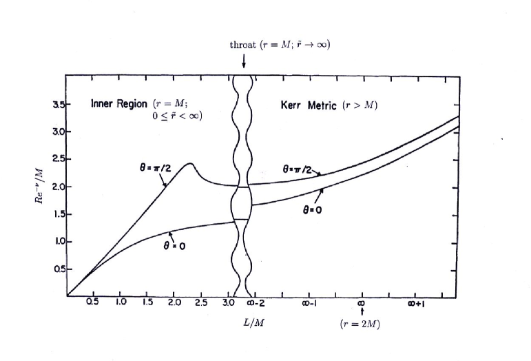
Figure 3: The $\mu\to\mu_{0}$ disk metric (from Bardeen and Wagoner [11], slightly modified). The ordinate shows the values of the function $R\,e^{-\nu}/M$ for $\vartheta=0$ (axis of symmetry) and for $\vartheta=\pi/2$ (equatorial plane). The abscissa shows $L/M$ where $L$ is the proper radial distance from the center of the disk. All points in the ‘exterior’ ($r>M$) region have an infinite proper distance to the ‘inner’ ($r=M$) region which contains the disk and its surroundings. The point ‘$L/M=\infty$’ corresponds to the coordinate value $r=2M$, ‘$L/M=\infty+x$’ means $\delta(2M,r)=xM$, cf. Eq. (13).

A completely different limit of the space–time, for $\mu\to\mu_{0}$, is obtained for finite values of $R/\rho_{0}$ (corresponding to the previously excluded $R=0$). Therefore, we consider a coordinate transformation [11]

$$\tilde{r}=e^{-V_{0}}R,\quad\tilde{\vartheta}=\vartheta,\quad\tilde{\varphi}=\varphi-\Omega t,\quad\tilde{t}=e^{V_{0}}t.$$ (54)

(Note that finite $R/\rho_{0}$ correspond to finite $\tilde{r}$ in the limit.) For $\mu<\mu_{0}$, this is nothing but the transformation to the corotating system combined with a rescaling of $R$ and $t$. The transformed Ernst potential $\tilde{f}$ is related to the Ernst potential $f^{\prime}$ in the corotating system ($R^{\prime}=R$, $\vartheta^{\prime}=\vartheta$, $\varphi^{\prime}=\varphi-\Omega t$, $t^{\prime}=t$) according to $\tilde{f}=f^{\prime}\exp(-2V_{0})$, i.e.,

$$\frac{\tilde{f}}{\tilde{r}^{2}}=\frac{f^{\prime}}{R^{2}}\quad\mbox{for}\quad\mu<\mu_{0}.$$ (55)

However, for $\mu\to\mu_{0}$, the solutions $f^{\prime}$ (finite $R>0$) and $\tilde{f}$ (finite $\tilde{r}$) separate from each other. (A similar phenomenon has been observed by Breitenlohner et al. for some limiting solutions of the static, spherically symmetric Einstein–Yang–Mills–Higgs equations [23].) For finite $R>0$, the extreme Kerr solution arises, while finite $\tilde{r}$ lead to a solution which still describes a disk, with finite coordinate radius

$$\tilde{\varrho}_{0}=\lim\limits_{\mu\to\mu_{0}}(e^{-V_{0}}\varrho_{0})=\sqrt{2\mu_{0}}\,M.$$ (56)

Note that the proper radius of the disk remains finite in the limit $\mu\to\mu_{0}$ as well. Its circumference is $4\pi M\sqrt{\mu_{0}/2-1}$ which is larger than the circumference $4\pi M$ of the extreme Kerr throat. The metric corresponding to $\tilde{f}$ (which can be expressed in terms of theta functions) is regular everywhere outside the disk, but it is not asymptotically flat. The space–time structure of both solutions ($f^{\prime}$ and $\tilde{f}$) coincides at $R\to 0$ (the throat) and $\tilde{r}\to\infty$ (spatial infinity). The relation (55) survives in the form

$$\lim\limits_{\tilde{r}\to\infty}\,\frac{\tilde{f}}{\tilde{r}^{2}}=\lim\limits_{R\to 0}\,\frac{f^{\prime}}{R^{2}}\quad\mbox{as}\quad\mu\to\mu_{0}.$$ (57)

[The limits have to be taken consistently with (54).] The Ernst potential $f^{\prime}$ of the extreme Kerr solution in the corotating system reads

$$f^{\prime}=-\Omega^{2}R^{2}\left[\frac{2(1+i\cos\vartheta)^{2}}{2\Omega R+1-i\cos\vartheta}+\sin^{2}\vartheta\right].$$ (58)

Accordingly, for $\mu=\mu_{0}$ and $\tilde{r}\to\infty$,

$$\tilde{f}\to\tilde{f}_{\rm as}=-\Omega^{2}\tilde{r}^{2}\left[\frac{2(1+i\cos\tilde{\vartheta})^{2}}{1-i\cos\tilde{\vartheta}}+\sin^{2}\tilde{\vartheta}\right].$$ (59)

Note that $\tilde{f}_{\rm as}$ belongs to the family of solutions to the Ernst equation of the type $f=R^{k}Y_{k}(\cos\vartheta)$ presented by Ernst [7]. The corresponding asymptotic line element is given by the extreme Kerr throat geometry (20). These exact results [6] confirm the picture of the extreme relativistic limit of the rotating disk developed by Bardeen and Wagoner [11]. Fig. 3 (taken from [11]) combines the two limits of the disk space–time for $\mu\to\mu_{0}$. The abscissa characterizes the proper radial distance $L$ from the center of the disk:

$$L=\int\limits_{0}^{\tilde{r}}\sqrt{g_{\tilde{r}\tilde{r}}}\,d\tilde{r}=\int\limits_{0}^{R}\sqrt{g_{RR}}\,dR.$$ (60)

The two ‘worlds’ are separated by the ‘throat region’ which plays the role of infinity for the ‘inner region’. From the point of view of the ‘exterior region’ (the $r>M$ part of the extreme Kerr metric) it is the extreme Kerr throat as discussed in Section 2. Note that the plotted quantity $R\,e^{-\nu}/M$, for $\vartheta=\pi/2$, is equal to $\sqrt{g_{\varphi\varphi}}/M$, which is just the circumferential radius of a circle in the equatorial plane (concentrical to the disk) divided by $M$. The value of 2 in the throat region corresponds to the throat’s circumference $4\pi M$.

Figure 4: Parametric collapse of the rigidly rotating disk of dust (from [12]). The diagram shows the relation between $2\Omega M$ and $M^{2}/J$ for the disk of dust and for the Kerr black hole [$\Omega=\Omega_{\rm H}$, cf. Eq. (18)]. The dashed line corresponds to the Newtonian disk solution (the Maclaurin disk) where $2\Omega M=(9\pi^{2}/125)(M^{2}/J)^{3}$.

The quasi–stationary transition from the disk to the Kerr black hole is illustrated in Fig. 4 where $2\Omega M$ is shown in dependence on the parameter $M^{2}/J$ [12]. The limit $M^{2}/J\to 1$ (from the left) corresponds to the limit $\mu\to\mu_{0}$ discussed above. The ‘exterior’ metric becomes the $r>r_{+}$ part of the extreme Kerr metric. For $M^{2}/J>1$ no disk solution exists and a genuine Kerr black hole forms. This transition (parametric collapse) from the disk to the Kerr black hole is continuous in the ‘exterior region’. In particular, all multipole moments behave continuously, see [24].

4 From stars to black holes

The exterior metric of a spherically symmetric star, even in the case of (dynamic) collapse, is always the Schwarzschild metric. This is a consequence of Birkhoff’s theorem [25]. Therefore, the spherically symmetric collapse of a sufficiently massive, non–rotating star at the end of its life leads quite naturally to a Schwarzschild black hole, as in the idealized Oppenheimer–Snyder case. On the other hand, a continuous quasi–static transition from stars to black holes is not possible. The surface of a star cannot be identical with the horizon of a black hole since the horizon is a null–hypersurface. Under the quite reasonable assumption that the mass–energy density does not increase outwards in the star, one can show that the radius $r_{*}$ of a spherically symmetric, static star (in Schwarzschild coordinates) always satisfies

$$r_{*}>\frac{9}{8}\,r_{+},$$ (61)

where $r_{+}=2M$ is the corresponding Schwarzschild radius (see [26], for example). Thus, at most the $r>(9/8)r_{+}$ part of the Schwarzschild vacuum metric is relevant outside static stars and the black hole state can only be reached dynamically.

For rotating stars, the situation is different in both previously mentioned respects. Firstly, the exterior metric is not the Kerr metric in general. (There is no analogue to Birkhoff’s theorem.) It is general belief, based on Penrose’s cosmic censureship conjecture combined with the black hole uniqueness theorems, cf. [27], that the (dynamic) collapse of a rotating star leads asymptotically ($t\to\infty$) to the Kerr black hole, i.e., to the Kerr metric outside the horizon. This has not yet been proved, however. But secondly, a continuous quasi–stationary route from rotating stars to rotating black holes via the extreme Kerr metric seems possible — as in the idealized (and certainly unstable) case of the rigidly rotating disk of dust. The problem of the impossible identity of the star’s surface with the horizon would be circumvented by the ‘throat region’, and the whole $r>r_{+}$ part of the extreme Kerr metric could be relevant in the ‘exterior region’, as discussed above. Results on differentially rotating disks of dust [28, 29] give some evidence that the extreme Kerr limit is a generic possibility. General relativistic, rotating stellar models can only be treated by numerical methods so far. However, the recently achieved progress in accuracy by many orders of magnitude [30] justifies the hope of finding a more realistic, quasi–stationary route to the Kerr metric.

I would like to thank M. Ansorg, A. Kleinwächter, G. Neugebauer and D. Petroff for many valuable discussions.

References

[1] R.P. Kerr, Phys. Rev. Lett. 11 (1963) 237
[2] R.H. Boyer and R.W. Lindquist, J. Math. Phys. 8 (1967) 265
[3] J.M. Bardeen, W.H. Press, and S.A. Teukolsky, Astrophys. J.
178 (1972) 347
[4] S.L. Shapiro and S.A. Teukolsky, Black Holes, White Dwarfs,
and Neutron Stars. The Physics of Compact Objects, John Wiley & Sons,
New York 1983
[5] J. Bardeen and G.T. Horowitz, Phys. Rev. D 60 (1999) 104030
[6] R. Meinel, in Recent Developments in Gravitation and
Mathematical Physics edited by A. García, C. Lämmerzahl, A. Macías,
T. Matos,
and D. Nuñez, Science Network Publishing, Konstanz 1998 (gr-qc/9703077)
[7] F.J. Ernst, J. Math. Phys. 18 (1977) 233
[8] T. Wolf, Computer Phys. Commun. 115 (1998) 316
[9] R.C. Tolman, Proc. Nat. Acad. Sci. U.S. 20 (1934) 169
[10] J.R. Oppenheimer and H. Snyder, Phys. Rev. 56 (1939) 455
[11] J.M. Bardeen and R.V. Wagoner, Astrophys. J. 167 (1971) 359
[12] G. Neugebauer and R. Meinel, Astrophys. J. 414 (1993) L97
[13] G. Neugebauer and R. Meinel, Phys. Rev. Lett. 75 (1995) 3046
[14] A. Göpel, Crelle’s J. für Math. 35 (1847) 277
[15] G. Rosenhain, Crelle’s J. für Math. 40 (1850) 319
[16] H. Stahl, Theorie der Abel’schen Funktionen, Teubner,
Leipzig 1896
[17] A. Krazer, Lehrbuch der Thetafunktionen, Teubner, Leipzig
1903
[18] E.D. Belokolos, A.I. Bobenko, V.Z. Enol’skii, A.R. Its and
V.B. Matveev, Algebro-Geometric Approach to Nonlinear Integrable
Equations, Springer, Berlin 1994
[19] G. Neugebauer, A. Kleinwächter and R. Meinel, Helv. Phys. Acta
69 (1996) 472
[20] G. Neugebauer and R. Meinel, Phys. Rev. Lett. 73 (1994) 2166
[21] R. Meinel, Ann. Phys. (Leipzig) 9 (2000) 335
[22] R. Meinel and A. Kleinwächter, Einstein Studies (Birkhäuser)
6 (1995) 339
[23] P. Breitenlohner, P. Forgács and D. Maison,
Nucl. Phys. B 442 (1995) 126
[24] A. Kleinwächter, R. Meinel and G. Neugebauer, Phys. Lett. A
200 (1995) 82
[25] G.D. Birkhoff, Relativity and Modern Physics,
Harvard University Press, Cambridge (USA) 1923
[26] S. Weinberg, Gravitation and Cosmology, Wiley, New York
1972
[27] S.W. Hawking and G.F.R. Ellis, The Large Scale Structure
of Space–Time, Cambridge University Press, Cambridge (UK) 1973
[28] M. Ansorg and R. Meinel, Gen. Rel. Grav. 32 (2000) 1365
[29] M. Ansorg, Gen. Rel. Grav. 33 (2001) 309
[30] M. Ansorg, A. Kleinwächter and R. Meinel, Astron. Astrophys.
381 (2002) L49