The 550 AU Mission: A Critical Discussion

Abstract

We have studied the science rationale, goals and requirements for a mission aimed at using the gravitational lensing from the Sun as a way of achieving high angular resolution and high signal amplification. We find that such a mission concept is plagued by several practical problems. Most severe are the effects due to the plasma in the solar atmosphere which cause refraction and scattering of the propagating rays. These effects limit the frequencies that can be observed to those above $\sim$100-200 GHz and moves the optical point outwards beyond the vacuum value of $\geq$ 550 AU. Density fluctuations in the inner solar atmosphere will further cause random pathlength differences for different rays. The corrections for the radiation from the Sun itself will also be a major challenge at any wavelength used. Given reasonable constraints on the spacecraft (particularly in terms of size and propulsion) source selection as well as severe navigational constraints further add to the difficulties for a potential mission.

1 Background

General relativity (GR) predicts that light will be deflected by any massive object; an effect first experimentally confirmed by Eddington (1919). As a consequence, a far away object will act as a lens because the deflected rays from the two sides of the lensing mass converge. This is a well known effect and has been observed over cosmological distances (Blandford and Narayan, 1992) where relatively nearby galaxies, or even clusters of galaxies, act as gravitational lenses for background galaxies, and in our Galaxy where micro-lensing of stars in the Galactic bulge or in the Magellanic clouds are caused by intervening (sub-)stellar bodies (Paczynski, 1996). Even though these studies can yield a wide variety of important information in many branches of astronomy, we are left at the mercy of Nature in the selection of sources. This drawback could in principle be overcome if we could move a spacecraft to the location of the focus of a gravitational lens due to some nearby object. As can be seen from below, of the solar system bodies, only the Sun is massive enough that the focus of its gravitational deflection is within range of a realistic mission. The gravitational lens effect of a spherical star for astronomical observations of distant objects has been studied by a number of authors (Refsdal, 1965; Bliokh and Minakov, 1975; Herlt and Stephani, 1976). The specific use of the Sun for that purpose was first proposed in 1979 by von Eshleman, whose original ‘study’ was aimed at interstellar communication with a single pre-determined pointing at long wavelengths. Subsequent discussions include those of Kraus (1986) and Heidmann and Maccone (1994). The main attraction of this technique is the high amplifications (gain, in astronomy nomenclature) which can be achieved (see Kraus (1986)). However, in these studies, several effects of importance to a possible implementation of such observations were neglected, mainly those due to the solar plasma and the brightness of the Sun. Herein, we give a brief review of the subject and present a preliminary investigation of some of the previously ignored effects. We also discuss possible observing strategies and source selection.

As with any space mission aimed at reaching distances outside of the solar system there are a large number of in situ measurements which can be performed during cruise. Given a suitable suite of instruments, studies of the heliosphere and its termination as well as the local interstellar medium can be performed. We briefly summarize some of the possible areas of cruise science addressed in the literature. Further possible secondary science objectives, such as VLBI and parallax measurements, will not be addressed.

The paper organized as follows: In Section 2 we discuss the basic parameters of the solar gravitational lens: the optical distance, the amplification and the gain. We also address the issue of solar plasma contribution to the total effect. In Section 3 we discuss the observational considerations for a concept of solar gravitational telescope. We present the ”pros” and ”cons” for a possible mission designed to utilize the solar gravitational lens for any scientific application. In Section 4 we present possible scientific program for the mission during its cruise phase. We conclude with Section 5, where we present our conclusions and recommendations related to the possibility of utilizing the solar gravitational lens in the future.

2 The Sun as a gravitational lens

2.1 GR lensing by a massive object in vacuum

It is well-known that light rays passing by a gravitating body are deflected by the body’s gravitational field (see (Paczynski, 1996) and references therein). The largest contribution to the total deflection angle comes from the post-Newtonian monopole component of the gravity field. This bending effect (towards the body) depend on the mass of the body ${\cal M}$ and the light’s impact parameter $b$ relative to the deflector. For the Sun this effect may be expressed as:

$$\theta_{\tt gr}(b)=\theta_{{\tt gr}_{0}}~{}{{\cal R}_{\odot}\over b},\qquad{\rm where}\qquad\theta_{{\tt gr}_{0}}=-{2r_{g}\over{\cal R}_{\odot}}=-8.52\times 10^{-6}~{}\mu{\rm rad},$$ (1)

where $r_{g}=2G{\cal M}_{\odot}/c^{2}=2.95$ km is the Schwarzschild radius of the Sun. The largest post-post-Newtonian ($\propto r^{2}_{g}/{\cal R}^{2}_{\odot}$) contribution to this first-order bending effect in the solar system is by the Sun and it amounts to 53 picoradians at the solar limb. Here we shall deal with one important part of the wave-theoretical treatment of the gravitational lens, namely, the scattering of a plane electromagnetic wave by a spherically symmetric star. In the language of geometric optics, we shall consider the image of a very distant object. For this approximation the Schwarzschild radius of the gravitational lens is assumed to be small compared to its radius but large compared to the (flat space) wavelength of the incident wave.

The gravitational field acts as a lens. However, since for rays passing through the exterior gravitational fields of the Sun, the deflection angle decreases with increasing impact parameter (as shown by Eq.(1)), the lens does not have a true optical point but only a caustic line beginning at the distance of ${\cal F}_{0}\equiv{\cal F}({\cal R}_{\odot})={\cal R}^{2}_{\odot}/2r_{g}=546~{}AU$ from the Sun. Geometric optics gives the optical distance as a function of the impact parameter:

$${\cal F}(b)={\cal F}_{0}\frac{b^{2}}{{\cal R}^{2}_{\odot}}$$ (2)

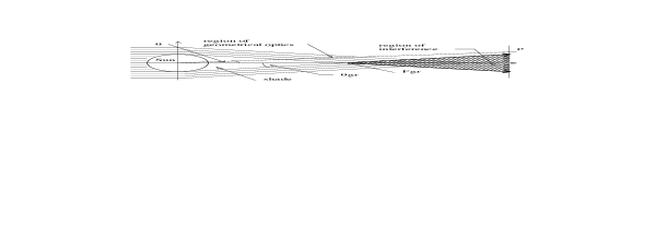
Figure 1: Different regions of the solar gravity lens.

By rigorously applying the methods of wave optics it was shown by Herlt and Stephani (1976) that the space behind the Sun may formally be separated into the three physically different regions, namely, (1) the shadow, (2) the region of geometric optics (where only one ray passes through each point of space), and (3) the region of interference (where two rays are passing through each point) as shown in Figure 1.

The solar shadowing effect prohibits focusing of light at distances shorter then ${\cal F}_{0}$ from the Sun. On the other hand, the most interesting effects, such as amplification of light, may only be observed in the third region – the region interference. Hence, in discussing the solar gravity lens, we shall be interested only in the solar region of interference. This region is defined to be at the distance ${\cal F}$ such as: ${\cal F}\geq{\cal F}_{0}$ and $\theta\leq|\theta_{0\,\tt gr}|$. This region may further be sub-divided onto several physically interesting regions. The most intriguing of those, is the region of extreme intensity, for which the following condition in the image plane (perpendicular to the optical axis) is satisfied: ${\lambda\over 2\pi}/{\sqrt{2r_{g}{\cal F}}}\ll\theta\ll\sqrt{{r_{g}/{\cal F}}}.$

For small departures $\rho$ of the observer from the optical axis $\rho\ll\sqrt{2r_{g}{\cal F}}$ solution may be obtained by the stationary phase method (see Herlt and Stephani (1976)) which yields the following expression for the gain $G(\rho,\lambda)$ of this lens:

$$G(\rho,\lambda)\cong 4\pi^{2}{r_{g}\over\lambda}J_{0}^{2}\left({2\pi\rho\over\lambda}\sqrt{{2r_{g}\over{\cal F}}}\right),$$ (3)

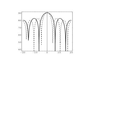
Off-set  distance,  $\rho$ [km]

Figure 2: Gain of the solar gravitational lens as seen in the image plane as a function of the optical distance ${\cal F}$ and possible observational wavelength $\lambda$. The dotted line represents gain for ${\cal F}=600~{}{\rm AU}$, the thick line is for ${\cal F}=1200~{}{\rm AU}$.

$J_{0}$ being a Bessel function of zero-order. The corresponding gain as a function of the optical distance and a possible observation wavelength is presented in Figure 2. Note that gain $G(\rho,\lambda)$ has it’s maximum on the axis

$$G_{\tt max}(0,\lambda)=4\pi^{2}{r_{g}\over\lambda}$$ (4)

for all points on the optical axis, the gain then decreases slowly (while oscillating) if $\rho$ increases (off-optical line), becoming

$$G(\rho_{1},\lambda)\cong\Big{(}{8\pi r_{g}\over\lambda}\Big{)}^{\frac{1}{2}}\qquad{\rm when}\qquad\rho_{1}=\Big{(}{\lambda{\cal F}\over\pi}\Big{)}^{\frac{1}{2}}$$ (5)

and going further down to its mean value $G=1$ for $\rho\gg\sqrt{{\cal F}\,r_{g}}$. Thus, as expected, the gravity lens is very sensitive to a tangential motions (e.q. in the image plane).

Another important feature of the solar gravity lens is a high angular resolution. To describe the angular resolution we will use the angle, $\epsilon_{10}$, that corresponds to the distance from the optical axis to the point where gain decreases by 10 dB:

$$\epsilon_{10dB}(b,\lambda)=\frac{\rho_{10dB}}{{\cal F}}\cong\frac{\lambda}{4\pi\sqrt{2r_{g}{\cal F}(b)}}=\frac{\lambda}{4\pi\sqrt{2r_{g}{\cal F}_{0}}}\Big{(}\frac{{\cal R}_{\odot}}{b}\Big{)}$$ (6)

where ${\rho_{10dB}}$ is the distance in the image plane where the gain decreases by 10 dB (the distance is given by $\rho_{10dB}\cong\frac{\lambda}{4\pi}\sqrt{\frac{{\cal F}}{2r_{g}}}$). For wavelength $\lambda\sim$ 1 mm resolution $\epsilon_{10}$ is estimated to be $\epsilon_{10dB}(b,1~{}{\rm mm})=0.11~{}{\cal R}_{\odot}/{b}~{}\pi{\rm rad}=0.11~{}\sqrt{{\cal F}_{0}/{\cal F}}~{}\pi$rad.

Since for the Sun the frequency can have values between $10^{4}$ Hz (radio waves) and $10^{10}$ Hz (visible light) or even $10^{14}$ Hz ($\gamma$-rays), a gravitational lens can enlarge the brightness of a star by the same remarkable factor. The plane wave is focused into a narrow beam of extreme intensity; the radius of which is $\rho=\sqrt{\lambda{\cal F}/\pi}$. The components of the Poynting vector and the intensity are oscillating with a spatial period

$$\delta\rho=\lambda\Big{(}{{\cal F}\over 8r_{g}}\Big{)}^{1\over 2}=1.18\times 10^{5}\Big{(}{\lambda b\over{\cal R}_{\odot}}\Big{)}.$$ (7)

Thus for $\lambda~{}\sim$ 1 mm this period is $\delta\rho=0.118\times b/{\cal R}_{\odot}$ km.

It is also useful to discuss the angular distribution of intensity. Thus, if telescope is small, the observed direction to the source will by determined by the corresponding deflection angle and the telescope’s position. However, if it is large, it will give a distribution of intensity ${\cal I}$ over the aperture

$${d{\cal I}\over d\theta}=\Big{(}{{\cal F}\over 2\rho}\Big{)}^{\frac{3}{2}}{\lambda\rho~{}d\theta d\phi\over\pi\sqrt{\theta}}$$ (8)

and the observer would essentially see a significantly magnified source at $\theta\cong 0$.

2.2 The effects of the solar atmosphere

The solar atmosphere introduces several complications to the above gravitational deflection scenario. They are due to the facts that it consists partly of a free-electron gas and that it is turbulent

2.2.1 Plasma frequency

First, a free electron gas responds to the (time) variable electric field of a passing electromagnetic wave and, for low enough frequencies, will absorb it. The plasma frequency, at which the refractive index of the plasma turns imaginary and hence absorptive, is proportional to the square-root of the electron density (e.g. Rubicki and Lightman (1979)) and therefore as we go progressively lower into the solar atmosphere, progressively higher frequencies of radio waves will not be able to propagate. Iess et al. (1999) have shown that the electron density at the Solar photosphere is of the order $(1-5)\times 10^{8}$ cm^-3. So, even for a quiet Sun, no radiation below a few hundred MHz can propagate through the solar atmosphere.

2.2.2 Refraction

Second, the density gradient in the solar atmosphere and hence the electron density influences the propagation of radio waves through the medium. Even for those frequencies which can propagate through it, the anisotropy of the solar atmosphere will cause refractive bending of the propagating rays. Since the density decreases outwards, this will cause a divergence in the propagating rays. Hence, the location of the focus for a given impact parameter will be shifted to larger distances than expected if the Sun did not have an atmosphere.

Any experiment involving propagation of an electromagnetic waves near the Sun faces a great challenge to overcome the refraction in the immediate solar vicinity due to various sources. The solar plasma is the main source of noise in an observations near the limb of the Sun. In general, one can express the total deflection angle $\theta_{\tt tot}$ as follows:

$$\theta_{\tt tot}=\theta_{\tt gr}+\theta_{\tt pl}+\theta_{\tt n},$$ (9)

where $\theta_{\tt pl}$ is the dominant plasma contribution, and $\theta_{\tt n}$ contains all non-dispersive sources of noise (pointing errors, attitude control, receiver, etc.), along with a minor dispersive contribution from the interstellar media, asteroid belt, and Kuiper belt, etc.

The plasma contribution $\theta_{\tt pl}$ to the total deflection angle is related to the change in the optical path

$$\Delta\ell={N_{e}(\ell)e^{2}\over 2\pi m_{e}\nu^{2}},$$ (10)

where $e$ is the electron’s charge, $m_{e}$ it’s mass, and $N_{e}(\ell)$ is the total columnar electron content along the beam, $N_{e}=\int n_{e}d\ell$. Therefore, in order to calibrate the plasma term, we should know the electron density along the path. We start by decomposing the electron density $n_{e}$ in static, spherically symmetric part $\overline{n}_{e}(r)$ plus a fluctuation $\delta n_{e}$, i.e.

$$n_{e}(t,{\bf r})=\overline{n}(r)+\delta n_{e}(t,{\bf r}).$$ (11)

The steady-state behavior is reasonably well known, and we can use one of the several plasma models found in the literature (Tyler et al., 1977; Muhleman, Esposito, and Anderson, 1977; Muhleman and Anderson, 1981). To be more explicit, we will refer to one particular model, namely (we do not consider here a correction factor due to the heliographic latitude):

$$\overline{n}_{e}(r)=\Big{[}\Big{(}{2.99\over\eta^{16}}+{1.55\over\eta^{6}}\Big{)}\times 10^{8}+{3.44\times 10^{5}\over\eta^{2}}\Big{]},~{}~{}{\rm cm}^{-3}$$ (12)

where $\eta=r/{\cal R}_{\odot}$. At large distances this model gives the expected behavior $\propto 1/r^{2}$ of the solar wind.

We will now determine the contribution to the total deflection angle due to the solar plasma for the model above. Following the usual method outlined in Iess et al. (1999), we obtain the corresponding deflection due to solar plasma $\theta_{\tt pl}$ as follows:

$$\theta_{\tt pl}(b,\nu)=\left({\nu_{0}\over\nu}\right)^{2}\left[~{}2.952\times 10^{3}\Big{(}{{\cal R}_{\odot}\over b}\Big{)}^{16}+2.28\times 10^{2}\Big{(}{{\cal R}_{\odot}\over b}\Big{)}^{6}+1.1\Big{(}{{\cal R}_{\odot}\over b}\Big{)}^{2}\right]$$ (13)

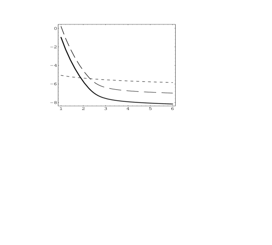
Impact  parameter,  $b~{}[{\cal R}_{\odot}]$

Figure 3: Refraction of radio-waves in the solar atmosphere. In this case we adopted the steady-state model, and considered X and K-bands radio frequencies (given by lowest dashed and thick lines correspondingly). The absolute value of the GR bending is also shown (dotted line).

with $\nu_{0}=6.32~{}{\rm MHz}$. Comparing $\theta_{\tt pl}$ with $\theta_{\tt gr}$ we notice the opposite sign - gravity bends the ray outwards, plasma inwards – and the different dependence on $b$, plasma being steeper. The plasma deflection as a function of the solar offset $b$ is shown in the Figure 3.

The presence of the solar atmosphere will result also in the de-focusing of the coherent radiation, thus worsening the quality of the solar gravitational lens. To analyze this influence let us estimate the optical distance for the two sources affecting the light propagation in the solar vicinity, namely gravity and plasma. One may expect that the beginning of the interference zone will be shifted further away from the Sun. For estimation purposes we will consider here only the steady-state part of the plasma model. The beginning of the interference zone (e.q. the effective optical distance) in this case may be determined from

$$\frac{b}{{\cal F}_{\tt gr+pl}}=\theta_{\tt tot}=\frac{2r_{g}}{b}-\theta_{\tt pl}.$$ (14)

This expression gives the effective optical distance for the system gravity+plasma ${\cal F}_{\tt gr+pl}\geq 0$:

$${\cal F}_{\tt gr+pl}(b,\nu)=546\,\Big{(}\frac{b}{{\cal R}_{\odot}}\Big{)}^{2}\Big{[}1-\frac{{\cal R}_{\odot}}{2r_{g}}\Big{(}\frac{b}{{\cal R}_{\odot}}\Big{)}\theta_{\tt pl}(b,\nu)\Big{]}^{-1}~{}~{}{\rm AU}$$ (15)

One may note that for any given impact parameter $b$ there is a critical frequency $\nu_{\tt crit}$ such that the denominator in the expression (15) vanishes and the effective optical distance ${\cal F}_{\tt gr+pl}$ becomes infinitive. This is the case when there is no lensing at all and the solar plasma entirely neutralizes influence of the solar gravity. This critical frequency is given as follows:

$$\nu^{2}_{\tt crit}(b)=\Big{(}2.161~{}{\rm GHz}\Big{)}^{2}\left[2.952\times 10^{3}\Big{(}{{\cal R}_{\odot}\over b}\Big{)}^{15}+2.28\times 10^{2}\Big{(}{{\cal R}_{\odot}\over b}\Big{)}^{5}+1.1\Big{(}{{\cal R}_{\odot}\over b}\Big{)}\right],$$ (16)

Based on the estimates for ${\cal F}_{\tt gr}$ presented in the Table 1 and from the practical considerations for the solar gravity lens mission, one will have to limit the range of possible impact parameters to those in the interval ${b}/{{\cal R}_{\odot}}\in[1.05,1.35]$, which correspond to the optical distance ${\cal F}_{\tt gr+pl}\in[601,1000[$ AU. For this range of impact parameter, the main contribution comes from the term $\sim\big{(}{{\cal R}_{\odot}/b}\big{)}^{15}$. Therefore, approximating to the sufficient order, we will have the critical frequency

$$\nu_{\tt crit}(b)=\nu_{0\,\tt crit}~{}\Big{(}{{\cal R}_{\odot}\over b}\Big{)}^{\frac{15}{2}},\qquad{b}/{{\cal R}_{\odot}}\in\Big{[}1.05,~{}1.35\Big{]}$$ (17)

with $\nu_{0\,\tt crit}\equiv\nu_{\tt crit}({\cal R}_{\odot})=120~{}{\rm GHz}$ or, equivalently, 2.5 mm. As a result of this analysis we find that the effective optical distance for the system gravity+plasma will be determined from the following expression:

$${\cal F}_{\tt gr+pl}(b,\nu)=546\,\Big{(}\frac{b}{{\cal R}_{\odot}}\Big{)}^{2}\Big{[}1-\frac{\nu^{2}_{0\,\tt crit}}{\nu^{2}}\Big{(}{{\cal R}_{\odot}\over b}\Big{)}^{15}\Big{]}^{-1}~{}~{}{\rm AU},\qquad{b}/{{\cal R}_{\odot}}\in\Big{[}1.05,~{}1.35\Big{]}$$ (18)

Results corresponding to a different frequencies are plotted in Figure 4. This represents the expected solar plasma response in this region of impact parameter $b\in[1.0-1.4]{{\cal R}_{\odot}}$. Note that only for the case when $\nu\gg\nu_{\tt crit}=120$ GHz is it possible to minimize the influence of the solar plasma and to allow for the geometric optics approximation to estimate the effects of solar microlensing (with some additional assumptions, for details see Herlt and Stephani (1976)). Hence, from this perspective the observational wavelength $\lambda$ for the chosen range of the impact parameters should be much smaller then $\lambda_{\tt crit}$.

It is worth noting that a solar plasma model similar to that given by Eq.(12) will be used for the Cassini relativity experiments at the solar conjunction. These experiments will utilize the dual frequency plasma cancellation technique with the telecommunication links available. For the 550 AU Mission the model for the solar plasma should be known to a highest degree accuracy including the latitude dependencies in the plasma distribution.

2.2.3 Turbulence

In the previous paragraph we have considered a spherical and static Solar atmosphere model, and derived the resulting plasma contribution to the total deflection angle. Unfortunately, the true electron density Eq. (9) contains also the fluctuations $\delta n_{e}$, which require particular attention. In fact, these fluctuations are carried along with the solar wind speed $V\approx 400$ km/s, so that their scale is $V\,\tau\approx{\cal R}_{\odot}/2$, where $\tau\approx 10^{3}$ s is the temporal scale. The solar atmosphere is highly variable over all time scales, due to solar activity; solar flares, coronal holes, solar rotation, etc. Moreover, on the typical scale of the gravitational deflection of light, one expects $\delta n_{e}$ to be of the same order of magnitude as its average (Armstrong, Woo, and Estabrook, 1979), i.e. $\delta n_{e}(t,b)\approx\langle n_{e}\rangle(b)$. In a conservative vein, it seems reasonable to assume that the deflection for an impact parameter $b$ is of the same order as the deflection for the mean solar atmosphere.

Two further physical optics effects come into play namely: spectral broadening and angular broadening, however, discussion of these effects is out of scope of present paper.

2.3 The Sun’s radiation

Because the Sun is a bright body and the observation of an object, gravitationally lensed by the sun necessitates pointings at, or close to the Sun itself, it will dominate the detector system at most wavelengths. Therefore, care has to be taken in selecting the optimum observing frequency and observing strategy. The integrated solar spectrum is well approximated by a 6000K black body for wavelengths below about 1cm. Longward of about 1cm the spectrum deviates from a blackbody and becomes dependent on the solar cycle. For the active Sun it rises to a secondary peak at around 1m. Therefore, a relative minimum exists just shortward of 1cm. However, even at 1mm the diffraction limited size of an antenna (of realistic size) will be large compared to the size of the solar disk. At 550 AU the sun subtends about 3.5” while a 10m antenna has a beam size of (FWFZ) about 50”. Hence, unless the source to be observed is strong, observations in the mm-wave range will have to be differential in wavelength space and have to require that the source has a different spectrum than the Sun. This observing strategy imposes severe requirements on the stability of the detector system, such that a reliable subtraction of the solar flux can be achieved. Coronografic observations can be envisioned at short (IR, visual) wavelength observations, however, in the IR and optical, emission and/or scattering from the Zodiacal dust will present a challenge for such observations. Further study is required to quantify these effects.

3 Observational considerations, Solar Gravitational Telescope

As noted above, in order to guarantee propagation of the radiation through the solar atmosphere, observations have to be restricted to frequencies above the plasma frequency at a given impact parameter as well as above those where the refraction cancels the gravitational convergence. If we want to minimize the distance from the Sun required this forces us to consider only frequencies well above about 100 GHz (3 mm).

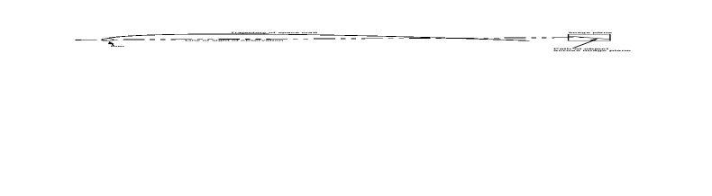
Figure 5: Conceptual sketch of a possible observing mode.

Both the magnification and the plate scale of a “Solar Gravitational Telescope” (SGT) - i.e. the tangential offset in the image plane corresponding to a given angular offset in the source - are very large. Since it is not possible, due to e.g. propulsion consideration to expect a solar gravitational lens mission to be able to perform much controlled tangential motion, the observational program has to be restricted to those that can be accomplished utilizing the trajectory given by the initial ejection from the inner solar system. This will first place very high requirements on the absolute navigation of the mission and in consequence the trajectory. Second, the source selection for a SGT is limited to sources that are small (because it takes a long time to transverse a source), but with interesting smaller-scale (of the order of the beam) variations which can be explored with one dimensional mapping. The source selection further has to be made prior to launch and hence survey-like observations are out of consideration. A likely observing scenario is thus to allow the tangential component of the trajectory velocity to sweep the space craft across the image of the source under study gathering a one dimensional map as illustrated in Figure 5. It is questionable whether any source can be found that both, can be successfully observed with a SGT and, cannot be observed better and cheaper using either ground based or Earth orbiting platforms.

4 Cruise Science

As with any mission aimed at reaching distances of several hundred AU a SGT mission can be used to carry out a wide range of in situ measurement while in cruise. Here we only briefly mention several possibilities. For a more detailed description the reader is referred to earlier studies (e.g. Etchegaray (1987)):

Heliospheric Science:

To date only a handful of missions have explored the outer reaches of the Heliosphere and none has passed beyond it. Collecting of in situ data on the density, flow and wave structures of the plasma as well as the magnetic field will help in our understanding of the solar wind and outer Heliosphere.

The termination of the Heliosphere:

The zone where the pressures of the Heliosphere and the local interstellar medium (LISM) come into balance is of great importance in understanding the interaction between the solar wind and the LISM as well as of the micro-physics of such interaction regions. Low frequency radio observations made by the Voyager 2 space craft now indicate that this transition region is located at about 85-150 AU in the upstream direction. By transversing the termination shock/heliopause/Bow shock region of the Heliosphere much can be learned about these processes.

LISM science:

Due to the shielding effect that the Heliosphere has on the particle fluxes in the ISM, little is known about the detailed density and composition of the LISM. Reaching outside of the Heliosphere will allow direct measurements of this region. What (e.g.) are the density fluctuations in the interstellar medium? What are the isotopic abundances in the LISM? The low energy end of the cosmic ray spectrum is heavily depleted as seen from Earth and is generally thought to be absorbed in the Heliosphere. However, in many processes in the interstellar medium, such as initiation of chemical reaction networks and heating of dense - starforming - gas, the exact form of this low energy spectrum is an important parameter. This spectrum could be measured once outside the heliopause.

Outer Solar system bodies:

If the appropriate telescopes and detectors are carried on the mission there is a, small, possibility of a chance encounter (within detection range) of bodies in the Kuiper belt or Oort cloud. This would (for Kuiper belt objects) require a trajectory in the ecliptic plane. However, as stated above, considerations directly related to the solar gravitational lensing suggests trajectories out of the ecliptic plane.

5 Conclusions

We have studied a few of the considerations required for a Solar gravitational lens mission. Specifically we have addressed a number of problems neglected by earlier studies of such a mission. The dominant effects neglected heretofore are those introduced by the plasma in the solar atmosphere. This plasma introduces absorption and scattering (systematic and random) of radiation propagating through it. The main effects are to limit the observable wavelength to those well above about 100 GHz and to increase the effective optical length of the SGT. We also note that given realistic constraints on the active control of the spacecraft trajectory a very limited class of sources can be targeted. The targets have to be small enough that interesting changes in their structure can be expected over several resolution elements ($\sim 10^{-7}$as) while bright enough to be observable very close to the solar disk. Major concerns regarding the achievability of the accuracy of the trajectory required to intercept the optical image of the object under study ($\sim 100~{}{\rm m}$) are raised.

Different regions of the solar gravity lens.

Gain of the solar gravitational lens as seen in the image plane as a function of the optical distance ${\cal F}$ and possible observational wavelength $\lambda$. The dotted line represents gain for ${\cal F}=600~{}{\rm AU}$, the thick line is for ${\cal F}=1200~{}{\rm AU}$.

Refraction of radio-waves in the solar atmosphere. In this case we adopted the steady-state model, and considered X and K-bands radio frequencies (given by lowest dashed and thick lines correspondingly). The absolute value of the GR bending is also shown (dotted line).

Effective optical distances for different frequencies and impact parameters. The upper curve corresponds to frequency of 170 GHz, then 300 GHz and 500 GHz, and at the bottom is for 1 THz.

Conceptual sketch of a possible observing mode.

Table 1: Estimates of the different terms influencing the effective optical distance. (Please refer to Eq.(16).)

${b}/{{\cal R}_{\odot}}$	${\cal F}_{\tt gr}$, AU	$\sim\Big{(}{{\cal R}_{\odot}/b}\Big{)}^{15}$	$\sim\Big{(}{{\cal R}_{\odot}/b}\Big{)}^{5}$	$\sim\Big{(}{{\cal R}_{\odot}/b}\Big{)}$
1	546	2952	228	1.1
1.05	601	1426	178	1
1.1	660	704	141	1
1.15	722	364	113	0.96
1.2	785	192	92	0.92
1.25	853	104	75	0.88
1.3	922	58	62	0.85
1.35	996	32	51	0.81
1.4	1070	19	43	0.78
1.5	1228	7	30	0.73
1.6	1397	2	22	0.69

$\lambda=1~{}{\rm mm}$

Off-set  distance,  $\rho$ [km]

Gain,  $G({\cal F},\lambda)$  [dB]

Gain,  $G({\cal F},\lambda)$  [dB]

$\lambda=0.1~{}{\rm mm}$

Refraction  angle,  ${\rm log}_{10}\theta_{\tt pl}(b,\nu)$  [rad]

Effective  distance,  ${\cal F}_{\tt gr+pl}(b,\nu)~{}[{\rm AU}]$

Impact  parameter,  $b~{}[{\cal R}_{\odot}]$

Figure 4: Effective optical distances for different frequencies and impact parameters. The upper curve corresponds to frequency of 170 GHz, then 300 GHz and 500 GHz, and at the bottom is for 1 THz.

References

- Armstrong, Woo, and Estabrook (1979) Armstrong, J.W., Woo, R. & Estabrook, F.B. 1979, ApJ, 203, 570
- Blandford and Narayan (1992) Blandford, R.D. & Narayan, R. 1992, ARA&A, 30, 311
- Bliokh and Minakov (1975) Bliokh, P.V. & Minakov, A.A. 1975, Ap&SS, 34, L7
- Eddington (1919) Eddington, A.S. 1919, Observatory 42, 119
- Etchegaray (1987) Etchegaray, M.I. 1987, JPL Publications, 87-17
- Heidmann and Maccone (1994) Heidmann, J. & Maccone, C. 1994, Acta Astronautica, 32, 409
- Herlt and Stephani (1976) Herlt, E. & Stephani, H. 1976, International Journal of Theoretical Physics, 15(1), 45
- Iess et al. (1999) Iess, L., Giampieri, G., Anderson, J.D., and Bertotti, B. 1999, Class. Quant. Grav. 16, 1487
- Kraus (1986) Kraus, J.D. 1986, Radio Astronomy, p.6-115
- Muhleman, Esposito, and Anderson (1977) Muhleman, D.O., Esposito, P.B. & Anderson, J.D. 1977, ApJ, 211, 943
- Muhleman and Anderson (1981) Muhleman, D.O. & Anderson, J.D. 1981, ApJ, 247, 1093
- Paczynski (1996) Paczynski, B. 1996, ARA&A, 34, 419
- Refsdal (1965) Refsdal, S. 1965, In Proc. of Conference on General Relativity and Gravitation, London
- Rubicki and Lightman (1979) Rubicki, G.P. & Lightman, A.P. 1979, “Radiative Processes in Astrophysics”, p. 226, Wiley, New York
- Tyler et al. (1977) Tyler, G.L., Brenkle, J.P., Komarek, T.A. & Zygielbaum, A.I. 1977, J. Geophys. Res., 82, 4335
- von Eshleman (1979) von Eshleman, R. 1979, Science, 205, 1133