Abstract

An example illustrating a continuum spin foam framework is presented. This covariant framework induces the kinematics of canonical loop quantization, and its dynamics is generated by a renormalized sum over colored polyhedra.

Physically the example corresponds to $3$d gravity with cosmological constant. Starting from a kinematical structure that accommodates local degrees of freedom and does not involve the choice of any background structure (e. g. triangulation), the dynamics reduces the field theory to have only global degrees of freedom. The result is projectively equivalent to the Turaev-Viro model.

I. INTRODUCTION

Several TQFT’s can be written as a sum over assignments of spins to polyhedra: that is, as spin foam models. A trend in today’s research is to try to find a model of a similar type that is related to $4$d gravity [1]. Regarding these models as fundamental amounts to postulating that gravity is only effectively a field theory, but fundamentally it has only finitely many degrees of freedom and a privileged polyhedron (or triangulation) comes along with spacetime. It has been proposed to get rid of this extra structure with a sum over triangulations [2]. In this article we will explore another route. We will regard the continuum as fundamental and take the diffeomorphism invariance of general relativity as the guiding symmetry. We share this principle with canonical loop quantization [3].

In this paper we present an example. It is defined in the continuum, but it turns out to be equivalent to the Turaev-Viro model [4]. The interest of our example relies on the fact that it is a continuum spin foam model. More precisely, the construction induces the kinematics of q-deformed loop quantization in the spatial slices, and the projector to the space of physical states is constructed as a renormalized sum over colored (by spins) polyhedra.

The construction does not involve the choice of any background structure, and the diffeomorphism group acts faithfully at the kinematical level.

The strategy used to generate this family of examples (one for every value of a deformation parameter) can be adapted to other spin foam models. A “renormalizability condition” determines whether the continuum theory exists. The proof that other topological models satisfy the condition proceeds almost in complete parallel to the proof given here. Interestingly, there are reasons to believe that there are other examples corresponding to genuine field theories. In the case of compact QED, the first steps in this direction have already been taken [5].

In section II we construct the example and prove the equivalence with the Turaev-Viro model. Section III gives an interpretation of the projector as a renormalized sum over quantum geometries.

II. A CONTINUUM SPIN FOAM MODEL

This is the central section of the paper. In the beginning we present the construction of the example and show its main properties. With minor modification of the proofs, the construction applies to other topological spin foam models and the same strategy could apply to other less trivial spin foam models as well. In the last subsection, we prove the projective equivalence with the Turaev-Viro model.

A. Embedded graphs and embedded polyhedra

In this work all the spaces and maps are piecewise linear.

Consider a compact surface without boundary $\Sigma$. By an embedded graph $\Gamma$ we mean a finite one-dimensional $CW$-complex all whose vertices have valence two or bigger, together with an embedding into $\Sigma$. The set of all graphs embedded into a given surface will be denoted by $G(\Sigma)$. This set has a natural partial order given by inclusion and it is directed.

Similarly, consider a $3$-manifold with boundary $M$. By an embedded polyhedron $X$ we mean a finite two-dimensional $CW$-complex all whose internal edges have valence two or bigger, together with an embedding into $M$ such that $X\cap\partial M$ denoted by $\partial X$ belongs to $G(\partial M)$. The set of all polyhedra embedded into a given $3$-manifold will be denoted by $P(M)$. Again, this set is partially ordered and directed.

B. Data from lattice gauge theory

Our construction starts with data generated by “lattice gauge theory” on all lattices embedded into given spacetimes.

For every $\Gamma\in G(\Sigma)$ we are given a complex vector space $C(\Gamma)$ and for every $X\in P(M)$ we are given a linear functional $\Omega^{n}_{X}:C(\partial X)\to{\rm\bf C}$. Thus, for each surface $\Sigma$ we get a collection of vector spaces labeled by embedded graphs and for each $3$-manifold $M$ we get a collection of linear functionals labeled by embedded polyhedra. Our work is based on the compatibility of these collections of structures with the partial order of the labeling sets.

Now we define these objects in the example presented here. We follow the notation of Turaev and Viro [4] as closely as possible as well as their conventions and normalizations.

Fix an integer $r\geq 3$ and denote by $I$ the set of spins $\{0,1/2,\ldots,(r-2)/2\}$. A triple of spins is admissible, $(i,j,k)\in adm$, if $i+j+k$ is an integer and

$$i\leq j+k,\quad j\leq k+i,\quad k\leq i+j,\quad i+j+k\leq r-2.$$

Given an embedded graph $\Gamma\in G(\Sigma)$ we assign to it an abstract simple graph $\Gamma_{s}$. The vertices of a simple graph are always trivalent; a graph dual to a triangulation is an example of a simple graph.

$\Gamma_{s}$ is constructed by blowing up the vertices of $\Gamma$ as we explain below. To each edge of $\Gamma$ corresponds one edge in $\Gamma_{s}$ and to each vertex of $\Gamma$ we assign several “internal vertices” and “internal edges” in $\Gamma_{s}$ in the manner indicated by Figure 1.

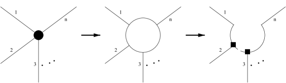
Figure 1: The construction uses an arbitrary numbering of the edges coming to a vertex. Internal vertices are shown as square dots and internal edges are dashed lines.

A coloring $\alpha$ of $\Gamma$ is an assignment of spins to its edges and intertwiners to its vertices. An intertwiner is a coloring (with spins) of the internal edges assigned to the vertex. Clearly, a coloring $\alpha$ of $\Gamma$ induces a coloring of $\Gamma_{s}$, an assignment of spins to its edges. The coloring is admissible, $\alpha\in adm(\Gamma)$, if at each vertex $v$ of $\Gamma_{s}$ the triple $(\alpha(e_{1}(v)),\alpha(e_{2}(v)),\alpha(e_{3}(v)))\in adm$.

Then $C(\Gamma)$ is defined by

$$C(\Gamma)={\mathbb{C}}[adm(\Gamma)]$$

where ${\mathbb{C}}[adm(\Gamma)]$ is the complex vector space freely generated by the elements of $adm(\Gamma)$; in addition, the inner product makes $adm(\Gamma)$ an orthonormal set. A different choice of internal structure in the construction of $\Gamma_{s}$ results in an a priori different vector space; however “recoupling moves” on the internal edges define an isomorphism between any two spaces generated by different choices. This is reviewed in the Appendix. We identify all these isomorphic vector spaces and call them $C(\Gamma)$.

In the non q-deformed case, when the set of spins is infinite, the space just constructed is the space of square integrable functions of (generalized) $SU(2)$-connections [6], and it is the heart of the kinematics of canonical loop quantum gravity [3].

$X_{s}$, a simple abstract polyhedron, is constructed by blowing up the edges and vertices of $X\in P(M)$ as we explain below. We proceed in complete parallel to the case of graphs. First, we surround every edge by a cylindrical neighborhood and every vertex by a spherical neighborhood; in this way we created an internal (empty) bubble for each edge and vertex of $X$ in analogy with the middle picture of Figure 1. Then, we will erase one internal face in each internal bubble, as we did in the last picture of Figure 1, to create $X_{s}$. There are only two rules to select the face to be erased from each internal bubble. In the case of edge-bubbles, we erase one of the lateral faces (not a face shared with a vertex-bubble). And in the case of the vertex-bubbles, we erase one of the faces shared with an edge-bubble. Notice that the valence of any edge in $X_{s}$ is three and that at every vertex of $X_{s}$ six faces meet.

A coloring $\varphi$ of $X$ is an assignment of spins to its faces and intertwiners to its edges. An intertwiner is a coloring (with spins) of the internal faces assigned to the edge. The coloring is admissible, $\varphi\in adm(X)$, if at each edge $e$ of $X_{s}$ the triple $(\varphi(f_{1}(e)),\varphi(f_{2}(e)),\varphi(f_{3}(e)))\in adm$.

Each colored polyhedra is assigned a weight. This assignment is a simple extension of the Turaev and Viro weight to embedded (not necessarily simple) polyhedra. The Turaev-Viro weight is constructed as the product of weights assigned to its vertices and faces (with a correction due to the boundary edges) [4].

$$|X|_{\varphi}=|X_{s}|^{TV}_{\varphi}=w^{-2\chi(X_{s})+\chi(\partial X_{s})}\prod_{f\in F(X_{s})}w_{\varphi(f)}^{2\chi(f)}\prod_{e\in E(X_{s})}w_{\partial\varphi(e)}^{\chi(e)}\prod_{v\in V(X_{s})}|\hat{T}_{v}|_{\varphi}$$

Here $\chi$ denotes Euler characteristic. $w_{\varphi(f)}$ and $w_{\partial\varphi(e)}$ denote the quantum group analog of the dimension of the spin $j$ representation for $j=\varphi(f)$ and $j=\partial\varphi(e)$ respectively. $|\hat{T}_{v}|_{\varphi}$ is the quantum $6j$ symbol corresponding to the $6$-tuple of spins of the faces meeting at vertex $v$.

Then $\Omega_{X}:C(\partial(X))\to{\mathbb{C}}$ is defined by $\Omega_{X}(\alpha)=\sum_{\varphi}|X|_{\varphi}$, where the sum runs over the colorings $\varphi\in adm(X)$ that induce $\alpha$ in the boundary. We will work with the linear functional normalized dividing by the “vacuum to vacuum amplitude” $\Omega_{X}(j=0)$,

$$\Omega^{n}_{X}(\alpha)=\frac{\Omega_{X}(\alpha)}{\Omega_{X}(j=0)}.$$

Note that $\Omega^{n}_{X}(\alpha)$ can also be defined from $\Omega^{\prime}_{X}(\alpha)=\sum_{\varphi}|X|^{\prime}_{\varphi}$ which is defined from a less refined Turaev-Viro weight $|X|^{\prime}_{\varphi}$ in which the normalizing factor $w^{-2\chi(X_{s})+\chi(\partial X)}$ is omitted.

The construction of $X_{s}$ involves a choice of “internal structure” on the edges of $X$. However, the invariance results of Turaev and Viro imply that $\Omega_{X}$ and $\Omega^{\prime}_{X}$ are independent of this choice. This is reviewed in the Appendix.

The weight assigned to a colored polyhedron is what defines the dynamics of this example. We extended the Turaev-Viro weight in a simple manner, but it is possible to derive a weight assignment for general polyhedra that reduces to the Turaev-Viro weight in the case of simple polyhedra [7].

C. From lattices to the continuum

Now we will leave single “lattices” and go to the continuum.

Consider two embedded graphs $\Gamma_{1}\leq\Gamma_{2}$ in $G(\Sigma)$. It is easy to see that $\alpha\in adm(\Gamma_{1})$ defines an admissible coloring in $\Gamma_{2}$ by simply extending the coloring with color $j=0$ in the additional edges and extending the intertwiners also coloring with $j=0$ in the additional internal edges. Thus, we can take this natural inclusion for granted and write $C(\Gamma_{1})\subset C(\Gamma_{2})$. Due to this property we can define $C(\Sigma)$ as the inductive limit or co-limit [9] of the nested spaces labeled by graphs,

$$C(\Sigma)=\hbox{co-}\!\!\lim_{\Gamma\to\Sigma}C(\Gamma).$$

Similarly, for $\alpha\in C(\partial M)$ induced by $\alpha\in adm(\Gamma)$ we define

$$\Omega^{n}_{M}(\alpha)=\lim_{X\to M}\Omega^{n}_{X}(\alpha),\quad\partial X\geq\Gamma.$$ (1)

When the limit exists it defines $\Omega^{n}_{M}:C(\partial M)\to C$. In our example we prove its existence in the next subsection. However, the analogous limit in theories constructed from other lattice gauge theories may not exist. The existence of the limit should be interpreted as a renormalizability condition.

Note that the extendibility of colorings from subgraphs implies that $adm(\Sigma)$ and similarly $adm(M)$ can be defined. A coloring in $\alpha\in adm(\Sigma)$ should be thought of as a coloring of all graphs, bigger than a certain minimal graph $\Gamma(\alpha)$, that is compatible with inclusion of graphs. We then have the equivalent definition $C(\Sigma)={\mathbb{C}}[adm(\Sigma)]$.

D. Renormalizability and cellular decompositions

A polyhedron $X\in M$ induces a cellular decomposition for $(M,\Gamma)$, where $\Gamma\in G(\partial M)$, if $\partial X=\Gamma$ and $M-\partial M-X$ is a disjoint union of open balls.

Theorem 1

Given any polyhedron $X\in P(M)$ there is a finer polyhedron $X^{\prime}\in P(M)$, $X\leq X^{\prime}$, such that $X^{\prime}$ induces a cellular decomposition for $(M,\Gamma)$ for some $\Gamma\geq\partial X$.

Proof. First note that for every manifold with boundary one can find embedded polyhedra inducing cellular decompositions. Take for example the cellular complex dual to any triangulation of the manifold. Once we have one cellular decomposition, we can generate many by subdivision of the induced cells adding faces to the original polyhedron.

Let $X^{\prime\prime}\in P(M)$ induce a cellular decomposition that is sufficiently fine in the sense that for each open ball in $\cup_{r=1}^{n}B_{r}=M-\partial M-X^{\prime\prime}$ we have that $B_{r}-X$ is a finite union of open balls, $B_{r}-X=\cup_{s=1}^{m}{}_{r}B^{\prime}_{r,s}$.

Since we are working with piecewise-linear spaces, such a $X^{\prime\prime}$ can be constructed from an initial cellular decomposition after finitely many refinements.

Let $X^{\prime}=X^{\prime\prime}\cup X$. Then $M-\partial M-X^{\prime}=\cup_{r=1}^{n}\cup_{s=1}^{m}{}_{r}B^{\prime}_{r,s}$. $\Box$

Theorem 2

Fix $X\in P(M)$ a polyhedron inducing a cellular decomposition of $(M,\Gamma)$. For any finer polyhedron $X^{\prime}\in P(M)$, $X\leq X^{\prime}$, we have

$$\Omega^{n}_{X}=\Omega^{n}_{X^{\prime}}|_{C(\partial X)}.$$

The proof of this theorem requires some previous definitions and lemmas presented after the following corollary.

Corollary 1 (Renormalizability)

In the definition

$$\Omega^{n}_{M}=\lim_{X\to M}\Omega^{n}_{X}$$

the limit exists. In this sense, the theory defined by the collection of linear functionals $\Omega^{\prime}_{X}$ is renormalizable.

We should mention that for the linear functionals $\Omega^{\prime}_{X}$ and $\Omega_{X}$ the limit does not exist. Only the renormalized functional exists in the continuum.

Wedge and corner moves generalize the lune $\cal{L}$ and Matveev $\cal{M}$ moves (and their inverses) on simple polyhedra. Wedge moves describe a face of an embedded polyhedron $X\in P(M)$ sliding through a wedge, while in corner moves a face slides through a corner. See Figure 2.

Figure 2: In each picture the paper corresponds to a set of faces of a portion of the polyhedron. The solid lines indicate edges where one (or more) faces meet the paper from above. The dashed lines correspond to faces that are below the paper. (a) Illustrates a top face(s) sliding through a wedge with bottom face(s). (b) Illustrates a top face(s) sliding through a corner with bottom faces.

Lemma 1 (Invariance under wedge and corner moves)

Let $X\in P(M)$ and $\alpha\in adm(\partial X)$. Then $\Omega^{\prime}_{X}(\alpha)$ is invariant under wedge and corner moves.

Proof. It is clear that a wedge move in $X$ induces a sequence of ${\cal{L}}$ or ${\cal{L}}^{-1}$ moves in $X_{s}$. Similarly, a corner move in $X$ induces a sequence of ${\cal{M}}$ and/or ${\cal{M}}^{-1}$ and/or ${\cal{L}}$ and/or ${\cal{L}}^{-1}$ in $X_{s}$. Thus, this lemma is a direct consequence of the similar invariance lemmas of Turaev and Viro [4]. $\Box$

The following lemma is a well-known consequence of the definition a properties of $|X|^{\prime}_{\varphi}$; see [4, 8].

Lemma 2 (The color $j=0$ is invisible)

Let $X\in P(M)$ and $\varphi\in adm(X)$. Construct the polyhedron $X(\varphi)$ erasing from $X$ the “invisible” $2$-strata, the ones colored with $j=0$. Then

$$|X(\varphi)|^{\prime}_{\varphi}=|X|^{\prime}_{\varphi}.$$

Also, for $\alpha\in adm(\partial X)$ construct $X(\alpha)$ erasing from $X$ the $2$-strata meeting $\partial X$ in edges colored with $j=0$. Then

$$\Omega^{\prime}_{X(\alpha)}(\alpha)=\Omega^{\prime}_{X}(\alpha).$$

Proof of Theorem 2. Consider a collection of nested polyhedra $\{X_{r}\}$ such that $X=X_{1}\leq X_{2}\leq\ldots\leq X_{n}=X^{\prime}$ where $X_{r+1}-X_{r}\subset B_{s(r)}$ for some cell $B_{s}$ in $\cup_{s=1}^{n}B_{s}=M-\partial M-X$ with $B_{s(r)}\not=B_{s(t)}$ if $r\not=t$.

We will show that $\Omega^{n}_{X_{r+1}}|_{C(\partial X_{r})}=\Omega^{n}_{X_{r}}$.

Let $\partial B_{s(r)}-\partial M=\cup_{u=1}^{m}F_{u}$ with $F_{u}$ faces of $X$.

The closures of the faces in $X_{r+1}-X_{r}$ may intersect several of the faces of $\partial B_{s(r)}$, but we can use wedge and corner moves on $X_{r+1}$ (inside $B_{s(r)}$) until only $F_{1}$ (and $\partial M$ if $B_{s(r)}$ is a boundary cell) is intersected. Call the resulting polyhedron $Y^{\prime}_{r+1}$. Remove from $Y^{\prime}_{r+1}$ the $2$-strata meeting $\partial Y^{\prime}_{r+1}-\partial X_{r}$; we call this polyhedron $Y_{r+1}$.

Let $B\subset M$ be an open ball such that $Y_{r+1}-X_{r}\subset B$, and $B\cap X_{r}$ lies in the interior of $F_{1}$.

Then

$$\Omega^{\prime}_{X_{r+1}}|_{C(\partial X_{r})}(\alpha) = \Omega^{\prime}_{Y_{r+1}}(\alpha)=\sum_{\beta\in adm(Y_{r+1}\cap\partial B)}\Omega^{\prime}_{Y_{r+1}\cap B^{c}}(\alpha\cup\beta)\Omega^{\prime}_{Y_{r+1}\cap\bar{B}}(\beta)$$

$$= \sum_{\beta\in adm(X_{r}\cap\partial B)}\Omega^{\prime}_{X_{r}\cap B^{c}}(\alpha\cup\beta)\Omega^{\prime}_{Y_{r+1}\cap\bar{B}}(\beta)$$

$$= \lambda\sum_{\beta\in adm(X_{r}\cap\partial B)}\Omega^{\prime}_{X_{r}\cap B^{c}}(\alpha\cup\beta)\Omega^{\prime}_{X_{r}\cap\bar{B}}(\beta)=\lambda\Omega^{\prime}_{X_{r}}(\alpha)$$

where $B^{c}$ and $\bar{B}$ denote the complement and the closure of $B$ respectively. In the first equality Lemma 1 and Lemma 2 were used. In the second and fifth equalities the associativity of $\Omega^{\prime}$ was used. The fourth equality is due to the following lemma.

Lemma 3

The quotient $\frac{\Omega^{\prime}_{Y_{r+1}\cap\bar{B}}(\beta)}{\Omega^{\prime}_{X_{r}\cap\bar{B}}(\beta)}=\lambda$ is independent of the coloring.

Proof of the Lemma. Let $(\beta,\alpha,k)\in adm$. The proof follows picture in Figure 3.

Figure 3: The pictures should be thought of as $\Omega^{\prime}$ evaluations with the indicated boundary coloring.

In the upper left picture the face with a circle and an $X$ inside represents $Y_{r+1}\cap\bar{B}$; the rest of the faces play only an auxiliary role. Using wedge moves the $X$ slides through the edge. The result is the picture in the bottom left. There we can again identify the face with a circle and an $X$ with $Y_{r+1}\cap\bar{B}$. From the pictures in the left to the ones in the right we have only used $\Omega^{\prime}_{Y_{r+1}\cap\bar{B}}(\gamma)=\lambda(\gamma)\Omega^{\prime}_{X_{r}\cap\bar{B}}(\gamma)$.

The lemma follows from the fact that the set of spins is $adm$-connected; given any two spins there is a chain of admissible triples linking them. $\Box$

This completes the proof of Theorem 2. $\Box$

E. Spaces of physical states and propagators

We will now define adequate spaces of physical states and propagators. To do this cleanly we need to use the language of cobordism theory. A cobordism $W$ is defined by the triple $W=(M;i_{\Sigma_{0}}:\Sigma_{0}\to\partial M,i_{\Sigma_{1}}:\Sigma_{1}\to\partial M)$ where $M$ is a $3$-manifold with boundary, $\Sigma_{0}$ and $\Sigma_{1}$ are compact surfaces without boundary, $\partial M=i_{\Sigma_{0}}(\Sigma_{0})\cup i_{\Sigma_{1}}(\Sigma_{1})$ and $i_{\Sigma_{0}}(\Sigma_{0})\cap i_{\Sigma_{1}}(\Sigma_{1})=\emptyset$. Cobordisms can be composed in an obvious way. Also, there is a special cobordism for each $\Sigma$ compact surface without boundary, $id_{\Sigma}=(\Sigma\times I;i_{0}(p)=(p,0),i_{1}(p)=(p,1))$.

To every $\Sigma$ we assign a space of physical states $H(\Sigma)\subset C(\Sigma)^{*}$ defined by $H(\Sigma)=\Omega^{n}_{\Sigma\times I}(C(\Sigma))$. In the jargon of the field $\Omega^{n}_{\Sigma\times I}$ is referred to as the “generalized projector,” even though $H(\Sigma)\subset C(\Sigma)^{*}$. It is useful to note that $H(\Sigma)$ is spanned by vectors $\bar{\alpha}$ defined by

$$\bar{\alpha}[\delta]=\Omega^{n}_{\Sigma\times I}(i_{0}^{-1*}\alpha\cup i_{1}^{-1*}\delta)$$

where $\alpha,\delta\in C(\Sigma)$ and we have used the pull back maps $i_{0}^{-1*}:adm(\Sigma)\to adm(\partial(\Sigma\times I)_{t=0})$, $i_{1}^{-1*}:adm(\Sigma)\to adm(\partial(\Sigma\times I)_{t=1})$. The inner product in $H(\Sigma)$ is defined by

$$(\bar{\alpha},\bar{\beta})=\bar{\alpha}(\beta).$$

Now for a general cobordism define the map $\Phi^{n}_{W}:H(\Sigma_{0})\to C(\Sigma_{1})^{*}$ by

$$\Phi^{n}_{W}(\bar{\alpha})[\delta]=\Omega^{n}_{M}(i_{0}^{-1*}\alpha\cup i_{1}^{-1*}\delta).$$

Theorem 3

$\Phi^{n}_{W}(H(\Sigma_{0}))\subset H(\Sigma_{1})$

Proof. Consider a regular neighborhood $M^{\prime\prime}$ of $i_{\Sigma_{1}}\Sigma_{1}$ in $M$; it has the $\Sigma_{1}\times I$ topology. Denote its boundary by $\partial M^{\prime\prime}=\Sigma^{\prime}_{1}\cup\Sigma_{1}$. Also call $M^{\prime}=M-M^{\prime\prime}$; clearly $M^{\prime}\approx M$ and $\partial M^{\prime\prime}=\Sigma_{0}\cup\Sigma^{\prime}_{1}$.

We are gong to compute $\Phi^{n}_{W}(\bar{\alpha})[\delta]$ using the following auxiliary structures: First, two boundary graphs $\Gamma_{0},\Gamma_{1}$ such that $\Gamma_{0}\geq\Gamma(\alpha)$ and $\Gamma_{1}\geq\Gamma(\delta)$. Second, $X\in P(M)$ inducing a cellular decomposition of $(M;i_{\Sigma_{0}}\Gamma_{0}\cup i_{\Sigma_{1}}\Gamma_{1})$ such that $X|_{M^{\prime\prime}}\in P(M^{\prime\prime})$ induces a cellular decomposition of $(M^{\prime\prime};i_{\Sigma_{0}}\Gamma_{0}\cup i_{\Sigma^{\prime}_{1}}\Gamma^{\prime}_{1})$, and $X|_{M^{\prime}}\in P(M^{\prime})$ induces a cellular decomposition of $(M^{\prime};i_{\Sigma^{\prime}_{1}}\Gamma^{\prime}_{1}\cup i_{\Sigma_{1}}\Gamma_{1})$.

$$\Phi^{n}_{W}(\bar{\alpha})[\delta] = \frac{\Omega^{\prime}_{X}(\alpha\cup\delta)}{\Omega^{\prime}_{X}(j=0)}=\sum_{\beta}\frac{\Omega^{\prime}_{X|_{M^{\prime}}}(\alpha\cup\beta)\Omega^{\prime}_{X|_{M^{\prime\prime}}}(\beta\cup\delta)}{\Omega^{\prime}_{X}(j=0)}$$ (2)

$$= (\frac{\Omega^{\prime}_{X|_{M^{\prime}}}(j=0)\Omega^{\prime}_{X|_{M^{\prime\prime}}}(j=0)}{\Omega^{\prime}_{X}(j=0)})\sum_{\beta}\Omega^{n}_{M^{\prime}}(i_{\Sigma_{0}}^{-1*}\alpha\cup i_{\Sigma^{\prime}_{1}}^{-1*}\beta)\Omega^{n}_{M^{\prime\prime}}(i_{\Sigma^{\prime}_{1}}^{-1*}\beta\cup i_{\Sigma_{1}}^{-1*}\delta)$$

$$= \lambda(\Gamma^{\prime}_{1})\sum_{\beta}\Omega^{n}_{M}(i_{\Sigma_{0}}^{-1*}\alpha\cup i_{\Sigma_{1}}^{-1*}\beta)\Omega^{n}_{\Sigma\times I}(i_{0}^{-1*}\beta\cup i_{1}^{-1*}\delta)$$

The sums are over $\beta\in adm(\Gamma^{\prime}_{1})$. In the last equality we used the invariance under homeomorphisms; this property follows from the definitions and will be described in the next subsection. We could have used another cellular decomposition to perform the calculation or another auxiliary surface $\Sigma^{\prime}_{1}$. The result would have been another expression for the same element of $H(\Sigma)$.

The desired result follows from the above equation. $\Box$

Note that the maps assigned to identity cobordisms are identity maps, $\Phi^{n}_{id_{\Sigma}}|_{H(\Sigma)}=id_{H(\Sigma)}$. Now we show that $\Phi^{n}_{W}$ satisfies the projectivized propagator condition.

Theorem 4

For any two composable cobordisms, $W_{1}=(M_{1};i_{\Sigma_{0}},i_{\Sigma_{1}})$ and $W_{2}=(M_{2};i^{\prime}_{\Sigma_{1}},i_{\Sigma_{2}})$, we have $\Phi^{n}_{W_{2}}\circ\Phi^{n}_{W_{1}}=\lambda\Phi^{n}_{W_{2}\circ W_{1}}$ .

Proof. The definition of $\Phi^{n}_{W}$ requires that its argument is written in a canonical form. We use (2). We follow the strategy of the previous theorem’s proof: with $X$ an auxiliary polyhedron giving a cellular decomposition for $W_{1}$ and $Y$ for $W_{2}$, we will write the expression in terms of $\Omega^{\prime}$ to use associativity. Then we will rewrite in terms of the renormalized objects of $X\cup Y$, which is an auxiliary polyhedron giving a cellular decomposition for $W_{2}\circ W_{1}$.

$$\Phi^{n}_{W_{2}}\circ\Phi^{n}_{W_{1}}(\bar{\alpha})(\delta) = \lambda(\Gamma^{\prime}_{1})\sum_{\beta}\Omega^{n}_{M_{1}}(i_{\Sigma_{0}}^{-1*}\alpha\cup i_{\Sigma_{1}}^{-1*}\beta)\Omega^{n}_{M_{2}}({i^{\prime}}_{\Sigma_{1}}^{-1*}\beta\cup i_{\Sigma_{2}}^{-1*}\delta)$$

$$= \lambda(\Gamma^{\prime}_{1})(\frac{\Omega^{\prime}_{X\cup Y}(j=0)}{\Omega^{\prime}_{X}(j=0)\Omega^{\prime}_{Y}(j=0)})\Omega^{n}_{X\cup Y}(\alpha\cup\delta)$$

$$= \lambda(\Gamma^{\prime}_{1})\Lambda(\Gamma_{1})\Phi^{n}_{W_{2}\circ W_{1}}(\bar{\alpha})(\delta)\qquad\Box$$

Here we proved the last two theorems for the example that we are presenting, but the proofs extend with very little change to the general case in which the renormalizability condition (1) holds.

F. Action of the homeomorphism group

A homeomorphism between two manifolds with boundary $f:M\to N$ induces a map among the spaces of embedded polyhedra. Colorings are pulled back by this map. Similarly, the restriction of the map to the boundaries induces a pull back map among the spaces of colorings which leads to $U_{f}:C(\partial M)\to C(\partial N)$ defined by the action $U_{f}(\alpha)=f^{-1*}(\alpha)$. The following identities describe the action of homeomorphisms

$$|X|^{\prime}_{\varphi}=|f(X)|^{\prime}_{f^{-1*}\varphi},\quad\Omega^{\prime}_{X}(\alpha)=\Omega^{\prime}_{f(X)}(f^{-1*}\alpha),\quad\Omega^{n}_{M}=\Omega^{n}_{f(M)}\circ U_{f}.$$

Note that the action of $f$ is not trivial due to its action in the boundaries. The language of the last subsection already assumes this level of invariance; $W$ is only sensible to $M$ up to a homeomorphism preserving the boundary. By dual action of $U_{f}$ we have a representation of the modular group (mapping class group) of $\Sigma$ on $H(\Sigma)$. Indeed, if $f$ and $g$ are two isotopic homeomorphisms, $U_{f}$ and $U_{g}$ induce the same map in $H(\Sigma)$. In particular, if $f$ is connected to the identity

$$U_{f}|_{H(\Sigma)}=id_{H(\Sigma)}.$$

Thus, for homeomorphisms connected with the identity we have $\Omega^{n}_{f(M)}=\Omega^{n}_{M}$.

In relation with canonical loop quantum gravity we have the following question: Is it possible to find first the space of homeomorphism invariant states and construct $H(\Sigma)$ from it? The next section gives a satisfactory affirmative answer to this question. Here we present a preliminary answer.

Define the space of states invariant under homeomorphisms connected with the identity ${\cal H}_{hom}(\Sigma)\subset C(\Sigma)^{*}$ as in [3]. This space is spanned by elements of the type

$${\tilde{\alpha}}[\beta]=s(\Gamma(\alpha))\delta_{[\Gamma(\alpha)][\Gamma(\beta)]}(\alpha,f_{0}^{-1*}\beta)$$

where the factor $s(\Gamma(\alpha))$ depends on the symmetry of the graph, and $f_{0}$ is a homeomorphism (connected with the identity) on $\Sigma$ taking $\Gamma(\beta)$ to $\Gamma(\alpha)$.

Clearly, ${\tilde{\alpha}}={\tilde{\beta}}$ only if there is homeomorphism (connected with the identity) $f_{0}$ such that $U_{f_{0}}({\tilde{\beta}})={\tilde{\alpha}}$. Thanks to the invariance properties stated above, we can define

$$P({\tilde{\alpha}})={\bar{\alpha}}.$$ (3)

In this way the Reisenberger-Rovelli projector, $P({\cal H}_{hom}(\Sigma))=H(\Sigma)$ [10], reconstructs the space of physical states from the space of homeomorphism invariant states.

G. Projective equivalence with the Turaev-Viro model

A particularization of the construction of Turaev and Viro [4] can be described as follows. To each triangulated surface $T$ assign a the vector space $C(T^{*})$, where $T^{*}$ is the graph dual to the triangulation. Similarly, to each cobordism between triangulated surfaces $W$ assign the map $\Phi_{W}:C(T^{*}_{0})\to C(T^{*}_{1})$ by the formula

$$\Phi_{W}(\alpha)=\sum_{\beta}\Omega_{\Delta^{*}}(i_{T_{0}}^{-1*}\alpha\cup i_{T_{1}}^{-1*}\beta)\beta$$

where $\alpha$ and $\beta$ are admissible colorings of the graphs dual to the triangulations $T_{0}$ and $T_{1}$ respectively, and $\Delta$ is a triangulation of the interpolating manifold of $W$.

The structures are then refined to construct a TQFT. The spaces of physical states are $Q(T^{*})=C(T^{*})/\ker{\Phi_{id_{T}}}$ with inner product $([\alpha],[\beta])=\Omega_{T\times I}(\alpha,\beta)$. The propagators are induced by $\Phi_{W}$, $\Psi_{W}:Q(T^{*}_{0})\to Q(T^{*}_{1})$, $\Psi_{W}[\alpha]=\sum_{\beta}\Omega_{\Delta^{*}}(\alpha,\beta)[\beta]$.

The invariance result says that two spaces $Q(T)$ constructed from different triangulations of the same surface are isomorphic, and that the map $\Psi_{W}:Q(T^{*}_{0})\to Q(T^{*}_{1})$ is independent of the triangulation up to conjugacy by the mentioned isomorphisms.

Now we compare the Turaev-Viro model with our construction.

Theorem 5

For any triangulation $T$ of a surface $\Sigma$, the map $\overline{i_{T^{*}}}:Q(T^{*})\to H(\Sigma)$ defined by $\overline{i_{T^{*}}}([\alpha])={\bar{\alpha}}$ is an isomorphism, and for any cobordism $W$

$$\overline{i_{T_{1}^{*}}}^{-1}\circ\Phi^{n}_{W}\circ\overline{i_{T_{0}^{*}}}=\Lambda\Psi_{W}.$$

Proof. Since the dual of any triangulation of a $3$-manifold gives a cellular decomposition, it is easy to verify that $\overline{i_{T^{*}}}$ is a dilatation (a multiple of an isometry) by $\lambda=(\Omega_{\Delta_{id_{\Sigma}}^{*}}(j=0))^{-\frac{1}{2}}$ (where $\Delta_{id_{\Sigma}}$ is a triangulation of $\Sigma\times I$ compatible with $T$ in both boundaries), and that the map taking $\bar{\alpha}$ to $\lambda^{2}\sum_{\beta}\bar{\alpha}(\beta)[\beta]$ is its inverse.

$\overline{i_{T_{1}^{*}}}^{-1}\circ\Phi^{n}_{W}\circ\overline{i_{T_{0}^{*}}}=\Lambda\Psi_{W}$ follows from a simple application of definitions. We obtain $\Lambda=(\Omega_{\Delta_{id_{\Sigma_{1}}}^{*}}(j=0)\Omega_{\Delta_{W}^{*}}(j=0))^{-1}$, where $\Delta_{W}$ is a triangulation of the interpolating manifold of $W$ compatible with $T_{0}$ and $T_{1}$. $\Box$

III. INTERPRETATION AS A RENORMALIZED SUM
OVER QUANTUM GEOMETRIES

A. Preliminaries

Recall that we gave an alternative definition of $C(\Sigma)$ as ${\mathbb{C}}[adm(\Sigma)]$. Similarly, after having enunciated the “color $j=0$ is invisible” lemma, we can give an equivalent definition of the linear functional $\Omega^{\prime}_{X}$.

$$\Omega^{\prime}_{X}(\alpha)=\sum_{\varphi}|X(\varphi)|^{\prime}_{\varphi}$$

where the sum runs over colorings $\varphi\in adm(M)$ such that $\partial\varphi=\alpha$ and $X(\varphi)\leq X$. That is, $X$ serves only to restrict the set of colorings allowed in $\Omega^{\prime}_{X}$.

In this way, we can see $\Omega^{n}_{M}$ of formula (1) as a renormalized sum over colorings in which the “restricting box” $X$ grows infinitely large.

In particular, the “generalized projector” $\Omega^{n}_{\Sigma\times I}$ is a renormalized sum over quantum geometries.

The term quantum geometry means a history in the form of a colored polyhedron because any slice of it defines a quantum geometry in canonical loop quantum gravity. In formal path integral quantization of general relativity the central object is an integral over diffeomorphism classes of metrics. Our quantum geometries are not analogous to diffeomorphism classes of metrics because they are defined for a fixed embedding. Is there an interpretation of the “generalized projector” as a sum over knot classes of colored polyhedra? Below we give an affirmative answer.

B. Summing over knot-classes of colorings

Consider $X\in P(M)$, $Y\in[X]$ if and only if there is a homeomorphism $f:M\to M$ such that $f|_{\partial M}=id$ and $f(Y)=X$. The set of such classes will be denoted by $KP(M)$.

There is a natural partial ordering in $KP(M)$ defined by $[X]\leq[Y]$ if and only if there are representatives $X\in[X]$, $Y\in[Y]$ satisfying $X\leq Y$. It is easy to verify that this defines a partial ordering; in addition, $KP(M)$ is directed with respect to this partial ordering.

Our goal now will be to use $[X]$ as a restricting box for a sum over classes of colorings. Then we will remove the restriction for the renormalized sum.

Recall that a homeomorphism $f:M\to M$ acts on admissible colorings $\varphi\in adm(M)$ by $f^{-1*}\varphi\in adm(M)$. We will denote by $[\varphi]$ the class of colorings with respect to the group of homeomorphisms that restrict to the identity on $\partial M$. Note that $[X(\varphi)]$ is independent of the representative $\varphi\in[\varphi]$.

Since $|X(f^{-1*}\varphi)|^{\prime}_{f^{-1*}\varphi}=|X(\varphi)|^{\prime}_{\varphi}$ we can define $|[\varphi]|=|X(\varphi)|^{\prime}_{\varphi}$ and for $\alpha\in adm(\partial M)$

$$\Omega^{\prime}_{[X]}(\alpha)=\sum_{[\varphi]}|[\varphi]|^{\prime}s([X(\varphi)],[X])$$

where the sum runs over all classes of colorings such that $\partial[\varphi]=\alpha$ and $[X(\varphi)]\leq[X]$. The symmetry factor $s([X(\varphi)],[X])$ counts in how many distinct ways can $[X(\varphi)]$ fit in $[X]$. Then, we have the following interpretative result concerning the central object of this work.

Theorem 6

$\Omega^{n}_{M}$, as defined in equation (1), is a renormalized sum over knot classes of colorings. That is,

$$\Omega^{n}_{M}(\alpha)=lim_{[X]\to M}\Omega^{n}_{[X]}(\alpha).$$

The same techniques can be applied using the notion of class resulting from the group of homeomorphisms that preserves each connected component of $\partial M$. The analysis proceeds in complete parallel to the one described above, but the resulting linear functional acts naturally on ${\cal H}_{hom}$. In addition, the space of physical states and the projective propagator are naturally isomorphic to the ones constructed here. This construction is of interest to loop quantization because it gives a construction of the Reisenberger-Rovelli projector (3) as a renormalized sum over quantum geometries.

Appendix: Independence of internal structure

A choice of internal structure is needed to construct the simple graph $\Gamma_{s}$ from $\Gamma\in G(\Sigma)$. In the next paragraphs we will see that different choices lead to naturally isomorphic vector spaces $C(\Gamma_{s})$ which in the main the main body of the paper are denoted collectively by $C(\Gamma)$.

Consider a portion of a graph adjacent to a vertex with valence higher than three; call it $\Gamma(v)$. Use the prescription of section II.B Figure 1 to generate a simple graph $\Gamma(v)_{s}$. Fix a coloring $\alpha$ of $\Gamma(v)$’s edges, and define $C(\Gamma(v)_{s},\alpha)={\mathbb{C}}[adm(\Gamma(v)_{s},\alpha)]$ as the complex vector space generated by the admissible colorings of $\Gamma(v)_{s}$ that are compatible with $\alpha$.

Construct $\Gamma(v)^{3}_{s}$ from $\Gamma(v)_{s}$ simply by sliding “edge 1” counter clockwise past “edge 3” (see Figure 1). Continue sliding “edge 1” in the same direction to generate a sequence of graphs $(\Gamma(v)_{s},\Gamma(v)^{3}_{s},\Gamma(v)^{4}_{s},\ldots,\Gamma(v)^{n-1}_{s})$. Note that $\Gamma(v)^{n-1}_{s}$ corresponds to the graph $\Gamma(v)_{s}$ obtained using a different numbering of the edges. With this set of moves we can generate all the graphs $\Gamma(v)_{s}$ obtained with any counter clockwise (or clockwise) oriented numbering of edges.

Now we are going to show that the spaces $C(\Gamma(v)^{i}_{s},\alpha)$, $C(\Gamma(v)^{i+1}_{s},\alpha)$ are naturally isomorphic. After we do so, we will know that any two counter clockwise (or clockwise) oriented numbering of edges produce different simple graphs $\Gamma(v)^{a}_{s}\not=\Gamma(v)^{b}_{s}$, but naturally isomorphic vector spaces $C(\Gamma(v)^{a}_{s},\alpha)\approx C(\Gamma(v)^{b}_{s},\alpha)$. Clearly, this implies that different choices of $\Gamma_{s}$ for a given $\Gamma$ lead to naturally isomorphic vector spaces.

Consider the graph $\Gamma(v)^{i}_{s}$ described above. Its internal edges can be labeled as $(e_{3,4},e_{4,5},\\ \ldots,e_{i,1},e_{1,i+1},\ldots,e_{n-2,n-1})$. Similarly, the internal edges of the graph $\Gamma(v)^{i+1}_{s}$ can be labeled as $(e_{3,4},e_{4,5},\ldots,e_{i,i+1},e_{i+1,1},\ldots,e_{n-2,n-1})$. Using an abbreviated notation for the internal edges, we can write the generators of $C(\Gamma(v)i_{s},\alpha)$ as $(\ldots,j_{i,1},j_{1,i+1},j_{i+1,i+2}\ldots)_{i}$. There is one generator for each choice of “internal spins” that is compatible with the coloring of the external edges $\alpha=(j_{1},j_{2},\ldots,j_{n})$. In a similar fashion, the generators of $C(\Gamma(v)^{i+1}_{s},\alpha)$ are denoted by $(\ldots,j_{i,i+1},j_{i+1,1},j_{1,i+2}\ldots)_{i+1}$. The isomorphism is given by the recoupling move [8], which sends the generator $(\ldots,j_{i,1},j_{1,i+1},j_{i+1,i+2}\ldots)_{i}$ to

$$\sum_{j_{3,1}}w_{j_{1,i+1}}w_{j_{i+1,1}}\left|\begin{array}[]{ccc}j_{i,1}&j_{1}&j_{1,i+1}\\ j_{1,i+2}&j_{i+1}&j_{i+1,1}\end{array}\right|(\ldots,j_{i,i+1},j_{i+1,1},j_{1,i+2}\ldots)_{i+1}\quad.$$

If we slide back “edge 1” to its position in $\Gamma(v)^{i}_{s}$ the recoupling move gives us another $6j$ symbol. The resulting sum of products of two $6j$ symbols is just the orthogonality relation, meaning that sliding back “edge 1” induces just the inverse transformation. This completes the proof; any two choices of internal structure for $\Gamma\in G(\Sigma)$ lead to naturally isomorphic vector spaces.

Let us now show that $\Omega^{\prime}_{X}$ is independent of the choice of $X_{s}$ used to define it. To do it, we will construct a sequence of lune and Matveev moves that interpolates between any two choices of $X_{s}$ leaving $\Omega^{\prime}_{X}$ unchanged. We will describe a sequence of moves that changes the internal structure of an edge and a sequence that changes the internal structure of a vertex. Composing these sequences of moves we can generate any of the possible choices of internal structure starting from a particular choice.

We will start describing how to change the internal structure of edges. First take the case of an edge with at least one end in the boundary. In this case the internal structure of the edge is fixed by the structure of the vertex in the boundary; there is no choice of internal structure. (If the edge has two vertices in the boundary, they are assumed to have compatible structures).

Take now the case of an edge that starts and ends at two distinct vertices that lie in the interior of $M$. We will change the internal structure of the edge sliding “face 1” in the same spirit used to change the internal structure of a vertex in the case of boundary graphs. That is, we will slide “face 1” around the lateral faces of the edge-bubble until it is connected to “face n”. Iterating this process, we can change the location of the hole in the edge-bubble to be any of the lateral faces. In the next paragraph we describe a sequence of Matveev and lune moves that slides “face 1” as we need.

“Face 1” meets two vertex bubbles, the bubbles corresponding to the vertices at the extremes of the edge. Then we can use Matveev moves to slide “face 1” past “face 3” on the surface of both vertex-bubbles. Then we simply pull “face 1” through the surface of the edge-bubble past “face 3” using an inverse lune move. We can iterate this process to slide “face 1” until it is connected to “face n.” At this point we have moved the position of the hole in the edge-bubble, but we may have not finished our job yet. One of the vertex-bubbles may have had its hole connecting it to the edge-bubble. In this case, the sequence of Matveev moves has made “face 1” surround all the internal vertices of the vertex bubble. To finish we have to slide “face 1” on the surface of the vertex-bubble past all these vertices using Matveev and inverse Matveev moves.

Finally, consider the case of an edge that closes in itself. “Face 1” can be slid using the technique explained above for the case in which the edge ended in two internal vertices. We have described how to change the internal structure of an edge with any location in $M$. In the next paragraph we explain how to change the internal structure at vertices.

Each vertex-bubble has a hole connecting it to an edge-bubble. We may want to change the location of the hole in a way that connects the vertex-bubble to another edge-bubble. To do it we can simply move the face that occupies the place where we want the hole to be to the old location of the hole. This moving of the face can be achieved by a sequence of Matveev and inverse Matveev moves done inside the vertex-bubble. This finishes the construction; any two choices of internal structure for $X\in P(M)$ are connected by a sequence of lune and Matveev moves (and their inverses). Thus, $\Omega^{\prime}_{X}$ is independent of any choice.

References

-
[1]
J. W. Barrett and L. Crane,
“Relativistic spin networks and quantum gravity”
J. Math. Phys. 39, 3296-3302 (1998).
J. C. Baez, “Spin Foam Models” Class. Quant. Grav. 15, 1827-1858 (1998).
M. Reisenberger, “A lattice worldsheet sum for 4-d Euclidean general relativity” Archive: gr-qc/9711052 - [2] R. De Pietri, L. Freidel, K. Krasnov and C. Rovelli, “Barrett-Crane model from a Boulatov-Ooguri field theory over a homogeneous space” Nucl. Phys. B574, 785-806 (2000).
-
[3]
A. Ashtekar, J. Lewandowski, D. Marolf, J. Mourao and T. Thiemann,
“ Quantization of diffeomorphism invariant theories
of connections with local degrees of freedom”
J. Math. Phys. 36, 6456-6493 (1995).
J. Baez, “Spin networks in gauge theory” Adv. Math. 117, 253-272 (1996).
R. De Pietri and C. Rovelli, “Geometry eigenvalues and the scalar product from recoupling theory in loop quantum gravity” Phys. Rev. D54, 2664-2690 (1996).
J. A. Zapata, “A combinatorial approach to diffeomorphism invariant quantum gauge theories” J. Math. Phys. 38, 5663-5681 (1997). - [4] V. G. Turaev and O. Y. Viro, “State sum invariants of 3-manifolds and quantum 6-j symbols” Topology 31, 865-902 (1992).
-
[5]
M. Reisenberger,
“Worldsheet formulations of gauge theories and gravity”
Archive: gr-qc/9412035.
J. M. Aroca, H. Fort and R. Gambini, “Path Integral for the Loop Representation of Lattice Gauge Theories” Phys. Rev. D 54, 7751-7756 (1996). - [6] A. Ashtekar and J. Lewandowski, “Projective techniques and functional integration for gauge theories” J. Math. Phys. 36, 2170-2191 (1995).
- [7] F. Girelli, R. Oeckl and A. Perez, “Spin foam diagrammatics and topological invariance” Class. Quant. Grav. 19, 1093-1108 (2002).
- [8] L. H. Kauffman and S. L. Lins, Temperley-Lieb recoupling theory and invariants of -manifolds, Ann. of Math. Stud.,134, (Princeton Univ. Press, Princeton, NJ, 1994).
-
[9]
For a definition of the inductive limit see for example
G. Köthe, Topological vector spaces I, Grundlehren der mathematischen Wissenschaften 159, (Spinger-Verlag Berlin, Heidelberg 1983).
The same limit is used to define the kinematical Hilbert space in canonical loop quantization [3]. - [10] M. P. Reisenberger and C. Rovelli, “Sum over surfaces form of loop quantum gravity” Phys. Rev. D 56, 3490-3508 (1997).