Introduction to branes and M-theory for relativists and cosmologists

Contents

toc

1 Introduction

One of the long standing problems in particle physics and gravitational theories is how to understand quantum theory of gravity. It is notoriously difficult to make sense of quantum theory of gravity. The only possible candidate for this is the superstring theory which seems to exhibit good perturbative behavior. However, it has been known that there are, at least, five distinct consistent superstring theories, and it seems that they simply exist without any relation between them. If they exist as such, it is extremely difficult to determine which particular theory describes our real world. The recent developments in the nonperturbative understanding of string theories begin casting light to this important question.

The new developments started with the discovery of various extended objects in superstring theories, among which the most important are the so-called Dirichlet-branes (D-branes for short). [2] It has become clear that they play very important roles in understanding strong coupling dynamics of superstrings, and in particular lead to M-theory notion. [3] Superstring theories, when viewed in the strong coupling, are not just theories of strings but they contain many extended objects (branes) as light degrees of freedom, and the very existence of these objects turned out to be the origin of the dual relations of apparently different superstring theories. M-theory, as it is called now, is an 11-dimensional quantum theory of vastly many extended objects which produces all superstring theories around its perturbative vacua. Our first aim is to explain how this picture comes about in the recent developments.

D-branes play very important roles not only in the above picture of M-theory but also many other places. There are two rather seemingly different descriptions of D-branes; one is as classical solutions in the low-energy effective theories, supergravities, and the other is in terms of perturbative open strings. Note that these methods are quite different because the former is in terms of closed string (gravity) degrees of freedom and the latter is in terms of open string (gauge theory). The difference is understood as that in the strength of string coupling constant. The second description is of course valid in the weak string coupling. The first description allows the interpretation of D-branes as black hole solutions when suitably compactified. [5] The BPS properties of D-branes (which means that they preserve partial supersymmetry and hence they are protected from quantum corrections) is then used to argue that the degrees of freedom in the solutions are the same in both pictures. It was found that this gives the remarkable explanation of the black hole entropy in the statistical mechanics. [6, 7]

The success of the description of black holes in terms of open string degrees of freedom suggests fundamental duality between open and closed strings, which is deeply tied with the early suggestion of ’t Hooft on the connection between gauge and string theories. “Duality” is a word which means that there are two apparently different descriptions of the same system. Additional proposal has also been made on the duality between open and closed strings by Maldacena under the name of AdS/CFT correspondence. [8, 9, 10] This kind of duality appears in many places in string theories. It has even been suggested that this AdS/CFT correspondence might be useful in nonperturbative formulation of string or M-theory.

A related suggestion is the proposal of the matrix model of the M-theory, [12] which is a model to describe the theory by $U(N)$ super Yang-Mills (SYM) theory in the infinite momentum frame. Though there are accumulating evidences of the existence of M-theory, there has been no convincing proposal on how to formulate the M-theory itself, and the matrix model is the only candidate we have at the moment.

Motivated by these developments in string theories, brane world scenario has been suggested and actively studied. [13] Here branes are regarded as the world we are living in, and it is hoped that knowledge of branes, especially orientifolds, are useful for further elaboration in this area of research.

This review tries to clarify the question what is D-branes and M-theory for those who are not familiar with superstrings. The subjects we will review are:

• What is perturbative string theory.

• What is the strong coupling limit of type II theory — M-theory.

• How all the string theories are related in this M-theory context.

• Duality between open and closed string degrees of freedom — the so-called AdS/CFT correspondence.

• Applications of AdS/CFT correspondence and holographic principle

In § 2 to 6, string theories and the T-duality are quickly reviewed. In § 7, the first appearance of M-theory as the strong coupling limit of type IIA superstring theory is discussed, together with its relation to type IIB superstring. The following § 8 to 10 discuss the whole picture of the relation of superstring theories, the so-called string web. In § 11, we discuss the black hole entropy problem and in § 12 AdS/CFT correspondence. The rest of the paper is devoted to the applications of these general ideas to the computation of greybody factors, description of noncommutative theories and Cardy-Verlinde formula for black hole entropy. Conclusions are given in § 16.

More detailed account of these subjects can be found in the reviews ?, ?, ?, ?.

2 Quick Review of Closed String Quantization

Let us start with the worldsheet action

$$S=-\frac{1}{2\pi\alpha^{\prime}}\frac{1}{2}\int dtd\sigma\sqrt{-g}g^{ij}\partial_{i}X^{\mu}\partial_{j}X^{\nu}\eta_{\mu\nu},$$ (2.1)

where $1/2\pi\alpha^{\prime}$ is the string tension, $i,j(=0,1)$ denote the worldsheet coordinates $t$ and $\sigma$, and $X^{\mu}$ are the space-time coordinates with $\mu$ and $\nu$ running over $0,\ldots,D-1$. This system can be understood as 2-dimensional gravity coupled to “matter” $X^{\mu}$.

Properties of this action are:

• It possesses 2-dimensional reparametrization invariance.

• It is invariant under the Weyl transformation $g_{ij}\to fg_{ij}$.

These invariances allow us to choose $g_{ij}=\eta_{ij}$.

For closed strings obeying periodic boundary conditions, the field equations following from the action (2.1) give the mode expansions for coordinates:

$$X^{\mu} = x^{\mu}+\alpha^{\prime}p^{\mu}t+i\sqrt{\frac{\alpha^{\prime}}{2}}\sum_{n\neq 0}{\hbox{$\left(\vbox to0.0pt{}\right.\n@space$}}\frac{\alpha_{n}^{\mu}}{n}e^{-in(t-\sigma)}+\frac{\tilde{\alpha}_{n}^{\mu}}{n}e^{-in(t+\sigma)}{\hbox{$\left)\vbox to0.0pt{}\right.\n@space$}}$$ (2.2)

$$= x^{\mu}+\frac{\alpha^{\prime}}{2}p^{\mu}\ln|z|^{2}+i\sqrt{\frac{\alpha^{\prime}}{2}}\sum_{n\neq 0}{\hbox{$\left(\vbox to0.0pt{}\right.\n@space$}}\frac{\alpha_{n}^{\mu}}{n}z^{-n}+\frac{\tilde{\alpha}_{n}^{\mu}}{n}\bar{z}^{-n}{\hbox{$\left)\vbox to0.0pt{}\right.\n@space$}}.$$

where $z\equiv e^{i(t-\sigma)}=e^{\tau-i\sigma}$. Those with and without tildes are called right- and left-movers, respectively.

For superstrings we also need 2-dimensional fermions:

$$\psi^{\mu}=\left(\begin{array}[]{c}\psi^{\mu}\\ \tilde{\psi}^{\mu}\end{array}\right),$$ (2.5)

which are real (Majorana) and satisfy either periodic or anti-periodic boundary conditions:

$$\psi^{\mu}(\sigma+2\pi)=\pm\psi(\sigma)^{\mu}:\begin{array}[]{l}{\rm R(amond)}\\ {\rm N(eveu)-S(chwarz)}\end{array},$$ (2.8)

and similarly for right-movers. They are called R (Ramond) or NS (Neveu-Schwarz) sectors, as indicated. The mode expansions for fermions are given as

$$\psi^{\mu}=\left\{\begin{array}[]{lcc}\displaystyle{\sum_{m\in\mathbb{Z}}}d_{m}^{\mu}z^{-m}&:&{\rm R}\\ \displaystyle{\sum_{r\in{\mathbb{Z}}+1/2}}b_{r}^{\mu}z^{-r}&:&{\rm NS}\end{array}\right.$$ (2.11)

The usual procedure of quantization leads to the commutation relations between these modes:

$$[\alpha_{m}^{\mu},\alpha_{n}^{\nu}]=m\eta^{\mu\nu}\delta_{m+n,0},$$

$$\{b_{r}^{\mu},b_{s}^{\nu}\}=\eta^{\mu\nu}_{r+s,0},\quad\{d_{m}^{\mu},d_{n}^{\nu}\}=\eta^{\mu\nu}_{m+n,0},$$ (2.12)

For the no-ghost theorem to be valid, the space-time dimension must be 10 for this fermionic string. This is known as the critical dimension. [18]

The ground states for each sector are as follows:

  NS:

The ground state is defined by $b_{r}^{\mu}|k\rangle=0$ for $r\geq\frac{1}{2}$.
This means that it is a scalar state. Actually it gives a tachyon, which should be projected out and we are left with the next massless tensor states.

  R:

It is defined by $d_{m}^{\mu}|k\rangle=0$ for $m\geq 1$.
Here we also have the zero modes $d_{0}^{\mu}$ satisfying $\{d_{0}^{\mu},d_{0}^{\nu}\}=\eta^{\mu\nu}$, which means that they are actually 10-dimensional $\gamma$ matrices. The energy of the ground state does not change under the action of these zero modes. Therefore the ground state must be a representation of the $\gamma$ matrices, which is a 10-dimensional spinor. Thus we find that this sector gives a space-time fermion. Note that the irreducible 10-dimensional spinors are Majorana-Weyl.

These ground states exist for both left- and right-movers, and we have towers of massive states constructed by multiplying non-zero modes on the ground states. To make closed string we have to multiply both (left- and right-)movers. Each mover has supersymmetry. So there are two ways to make the closed superstring depending on the chiralities of the fermions of each mover.

If we multiply opposite chiralities $\psi_{+},\tilde{\psi}_{-}$, we get a vector-like theory known as type IIA superstring.

If we multiply same chiralities $\psi_{+},\tilde{\psi}_{+}$, we get a chiral theory known as type IIB superstring.

In addition, states in the theories are chosen by GSO projection $G\equiv\frac{1+(-1)^{F}}{2}$, which in fact projects out the tachyon in the NS sector and keeps only Majorana-Weyl fermions in the R sector, matching the degrees of freedom in both sectors.

Other states in the theories are as follows:
(NS, NS): yields massless tensor fields of 2nd-rank (graviton, dilaton, 2-form) and massive states on them.
$\left.{\begin{array}[]{c}{\rm(NS,R)}\\ {\rm(R,NS)}\end{array}}\right\}$ yields fermion fields, namely two chiral gravitini with chiralities same as the supersymmetry, and massive states on them. This gives vector-like type IIA theory with gravitini of opposite chiralities and chiral type IIB theory with those of same chiralities.
(R, R): yields massless antisymmetric tensors $F_{n}\equiv\tilde{\psi}_{\pm}^{T}\gamma_{\mu_{1}\cdots\mu_{n}}\psi_{+}$. Due to the kinematics, some of these vanish, leaving $n=2,4$ for type IIA theory and $n=1,3,5$ for type IIB theory. These theories possess $N=2$ supersymmetry coming from left- and right-movers, and hence the name type II.

Heterotic string theories are constructed by using the above superstring for, say, the left-mover and bosonic string for right-mover. It turns out that the consistency of the resulting theories requires that the theories be restricted only to those with $E_{8}\times E_{8}$ or $SO(32)$ gauge symmetries. Since only the left-mover has supersymmetry, these theories have only $N=1$ supersymmetry in 10 dimensions.

All of these are theories of closed strings only. Other consistent theory is $SO(32)$ type I theory which contains open strings as well. We now discuss this fifth and final consistent superstring theory briefly.

3 Open String

When we consider the variation of the action (2.1) for open strings, there arises surface terms from the boundary. We must require that it vanish:

$$\delta X^{\mu}\partial_{\sigma}X_{\mu}=0,$$ (3.1)

which means either $\partial_{\sigma}X^{\mu}=0$ (Neumann) or $\delta X^{\mu}=0$ (Dirichlet).

Usually Neumann (free) boundary condition is employed, and this yields open string. The mode expansion is simply the same as the closed string with the constraint that the left- and right-movers are the same. The ground state is spin 1 gauge (vector) particle plus gaugino. It is possible to attach internal degrees of freedom at the end points of the open strings, known as Chan-Paton factors. Consistency of the superstring requires that the resulting gauge group should be $SO(32)$. The nature of this gauge group indicates that the strings have no orientation. Also due to the boundary condition (3.1), left- and right-movers are not independent and only $N=1$ supersymmetry remains in this theory. Since the quantum theory of strings necessarily includes closed strings, this gives a coupled theory of unoriented open and closed strings with $N=1$ supersymmetry, known as $SO(32)$ type I superstring.

On the other hand, we could also consider Dirichlet (fixed) boundary condition. This is a new condition which was not considered before because the boundary condition violates translational invariance, and hence momentum conservation. This means that there must be something at the boundary which makes the momentum conserved. These objects are now called D-branes because they are defined by the Dirichlet condition of the end points of the open string.

Conversely D-branes are defined by the property that open strings can attach to. Obviously these objects break half of the supersymmetry, just as the open strings, and gives BPS states.

Here we have discussed only the boundary conditions for bosonic part $X^{\mu}$, but of course it is possible to impose similar boundary conditions on fermions. These give consistent definitions of D-branes.

It should be emphasized that the D-branes are not just something we can consider, but these are objects that we must consider because, as we will see shortly, T-duality in string theory forces us to include them. Moreover, it turns out that they have very important properties to be summarized later.

4 T-duality of Closed String

Consider closed string theory compactified on a circle of radius $R$:

$$X\simeq X+2\pi R.$$ (4.1)

This periodicity has two consequences:

1. Momentum is quantized:

   $$p=\frac{n}{R},\quad n\in\mathbb{Z},$$ (4.2)

2. String can wrap the circle:

   $$X(\sigma+2\pi)=X(\sigma)+2\pi Rw,\quad w\in\mathbb{Z}.$$ (4.3)

In order to incorporate the effect of $w\neq 0$, it is necessary to introduce separate mode expansions for left $(z)$ and right $(\bar{z})$ movers:

$$X_{L}(z) = x_{L}-i\frac{\alpha^{\prime}}{2}p_{L}\ln z+i\sqrt{\frac{\alpha^{\prime}}{2}}\sum_{n\neq 0}\frac{\alpha_{n}}{n}z^{-n},$$ (4.4)

$$X_{R}(z) = x_{R}-i\frac{\alpha^{\prime}}{2}p_{R}\ln\bar{z}+i\sqrt{\frac{\alpha^{\prime}}{2}}\sum_{n\neq 0}\frac{\tilde{\alpha}_{n}}{n}\bar{z}^{-n},$$ (4.5)

with

$$p_{L}=\frac{n}{R}+\frac{wR}{\alpha^{\prime}},\quad p_{R}=\frac{n}{R}-\frac{wR}{\alpha^{\prime}}.$$ (4.6)

Now Hamiltonian and momenta in this 2-dimensional theory are given by

$$H = \frac{1}{4\pi\alpha^{\prime}}\int d\sigma[(\partial_{t}X^{\mu})^{2}+(\partial_{\sigma}X^{\mu})^{2}]$$ (4.7)

$$= \frac{\alpha^{\prime}}{2}p^{2}+\frac{\alpha^{\prime}}{4}(p_{L}^{2}+p_{R}^{2})+N+\tilde{N},$$

$$P = \frac{1}{2\pi\alpha^{\prime}}\int d\sigma\partial_{t}X^{\mu}\partial_{\sigma}X_{\mu}$$ (4.8)

$$= \frac{\alpha^{\prime}}{4}(p_{L}^{2}-p_{R}^{2})+N-\tilde{N},$$

where $p_{\mu}$ is the uncompactified 9-dimensional momentum and

$$N\equiv\alpha_{-n}^{\mu}\alpha_{n\mu},\quad\tilde{N}\equiv\tilde{\alpha}_{-n}^{\mu}\tilde{\alpha}_{n\mu},$$ (4.9)

are the number operators of left- and right-movers.

Since the theory is a 2-dimensional gravity, we naturally have Hamiltonian and momentum constraints (as relativists know quite well) on the physical states, which yield the following conditions:

$$m^{2}\equiv-p^{2} = \frac{n^{2}}{R^{2}}+\frac{w^{2}R^{2}}{\alpha^{\prime}{}^{2}}+\frac{2}{\alpha^{\prime}}(N+\tilde{N}-2),$$ (4.11)

$$N-\tilde{N}+nw=0.$$

These determine the spectrum of the theory. Thus we find that the spectrum is invariant under

$$R\leftrightarrow R^{\prime}\equiv\frac{\alpha^{\prime}}{R},\quad n\leftrightarrow w,$$ (4.12)

which means the symmetry of the spectrum in the theory under the transformation

$$p_{L}\to p_{L},\quad p_{R}\to-p_{R}.$$ (4.13)

Extending this to include nonzero modes as

$$X(z,\bar{z})=X_{L}(z)+X_{R}(\bar{z})\to X^{\prime}(z,\bar{z})=X_{L}(z)-X_{R}(\bar{z}),$$ (4.14)

we find that this gives a symmetry of the theory, called T-duality. [19]

Under this transformation, world-sheet supersymmetry requires the transformation

$$\tilde{\psi}^{\prime}(\bar{z})=-\tilde{\psi}(\bar{z}).$$ (4.15)

This then implies that the chirality (of right-mover) defined by

$$\tilde{\mathchar 28928\relax}=\tilde{\psi}_{0}^{0}\psi_{0}^{1}\cdots\psi_{0}^{9},$$ (4.16)

is flipped. Namely if we start with type IIA theory, compactify the theory to 9 dimensions and apply T-duality, the chirality of the fermions of right-mover changes, transforming into type IIB, and vice versa. We thus find that under T-duality type IIA and IIB theories are interchanged.

5 T-duality of Open String

Given that the closed string theories have T-duality, it is natural to consider the same transformation in open string theories. The T-duality transformation is actually the exchange of $\tau$ and $\sigma$ coordinates or $\frac{\pi}{2}$ rotation on the worldsheet, as shown in Fig. 1

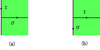
Fig. 1: T-duality transformation

We then see that this transformation exchanges Neumann condition $\partial_{\sigma}X^{\mu}=0$ and Dirichlet condition $\partial_{\tau}X^{\mu}=0$. This means that even if we start with open string theories with Neumann boundary conditions, we must have Dirichlet boundary conditions in T-dualized directions. Thus there must be some objects which fix the open string end points. Those are precisely the D-branes we mentioned before. When they have spatial $p$-dimensional extension, they are called D$p$-branes.

It has been discovered [2] that D$p$-branes have this perturbative description, and their important properties are as follows:

1. They are BPS objects, namely they preserve part of supersymmetry (typically 1/2).

2. There is no force between parallel D$p$-branes computed by the diagram in Fig. 2. This is due to the remaining supersymmetry and the exchange of (NS, NS) and (R, R) bosons cancel.

   

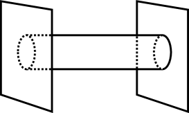
   Fig. 2: D-brane interaction

3. They are objects that carry RR charge (i.e. couple to RR forms present in type II theories). Their tension is given by

   $$\frac{1}{\alpha^{\prime}{}^{(p+1)/2}g},$$ (5.1)

   where $g$ is the string coupling constant, and their charges are quantized. This is because $p$-brane and $p^{\prime}\equiv(6-p)$-brane is dual and Dirac quantization condition must hold for the charges of these objects, just as the electrons and magnetic monopoles. (Note that $p$-brane couples to $A_{p+1}$-form, whose field strength $F_{p+2}$ is dual to $*F_{8-p}$, whose potential is $*A_{7-p}$-form which couples to $(6-p)$-brane.) As we have discussed in § 2, RR (potential) forms of odd (even) rank exist in type IIA (IIB) theory, so IIA (IIB) contains D$p$-branes with even (odd) $p$.

   The Dirac quantization condition on these charges is

   $$\mu_{p}\mu_{6-p}=2\pi n,\;\;n\in\mathbb{Z}.$$ (5.2)

   In fact, the D$p$-brane charge is given by

   $$\mu_{p}=(2\pi)^{\frac{7-2p}{2}}(\alpha^{\prime})^{\frac{3-p}{2}},$$ (5.3)

   consistent with the quantization condition (5.2). This will be important in studying black hole entropy.

4. Open strings can attach to D-branes. This means that the effective theory on the D-branes is a gauge theory. [20]

All of the above properties turned out to play very important roles in the understanding of nonperturbative properties of superstring theories.

6 T-duality of Unoriented String

Consider, in closed string, worldsheet parity transformation

$$\mathchar 28938\relax:\sigma\to 2\pi-\sigma,$$ (6.1)

and require that all the states in the theory obey

$$\mathchar 28938\relax=+1.$$ (6.2)

Physically this implies that all the states in the theory are invariant under the orientation reversal, leaving a theory of unoriented strings. If we consider T-duality in a theory with this requirement, the dual coordinate $X^{\prime}{}^{m}(z,\bar{z})=X_{L}^{m}(z)-X_{R}^{m}(\bar{z})$ transforms as

$$X^{\prime}{}^{m}(z,\bar{z})\leftrightarrow-X^{\prime}{}^{m}(z,\bar{z}),$$ (6.3)

whereas the original coordinates remain the same. The symmetry in the dual picture is then

$$\mbox{(parity transf. }\sigma\to 2\pi-\sigma)\times(\mbox{reflection in $m$ direction }X^{\prime}{}^{m}\to-X^{\prime}{}^{m}).$$ (6.4)

This requirement defines unoriented string. The target space is not a circle but a half line, which is $S^{1}/{\mathbb{Z}}_{2}$, and is called orientifold.

As a simple example of orientifold, consider a circular coordinate $-\pi R\leq x\leq\pi R$. The above ${\mathbb{Z}}_{2}$ identification makes the space

$$0\leq x\leq\pi R.$$ (6.5)

and produces fixed planes at $x=0,\pi R$, called orientifold fixed planes. Note that in this construction these are rigid fixed planes and not dynamical ones unlike D-branes.

Let us look at the theory in various aspects. Close to the orientifold, we have unoriented open strings as well as closed strings. In this way type I theory may be regarded as type IIB theory on orientifold.

Far from these fixed planes, the theory is just like the original oriented IIB string, and the unorientedness is taken care by the presence of the fixed planes which fix the motion of the strings at mirror points.

We are now ready to discuss the M-theory conjecture.

7 Strong coupling Limit of Type II Superstring

In type IIA theory, we have learned that there exist D$p$-branes for even $p$. In particular, consider D0-branes. Their properties of particular importance here include:

1. The tension or energy of D0-branes is $\frac{1}{\sqrt{\alpha^{\prime}}g}$.

2. They are BPS, so that the energy of $n$ bound states is $\frac{n}{\sqrt{\alpha^{\prime}}g},(n=1,2,\cdots)$ without binding energy.

3. Their BPS property (or supersymmetry representation theory) means that this energy is not changed by quantum corrections.

In perturbation theory, D0-branes can be neglected because they are heavy with mass inversely proportional to the coupling constant. In the strong coupling, however, they are light and the low-energy effective theory is significantly modified. Not only that, we have a huge tower of light massive states as given in item 2 above.

How can we understand such an infinite tower of light massive states?

The proposed answer is that they are just the Kaluza-Klein(KK)-modes from 11 dimensions! This is the first signal of the M-theory. There are also various other evidences for this proposal in addition to the fact that other BPS D-branes can be understood similarly.

To get more concrete relation between the 11-dimensional M-theory and superstrings, consider massless fields in type IIA theory:

$$\mbox{(NS, NS): dilaton }\phi,\mbox{ metric }g_{\mu\nu},\mbox{ antisymmetric }B_{\mu\nu},$$

$$\mbox{(R, R): forms }A_{1},A_{3}.$$ (7.1)

The (bosonic part of) the low-energy effective action (IIA supergravity) is

$$S_{\rm NS-NS} = \frac{1}{2\kappa_{10}^{2}}\int d^{10}x\sqrt{-g}e^{-2\phi}{\hbox{$\left(\vbox to0.0pt{}\right.\n@space$}}R+4(\nabla\phi)^{2}-\frac{1}{2}H^{2}{\hbox{$\left)\vbox to0.0pt{}\right.\n@space$}},$$

$$S_{R-R} = -\frac{1}{4\kappa_{10}^{2}}\int d^{10}x\sqrt{-g}{\hbox{$\left(\vbox to0.0pt{}\right.\n@space$}}F_{2}^{2}+F_{4}^{\prime}{}^{2}{\hbox{$\left)\vbox to0.0pt{}\right.\n@space$}}-\frac{1}{4\kappa_{10}^{2}}\int F_{4}\wedge F_{4}\wedge B,$$ (7.2)

where $2\kappa_{10}^{2}=16\pi G_{10}$ is the 10-dimensional Newton constant and

$$H=dB,\;\;F_{2}=dA_{1},\;\;F_{4}=dA_{3},\;\;F_{4}^{\prime}=dA_{3}+A_{1}\wedge H,$$ (7.3)

and the suffices indicate the ranks of the forms. The algebra of the two supercharges of opposite chirality $Q,Q^{\prime}$ roughly takes the form

$$\{Q,Q\}\sim\{Q^{\prime},Q^{\prime}\}\sim P,$$

$$\{Q,Q^{\prime}\}\sim W\ \ (\cdots\mbox{ central charge}).$$ (7.4)

The D-branes belong to the representation of this algebra with maximum central charges.

We can understand the origin of the central charges in (7.4) as follows: When the 11-dimensional theory is compactified on ${\mathbb{R}}^{10}\times S^{1}$, the fields in the original theory produce the gauge fields and central charges as

$$g_{\mu,11}\Rightarrow A_{1},\quad p_{11}\Rightarrow W.$$ (7.5)

Namely the central charge is nothing but the 11-th momentum and its gauge field is the RR-form originating from the 11-dimensional metric. This means that the RR charged objects are actually KK modes. Also their mass is given by $\frac{n}{R_{11}},n\in\mathbb{Z}$, which is of the same form as the mass of D0-branes. The 10-dimensional $N=2$ supersymmetry also matches with 11-dimensional supersymmetry.

Comparison of the low-energy actions (massless) tells us that we should write the 11-dimensional metric in terms of the type IIA fields as

$$ds_{11}^{2} = e^{-\frac{2}{3}\phi}g_{\mu\nu}dx^{\mu}dx^{\nu}+e^{\frac{4}{3}\phi}(dy+A_{\mu}dx^{\mu})^{2}.$$ (7.6)

This yields in fact the effective action (7.2) from the 11-dimensional action

$$S_{11}=\frac{1}{2\kappa_{11}^{2}}\int d^{11}x\sqrt{-G}\left(R-\frac{1}{2}|F_{4}|^{2}\right)-\frac{1}{12\kappa_{11}^{2}}\int A_{3}\wedge F_{4}\wedge F_{4},$$ (7.7)

where $\kappa_{11}^{2}(=2\pi R_{11}\kappa_{10}^{2})$ is the 11-dimensional Newton constant. The metric (7.6) shows that the 11-dimensional radius is given by

$$R_{11}=e^{\frac{2}{3}\phi}=g^{\frac{2}{3}}.$$ (7.8)

These results resolve several questions:

1. Perturbation in the string coupling $g$ is equivalent to the expansion around $R_{11}=0$. This is the reason why string perturbation cannot see 11-th dimension!!

2. Masses of KK modes are given by

   $$\frac{e^{-\frac{1}{3}\phi}}{R_{11}}\sim\frac{1}{g},$$ (7.9)

   which in fact matches with those of D0-branes. They are also BPS states with RR-charge, consistent with D0-branes.

In the strong coupling limit $g\to\infty,R_{11}\to\infty$ and the theory is an 11-dimensional supersymmetric theory with gravity. The low-energy effective theory (containing only massless degrees) must be the 11-dimensional supergravity which is the unique theory with this property.

We have thus learned that the strong coupling limit of type IIA theory is the M-theory. What about the strong coupling limit of type IIB theory?

Consider the metrics for IIA and IIB compactified on $S^{1}$ of radii $R_{A}$ and $R_{B}$, respectively. The T-duality relation of these theories implies that the metrics are written as

$${\rm IIB}/R_{\rm B} : ds^{2}=\cdots+g_{99}(dx^{9})^{2},$$

$${\rm IIA}/R_{\rm A} : ds^{2}=\cdots+\frac{1}{g_{99}}(dx^{9})^{2},\quad g_{99}=e^{2(\phi_{B}-\phi_{A})},$$ (7.10)

$$R_{A}=e^{\phi_{A}-\phi_{B}},\quad R_{B}=e^{-\phi_{A}+\phi_{B}},$$

where $\phi_{A,B}$ are the dilatons in each theory. When these theories are regarded as M-theory compactified on $T^{2}$ of radii $R_{10},R_{11}$, the relation (7.6)

$$ds_{11}^{2}=e^{-\frac{2}{3}\phi_{A}}ds_{10}^{2}+e^{\frac{4}{3}\phi_{A}}(dy+A_{\mu}dx^{\mu})^{2},$$ (7.11)

yields $R_{10}=e^{-\frac{1}{3}\phi_{A}}R_{A}$. A simple manipulation of metrics and radii using relations given in (7.10) gives the type IIB coupling as

$$g^{(B)}(\equiv e^{\phi_{B}})=\frac{R_{11}}{R_{10}}.$$ (7.12)

Since $R_{10}$ and $R_{11}$ are completely on the same footing, we thus find that the IIB theory is invariant under

$$g^{(B)}\to\frac{1}{g^{(B)}}.$$ (7.13)

Consequently the strong coupling limit of IIB is itself! More generally, it is known the effective type IIB supergravity is invariant under $SL(2,{\mathbb{Z}}_{2})$ transformation

$$\tau\to\frac{a\tau+b}{c\tau+d};\;\;\tau\equiv l+ie^{-\phi_{B}},\quad a,b,c,d\mbox{: integers},\;\;(ad-bc=1),$$ (7.14)

where $l$ is an RR scalar field. Note that (7.14) reproduces (7.13) for $l=0$ and $a=d=0,b=-c=1$. It is believed that the complete type IIB superstring (not only the massless sector) has this invariance. There is also another evidence supporting this conjecture.

Thus we have learned

IIB	$\Leftrightarrow$	IIB	$\Leftrightarrow$	IIA	$\to$	11-dim. M-theory
	strong		T-duality		strong
	coupling		$R\leftrightarrow\frac{\alpha^{\prime}}{R}$		coupling
					$R_{11}\to\infty$

The overall picture is like in Fig. 3.

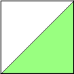
Fig. 3: IIB or not IIB

8 $SO(32)$ Type I and Heterotic Strings

Once the evidence for the existence of the unifying M-theory was discovered, it was quickly accepted and duality for other superstring theories was easily found. In the following few sections, we will briefly summarize the evidence of the dualities of all superstring theories.

The first is the duality between $SO(32)$ type I and heterotic strings. [21] We note that $SO(32)$ type I theory possesses $D=10,N=1$ supersymmetry. This theory contains open and closed strings in the weak coupling picture. The question we address here is what happens in the strong coupling limit of this theory.

We first note that the maximum spin in the massive representations of $D=10,N=1$ supersymmetry algebra is 2. It is impossible that these massive spin 2 particles become massless in the strong coupling limit and the theory is promoted to 11-dimensional theory, because 11-dimensional theory has bigger ($N=2$) supersymmetry and no gauge particles.

The only possibility would be then to reduce to again 10-dimensional theory, which cannot be itself because there is no $SL(2,{\mathbb{Z}}_{2})$-like symmetry in type I theory (contrary to IIB). It turns out that the theory we reach is the heterotic $SO(32)$ theory in the strong coupling limit.

$SO(32)$ type I theory	$\Leftrightarrow$	heterotic $SO(32)$ theory
	S-dual

Let us check this relation by comparing the low-energy effective theories. The type I effective theory is given by

$$S_{I} = \frac{1}{2\kappa_{10}^{2}}\int d^{10}x\sqrt{-G}\left\{e^{-2\phi}(R+4(\partial_{\mu}\phi)^{2})-\frac{1}{2}|\tilde{F}_{3}|^{2}\right\}$$ (8.1)

$$-\frac{1}{2g_{10}^{2}}\int d^{10}x\sqrt{-G}e^{-\phi}{\rm Tr}|F_{2}|^{2},$$

where $\tilde{F}_{3}=dC_{2}-\frac{\kappa_{10}^{2}}{g_{10}^{2}}\omega_{3},\omega_{3}={\rm Tr}(A_{1}\wedge dA_{1}-\frac{2}{3}iA_{1}^{3})$, and $g_{10}$ is the SYM coupling constant. On the other hand, the $SO(32)$ heterotic effective theory is given by

$$S_{H} = \frac{1}{2\kappa_{10}^{2}}\int d^{10}x\sqrt{-G}e^{-2\phi}{\hbox{$\left\{\vbox to0.0pt{}\right.\n@space$}}R+4(\partial_{\mu}\phi)^{2}-\frac{1}{2}|\tilde{H}_{3}|^{2}-\frac{\kappa_{10}^{2}}{g_{10}^{2}}{\rm Tr}|F_{2}|^{2}{\hbox{$\left\}\vbox to0.0pt{}\right.\n@space$}},$$ (8.2)

where $\tilde{H}_{3}=dB_{2}-\frac{\kappa_{10}^{2}}{g_{10}^{2}}\omega_{3}.$ It is easy to see that these two effective theories are related by

$$\begin{array}[]{ll}G_{I\mu\nu}=e^{-\phi_{H}}G_{H\mu\nu},&\phi_{I}=-\phi_{H},\\ \tilde{F}_{I3}=\tilde{H}_{H3},&A_{I1}=A_{H1},\end{array}$$ (8.5)

in agreement with the above assertion.

9 Two Heterotic Strings

Using the similar argument, it is not difficult to show that there is a relation between two heterotic string theories with $SO(32)$ and $E_{8}\times E_{8}$ symmetries under T-duality. [22] In order to show this, we have to first break the gauge symmetries to the common $SO(16)\times SO(16)$ symmetry by introducing Wilson lines in the moduli space of the theories, and then use the properties of the even self-dual lattice in the moduli space to argue the equivalence of the resulting theories. In this way it has been shown that these theories are transformed into each other under T-duality transformation. Schematically this is written as

$SO(32)$ heterotic	$\Leftrightarrow$	$E_{8}\times E_{8}$ heterotic
$\downarrow$	$S^{1}$ with	$\downarrow$
	Wilson line
$SO(16)\times SO(16)$ heterotic	$\Leftrightarrow$	$SO(16)\times SO(16)$ heterotic
	T-dual

and hence

$SO(32)$ heterotic	$\Leftrightarrow$	$E_{8}\times E_{8}$ heterotic
	T-dual

10 String Web — Overall picture

What we have learned so far can be summarized in the following diagram:

11D	M-theory
	$|S^{1}$
10D	IIA	$\Leftrightarrow$	IIB
		T	$|S^{1}/{\mathbb{Z}}_{2}$
9D			type I	$\Leftrightarrow$	$SO(32)$ heterotic	$\Leftrightarrow$	$E_{8}\times E_{8}$ heterotic
				S		T

This already indicates that all superstrings are dual. Using this relation and the connection between IIB and I superstrings discussed in § 6, we start with M-theory compactified on $S^{1}\times S^{1}/{\mathbb{Z}}_{2}$ and end with $E_{8}\times E_{8}$ heterotic theory on $S^{1}$ by the following route:

M/$S^{1}\times S^{1}/{\mathbb{Z}}_{2}$	$\to$	IIA/$S^{1}/{\mathbb{Z}}_{2}$	$\to$	IIB/$S^{1}/{\mathbb{Z}}_{2}$
	S		T	$\downarrow$
$E_{8}\times E_{8}$ heterotic/$S^{1}$	$\leftarrow$	$SO(32)$ heterotic/$S^{1}$	$\leftarrow$	I/$S^{1}$
	T		S

Comparing the both ends, we arrive at the conjecture by Hořava and Witten [23]

$$\mbox{M/$(S^{1}/{\mathbb{Z}}_{2})$ = $E_{8}\times E_{8}$ heterotic}.$$ (10.1)

As we have discussed in § 6, $S^{1}/{\mathbb{Z}}_{2}$ is an orientifold, a line with fixed planes on both ends.

There are several supporting evidences for this conjecture: First, the low-energy limit of the M-theory is the 11-dimensional supergravity. The above compactification (10.1) is consistent with the 11-dimensional supergravity because it is invariant under ${\mathbb{Z}}_{2}$ if $A^{(3)}\to-A^{(3)}$ so that we can consider this compactification.

Second, it is consistent with supersymmetry. M/${\mathbb{R}}^{10}\times S^{1}$ is invariant under supersymmetry with arbitrary $\epsilon$ (32 components), namely this gives $N=2$ in 10 dimensions. ${\mathbb{Z}}_{2}$ action kills half of the supersymmetry, because unbroken supersymmetry is determined by the condition $\mathchar 28928\relax^{11}\epsilon=\epsilon$. This also means that $\epsilon$ is chiral in 10 dimensions, consistent with the supersymmetry of the heterotic string! It follows that M/${\mathbb{R}}^{10}\times S^{1}/{\mathbb{Z}}_{2}$ reduces to 10-dimensional Poincaré-invariant theory with one chiral supersymmetry. There are three candidates satisfying this criterion: $E_{8}\times E_{8}$ heterotic, $SO(32)$ heterotic, and $SO(32)$ type I theories. Which is the one we are looking for?

The answer is given by the following considerations, all of which point to $E_{8}\times E_{8}$ heterotic theory.

(i) gravitational anomaly
The effective action must be invariant under diffeomorphism. On smooth 11-dimensional manifold, the theory is anomaly free. However, when it is compactified on orientifold, 11-dimensional Rarita-Schwinger field produces not only infinitely many massive fields (which are anomaly free) but also massless chiral 10-dimensional gravitini which may produce anomaly.

The absence of anomalies in 11 dimensions implies that the anomalies do not exist at smooth point in ${\mathbb{R}}^{10}\times S^{1}/{\mathbb{Z}}_{2}$. It then follows that the possible anomalies are sum of delta functions on the fixed hyperplanes at $x^{11}=0,\pi R$. By symmetry, the form of anomalies at $x^{11}=0,\pi R$ must be the same. Since the anomaly is not zero, there must be additional massless modes that propagate only on the fixed planes and cancel those from gravitini. They must be 10-dimensional fields, and the only candidates are the 10-dimensional vector multiplets. In 10 dimensions, standard anomaly can be canceled only by 496 vector multiplets, which are divided equally between the two fixed hyperplanes. Consequently 248 vector multiplets must exist on each hyperplane, implying that they must be $E_{8}\times E_{8}$ gauge particles. $SO(32)$ is impossible because that would require all the vector multiplets on one hyperplane.

(ii) Strong coupling behavior
If M-theory on ${\mathbb{R}}^{10}\times S^{1}/{\mathbb{Z}}_{2}$ of radius $R$ is equivalent to $E_{8}\times E_{8}$ heterotic string with coupling constant $g$, we have $R=g^{2/3}$. This means that when $R$ is small, string picture is a good description. When $R$ is large, on the other hand, supergravity description is good. It follows that the relation can be well studied in the supergravity approximation.

Now we already know (in § 8) that the strong coupling limit of type I superstring in 10 dimensions is again a 10-dimensional weakly coupled $SO(32)$ heterotic string, and hence these two are not related to 11-dimensional supergravity in the strong coupling or large $R$ limit. The only possibility left is then that the orientifold theory in the large $R$ limit is related to $E_{8}\times E_{8}$ heterotic string.

Thus all evidences support the conjecture that the M-theory compactified on $S^{1}/{\mathbb{Z}}_{2}$ is the $E_{8}\times E_{8}$ heterotic theory.

In this way all consistent superstrings are related with each other by S-duality or T-duality. This completes the whole picture of the string web.

11 D-branes in Type II Supergravity and Black Holes

We now go on to describe the same D-branes as the classical soliton solutions in the low-energy effective theory (supergravity). This allows us to understand the geometry of the space-time produced by D-branes, and gives black hole interpretation of these solutions.

The massless degrees of freedom in the theories are gravity + dilaton + antisymmtric tensors (plus fermions which are irrelevant to our following discussions). The effective actions are uniquely determined by 10- or 11-dimensional supersymmetry. They allow various brane solutions as solitons. Most important are the D-branes. The previous description of D-branes is in terms of perturbative string picture. Here the D-branes are identified as the classical solitonic solutions in supergravity.

The bases to identify these classical solutions as D-branes are:

1. They are spatially $p$-dimensional extended BPS objects with 1/2 supersymmetry.

2. They carry RR charges.

The important assumption is that the physical contents of the theory do not change if coupling constant is changed because of the remaining supersymmetry (BPS representation). This means that there are two ways of description of the same objects – D-branes – by open and closed string degrees of freedom.

Example: Let us consider 2-brane solution in $D=11$

$$ds^{2} = H^{1/3}[H^{-1}(-dt^{2}+dy_{1}^{2}+dy_{2}^{2})+dr^{2}+r^{2}d\mathchar 28938\relax_{7}^{2}],$$ (11.2)

$$A_{\mu\nu\lambda}=\epsilon_{\mu\nu\lambda}H^{-1},\;H\equiv 1+\frac{k}{r^{6}}.$$

We regard the 8-dimensional space described by $r$ and angular coordinates as our space-time. The metric is invariant in $y_{1},y_{2}$ directions, and is asymptotically flat in other directions. This means that there is some object extended in $y_{1},y_{2}$, which deserves the name of 2-brane or membrane.

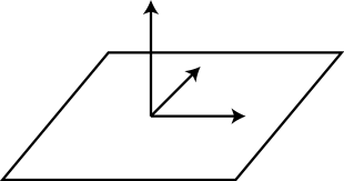
Fig. 4: Membrane

Now take the Schwarzschild-type coordinates $r=(\tilde{r}^{6}-k)^{1/6}$, and the metric is written as

$$ds^{2}=(1-k/\tilde{r}^{6})^{2/3}(-dt^{2}+dy_{1}^{2}+dy_{2}^{2})+(1-k/\tilde{r}^{6})^{-2}d\tilde{r}^{2}+\tilde{r}^{2}d\mathchar 28938\relax_{7}^{2}.$$ (11.3)

If $y_{1}$ and $y_{2}$ are compactified, we see that this describes a black hole geometry with a horizon at $\tilde{r}=k^{1/6}$, but a time-like and space-like vectors are not interchanged upon crossing it. The causal structure of this space-time is depicted in Fig. 5.

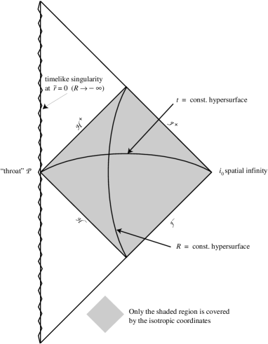
Fig. 5: Carter-Penrose diagram for M2-brane. [5] Here $R=(1-k/\tilde{r}^{6})^{1/3}$.

We find that the global structure is similar to the Reissner-Nordstrom solution.

Similar extended brane solutions in superstring theories are summarized in the following table:

type IIA	type IIB
fundamental string	fundamental string
D$p$-branes ($p$: even)	D$p$-branes ($p$: odd)
NS5-brane	NS5-brane
KK-wave	KK-wave

More general solutions can be constructed by combining these solutions. [24, 25, 26, 27] The construction rules are called intersection rules. Combining these according to the intersection rules, it is possible to make solutions that can be interpreted as $D=4,5$ black holes.

Example: Type IIB D5-D1-KK-wave intersecting solution is given by

$$ds^{2}=H_{1}^{-\frac{3}{4}}H_{5}^{-\frac{1}{4}}[-(1-r_{0}^{2}/r^{2})dt^{2}+dx_{9}^{2}+(r_{0}^{2}/r^{2})(\cosh\sigma dt+\sinh\sigma dx_{9})^{2}]$$

$$+H_{1}^{\frac{1}{4}}H_{5}^{-\frac{1}{4}}[dx_{5}^{2}+dx_{6}^{2}+dx_{7}^{2}+dx_{8}^{2}]+H_{1}^{\frac{1}{4}}H_{5}^{\frac{3}{4}}[(1-r_{0}^{2}/r^{2})^{-1}dr^{2}+dr^{2}\mathchar 28938\relax_{3}^{2}],$$ (11.4)

where $r^{2}=x_{1}^{2}+\cdots+x_{4}^{2},H_{i}=1+\frac{r_{0}^{2}}{r^{2}}\sinh\alpha_{i}$, $x_{5},\cdots,x_{9}$ are compactified on a torus $T^{5}$ of radii $R_{5},\cdots,R_{9}$, giving $D=5$ black hole.

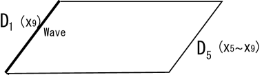
Fig. 6: D1-D5-Wave intersecting solution

Remember that the D-brane charges are quantized. This leads to the result that the Bekenstein-Hawking entropy

$$S=\frac{\rm area}{4}=2\pi\sqrt{Q_{1}Q_{5}N},$$ (11.5)

is quantized, where $Q_{1},Q_{5}$ and $N$ are the (integer) numbers of D1-, D5-branes and momentum!! This is already quite a nontrivial result which is obtained from the brane realization of black hole solutions.

Now we are going to use another description of this black hole or D-brane solutions in terms of perturbative string picture to give explanation of the entropy (11.5) by statistical mechanics. The existence of the D-branes is probed by open string. This means that if there is only one D-brane, $U(1)$ gauge theory is realized on the D-brane. If there are two separate D-branes, then $U(1)\times U(1)$ plus open strings between the 2 D-branes exist. When these 2 D-branes are on top of each other, gauge symmetry is enhanced to $U(2)$. Thus $Q_{5}$ D-branes at the same position give rise to $U(Q_{5})$ gauge theory on the world-volume!

Using this description, we can count the degrees of freedom living on the above solution. The system can be regarded as gas of $N_{B}=N_{F}=4Q_{1}Q_{5}$ massless particles with energy $E=N/R_{9}$ in a space of length $L=2\pi R_{9}$, giving the entropy precisely agreeing with (11.5). We thus get precise agreement of the black hole entropy, calculated from Bekenstein-Hawking formula and from this string picture. [6, 7]

This gives the statistical origin of the black hole entropy. The upshot is that the information is stored on the brane or horizon, and the counting of the degrees of freedom on them gives the statistical mechanical entropy which coincide with the Bekenstein-Hawking entropy (11.5). This is a kind of holographic principle, meaning that information is stored on the boundary.

This is also one of the manifestations of the equivalent descriptions (duality) of the theory in terms of open and closed string degrees of freedom. We are now going to describe another manifestation of this duality under the name of AdS/CFT correspondence.

12 AdS/CFT Correspondence

Let us consider S-channel and T-channel duality depicted in the following diagrams in Fig. 7:

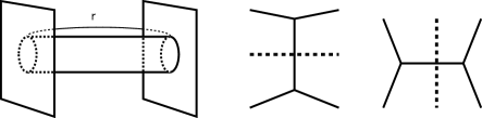
Fig. 7: S- and T-channel duality

The claim is that the latter two diagrams give the same amplitudes in string theories. When applied to the first diagram, this shows the remarkable property of the string theory that the open string one loop diagram is equivalent to that of closed string exchange. This equivalence is valid after sum over all modes. When the distance $r$ of closed string propagation is small, this process can be better described by open strings, or in terms of SYM theories. However, when the length $r$ of open string is large, it is better described by closed strings, or in terms of supergravity.

This correspondence or duality of the two descriptions may be best explained by the following example of D3-branes:

$$ds^{2}=H^{-\frac{1}{2}}(-dt^{2}+dy_{1}^{2}+dy_{2}^{2}+dy_{3}^{2})+H^{\frac{1}{2}}(dr^{2}+r^{2}d\mathchar 28938\relax_{5}^{2}),$$ (12.1)

Near branes ($r\sim 0$), description by open strings is good and the theory is well described by $D=4,N=4$ SYM theory. This theory possess superconformal symmetry including $SO(2,4)$. On the other hand, the same theory may be expected to be well described by the near-horizon geometry in supergravity solution (12.1) for certain region of coupling constant. Near the horizon, (12.1) is approximated as

$$ds^{2}\sim\alpha^{\prime}{\hbox{$\left[\vbox to0.0pt{}\right.\n@space$}}\frac{u^{2}}{\sqrt{4\pi gN}}dx_{4}^{2}+\sqrt{4\pi gN}{\hbox{$\left(\vbox to0.0pt{}\right.\n@space$}}\frac{du^{2}}{u^{2}}+d\mathchar 28938\relax_{5}^{2}{\hbox{$\left)\vbox to0.0pt{}\right.\n@space$}}{\hbox{$\left]\vbox to0.0pt{}\right.\n@space$}},$$ (12.2)

where $u\simeq r/\alpha^{\prime}$ is fixed. (Here $u$ gives the energy scale we are looking at the theory, and fixing $u$ means that we are keeping the stretched open string mass finite.) This is a space of direct product of AdS${}_{5}\times S^{5}$ with the same superconformal symmetry including $SO(2,4)\times SO(6)$.

It has been proposed that the above $D=4,N=4$ superconformal theory is well described by this AdS solution (12.2). [8] The evidences that the above two descriptions are valid include:

1. Agreement of symmetries, as shown above.

2. Agreement of spectrum.

3. Agreement of operator algebra.

This is what is called AdS/CFT correspondence or duality, meaning that there are different descriptions of the same object valid for different regions of coupling constant etc. This is closely related to ’t Hooft’s old idea that the large $N$ gauge theory (open string) is related to string (closed string) in the confining phase.

Note that the curvature for the metric (12.2) is proportional to $\frac{1}{\sqrt{4\pi gN}}$, so supergravity description is good in the large $gN$ but small $g$ limit, and hence in the large $N$ limit. Otherwise we have to consider full string theory.

The rules for practical calculations are formulated in refs. ?, ? and they are based on the following observations: In AdS background, the bulk field $\phi$ is completely determined by its field equation and given boundary values $\phi(\mathchar 28938\relax)$. Hence the action gives the generating functional of the correlation functions for the local operators on the boundary which couple to the boundary value of the fields.

$$e^{iS_{eff}(\phi_{i})}={\langle}Te^{i\int_{B}\phi_{b,i}{\cal O}^{i}}\rangle$$ (12.3)

In the next section, we give greybody factors for BTZ black holes by using this idea. [28, 29, 30]

Before going into details, let us summarize properties of AdS_p+2 space, which is a space with $R_{\mu\nu}=\frac{\mathchar 28931\relax}{D-2}g_{\mu\nu}$ with $D>2,\mathchar 28931\relax<0$. Namely AdS_p+2 is a space with negative cosmological constant. A convenient description of the space is to use the embedding in flat $(p+3)$-dimensional space-time:

$$-y_{-1}^{2}-y_{0}^{2}+y_{1}^{2}+\cdots+y_{p+1}^{2}=-R^{2},$$ (12.4)

with $SO(2,p+1)$ isometry.

$$ds^{2}=-dy_{-1}^{2}-dy_{0}^{2}+dy_{1}^{2}+\cdots+dy_{p+1}^{2},$$ (12.5)

Put

$$r=y_{-1}+y_{p+1},\;\;\;v=y_{-1}-y_{p+1},\;\;\;x_{i}=(R/r)y_{1},$$ (12.6)

and we get

$$ds^{2}=\frac{r^{2}}{R^{2}}dx^{2}+\frac{R^{2}}{r^{2}}dr^{2}=R^{2}(U^{2}dx^{2}+\frac{dr^{2}}{U^{2}}),\;\;\;U=\frac{r}{R^{2}}.$$ (12.7)

For $p=3$, this has the same symmetry as $N=4,D=4$ SCFT with $SO(2,4)$, leading to the conjecture that the strong coupling SYM is equivalent to the weak coupling supergravity.

Finally let us summarize the known examples of AdS_p+2/CFT_p+1 correspondence in the following table:

M-theory	M2 ($p=2$)	AdS4/CFT3
	M5 ($p=5$)	AdS7/CFT6
IIB	D3	AdS5/CFT4
	D1 + D5 on T4	AdS3/CFT2

The last one is the AdS₃/CFT₂ correspondence best checked.

Related results and future directions:

• The entropy for BTZ (and higher-dim.) black hole can be computed using the central charge of the Virasoro algebra realized on the boundary geometry without recourse to supersymmetry. [31, 32]

• The properties of gravity, in particular the evolution of Hawking radiation and the information loss, can be studied by well-behaved, unitary conformal field theory. If true, this suggests that the problem of information loss is actually not present.

• It may be even possible to formulate “string theory” in terms of field theory. A partial realization of this idea is what is called Matrix theory. [12]

We now discuss two applications of AdS/CFT correspondence in the following two sections.

13 Greybody Factors for BTZ Black Hole

Consider the 3-dimensional BTZ black hole. When embedded in string theory, this can be related to other 5D and 4D black holes, whose metric is

$$ds_{10}^{2} = -\frac{(\rho^{2}-\rho_{-}^{2})(\rho^{2}-\rho_{+}^{2})}{l^{2}\rho^{2}}dt^{2}+\rho^{2}\left(d\varphi-\frac{\rho_{+}\rho_{-}}{l\rho^{2}}dt\right)^{2}$$ (13.1)

$$+\frac{l^{2}\rho^{2}}{(\rho^{2}-\rho_{+}^{2})(\rho^{2}-\rho_{-}^{2})}d\rho^{2}+l^{2}d\mathchar 28938\relax_{3}^{2}+dy_{2}^{2}+\cdots+dy_{4}^{2}.$$

The first part is the metric for BTZ black hole! Thus the entropies of 5D and 4D black holes may be related to those of BTZ black holes.[28, 29, 30] We now claim that not only the entropy of black hole but also absorption cross sections or greybody factors can be examined by going to AdS₃ and using the AdS/CFT correspondence.

The basic idea is the following: The greybody factors can be evaluated for BTZ black holes through the discontinuity of the two-point correlation functions (optical theorem) evaluated from AdS/CFT correspondence.

In AdS space in the Poincaré coordinate

$$ds^{2}=\frac{l^{2}}{y^{2}}(dy^{2}+dw_{+}dw_{-}),$$ (13.2)

we consider massive scalar field with mass $m$:

$$S(\phi)=\frac{1}{2}\int dydw_{+}dw_{-}\sqrt{g}\left(g^{\mu\nu}\partial_{\mu}\phi\partial_{\nu}\phi+m^{2}\phi^{2}\right),$$ (13.3)

which has a solution with the behavior

$$\phi(y,w_{+},w_{-})\to y^{2h_{-}}\phi_{0}(w_{+},w_{-}),$$ (13.4)

for $y\to 0$ (boundary), with the dimension of the boundary value $\phi_{0}(w_{+},w_{-})$ and

$$h_{\pm}=\frac{1}{2}(1\pm\sqrt{1+m^{2}}).$$ (13.5)

The main steps in our calculations are:

1. Evaluate the two-point function by AdS/CFT correspondence.

2. Obtain the greybody factors in BTZ black holes from the discontinuity of the two-point correlation function (optical theorem).

After this procedure, we find [29]

$$\sigma_{abs} = \frac{\pi}{\omega}\int dt\int_{-\infty}^{\infty}d\varphi e^{ip\cdot x}[G(t-i\epsilon,\varphi)-G(t+i\epsilon,\varphi)]$$ (13.6)

$$= \frac{2h_{+}(2h_{+}-1)(2\pi T_{+}l)^{2h_{+}-1}(2\pi T_{-}l)^{2h_{+}-1}\sinh\left(\frac{\omega}{2T_{H}}\right)}{\omega\mathchar 28928\relax^{2}(2h_{+})}$$

$$\times\left|\mathchar 28928\relax\left(h_{+}+i\frac{\omega}{4\pi T_{+}}\right)\mathchar 28928\relax\left(h_{+}+i\frac{\omega}{4\pi T_{-}}\right)\right|^{2},$$

where

$$\frac{2}{T_{H}}=\frac{1}{T_{+}}+\frac{1}{T_{-}},\quad T_{\pm}\equiv\frac{\rho_{+}\mp\rho_{-}}{2\pi}.$$ (13.7)

We can read off the decay rate for massless scalar field from this result:

$$\mathchar 28928\relax = \frac{\sigma_{abs}(h_{+}=1)}{e^{\omega/T_{H}}-1}$$ (13.8)

$$= \frac{\omega\pi^{2}l^{2}}{(e^{\omega/2T_{+}}-1)(e^{\omega/2T_{-}}-1)},$$

consistent with the semiclassical gravity calculations, giving another evidence of the duality.

The initial state of BTZ black holes was described by Poincaré vacuum, and the calculation involves a nonlinear coordinate transformation, which induces the Bogoliubov transformation on the operators. This is the origin of the thermal factor in the above.

It is possible to use the above results and methods to evaluate similar quantities in 4D and 5D black holes, and also for fermions. [33]

14 Dual Gravity Description of Noncommutative Super Yang-Mills

If one introduces constant background $B$ field on the D-branes, it produces noncommutative SYM theory on the branes, and in an appropriate limit one can define noncommutative field theory decoupled from gravity. [34] The generalization of AdS/CFT correspondence is possible. [35, 36, 37] The theory can be described either by noncommutative field theory or dual gravity which is asymptotically AdS but significantly deviates from AdS in the short distance. The gravity solution has nonextreme generalization with horizon, which corresponds to field theory at finite temperature (the extreme case corresponds to zero temperature).

Naively noncommutative space is “discretized” because of the “uncertainty relations” arising from the noncommutativity $[x^{\mu},x^{\nu}]=ic^{\mu\nu}$, so that one would expect that the degrees of freedom are less than the ordinary theories. On the other hand, the interactions in noncommutative theories involve higher derivatives (in the $\star$-product), so that one might expect opposite. Which is correct?

By comparing thermodynamic quantities (energy, entropy and temperature) computed in the gravity side for both commutative (AdS) and noncommutative (non-AdS) cases, we can show that the degrees of freedom in these theories are the same in the leading order in the large $N$ limit ($N$ is the number of colors for $SU(N)$ theories). [37, 38] Thus the dual gravity description is quite useful to examine problems in field theories.

15 Cardy-Verlinde Formula

The holographic principle states that for a given volume $V$, the state of maximal entropy is given by the largest black hole that fits inside $V$. The microscopic entropy $S$ associated with the volume $V$ is less than the Bekenstein-Hawking entropy:

$$S\leq\frac{\rm area}{4G}.$$ (15.1)

Verlinde observed that this bound is modified in the cosmological setting and in arbitrary dimensions. [39] His main observations are the followings:

1. Consider the space-time with the metric for the Einstein universe

   $$ds^{2}=-dt^{2}+R^{2}d\mathchar 28938\relax_{n}^{2},$$ (15.2)

   where $d\mathchar 28938\relax^{2}_{n}$ is the line element of a unit $n$-dimensional sphere. The entropy of the CFT in this space-time can be reproduced in terms of its total energy $E$ and Casimir energy $E_{c}$ by a generalized form of the Cardy-Verlinde formula as

   $$S=\frac{2\pi R}{n}\sqrt{E_{c}(2E-E_{c})}.$$ (15.3)

   (The original Cardy formula is for 2D CFT.)

2. For an $(n+1)$-dimensional closed universe, the FRW equations are

   $$H^{2}=\frac{16\pi G_{n}}{n(n-1)}\frac{E}{V}-\frac{1}{R^{2}},$$ (15.4)

   $$\dot{H}=-\frac{8\pi G_{n}}{n-1}\left(\frac{E}{V}+p\right)+\frac{1}{R^{2}},$$ (15.5)

   where $H=\dot{R}/R$ is the Hubble parameter, dot stands for differentiation with respect to the proper time, $E$ is the total energy of matter filling the universe, $p$ the pressure, $V=R^{n}\mbox{Vol}(S^{n})$ the volume of the universe, and finally $G_{n}$ is the $(n+1)$-dimensional gravitational constant. The FRW equation can be related to three cosmological entropy bounds:

   1. Bekenstein-Verlinde bound:

      $$S_{\rm BV}=\frac{2\pi}{n}ER.$$ (15.6)

      (For a system with limited self-energy, the total entropy is less than the product of energy and linear size of the system.)

   2. Bekenstein-Hawking bound:

      $$S_{\rm BH}=(n-1)\frac{V}{4G_{n}R}.$$ (15.7)

      (Black hole entropy is bounded by the area.)

   3. Hubble bound:

      $$S_{\rm H}=(n-1)\frac{HV}{4G_{n}}.$$ (15.8)

      (Maximal entropy is produced by black holes of the size of Hubble horizon.)

At the critical point defined by $HR=1$, these three entropy bounds coincide with each other.

Define $E_{\rm BH}$ such that

$$S_{\rm BH}=(n-1)V/4G_{n}R\equiv 2\pi E_{\rm BH}R/n.$$ (15.9)

The FRW equation then takes the form

$$S_{\rm H}=\frac{2\pi R}{n}\sqrt{E_{\rm BH}(2E-E_{\rm BH})},$$ (15.10)

which is of the same form as the Cardy-Verlinde formula (15.3)! Its maximum reproduces Hubble bound

$$S_{H}\leq\frac{2\pi R}{n}E.$$ (15.11)

Thus the FRW equation somehow knows the entropy of CFTs filling the universe. This connection between the Cardy-Verlinde formula and the FRW equation can be interpreted as a consequence of the holographic principle.

Our purpose is to show that it is possible to extend this holographic connection to the AdS Reissner-Nordström (RN) black hole background in arbitrary dimensions. [40]

15.1 Bekenstein Bound in Arbitrary Dimensions

The Bekenstein bound

$$S\leq S_{\rm B}=2\pi RE,$$ (15.12)

is valid for a system with the limited self-gravity (i.e. if the gravitational self-energy is negligibly small compared to its total energy).

It is known that the form of the Bekenstein bound (15.12) is independent of the spatial dimensions, and that the $D(\geq 4)$-dimensional Schwarzschild black hole satisfies the bound. The bound is saturated even for a four-dimensional Schwarzschild black hole which is a strongly self-gravitating object, but is no longer saturated for $D>4$.

For charged objects with charge $Q$ in 4 dimensions, the Bekenstein bound (15.12) is modified to

$$S\leq S_{\rm B}=\pi(2ER-Q^{2}).$$ (15.13)

The question then arises: Does this form remain unchanged in arbitrary dimensions ($D\geq 4$)?

Consider an $(n+2)$-dimensional Einstein-Maxwell theory with a cosmological constant $\mathchar 28931\relax_{\pm}=\pm n(n+1)/2l^{2}$:

$$I=\frac{1}{16\pi\bf G_{n}}\int d^{n+2}x\sqrt{-g}\left({\cal R}-F_{\mu\nu}F^{\mu\nu}-2\mathchar 28931\relax_{\pm}\right),$$ (15.14)

where ${\cal R}$is the curvature scalar, $F$ the Maxwell field, and $\bf G_{n}$ the gravitational constant in ($n+2)$ dimensions. Let us discuss a spherically symmetric solution in this theory:

$$ds^{2}=-f_{\pm}(r)dt^{2}+f_{\pm}(r)^{-1}dr^{2}+r^{2}d\mathchar 28938\relax_{n}^{2},$$ (15.15)

where

$$F_{rt}=\frac{n\omega_{n}}{4}\frac{Q}{r^{n}},\ \ \ \ \omega_{n}=\frac{16\pi\bf G_{n}}{n\mbox{Vol}(S^{n})},$$ (15.16)

$$f_{\pm}(r)=1-\frac{\omega_{n}M}{r^{n-1}}+\frac{n\omega^{2}_{n}Q^{2}}{8(n-1)r^{2(n-1)}}-\frac{2\mathchar 28931\relax_{\pm}r^{2}}{n(n+1)}.$$ (15.17)

where $\mbox{Vol}(S^{n})$ is the volume of a unit $n$-sphere.

This solution is asymptotically de Sitter (dS) or anti-de Sitter (AdS) depending on the cosmological constant $\mathchar 28931\relax_{+}$ or $\mathchar 28931\relax_{-}$. We consider the de Sitter case in this subsection.

If we put $M=Q=0$, the solution describes dS space with a cosmological horizon at $r=r_{0}\equiv\sqrt{l^{2}}$. The cosmological horizon behaves like the black hole horizon, and it has the thermodynamic entropy

$$S_{0}=\frac{r_{0}^{n}}{4\bf G_{n}}\mbox{Vol}(S^{n}).$$ (15.18)

In a general case with nonvanishing $M$ and $Q$, the solution describes the geometry of a certain object with mass $M$ and electric charge $Q$ in dS space. The cosmological horizon will shrink due to the nonzero $M$ and $Q$. This leads to the bound

$$S_{m}\leq S_{0}-S_{c},$$ (15.19)

where $S_{c}$ is the cosmological horizon entropy when matter is present.

We now estimate $S_{c}$. The cosmological horizon $r_{c}$ is given by the maximal root of the equation:

$$1-\frac{\omega_{n}M}{r_{c}^{n-1}}+\frac{n\omega_{n}^{2}Q^{2}}{8(n-1)r_{c}^{2(n-1)}}-\frac{r_{c}^{2}}{r_{0}^{2}}=0.$$ (15.20)

This leads to

$$\frac{r_{0}^{n}}{r_{c}^{n}}=\left(1-\frac{\omega_{n}M}{r_{c}^{n-1}}+\frac{n\omega_{n}^{2}Q^{2}}{8(n-1)r_{c}^{2(n-1)}}\right)^{-n/2}.$$ (15.21)

In the large cosmological horizon limit: $M/r_{c}^{n-1}\ll 1,Q^{2}/r_{c}^{2(n-1)}\ll 1$, we get

$$S_{m} \leq \frac{\mbox{Vol}(S^{n})}{4\bf G_{n}}(r_{0}^{n}-r_{c}^{n})$$ (15.22)

$$\leq 2\pi r_{c}\left(M-\frac{2\pi{\bf G_{n}}Q^{2}}{(n-1)\mbox{Vol}(S^{n})r_{c}^{n-1}}\right).$$

The entropy reaches its maximum when the matter extends to the cosmological horizon. If we replace $r_{c}$ by $R$ and $M$ by the proper energy $E$, we obtain the entropy bound of the charged object in arbitrary dimensions ($D=n+2\geq 4$):

$$S\leq S_{\rm B}=2\pi R\left(E-\frac{2\pi{\bf G_{n}}Q^{2}}{(n-1)\mbox{Vol}(S^{n})R^{n-1}}\right).$$ (15.23)

Let us make various checks of this formula:

• This bound is satisfied by RN black holes in arbitrary dimensions.

• When $Q^{2}=0$, this bound reproduces precisely the Bekenstein bound for the neutral object in arbitrary dimensions.

• For $n=2$, the entropy bound reduces to the four-dimensional one.

These confirm the validity of the above bound.

15.2 AdS Reissner-Nordström Black Holes and Bekenstein-Verlinde bound

In this subsection, we proceed to the AdS case of $\mathchar 28931\relax_{-}$. Basically similar bound can be derived for charged case.

In this case, the cosmological horizon is absent, and the solution describes the AdS RN black hole in arbitrary dimensions. The black hole horizon $r_{+}$ is determined by the maximal root of the equation $f_{-}(r_{+})=0$.

In the spirit of the AdS/CFT correspondence, the thermodynamics of AdS RN black holes corresponds to that for the boundary CFT. We rescale the boundary metric of the solution so that it has the form of Einstein universe (15.2).

Thermodynamic quantities of the corresponding CFT in Einstein universe are found to be

$$\mbox{energy}:E=\frac{lr_{+}^{n-1}}{R\omega_{n}}\left(1+\frac{r_{+}^{2}}{l^{2}}+\frac{n\omega_{n}^{2}Q^{2}}{8(n-1)r_{+}^{2(n-1)}}\right),$$ (15.24)

$$\mbox{temperature}:T=\frac{l}{4\pi Rr_{+}}\left((n-1)+\frac{(n+1)r_{+}^{2}}{l^{2}}-\frac{n\omega_{n}^{2}Q^{2}}{8r_{+}^{2(n-1)}}\right),$$ (15.25)

$$\mbox{chemical potential (charge $Q$)}:\mathchar 28936\relax=\frac{nl\omega_{n}Q}{4(n-1)Rr_{+}^{n-1}},$$ (15.26)

$$\mbox{entropy}:S=\frac{r_{+}^{n}}{4\bf G_{n}}\mbox{Vol}(S^{n}),$$ (15.27)

$$\mbox{Gibbs free energy}:G=\frac{lr_{+}^{n-1}}{nR\omega_{n}}\left(1-\frac{r_{+}^{2}}{l^{2}}-\frac{n\omega_{n}^{2}}{8(n-1)}\frac{Q^{2}}{r_{+}^{2(n-1)}}\right),$$ (15.28)

where $r_{+}$ is the horizon of the AdS RN black hole.

The entropy can be written in a form analogous to the Cardy-Verlinde formula

$$S=\frac{2\pi R}{n}\sqrt{E_{c}(2(E-E_{q})-E_{c}}),$$ (15.29)

where

$$E_{c}=\frac{2lr_{+}^{n-1}}{\omega_{n}R},\ \ \ E_{q}=\frac{1}{2}\mathchar 28936\relax Q=\frac{l}{R}\frac{n\omega_{n}}{8(n-1)}\frac{Q^{2}}{r_{+}^{n-1}}.$$ (15.30)

Its maximum is

$$S_{\rm max} = \frac{2\pi R}{n}(E-E_{q})$$ (15.31)

$$= \frac{2\pi}{n}\left(ER-\frac{nl\omega_{n}}{8(n-1)}\frac{Q^{2}}{r_{+}^{n-1}}\right),$$

at $E_{c}=E-E_{q}$.

A Bekenstein-Verlinde-like bound for a charged system is then obtained. According to the AdS/CFT correspondence, the boundary space-time in which the boundary CFT resides can be determined from the bulk metric, up to a conformal factor. Rescale the boundary metric so that the radius $R$ becomes the horizon radius $r_{+}$ of the black hole. The maximal entropy then gives

$$S_{\rm max}=\frac{2\pi R}{n}\left(E-\frac{nl\omega_{n}}{8(n-1)}\frac{Q^{2}}{R^{n}}\right).$$ (15.32)

or

$$S_{\rm BV}=\frac{2\pi R}{n}\left(E-\frac{2\pi{\bf G_{n}}l}{(n-1)}\frac{Q^{2}}{V}\right).$$ (15.33)

It may be slightly puzzling that bulk parameter $l$ appears in the bound. In the AdS/CFT correspondence, the cosmological constant is related to the ’t Hooft coupling constant in the CFT. So there is no contradiction with holographic principle!

16 Conclusions

In this review we have tried to give rather intuitive picture of the M-theory and other related recent developments in superstring theories, starting with the introduction to string theories. The picture emerging from this is that the string theory is never a theory of strings only, but a theory of many extended objects which are intricately combined to exhibit its appearance as various string theories on perturbative vacua. In this view, D-branes play very significant roles and study of their properties are expected to shed further light on the nature of M-theory.

In addition, the D-brane physics is quite rich and interesting. They allow nonperturbative study of gauge field theories, including noncommutative theories (though this point was not discussed here).

It is extremely interesting and important to understand how M-theory unifies all the string theories (or to be more precise, string vacua), and clarify the dynamics implied by this theory. The problems include

• how to formulate the M-theory itself precisely,

• how to understand the dynamics of compactification.

AdS/CFT correspondence (or Open/Closed string duality) and noncommutative geometry might be important in this task.

References

-
[1]
The transparency of the talk is available from the author’s home page,
http://www-het.phys.sci.osaka-u.ac.jp/ohta/kouen.htm. - [2] J. Polchinski, Phys. Rev. Lett. 75 (1995) 4724, hep-th/9510017.
- [3] E. Witten, Nucl. Phys. B443 (1995) 85, hep-th/9503124.
-
[4]
A. Dabholkar, G. Gibbons, J.A. Harvey and F. Ruiz Ruiz, Nucl. Phys.
B340 (1990) 33;
A. Strominger, Nucl. Phys. B343 (1990) 167; B353 (1991) 565 (E);
M.J. Duff and J.X. Lu, Nucl. Phys. B354 (1991) 129;
G.T. Horowitz and A. Strominger, Nucl. Phys. B360 (1991) 197;
M.J. Duff, R.R. Khuri and J.X. Lu, Phys. Rep. 259 (1995) 213, hep-th/9412184. - [5] K.S. Stelle, BPS branes in supergravity, hep-th/9803116.
- [6] A. Strominger and C. Vafa, Phys. Lett. B379 (1996) 99, hep-th/9601029.
- [7] C.G. Callan and J.M. Maldacena, Nucl. Phys. B472 (1996) 591, hep-th/9602043.
- [8] J.M. Maldacena, Adv. Theor. Math. Phys. 2 (1998) 231, hep-th/9711200.
- [9] E. Witten, Adv. Theor. Math. Phys. 2 (1998) 253, hep-th/9802150.
- [10] S.S. Gubser, I.R. Klebanov and A.M. Polyakov, Phys. Lett. B428 (1998) 105, hep-th/9802109.
- [11] O. Aharony, S.S. Gubser, J.M. Maldacena, H. Ooguri and Y. Oz, Phys. Rep. 323 (2000) 183, hep-th/9905111.
-
[12]
T. Banks, W. Fischler, S.H. Shenker and L. Susskind, Phys. Rev. D55
(1997) 5112, hep-th/9610043;
W. Taylor, Rev. Mod. Phys. 73 (2001) 419, hep-th/0101126. - [13] L. Randall and R. Sundrum, Phys. Rev. Lett. 83 (1999) 3370, hep-ph/9905221; 4690, hep-ph/9906064.
- [14] N. Ohta, “Superstrings, Branes and M-theory” (in Japanese) (Springer-Verlag-Tokyo, 2002).
- [15] J. Polchinski, String theory (Cambridge University Press, 1998).
- [16] P.K. Townsend, Four lectures on M-theory, hep-th/9612121.
- [17] N. Ohta, Four lectures on noncommutative theories (2000), available from the author’s home page, http://www-het.phys.sci.osaka-u.ac.jp/ohta/sub2.htm.
- [18] See, for example, N. Ohta, Phys. Rev. D33 (1986) 1681.
-
[19]
K. Kikkawa and M. Yamasaki, Phys. Lett. B149 (1984) 357;
N. Sakai and I. Senda, Prog. Theor. Phys. 75 (1986) 692;
A. Giveon, M. Porrati and E. Rabinovici, Phys. Rep. 244 (1994) 77, hep-th/9401139. - [20] E. Witten, Nucl. Phys. B460 (1996) 335, hep-th/9510135.
- [21] J. Polchinski and E. Witten, Nucl. Phys. B460 (1996) 525, hep-th/9510169.
- [22] P. Ginsparg, Phys. Rev. D35 (1987) 648.
- [23] P. Hořava and E. Witten, Nucl. Phys. B460 (1996) 506, hep-th/9510209.
- [24] G. Papadopoulos and P.K. Townsend, Phys. Lett. B380 (1996) 273, hep-th/9603087.
- [25] A.A. Tseytlin, Nucl. Phys. B475 (1996) 149, hep-th/9604035.
- [26] R. Argurio, F. Englert and L. Houart, Phys. Lett. B398 (1997) 61, hep-th/9701042.
- [27] N. Ohta, Phys. Lett. B403 (1997) 218, hep-th/9702164.
- [28] D. Birmingham, I. Sachs and S. Sen, hep-th/9707188; I Sachs, hep-th/9804173.
- [29] H.J.W. Müller-Kirsten, N. Ohta and J.-G. Zhou, Phys. Lett. B445 (1999) 287, hep-th/9809193.
- [30] N. Ohta, “AdS/CFT Correspondence and Greybody Factors in BTZ Black Holes,” in Proceedings of the workshop KOMABA 99 on ”D-branes, Matrix Models, and AdS/CFT Correspondence” (1999).
- [31] A. Strominger, JHEP 9802 (1998) 009, hep-th/9712251.
- [32] D. Birmingham, I. Sachs and S. Sen, Phys. Lett. B424 (1998) 275, hep-th/9801019.
- [33] N. Ohta and J.-G. Zhou, JHEP 9812 (1998) 023, hep-th/9811057.
- [34] N. Seiberg and E. Witten, JHEP 9909 (1999) 032, hep-th/9908142.
- [35] J.M. Maldacena and J.G. Russo, JHEP 9909 (1999) 025, hep-th/9908134.
- [36] A. Hashimoto and N. Itzakhi, Phys. Lett. B465 (1999) 142, hep-th/9907166.
- [37] R.-G. Cai and N. Ohta, Phys. Rev. D61 (2000) 124012, hep-th/9910092.
- [38] R.-G. Cai and N. Ohta, JHEP 0003 (2000) 009, hep-th/0001213.
- [39] E. Verlinde, hep-th/0008140.
- [40] R.-G. Cai, Y.S. Myung and N. Ohta, Class. Quant. Grav. 18 (2001) 5429, hep-th/0105070.