To appear in Phys. Rev. D
Fermat Potentials for Non-Perturbative Gravitational Lensing

Abstract

The images of many distant galaxies are displaced, distorted and often multiplied by the presence of foreground massive galaxies near the line of sight; the foreground galaxies act as gravitational lenses. Commonly, the lens equation, which relates the placement and distortion of the images to the real source position in the thin-lens scenario, is obtained by extremizing the time of arrival among all the null paths from the source to the observer (Fermat’s principle). We show that the construction of envelopes of certain families of null surfaces consitutes an alternative variational principle or version of Fermat’s principle that leads naturally to a lens equation in a generic spacetime with any given metric. We illustrate the construction by deriving the lens equation for static asymptotically flat thin lens spacetimes. As an application of the approach, we find the bending angle for moving thin lenses in terms of the bending angle for the same deflector at rest. Finally we apply this construction to cosmological spacetimes (FRW) by using the fact they are all conformally related to Minkowski space.

I Introduction

It is the purpose of this note to point out, study and apply an idealized construction of gravitational lens equations that is of potential use in many physical situations – from exact lensing to the weak-field thin-lens scenario – by means of an alternative version of the standard usage of Fermat’s principle.

The fundamental aspect of gravitational lensing theory is the construction of the past light-cone of an observer. This directly leads to the idea of the mapping from the space of images – the celestial sphere of the observer – to the space of the sources – usually to the “source plane”, though this specialization is by no means necessary. The mapping is carried out by following, backwards in time, the null geodesics of the lightcone, from the observer to the source. In other words, by knowing where an image appears on the observer’s celestial sphere and knowing the null geodesics that generate the past null cone, one could in principle follow the rays back to the source. In addition, it is often of considerable importance to know the transit times between the emission of light and its arrival at the observer. In fact, in view of Fermat’s principle, the actual path taken by light is a local extremum of the transit time of all possible neighboring null paths, which leads to the formulation of gravitational lensing via Fermat’s principle. Much of contemporary lensing theory is based on the construction, on a simple background (either Minkowski or a cosmological spacetime), for weak fields and with a thin-lens and small-angle approximation, of an appropriate transit time function. Then, by the local extremization of the time function, a lens equation is constructed. In the usual approach, the time function (referred to as a Fermat potential) represents the transit time along all possible null curves, not necessarily geodesic, that connect the source and the observer[1, 2, 3]. The extremization produces a suitable lens equation by selecting those curves that are geodesic, i.e., the variation of the travel time with respect to the paths, restricted to the condition that the paths be null, is equivalent to the geodesic equation with null tangents.

We wish to show that there is an attractive alternative (and significantly different) variational principle (an alternative Fermat’s principle) for use in lensing that can be applied, at least in principle (and, with approximations, also in practice), in a generic situation. The basic framework is to begin with a general four-dimensional Lorentzian spacetime where the geometry (the metric) of the spacetime is to be considered as the “gravitational lens”. In other words, the detailed lens properties are to be coded directly into the metric tensor. We then consider a 2-parameter family of null (or characteristic) surfaces passing through an observer’s world line at a given time. In fact, we assume that the family of surfaces is sufficiently generic for the null normals at the observer to be distinct and span the sphere of null directions (often just an open neighborhood of the sphere is sufficient). This family of null surfaces then contains all the points on the observer’s lightcone (or the open neighborhood), since at the intersection of the observer’s worldline with each surface the normal vector to the surface is null, geodesic, and lies on the surface. Each null geodesic that passes through the observer’s world line on each of the null surfaces can then be followed into the past. These are the rays that an observer sees and constitute his celestial sphere (or an open neighborhood of it).

Now consider a point source of light moving along some given (source) timelike world line. We are interested in those null geodesics moving back in time from the observer to the source, i.e., those geodesics that the observer “sees” as coming from the source. At any given observer moment, the observer will “see” a number of different light rays (or images), each of which, in general, will have intersected the source (or equivalently, will have been emitted by the source) at different source times. These countably few null geodesics lie on countably few of the null surfaces in the family that we are considering. Thus there are a number of surfaces in the 2-parameter family that intersect the worldline of the source at a point that can be connected to the observer by a null geodesic on the surface. However, at any observer moment, all (or almost all) the other surfaces in the family intersect the source’s world line as well, at varying times. In general, however, there are no curves lying on these surfaces connecting the source intersection point to the observer, that are null geodesics. In fact, most of the curves that can be used to connect the source and the observer on each of these null surfaces are piecewise spacelike and/or null. For this reason, we prefer to drop any reference to paths, and keep the argument in terms of the null surfaces. The source time $t$ at the intersection point is thus a function on the sphere of null surfaces intersecting the observer’s world-line at a particular observer’s time $T_{0}$:

$$t=T(\theta,\varphi,T_{0}),$$ (1)

where $(\theta,\varphi)$ label the null surfaces. We now ask for the local extremes of $T$ as a function of $(\theta,\varphi)$:

$$\partial_{\theta}T \equiv T,_{\theta}(\theta,\varphi,T_{0})=0,$$ (3)

$$\partial_{\varphi}T \equiv T,_{\varphi}(\theta,\varphi,T_{0})=0.$$ (4)

This operation picks out those null surfaces that possess curves from the observer traveling backwards to the source which are null geodesics. It constitutes our version of Fermat’s Principle. This version differs from the usual one not merely in form. If one thinks of it in terms of paths connecting the source and the observer, this version of Fermat’s principle allows for curves that are neither null nor geodesic. It concentrates on and varies the null surfaces rather than the null curves.

For this reason we think of our version of Fermat’s principle as an alternative to the usual one. Correspondingly, we refer to the function $T$ as a generalized Fermat potential. With respect to the underlying meaning of our version of Fermat’s principle, one can see that Eqs. (I) are equivalent to the construction of the envelope of the null surfaces passing through the observer, which in turn is the past lightcone of the observer. Thus we arrive at the observer’s lightcone starting from surfaces in a way analogous to the usual approach, which arrives at the observer’s lightcone starting from null paths.

In Section II we describe this construction in greater detail and justify the claim that it does pick out the null surfaces so that null geodesics connect the observer with the source thus yielding the past lightcone. In Sec. III we illustrate the construction for the trivial case of Minkowski space without a lens, while in Sec. IV we illustrate it for a Minkowski space background with a static thin lens, the conventional scenario. In Sec. V we apply the construction to thin lenses that are moving in order to obtain the corrections to the lens equation due to the motion of the lens. In Section VI these ideas are applied to the FRW cosmologies using the fact that they all are conformally related to Minkowski space. We conclude, in Section VII, with remarks and an outlook of the potential applications of the construction.

We find this method quite enlightening concerning the underlying ideas in gravitational lensing theory. And although it might be difficult to apply in many practical physical situations without the use of heavy approximations, preliminary calculations suggest that, with further development, it could well be of practical use.

II Implicitly defined generalized Fermat potentials

We assume that we have a four-dimensional Lorentzian manifold, $(M,x^{a})$ with a given Lorentzian metric, $g_{ab}$. We further assume that null geodesics and null surfaces (solutions to the eikonal equation) can be constructed, in some local coordinates, wherever needed. In general, null surfaces develop wavefront singularities and, in principle, one must worry about them. However, the trouble caused by the singularities is easily bypassed if the surfaces are parametrized by the null geodesics that rule them. The fundamental objects for us will be complete integrals of the eikonal equation: two-parameter families of foliations of the spacetime by null surfaces, so that at any spacetime point there is a sphere’s worth of null surfaces through that point. The two parameters are arbitrary, but for our purposes we specify them as points on the sphere. In the following, then, we adopt this particular choice of parameters to label the solutions of the eikonal equation in the complete integral, and we specify them by complex stereographic coordinates $(\zeta,\bar{\zeta})$, rather than the regular spherical coordinates $(\theta,\varphi)$. The complete integral is given analytically by an expression of the form

$$Z(x^{a},\zeta,\bar{\zeta})$$ (5)

such that for each fixed value of $(\zeta,\bar{\zeta})$ the level surfaces of (5) are null. Equivalently, (5) satisfies the eikonal equation

$$g^{ab}\partial_{a}Z\partial_{b}Z=0,$$ (6)

with two further conditions: the four functions $(Z,\partial_{\zeta}Z,\partial_{\bar{\zeta}}Z,\partial_{\zeta\bar{\zeta}}Z)$ form a rank-four set with respect to $x^{a}$ almost everywhere, whereas globally, the three functions $(Z,\partial_{\zeta}Z,\partial_{\bar{\zeta}}Z)$ form a rank-three set. How these conditions are used is explained shortly below. In addition, the null covectors $l_{a}(x^{a},\zeta,\bar{\zeta})\equiv\partial_{a}Z(x^{a},\zeta,\bar{\zeta})$ at fixed $x^{a}$ sweep out all null directions as $(\zeta,\bar{\zeta})$ vary, thus reproducing the local lightcone. We rewrite (5) as the two-point function

$$G(x^{a},x_{0}^{a},\zeta,\bar{\zeta})\equiv Z(x^{a},\zeta,\bar{\zeta})-Z(x_{0}^{a},\zeta,\bar{\zeta})=0.$$ (7)

Any two points $(x^{a},x_{0}^{a})$ satisfying Eq. (7) for fixed $(\zeta,\bar{\zeta})$ lie on the same null surface. It is clear that the gradient of $G$ with respect to either point is a null covector. If $x_{0}^{a}$ is fixed, however, then the points $x^{a}$ that satisfy Eq. (7) for each $(\zeta,\bar{\zeta})$ lie on different null surfaces, but $x_{0}^{a}$ belongs to all. So we think of $x_{0}^{a}$ as a special point where all the null surfaces intersect.

The point $x_{0}^{a}$ is chosen to lie on the observer’s worldline given by $x_{0}^{a}=x_{0}^{a}(T_{0})$, $T_{0}$ being some observer time. Though it is not needed and is used only for convenience, we choose, in the neighborhood of the source, a special coordinate system where the source remains at a fixed spatial point, $x^{i}$, and only the source time $x^{0}=t$ evolves. The equation $G(x^{a},x_{0}^{a},\zeta,\bar{\zeta})=0$ then becomes

$$G(x^{i},t,x_{0}^{a}(T_{0}),\zeta,\bar{\zeta})=0$$ (8)

or, rewritten (since $\partial_{t}G\neq 0$ by assumption) as

$$t=T(x^{i},T_{0},\zeta,\bar{\zeta}),$$ (9)

it gives rise to our time function, Eq. (1). As a matter of notation, by analogy with the usual theory of gravitational lensing it is natural for us to refer to $T$ as a generalized Fermat potential. However, the function $G$ arises more naturally from the starting point of the eikonal equation, therefore, with a slight abuse of terminology, we refer to it as the implicit Fermat potential, and for all practical purposes we use Eq. (8) instead of Eq. (9).

The extremal values of $T$ are calculated in terms of the implicit Fermat potential $G$ by implicit differentiation of Eq. (8). Thus $\partial_{\zeta}T$ and $\partial_{\bar{\zeta}}T$ are obtained from

$$G,_{t}\;\partial_{\zeta}T+\partial_{\zeta}G = 0,$$ (11)

$$G,_{t}\;\partial_{\bar{\zeta}}T+\partial_{\bar{\zeta}}G = 0,$$ (12)

so that the vanishing of $\partial_{\zeta}T$ and $\partial_{\bar{\zeta}}T$ implies the vanishing of both $\partial_{\zeta}G$ and $\partial_{\bar{\zeta}}G$, and the reverse, i.e.,

$$(\partial_{\zeta}T,\partial_{\bar{\zeta}}T)=0\Leftrightarrow(\partial_{\zeta}G,\partial_{\bar{\zeta}}G)=0.$$ (13)

Thus, setting $\partial_{\zeta}G=\partial_{\bar{\zeta}}G=0$ gives us the extreme values of $T$. There is a deeper meaning to the extremization of $T$, in connection with the null surfaces in the family, as we subsequently show.

Returning to Eq.(7), with fixed $x_{0}^{a}$, we see that we have a two-parameter family of surfaces through a fixed point $x_{0}^{a}$. A new surface, with common tangent curves all passing through $x_{0}^{a}$, is the envelope of the family and is constructed by requiring that $\partial_{\zeta}G=\partial_{\bar{\zeta}}G=0$. The triple

$$G(x^{a},x_{0}^{a},\zeta,\bar{\zeta}) = 0,$$ (15)

$$\partial_{\zeta}G = 0,$$ (16)

$$\partial_{\bar{\zeta}}G = 0,$$ (17)

defines the envelope. For $x^{a}\neq x_{0}^{a}$ and in a region without wavefront singularities[5, 4], Eqs. (16) and (17) can be algebraically inverted so that

$$\zeta = \Upsilon(x^{a},x_{0}^{a}),$$ (19)

$$\bar{\zeta} = \bar{\Upsilon}(x^{a},x_{0}^{a}).$$ (20)

When they are substituted into (II), we have the equation for a three-surface, namely the envelope:

$$G_{env}(x^{a},x_{0}^{a})\equiv G(x^{a},x_{0}^{a},\Upsilon(x^{a},x_{0}^{a}),\bar{\Upsilon}(x^{a},x_{0}^{a}))=0.$$ (21)

That $G_{env}(x^{a},x_{0}^{a})=0$ is a null surface follows from both the fact that $\partial G/\partial x^{a}$ is a null vector (by assumption) and from (16)-(17). That it is the null cone of the point $x_{0}^{a}$ is shown by demonstrating that at $x^{a}=x_{0}^{a}$ the surface has a sphere’s worth of tangents. This is seen by the following argument: in the limit as $x^{a}\rightarrow x_{0}^{a}$, Eqs. (16)-(17) are identically satisfied for all values of $(\zeta,\bar{\zeta})$. This is a degenerate point where Eqs.(II) do not hold. It then follows that the tangent vector, given by

$$\left.\frac{\partial G_{env}}{\partial x^{a}}\right|_{x=x_{0}}=\left.\frac{\partial}{\partial x^{a}}G(x^{a},x_{0}^{a},\zeta,\bar{\zeta})\right|_{x=x_{0}},$$ (22)

has multiple values, yielding a null vector that sweeps out the tangent-space null cone at $x_{0}^{a}$, as $(\zeta,\bar{\zeta})$ moves over the sphere.

Our task is now to show that this extremization process picks out the particular surfaces that connect the source and observer by null geodesics; namely, the values of $(\zeta,\bar{\zeta})$ for each pair $(x^{a},x_{0}^{a})$ given explicitly by (II) – or implicitly by (16)-(17) – label a geodesic null vector whose integral line passes through $x_{0}^{a}$ and $x^{a}$. In order to show this, we notice that when Eqs. (16)-(17) can not be inverted, i.e., when the Jacobian

$$J=\left|\begin{array}[]{ll}\partial_{\zeta\zeta}G&\partial_{\bar{\zeta}\zeta}G\\ &\\ \partial_{\zeta\bar{\zeta}}G&\partial_{\bar{\zeta}\bar{\zeta}}G\end{array}\right|$$ (23)

vanishes, the null surfaces develop wavefront singularities[5]. But by the assumption that $Z(x_{0}^{a},x^{a},\zeta,\bar{\zeta})$ is a complete integral and the rank conditions, in either case the three equations (II) can be solved for three (say $x^{i}$) of the four spacetime coordinates $x^{a}$, in terms of a fourth one ($x^{*}$) and $(\zeta,\bar{\zeta})$, namely:

$$x^{i}=X^{i}(x_{0}^{a},x^{*},\zeta,\bar{\zeta}).$$ (24)

As a consequence of (II), it turns out that the curves described by (24) by keeping $(\zeta,\bar{\zeta})$ fixed are null geodesics. This can be seen by implicit differentiation of (II) with respect to $x^{*}$. Defining $t^{a}\equiv(1,\partial X^{i}/\partial x^{*}|_{\zeta,\bar{\zeta}})$, we obtain

$$G,_{a}(x^{a},x_{0}^{a},\zeta,\bar{\zeta})t^{a} = 0,$$ (26)

$$\partial_{\zeta}G,_{a}t^{a} = 0,$$ (27)

$$\partial_{\bar{\zeta}}G,_{a}t^{a} = 0$$ (28)

where ($G,_{a},\partial_{\zeta}G,_{a},\partial_{\bar{\zeta}}G,_{a})$ are independent, by the rank condition, again. Eq. (26) implies that $t^{a}$ has no component pointing out of the surface, so $t^{a}=\alpha g^{ab}(G,_{b}+\beta\partial_{\zeta}G,_{b}+\bar{\beta}\partial_{\bar{\zeta}}G,_{b})$. Using this in Eqs. (27) and (28) implies that $\beta=\bar{\beta}=0$ and hence $t^{a}=\alpha g^{ab}G,_{b}$, and thusthe tangent vector is proportional to $g^{ab}G,_{b}$ being therefore null, and the integral curves are null geodesics.

We thus obtain the parametric description of all the null geodesics through $x_{0}^{a}$. Notice that having this parametric description of the lightcone (in terms of the observer’s celestial sphere) is entirely equivalent to having a lens equation relating the angular position of the source at a given distance to the angular position of the image on the celestial sphere, plus a time of arrival equation yielding the transit time of the light signal from the source to the observer[6, 7]. To see this, the point $x_{0}^{a}$ is taken to represent a point on the observer’s worldline. By treating $(\zeta,\bar{\zeta})$ as the celestial sphere of the observer, $x^{*}$ as a measure of “distance” backwards along the null geodesic to a source and $x^{i}$ as representing the “time” and “angular position” of the source at the moment of emission, we have constructed a lens equation together with the transit time equation. Thus one can see that, in a completely general context, our version of Fermat’s Principle, Eqs. (I), leads immediately to the construction of the observer’s past lightcone, with associated lens and time of arrival equations.

When we extremize the function $T$ we could obtain a maximum, a minimum or a saddle point. We wish to know how to rephrase the conditions for maximum, minimum or saddle in terms of our implicit Fermat potential, G. In principle, we need to look at the eigenvalues of the matrix containing the second derivatives of $T$ evaluated at the extrema. We now switch to real variables $(u,v)$ instead of $(\zeta,\bar{\zeta})$, via $\zeta\equiv u+iv$ , and calculate the eigenvalues of the matrix

$$\delta^{2}T\equiv\left(\begin{array}[]{ll}T,_{uu}&T,_{uv}\\ &\\ T,_{uv}&T,_{vv}\end{array}\right).$$ (29)

Because of $T$ being implicitly defined via (8), we just need to take second derivatives of (8). For instance, if we take two $u-$derivatives of (8) (with (9) for $t$) we obtain

$$G,_{uu}+T,_{u}\left(2G,_{ut}+G,_{tt}T,_{u}\right)+G,_{t}T,_{uu}=0.$$ (30)

Since we are interested only in the value of $T,_{uu}$ at the extremum, then $T,_{u}=0$ and

$$T,_{uu}=-\frac{G,_{uu}}{G,_{t}},$$ (31)

which presents no difficulty, since by assumption $G,_{t}$ must be nonvanishing. Likewise, the other components of the matrix come out proportional to the second derivatives of $G$:

$$\delta^{2}T=-\frac{1}{G,_{t}}\left(\begin{array}[]{ll}G,_{uu}&G,_{uv}\\ &\\ G,_{uv}&G,_{vv}\end{array}\right).$$ (32)

Thus, up to a factor of $-1/G,_{t}$ the eigenvalues are the same as those of $\delta^{2}G$. In order to fix unnecessary sign freedom (since $-G$ for our purposes is just as good as $G$), we assume that $G,_{t}<0$ at the extremum in question. It remains to rephrase our conditions for maximum, minimum and saddle in terms of the complex variable $\zeta$. Since $\zeta=u+iv$, we have $\partial/\partial u=\partial/\partial\zeta+\partial/\partial\bar{\zeta}$ and $\partial/\partial v=i(\partial/\partial\zeta-\partial/\partial\bar{\zeta})$, thus

$$G,_{uu} = G,_{\zeta\zeta}+G,_{\bar{\zeta}\bar{\zeta}}+2G,_{\zeta\bar{\zeta}},$$ (34)

$$G,_{vv} = -G,_{\zeta\zeta}-G,_{\bar{\zeta}\bar{\zeta}}+2G,_{\zeta\bar{\zeta}},$$ (35)

$$G,_{uv} = i(G,_{\zeta\zeta}-G,_{\bar{\zeta}\bar{\zeta}}).$$ (36)

If we think of $G$ as spin-weight zero function on the sphere then, using the envelope condition, $G,_{\zeta}=G,_{\bar{\zeta}}=0$ we have

$$\eth^{2}G = (1+\zeta\bar{\zeta})^{2}G,_{\zeta\zeta},$$ (38)

$$\bar{\eth}^{2}G = (1+\zeta\bar{\zeta})^{2}G,_{\bar{\zeta}\bar{\zeta}}.$$ (39)

and hence

$$\delta^{2}T=-\frac{2}{(1+\zeta\bar{\zeta})^{2}G,_{t}}\left(\begin{array}[]{ll}\eth\bar{\eth}G+Re(\eth^{2}G)&-Im(\eth^{2}G)\\ &\\ -Im(\eth^{2}G)&\eth\bar{\eth}G-Re(\eth^{2}G)\end{array}\right).$$ (40)

The eigenvalue equation for $\delta^{2}T$ is given by

$$(\tilde{\lambda}-\eth\bar{\eth}G)^{2}-\eth^{2}G\bar{\eth}^{2}G=0,$$ (41)

where $\tilde{\lambda}=-(1+\zeta\bar{\zeta})^{2}G,_{t}\lambda/2$ and $\lambda$ is an eigenvalue of $\delta^{2}T$. Since $G,_{t}$ is assumed to be negative, then the sign of $\lambda$ is the same as the sign of $\tilde{\lambda}$. The solutions are

$$\tilde{\lambda}_{\pm}=\eth\bar{\eth}G\pm|\eth^{2}G|.$$ (42)

Finally, the conditions are:

• if $|\eth\bar{\eth}G|<|\eth^{2}G|$, the extremum is a saddle, since the eigenvalues have opposite signs.

• if $\eth\bar{\eth}G>|\eth^{2}G|$, the extremum is a minimum, since both eigenvalues are positive.

• if $\eth\bar{\eth}G<-|\eth^{2}G|$, the extremum is a maximum, since both eigenvalues are negative.

On the other hand, the envelope develops singularities when

$$\eth\bar{\eth}G^{2}=\eth^{2}G\bar{\eth}^{2}G$$ (43)

as anticipated earlier (the vanishing of the determinant of the Jacobian matrix). The type of extremum is of fundamental importance. For instance, in a very weak field, no singularities develop in the observer’s lightcone, there is no multiplicity of images and the lens equation represents a local minimum of the Fermat potential. Increasing the strength of the field, in a situation where there are three images, one will be a minimum, one a maximum and the remaining one will be a saddle. The minimum corresponds to the primary image, produced by a ray that does not encounter a caustic in its path. The saddle corresponds to a ray that passes the caustic once. The maximum yields the ray that passes the caustic twice and yields the faintest image. The generalization of this interpretation to cases of more than three images is complicated[1, 3] and lies beyond our present interest.

A Parametric Version of Implicit Fermat Potential

We finish this section by presenting a very important method for describing implicit Fermat potentials. In many cases it is difficult or impossible (as we will see) to obtain a closed-form $G$ for a family of surfaces $G(x^{a},x_{0}^{a},\zeta,\bar{\zeta})=0$, especially if the surfaces self-intersect and have singularities. In such cases, it is simpler to describe the family of surfaces in parametric form adapted to the null geodesics ruling the surface, namely, by specifying the map

$$x^{a}=\Gamma^{a}(s,r,q,\zeta,\bar{\zeta})$$ (44)

where $(s,r,q)\equiv s^{i}$ are coordinates on the surface, given for each fixed value of $(\zeta,\bar{\zeta})$. Since each member of the family (for fixed $(\zeta,\bar{\zeta})$) is a null surface, it is automatically ruled by null geodesics (except at singular points of the surface). Therefore the surface coordinates $s^{i}$ can always be chosen as geodesic coordinates: $(r,q)$ labeling the null geodesics ruling the surface, and $s$ as an affine parameter along the geodesics. However, our interest is in surfaces that intersect at a given point $x_{0}^{a}$. Therefore, all the surfaces in the family must contain the common point $x_{0}^{a}$. We can make use of this fact by adapting the coordinates $(s,r,q)$ to this point. Since $s$ is a parameter along the geodesics, we fix it by demanding that the 2-surface $s=0$ be transverse (to the null geodesics in the null surface) and contain the point $x_{0}^{a}$. This is, then, the initial-data surface for the geodesics in the null surface. On this initial-data 2-surface, the origin of coordinates for $r$ and $q$ can be taken to be $x_{0}^{a}$. In this manner, all the null surfaces in the family will single out the observer’s point as the point with $s=r=q=0$, namely:

$$x_{0}^{a}=\Gamma^{a}(0,0,0,\zeta,\bar{\zeta})$$ (45)

so that $\Gamma^{a}$ depends on $x_{0}^{a}$, i.e.,

$$x^{a}=\Gamma^{a}(s,r,q,x_{0}^{a},\zeta,\bar{\zeta}).$$ (46)

Often we take $x_{0}^{a}$ as the observation time $T_{0}$ at the spatial origin and omit it from the equations.

In the case that the family of surfaces $G(x^{a},x_{0}^{a},\zeta,\bar{\zeta})=0$ is given parametrically via (44), the envelope construction proceeds in an implicit manner as follows. In the first place, the ruling of the null surface via null geodesics guarantees that the Jacobian matrix of the map (44), namely $\partial\Gamma^{a}/\partial s^{i}$, has rank three (except at singular points). Therefore, locally, from the equations (44) one can always chose 3 equations that can be solved for $s^{i}$. The fourth equation remains a function of $s^{i}$. So equations (44) can always be viewed in the form

$$\Gamma^{i}(s^{i},\zeta,\bar{\zeta};x_{0}^{a})-x^{i} = 0,$$ (48)

$$\Gamma(s^{i},\zeta,\bar{\zeta};x_{0}^{a})-x^{4} = 0,$$ (49)

$$\Gamma \equiv \Gamma^{4}$$ (50)

where (49) is interpreted as the equation $G(x^{a},x_{0}^{a},\zeta,\bar{\zeta})=0$ if $s^{i}$ is thought of as implicitly given in terms of $x^{i}$ via (48). In other words,

$$G(x^{a},x_{0}^{a},\zeta,\bar{\zeta})\equiv\Gamma(s^{i}(x^{i},\zeta,\bar{\zeta};x_{0}^{a}),\zeta,\bar{\zeta};x_{0}^{a})-x^{4}.$$ (51)

In the envelope construction we then have

$$0=\left.\partial_{\zeta}G\right|_{x^{a}}=\left.\partial_{\zeta}\Gamma\right|_{s^{i}}+\left.\frac{\partial\Gamma}{\partial s^{i}}\right|_{\zeta}\left.\partial_{\zeta}s^{i}\right|_{x^{i}},$$ (52)

where $\partial_{\zeta}s^{i}|_{x^{i}}$ is determined by implicit differentiation of (48). Both Eqs.(51) and (52) will be extensively used in the following sections.

This appears to be a convenient method for constructing implicit Fermat potentials and for obtaining lens equations, as demonstrated in the following sections.

III The implicit Fermat potential in Minkowski spacetime

The case of Minkowski spacetime is quite trivial but is helpful as an illustration of the main ideas underlying the concept of the implicit Fermat potential $G$. In cartesian coordinates $x^{a}$, null surfaces in Minkowski spacetime are level surfaces of the solutions to the eikonal equation $\eta^{ab}G,_{a}G,_{b}=0$, with $\eta_{ab}=$diag$(1,-1,-1,-1)$. There is a 2-parameter family of distinct foliations by null planes with the two parameters corresponding to a sphere’s worth of null directions at any given spacetime point. Using complex stereographic coordinates, the null directions can be specified by $l^{a}(\zeta,\bar{\zeta})$ given by

$$l^{a}(\zeta,\bar{\zeta})\equiv\frac{1}{\sqrt{2}}\left(1,\,\frac{(\zeta+\bar{\zeta})}{1+\zeta\bar{\zeta}},\,-\frac{i(\zeta-\bar{\zeta})}{1+\zeta\bar{\zeta}},\,-\frac{1-\zeta\bar{\zeta}}{1+\zeta\bar{\zeta}}\right).$$ (53)

The null planes with null normal $l^{a}$ containing the observer’s location $x_{0}^{a}(T_{0})$ are given by

$$G(x^{a},x_{0}^{a},\zeta,\bar{\zeta})\equiv(x^{a}-x_{0}^{a})l_{a}(\zeta,\bar{\zeta})=0.$$ (54)

The envelope of this 2-parameter family of null planes is the lightcone of the point $x_{0}^{a}$ and is obtained by taking the partial derivatives with respect to $\zeta$ and $\bar{\zeta}$ of the function $G(x^{a},x_{0}^{a},\zeta,\bar{\zeta})$ and setting these derivatives equal to zero. In this case:

$$\frac{\partial G}{\partial\zeta} = (x^{a}-x_{0}^{a})\frac{\partial l_{a}}{\partial\zeta}=0,$$ (56)

$$\frac{\partial G}{\partial\bar{\zeta}} = (x^{a}-x_{0}^{a})\frac{\partial l_{a}}{\partial\bar{\zeta}}=0.$$ (57)

Eqs. (54) and (III) define a 3-surface in the spacetime. One way to obtain a single equation defining such a surface is to solve (III) for $\zeta$ as a function of $x^{a}$, wherever possible, and substitute $\zeta(x^{a})$ back into (54). Then the envelope is thus given, in principle, by

$$G_{env}(x^{a})\equiv G(x^{a},x_{0}^{a},\zeta(x^{a}),\bar{\zeta}(x^{a}))=0$$ (58)

In this case, this procedure can be carried out in closed form. Using the notation $\Delta x^{a}\equiv x^{a}-x_{0}^{a}$, Eq. (57) is equivalent to

$$(\Delta x-i\Delta y)\zeta^{2}-2\Delta z\zeta-\Delta x-i\Delta y=0$$ (59)

with solution

$$\zeta(x^{a}) = \frac{\Delta z\pm\Delta r}{\Delta x-i\Delta y},$$ (61)

$$\Delta r \equiv \sqrt{(\Delta x)^{2}+(\Delta y)^{2}+(\Delta z)^{2}}.$$ (62)

(The other equation, (56), is the complex conjugate of (57) and yields no new information). Substituting $\zeta(x^{a})$ given by Eq. (61) and its complex conjugate $\bar{\zeta}(x^{a})$ into Eq.(54) yields

$$G_{env}(x^{a},x_{0}^{a})=G(x^{a},x_{0}^{a},\zeta(x^{a}),\bar{\zeta}(x^{a}))=\frac{1}{\sqrt{2}}(\Delta t\mp\Delta r)=0,$$ (63)

where the minus sign is for the future lightcone and the plus sign for the past lightcone of the point $x_{0}^{a}$. Consequently, the set of three equations (59) and (54) are equivalent to the lens and time of arrival equations. Because there is no time occurrence in (59), then one can think of it as the lens equation since it relates the spatial position of source $(x,y,z)$ to its corresponding image on the celestial sphere $(\zeta,\bar{\zeta})$. In principle, solving for two of $(x,y,z)$ in terms of $(\zeta,\bar{\zeta})$ and substituting into Eq. (54) turns Eq. (54) into an equation relating the time of emission $t$ from a source at $(x,y,z)$ with image direction $(\zeta,\bar{\zeta})$ seen at the observer $x_{0}^{a}$.

IV The implicit Fermat potential for a static asymptotically flat thin-lens spacetime

In geometrical terms, a thin lens can be modeled as a spacetime with vanishing curvature everywhere except at a timelike surface, where the “lens” lives. Accordingly, the spacetime consists of two flat spacetimes, matched appropriately at the lens’ worldsheet, with the observer lying in one flat spacetime and the source lying in the other one. We refer to these two flat spacetimes as the observer’s side and the source’s side of the spacetime.

It is clear that the families of null surfaces to be used on the observer’s side of the spacetime are all the null planes that contain the observer’s location, labeled by the direction of the null normal. On the source’s side, however, the appropriate null surfaces to use are not null planes but the distortion of the null planes by the lens. For this reason they must, in general, be given in parametric form. We use the parametric method, via Eq. (44), explained in Section II, for the envelope construction.

For the purpose of clarity of presentation, we first develop our construction of the null surfaces in a lower-dimensional setting. We then generalize the argument to 3+1 dimensions.

A 2+1 static lens planes

The $2+1$ lensing setting is described in cartesian coordinates $x^{a}=(t,x,y)$. The observer is at $x_{0}^{a}=(T_{0},0,0)$, and the lens surface is a plane located at $y=y_{l}$. The metric of the spacetime is flat everywhere except at the lens plane:

$$ds^{2}=c^{2}dt^{2}-dx^{2}-dy^{2}.$$ (64)

Our aim is to construct a 1-parameter family of null foliations which in principle can be given as the level surfaces of a function $G(x^{a},\varphi)$ which replaces the $G(x^{a},\zeta,\overline{\zeta})$ of the four dimensional lensing scenario. (The origin, $x_{0}^{a}$, is omitted.) This function will be entirely equivalent to the Fermat potential in this lensing scenario, and the envelope of the surfaces $G(x^{a},\varphi)=0$ will simultaneously give us the lens equation and time of arrival. In the approximation of small angles, the Fermat potential and the lens equation will reduce to the standard astrophysical lensing scenario.

Roughly our construction is as follows; we define a 1-parameter family of null surfaces, (parametrized by $\varphi$) by imagining a straight line of photons traveling (backwards in time) parallel to each other (null rays) in a direction making an angle $\varphi$ with the $y-$axis. As the photons move, they trace a null plane in the spacetime. The moment each photon arrives at the lens plane, it is “detained” for a length of time ${\cal T}$ that depends only on the point at which the photon hits the lens plane. After this time, the photon is released in a new direction $\varphi^{\prime}=\varphi-\alpha$, deviating by an angle $\alpha$ from its original direction. The bending angle $\alpha$ depends only on the point at which the photon hits the lens plane, and it should be entirely determined by the “detention time” ${\cal T}$. Because different photons arrive at the lens plane at different times and are detained for different lengths of time, the wavefront they make up after leaving the lens plane is not necessarily plane.

The scheme that we have just described has a corresponding analog in the wavefront distortion produced by a thin sheet of glass with a variable index of refraction. A lightray impinging nearly normally on the sheet will bend inside the glass due to the component of the gradient of the index of refraction perpendicular to its path, exiting the glass with a finite deviation angle. A plane incident wavefront then comes out of the glass distorted. The local index of refraction at the point of incidence multiplied by the thickness of the glass is a measure of the time spent by each lightray inside the glass, or equivalently, the “detention” time of light inside the glass. For later purposes, it is important that we make following point with respect to the limit in which the thickness of the glass tends to zero. The “detention time” in the region occupied by the glass defined in this way has two contributions: the transit time in vacuum through the region (the “vacuum” time: $c^{-1}\times$(thickness of the glass)) plus the amount of time that light is delayed by the slowing-down in the presence of the medium, with respect to vacuum. In the limit in which the thickness of the glass tends to zero, the first (vacuum) term vanishes and the “detention time” coincides with the time delay with respect to vacuum.

In the case of interest to us, the detention time ${\cal T}$ is determined by the gravitational field of a deflector on the lens plane and it coincides with the gravitational time delay with respect to vacuum:

$${\cal T}=\frac{-2}{c^{3}}\int Udl$$ (65)

where $U$ is the Newtonian potential of an isolated mass distribution and the integration takes place along the null ray or line of sight. The situation we are contemplating is the limiting case in which the support of $U$ tends to zero, while the integral of $U$ remains constant, namely: $U$ is a distribution along each null ray.

More precisely, on the observer side of the spacetime we consider the parallel lightrays traced by a plane wavefront, moving (backwards in time) at an angle $\varphi$ with the optical axis (the $y$-axis) as defining our null surface. See Fig. 1. The wavefront passes by the observer at time $T_{0}$. The (perpendicular) distance from the observer to the wavefront at later times divided by $c$, which is denoted by $\tau$, can be used as a parameter along each lightray. The individual lightrays at $\tau=0$, can be labeled by their distance $r$ from the observer. In terms of these parameters, the time coordinate of the lightrays is given by

$$t=T_{0}-\tau,$$ (66)

whereas the space coordinates of the lightrays are given by

$$x = c\tau\sin\varphi+r\cos\varphi,$$ (68)

$$y = c\tau\cos\varphi-r\sin\varphi.$$ (69)

(Note that as $\tau$ increases time is going backwards.) It is clear that $r=\tau=0$ defines the observer at $(x,y)=(0,0)$. Each lightray (for fixed $\varphi$) reaches the lens plane at $\tau=\tau_{l}$ when $y=y_{l}$, hitting a lens point $x=x_{l}$:

$$x_{l} = c\tau_{l}\sin\varphi+r\cos\varphi,$$ (71)

$$y_{l} = c\tau_{l}\cos\varphi-r\sin\varphi.$$ (72)

These, in turn, can be solved for $\tau_{l}$ and $r$ and yield

$$c\tau_{l} = x_{l}\sin\varphi+y_{l}\cos\varphi,$$ (74)

$$r = x_{l}\cos\varphi-y_{l}\sin\varphi.$$ (75)

Eqs. (IV A) hold while $\tau<\tau_{l}$.

On the other side of the lens line, the wavefronts will be determined by two things: the bending angle $\alpha(x_{l})$ and the gravitational time delay imposed on the lightrays at the lens line, which we here denote by ${\cal~{}T}(x_{l})$. The bending angle is to be determined in terms of ${\cal~{}T}(x_{l})$. The bending angle and the time delay can be incorporated into the parametric equations for these lightrays in the following way:

$$x = c(\tau-\tau_{l}-{\cal T})\sin(\varphi-\alpha)+x_{l},$$ (77)

$$y = c(\tau-\tau_{l}-{\cal T})\cos(\varphi-\alpha)+y_{l}.$$ (78)

These equations hold for $\tau>\tau_{l}+{\cal T}$. For times in between, the lightrays are “delayed” at the lens plane, so we have

$$x = x_{l},$$ (80)

$$y = y_{l},$$ (81)

for $\tau_{l}<\tau<\tau_{l}+{\cal T}$. Eqs.(IV A), (IV A), and (IV A) represent the parametric expression of a one-parameter family of null surfaces which in principle can also be expressed by a single equation of the form $G(x,y,t,\varphi)=0$ away from caustics.

On the observer side this can be done explicitly by eliminating $r$ from Eqs. (IV A) yielding

$$G(x,y,\tau,\varphi)\equiv y\cos\varphi+x\tan\varphi-\tau=0.$$ (82)

On the source side, however, this can not be done explicitly. The parameter that labels the null geodesics is $x_{l}$, as opposed to $r$ on the observer side. They are related by Eq. (75). The idea would be to eliminate $x_{l}$ between Eqs. (77) and (78) but this is impossible since both ${\cal T}$ and $\alpha$ are functions of $x_{l}$. We thus need to define $x_{l}$ as a function of $x$ implicitly by (77). We take (78) as the equation that defines the function $G$ where $x_{l}$ is the implicit function of $x$ given by (77):

$$G(x,y,\tau,\varphi) = y-y_{l}-(c\tau-x_{l}\sin\varphi-y_{l}\cos\varphi-c{\cal T}(x_{l}))\cos(\varphi-\alpha(x_{l}))=0.$$ (83)

We have used (74) to eliminate $\tau_{l}$ in terms of $x_{l}$ and $y_{l}$.

The envelope is obtained by setting $\partial G(x,y,t,\varphi)/\partial\varphi=0$, where the partial derivative is taken at constant values of $(x,y,t)$. On the observer side, i.e., for $y<y_{l}$, taking $\partial/\partial\varphi$ on (82) we obtain

$$-y\sin\varphi+x\cos\varphi=0$$ (84)

or

$$\tan\varphi=\frac{x}{y},$$ (85)

an equation for $\varphi$ as a function of $x^{a}$ on the observer’s side. Substituting (85) back into (82) we have (for $y<y_{l}$),

$$\sqrt{x^{2}+y^{2}}+c(t-T_{0})=0$$ (86)

which is the observer’s past lightcone, as expected. Notice that when (85) is evaluated at the lens plane it yields

$$\tan\varphi=\frac{x_{l}}{y_{l}}.$$ (87)

From Eq. (75), we see that this implies that $r=0$, i.e., that these rays come from the observer. In other words, of all the lightrays at angle $\varphi$, the envelope condition picks the null ray that passes through the observer. This lightray hits the lens plane at $x=x_{l}$ and subsequently bends through an as yet undetermined angle $\alpha(x_{l})$. In order to determine the bending angle $\alpha$ we use the envelope condition on the source’s side, imposing on it the condition (87).

The envelope is obtained by setting to zero the implicit differentiation of $G(x,y,\tau,\varphi)$ from Eq. (83) with respect to $\varphi$ keeping $x^{a}$ fixed. We obtain:

$$0 = \sin(\varphi-\alpha)\left[\frac{\partial x_{l}}{\partial\varphi}\frac{\partial\alpha}{\partial x_{l}}-1\right](cT_{0}-ct-x_{l}\sin\varphi-y_{l}\cos\varphi-c{\cal T})$$ (89)

$$+\cos(\varphi-\alpha)\left[y_{l}\sin\varphi-x_{l}\cos\varphi-\frac{\partial x_{l}}{\partial\varphi}\left(c\frac{\partial{\cal T}}{\partial x_{l}}+\sin\varphi\right)\right].$$

The quantity $\frac{\partial x_{l}}{\partial\varphi}$ is calculated by implicit differentiation of (77) with respect to $\varphi$, keeping $x^{a}$ fixed:

$$\frac{\partial x_{l}}{\partial\varphi}=-\frac{A}{B},$$ (90)

with

$$A = \cos(\varphi-\alpha)(cT_{0}-ct-x_{l}\sin\varphi-y_{l}\cos\varphi-c{\cal T})$$ (93)

$$+\sin(\varphi-\alpha)(y_{l}\sin\varphi-x_{l}\cos\varphi)$$

$$B = 1-\cos(\varphi-\alpha)(cT_{0}-ct-x_{l}\sin\varphi-y_{l}\cos\varphi-c{\cal T})\frac{\partial\alpha}{\partial x_{l}}$$ (95)

$$-\sin(\varphi-\alpha)\left(c\frac{\partial{\cal T}}{\partial x_{l}}+\sin\varphi\right).$$

From Eq.(90), and some algebra, Eq. (89) becomes

$$0 = -\sin(\varphi-\alpha)+c\frac{\partial{\cal T}}{\partial x_{l}}+\sin\varphi$$ (97)

$$+(y_{l}\sin\varphi-x_{l}\cos\varphi)\left[\frac{\cos(\varphi-\alpha)}{(cT_{0}-ct-x_{l}\sin\varphi-y_{l}\cos\varphi-c{\cal T})}-\frac{\partial\alpha}{\partial x_{l}}\right].$$

Using Eq. (87), the first parenthesis in the last term of Eq. (97) vanishes, so that Eq. (97) reduces to

$$0=\sin\varphi-\sin(\varphi-\alpha)+c\frac{\partial{\cal T}}{\partial x_{l}}.$$ (98)

This is the basic relationship between the bending angle and the gravitational time delay that holds for large as well as small angles. Using the regime of small angles, Eq. (98) reduces to

$$\alpha=-c\frac{\partial{\cal T}}{\partial x_{l}},$$ (99)

the standard relationship in the astrophysical approach to lensing in a two-dimensional scenario.

The standard lens equation is obtained in the following manner. Elimination of $\tau-\tau_{l}-{\cal T}$ in Eqs. (IV A) implies

$$(x-x_{l})\cos(\varphi-\alpha)-(y-y_{l})\sin(\varphi-\alpha)=0.$$ (100)

With small angles, and with $y_{l}=D_{l}$ and $y=D_{s}$ (the source distance), this becomes

$$x-x_{l}-(D_{s}-D_{l})(\varphi-\alpha)=0.$$ (101)

From the envelope condition, Eq. (87), with the small-angle approximation ($\varphi=\tan\varphi=x_{l}/D_{l}$), we finally have

$$\frac{x}{D_{s}}=\frac{x_{l}}{D_{l}}-\frac{(D_{s}-D_{l})}{D_{s}}\alpha,$$ (102)

the standard lens equation, which is understood as a map from $x_{l}$ on the lens line to $x$ on the source line (i.e., $x_{l}\to x$), with fixed values of $D_{l}$ and $D_{s}$.

As an illustration, Figure2 shows how the envelope construction works for the case of a bending angle that does not depend on the point on the lens plane: $\alpha(x_{l})=const.$ and $c{\cal T}=-\alpha x_{l}$. The top panel shows a spacetime picture of one member of the 1-parameter family of null surfaces that is used to construct the envelope. In this case, two null planes in the directions $\varphi$ and $\varphi-\alpha$ are matched at the lens’ worldsheet. The vertical separation between the intersections of the two null planes with the lens’ worldsheet represents the time delay ${\cal T}$. A spatial projection of the resulting null surface shows the bending of lightrays, whereas the time delay is observed in the shift of the wavefronts in passing through the lens line. The envelope of the $\varphi-$dependent family of such null surfaces yields the lightcone of the observer on the observer’s side of the lens, which is matched to another lightcone with a shifted origin on the other side of the lens.

A more physical example is provided by the use of a time delay of the form ${\cal T}(x_{l})={\cal T}_{0}(1-\ln(1+(x_{l}/x_{0})^{2}))$. This reproduces qualitatively the time delay of a compact lens in the vicinity of the optical axis, since the delay is greater for smaller impact parameters. The spatial projection of the null surface obtained in this case is shown in the top panel of Fig. 3. The center panel of the figure shows the projection of the envelope. In this case, a caustic develops on the source’s side of the observer’s lightcone. The caustic is traced by cusps in the wavefronts, as shown in the bottom panel of the figure.

The equation for the time delay $\Delta\tau$ (the difference in arrival time between a lensed light ray and an unlensed one) can be obtained from our approach by solving for $\tau$ in (78) and subtracting from it the travel time in the absence of the lens:

$$\Delta\tau=\frac{y-y_{l}}{c\cos(\varphi-\alpha)}+\tau_{l}+{\cal T}-\frac{1}{c}\sqrt{x^{2}+y^{2}}$$ (103)

The equation for the time delay is usually given up to second order in the angles. We need expansions of $x_{l}$ and $\tau_{l}$, from Eqs. (IV A) with $r=0$, up to second-order terms:

$$\tau_{l} = \frac{y_{l}}{c}\left[1+\frac{\varphi^{2}}{2}\right]+O(\varphi^{3}),$$ (105)

$$x_{l} = y_{l}\varphi+O(\varphi^{3}).$$ (106)

These, as well as (102) for $x$, are used in (103). We obtain

$$\Delta\tau={\cal T}+\frac{D_{l}D_{ls}}{2cD_{s}}\alpha^{2},$$ (107)

which agrees with the usual expression for the time delay.

B 3+1 static lens planes

The generalization of our scheme for the thin-lens spacetimes to 3+1 dimensions is straightforward. We consider a spacetime with coordinates $(t,x,y,z)$ consisting of two Minkowski spacetimes matched together at the lens plane, which in this case is the timelike 3-surface $z=z_{l}$ and is parametrized by $(t,x_{l},y_{l})$. A generic null direction is $l^{a}$ given in terms of stereographic coordinates as in Eq. (53). For our present purposes, we relabel the components of $l^{a}$ as

$$l^{a}=\frac{1}{\sqrt{2}}(1,p_{x},p_{y},p_{z})$$ (108)

where $(p_{x},p_{y})$ label the sphere of null directions and $p_{z}\equiv\sqrt{1-p_{x}^{2}-p_{y}^{2}}$. As in the (2+1)–case, we choose our family of null surfaces as null planes on the observer’s side of the spacetime, and write it parametrically as

$$\vec{r}=c\tau\vec{p}+\vec{s}$$ (109)

with $\vec{r}\equiv(x,y,z)$, $\vec{p}\equiv(p_{x},p_{y},p_{z})$ and $\vec{s}=(s_{x},s_{y},s_{z})$, with $\vec{s}\cdot\vec{p}=0$, representing the null surface at $\tau=0$. The values of $\vec{s}$ label the null geodesics of the $\vec{p}$ null plane.

Then, if $\tau_{l}$ represents the time that it takes for a lightray to reach the point $\vec{r}_{l}\equiv(x_{l},y_{l},z_{l})$ measured from the time that the wavefront passes the observer, we must have

$$\vec{r}_{l}=c\tau_{l}\vec{p}+\vec{s}$$ (110)

and thus

$$\tau_{l}=\frac{\vec{r}_{l}\cdot\vec{p}}{c}.$$ (111)

It is very useful to change the geodesic labels from $\vec{s}$ to $\vec{r}_{l}$ by means of

$$\vec{s}=\vec{r}_{l}-(\vec{r}_{l}\cdot\vec{p})\vec{p}.$$ (112)

for use on both the observer and source side of the spacetime. Eq. (109) becomes

$$\vec{r}=\big{(}c\tau-(\vec{r}_{l}\cdot\vec{p})\big{)}\vec{p}+\vec{r}_{l}.$$ (113)

We thus have in this picture that the wavefront, in direction $\vec{p}$, consists of null geodesics parallel to each other, parametrized by the values of $(x_{l},y_{l})$ where they hit the lens plane at $z_{l}$. Once a ray reaches the lens plane, it is delayed for a time ${\cal T}(x_{l},y_{l})$, during which it just “sits” at the lens plane, before leaving in a different direction $\vec{p}^{\prime}$. Thus, in our model, we have

$$\vec{r}=\vec{r}_{l}$$ (114)

and then

$$\vec{r}=c(T_{0}-t-\tau_{l}-{\cal T})\vec{p}^{\prime}+\vec{r}_{l}$$ (115)

where

$$\vec{p}^{\prime}=\vec{p}-\vec{\alpha}(x_{l},y_{l}).$$ (116)

Here we have defined $\vec{\alpha}(x_{l},y_{l})$ in the usual manner, representing the deviation of the null geodesic, which depends on the point at which the geodesic hits the lens plane. Equations (113), (114), and (115) constitute a parametric expression of $G(t,x,y,z,p_{x},p_{y})=0$. In this approach, the time delay ${\cal T}(x_{l},y_{l})$ is assumed to be prescribed, whereas $\vec{\alpha}(x_{l},y_{l})$ is determined by the envelope condition. The envelope condition in this case takes the form

$$\frac{\partial G}{\partial p_{x}}=\frac{\partial G}{\partial p_{y}}=0$$ (117)

which is carried out implicitly as in the (2+1)-case, and which yields

$$c\frac{\partial{\cal T}}{\partial x_{l}} = -\alpha_{x}(x_{l},y_{l}),$$ (119)

$$c\frac{\partial{\cal T}}{\partial y_{l}} = -\alpha_{y}(x_{l},y_{l}),$$ (120)

thus reproducing the relationship between the time delay and the bending angle in the more standard astrophysical approach to lensing. The detailed calculations, which can be omitted, are reproduced below.

The implicit $G$ function on the observer’s side is given by the $z-$component of Eq. (113)

$$G(\tau,x,y,z,p_{x},p_{y})=z-z_{l}-(\tau-\tau_{l})p_{z}=0,$$ (121)

while $x_{l}$ and $y_{l}$ are defined implicitly by the $(x,y)-$components of (113). Solving for $x_{l}$ and $y_{l}$ from these equations and substituting back into $G$ yields

$$G=\frac{1}{p_{z}}(-t+xp_{x}+yp_{y}+zp_{z})=0.$$ (122)

On the source side we implicitly define the thin-lens $G$ function by

$$G=z-z_{l}-(\tau-\tau_{l}-{\cal T})p_{z}^{\prime}=0,$$ (123)

where $x_{l}$ and $y_{l}$ are implicitly defined by the $(x,y)-$components of Eq.(115). The envelope of $G$ is obtained by setting to zero the partial derivatives of $G$ with respect to $p_{x}$ and $p_{y}$, holding $(t,x,y,z)$ fixed. Applying this prescription to the $G$ function before the lens plane, we have

$$\frac{\partial G}{\partial p_{x}}=0\quad \Rightarrow \quad x-\frac{p_{x}}{p_{z}}z=0,$$ (125)

$$\frac{\partial G}{\partial p_{y}}=0\quad \Rightarrow \quad y-\frac{p_{y}}{p_{z}}z=0.$$ (126)

We note that Eqs. (IV B) imply that

$$\frac{x_{l}}{p_{x}}=\frac{y_{l}}{p_{y}}=\frac{z_{l}}{p_{z}}.$$ (127)

Solving for $p_{x}$ and $p_{y}$ from Eqs. (IV B) and substituting into the $G$ function, we obtain our final expression for the thin-lens $G$ function on the observer’s side

$$p_{z}G = -t+xp_{x}+yp_{y}+zp_{z}=-t+\frac{p_{z}}{z}(x^{2}+y^{2}+z^{2})$$ (128)

$$= -t\pm\sqrt{x^{2}+y^{2}+z^{2}}=0,$$ (129)

the observer’s lightcone.

On the source’s side, the envelope construction requires computing the following partial derivatives: $\frac{\partial x_{l}}{\partial p_{x}},\frac{\partial y_{l}}{\partial p_{x}},\frac{\partial x_{l}}{\partial p_{y}}$ and $\frac{\partial y_{l}}{\partial p_{y}}$ from the $(x,y)-$components of Eq. (115). Since, $\vec{p}^{\prime}=\vec{p}-\vec{\alpha}(x_{l},y_{l})$, we need the derivatives of $\vec{p}^{\prime}$.

We define

$$\frac{\delta p^{\prime}_{x}}{\delta p_{x}}\equiv\frac{\partial p^{\prime}_{x}}{\partial p_{x}}+\frac{\partial p^{\prime}_{x}}{\partial x_{l}}\frac{\partial x_{l}}{\partial p_{x}}+\frac{\partial p^{\prime}_{x}}{\partial y_{l}}\frac{\partial y_{l}}{\partial p_{x}},$$ (130)

and similar quantities for all combinations of $(p^{\prime}_{x},p^{\prime}_{y},p_{x},p_{y})$. After a lengthy calculation, we obtain

$$\frac{\partial x_{l}}{\partial p_{x}} = \frac{(\tau-\tau_{l}-{\cal T})\left\{-\frac{\delta p^{\prime}_{x}}{\delta p_{x}}\left(1-\frac{\partial{\cal T}}{\partial y_{l}}p^{\prime}_{y}-p^{\prime}_{y}p_{y}\right)-\frac{\delta p^{\prime}_{y}}{\delta p_{x}}\left(\frac{\partial{\cal T}}{\partial y_{l}}p^{\prime}_{x}+p^{\prime}_{x}p_{y}\right)\right\}}{1-p^{\prime}_{x}\frac{\partial{\cal T}}{\partial x_{l}}-p^{\prime}_{y}\frac{\partial{\cal T}}{\partial y_{l}}-p_{x}p^{\prime}_{x}-p_{y}p^{\prime}_{y}},$$ (132)

$$\frac{\partial y_{l}}{\partial p_{x}} = \frac{(\tau-\tau_{l}-{\cal T})\left\{-\frac{\delta p^{\prime}_{y}}{\delta p_{x}}\left(1-\frac{\partial{\cal T}}{\partial x_{l}}p^{\prime}_{x}-p^{\prime}_{x}p_{x}\right)-\frac{\delta p^{\prime}_{x}}{\delta p_{x}}\left(\frac{\partial{\cal T}}{\partial x_{l}}p^{\prime}_{y}+p^{\prime}_{y}p_{x}\right)\right\}}{1-p^{\prime}_{x}\frac{\partial{\cal T}}{\partial x_{l}}-p^{\prime}_{y}\frac{\partial{\cal T}}{\partial y_{l}}-p_{x}p^{\prime}_{x}-p_{y}p^{\prime}_{y}}.$$ (133)

and similar expressions for $\partial x_{l}/\partial p_{y}$ and $\partial y_{l}/\partial p_{y}$.

The envelope construction consists in setting the $p_{x}$ and $p_{y}$ partial derivatives (holding $(t,x,y,z)$ fixed) of Eq. (123) to zero. Explicitly, we have

$$0 = -(\tau-\tau_{l}-{\cal T})\left(\frac{\partial p_{z}^{\prime}}{\partial p_{x}^{\prime}}\frac{\delta p_{x}^{\prime}}{\delta p_{x}}+\frac{\partial p_{z}^{\prime}}{\partial p_{y}^{\prime}}\frac{\delta p_{y}^{\prime}}{\delta p_{x}}\right)$$ (136)

$$+p_{z}^{\prime}\left(p_{x}\frac{\partial x_{l}}{\partial p_{x}}+p_{y}\frac{\partial y_{l}}{\partial p_{x}}+\frac{\partial{\cal T}}{\partial x_{l}}\frac{\partial x_{l}}{\partial p_{x}}+\frac{\partial{\cal T}}{\partial y_{l}}\frac{\partial y_{l}}{\partial p_{x}}\right),$$

$$0 = -(\tau-\tau_{l}-{\cal T})\left(\frac{\partial p_{z}^{\prime}}{\partial p_{x}^{\prime}}\frac{\delta p_{x}^{\prime}}{\delta p_{y}}+\frac{\partial p_{z}^{\prime}}{\partial p_{y}^{\prime}}\frac{\delta p_{y}^{\prime}}{\delta p_{y}}\right)$$ (138)

$$+p_{z}^{\prime}\left(p_{x}\frac{\partial x_{l}}{\partial p_{y}}+p_{y}\frac{\partial y_{l}}{\partial p_{y}}+\frac{\partial{\cal T}}{\partial x_{l}}\frac{\partial x_{l}}{\partial p_{y}}+\frac{\partial{\cal T}}{\partial y_{l}}\frac{\partial y_{l}}{\partial p_{y}}\right),$$

where we have again used Eq. (127). In these two equations, we substitute the partial derivatives given above and solve for $\partial{\cal T}/\partial x_{l}$ and $\partial{\cal T}/\partial y_{l}$, obtaining

$$\frac{\partial{\cal T}}{\partial x_{l}} = p^{\prime}_{x}-p_{x}=\alpha_{x}(x_{l},y_{l}),$$ (140)

$$\frac{\partial{\cal T}}{\partial y_{l}} = p^{\prime}_{y}-p_{y}=\alpha_{y}(x_{l},y_{l}).$$ (141)

Eqs. (IV B) determine the new direction of the light ray on the source’s side with respect to the initial direction of the light ray on the observer’s side (i.e., the bending angle) as the gradient of the time delay function. Note that we have not made use of the small angle approximation in these calculations.

V Moving lens planes in 2+1 dimensions

As an application of our approach, we consider a generalization of our (2+1)–results to the case of a lens plane that is moving in the observer’s frame of reference, but is otherwise unchanging. In other words, the deflector has a given configuration, which does not change with time, but moves rigidly along the line of sight. The idea is to obtain the bending angle and compare with the bending angle by the same deflector at rest.

Again our basic picture is a family of parallel null geodesics at an angle $\varphi$ with the normal to the lens plane forming a null plane. The rays each arrive at the lens plane at a time $\tau_{l}$, and are then remain in the lens plane for a length of time ${\cal T}$ that depends only on the point at which they hit the now moving lens plane, before exiting the lens plane at an angle $\varphi^{\prime}=\varphi-\alpha_{m}$.

We point out that the “detention time” ${\cal T}$ of a thin rigid lens in (slow) motion is the same as that of the same deflector at rest. The reason for this becomes clear if we consider the situation of a glass sheet of thickness $\Delta$ that is moving. In the rest frame of the glass, light has a speed $u_{0}$ and takes a time $t_{0}=\Delta/u_{0}$ between entering and exiting the glass. The time in the laboratory frame in which the glass is moving with speed $v$ is $t^{\prime}=t_{0}-v\Delta/c^{2}$ (neglecting higher powers in $v/c$) following from the fact that the length for light to travel changes due to the motion of the glass, and with the fact that the speed of light also changes if the glass is moving (by the Fizeau effect). Thus $t^{\prime}$ differs from $t_{0}$ only by a term proportional to the thickness of the glass, but completely unrelated to the glass properties. In the limit in which the thickness of the glass tends to zero while the rest-frame travel time, $t_{0}$ is kept constant, the difference vanishes.

As before, we assume that the observer lies at the origin of coordinates $x_{0}^{a}=(T_{0},0,0)$. The lens plane, however, is moving, being described by $x_{l}^{a}=(t,x_{l},y_{l}(t))$. The (affine) parameter $\tau$ describing the evolution of the null geodesics of the null surface is such that the wavefront $\tau=0$ passes by the observer at $t=T_{0}$. The parameter $\tau$ runs backwards in time, so that the time coordinate of the lightrays is given by $t=T_{0}-\tau$ as before. We will slightly abuse our notation by using $y_{l}(\tau)$ to denote $y_{l}(t=T_{0}-\tau)$. If the individual lightrays in the beam are labeled by $r$, with $r=0$ being the ray that passes through the origin, then we can give them parametrically as

$$x = r\cos\varphi+c\tau\sin\varphi,$$ (143)

$$y = -r\sin\varphi+c\tau\cos\varphi.$$ (144)

Individual lightrays reach the lens plane at time $\tau_{l}$, at which

$$x_{l} = r\cos\varphi+c\tau_{l}\sin\varphi$$ (146)

$$y_{l}(\tau_{l}) = -r\sin\varphi+c\tau_{l}\cos\varphi$$ (147)

The rays remain at the lens plane for a time ${\cal T}(x_{l})$ and then leave in a direction $\varphi-\alpha_{m}(x_{l})$, where the bending angle for a moving lens, $\alpha_{m}(x_{l})$, is to be determined. At the time the rays leave the lens plane, however, the lens plane has moved to a point $y_{l}(\tau_{l}+{\cal T})$, carrying the rays with it. On the other side of the lens, the source side, we have

$$x = c(\tau-\tau_{l}-{\cal T})\sin(\varphi-\alpha_{m})+x_{l},$$ (149)

$$y = c(\tau-\tau_{l}-{\cal T})\cos(\varphi-\alpha_{m})+y_{l}(\tau_{l}+{\cal T}).$$ (150)

Eqs. (V) hold when $\tau<\tau_{l}$, whereas Eqs. (V) hold for $\tau>\tau_{l}+{\cal T}$. On the observer side (144) represents $G(x,y,t,\varphi)=0$ if $r$ is thought of as a function of $(t,x,\varphi)$ given implicitly by (143). The envelope condition $\partial G/\partial\varphi=0$ on the observer side, implemented by taking $\partial/\partial\varphi$ of (143), yields, as we had earlier, $r=0$ or

$$x_{l} = c\tau_{l}\sin\varphi,$$ (152)

$$y_{l}(\tau_{l}) = c\tau_{l}\cos\varphi.$$ (153)

As earlier, we consider (150) as the equation $G(x,y,t,\varphi)=0$ on the source’s side by interpreting $x_{l}$ as a function of $(\tau,x,\varphi)$:

$$x_{l}=x_{l}(\tau,x,\varphi),$$ (154)

given implicitly by (149). The implementation of the envelope condition, $\partial G/\partial\varphi=0,$ involves several steps that must be explained.

First, we have to evaluate $\frac{dy_{l}}{d\tau}$, the velocity of the lens when the light first enters it, at $\tau_{l}+{\cal T}$ and when it exits the lens, at $\tau_{l}$, on the observer side. Since the lens is thin and moving slowly, we consider the two values to be the same (or equal to an average) and call

$$\frac{dy_{l}}{d\tau}=-\widehat{v}_{l}.$$ (155)

The second point is that, though Eq. (150) contains $x_{l}$ via $\alpha$ and ${\cal T}$, it also contains $\tau_{l}$ which is a function of both $x_{l}$ and $\varphi$ and is thus needed in the envelope condition. It is obtained by eliminating $r$ from Eqs. (V):

$$c\tau_{l}-x_{l}\sin\varphi-y_{l}(\tau_{l})=0.$$ (156)

Taking the $\varphi$ derivative of Eq. (156) and using (155), with $r=0$, yields

$$\frac{\partial\tau_{l}}{\partial\varphi}=\frac{\partial x_{l}}{\partial\varphi}\frac{\sin\varphi}{(c+\cos\varphi\widehat{v}_{l})}.$$ (157)

Next we need the $\varphi-$derivative of $x_{l}$, calculated from (149), which, using (157), yields

$$\frac{\partial x_{l}}{\partial\varphi}=\frac{-c(\tau-\tau_{l}-{\cal T})\cos(\varphi-\alpha_{m})}{1-c(\tau-\tau_{l}-{\cal T})\cos(\varphi-\alpha_{m})}\frac{\partial\alpha_{m}}{\partial x_{l}}-c\left(\frac{\partial{\cal T}}{\partial x_{l}}+\frac{\sin\varphi}{(c+\widehat{v}_{l}\cos\varphi)}\right)\sin(\varphi-\alpha_{m}).$$ (158)

Finally, setting $\partial G/\partial\varphi=0$ from (150) yields

$$0 = \left(\frac{\partial\tau_{l}}{\partial\varphi}+\frac{\partial{\cal T}}{\partial x_{l}}\frac{\partial x_{l}}{\partial\varphi}\right)\left(c\cos(\varphi-\alpha_{m})+\widehat{v}_{l}\right)$$ (160)

$$+c(\tau-\tau_{l}-{\cal T})\sin(\varphi-\alpha_{m})\left(1-\frac{\partial\alpha_{m}}{\partial x_{l}}\frac{\partial x_{l}}{\partial\varphi}\right)$$

which, using (157), (158) and the fact that $x_{l}\cos\varphi-\sin\varphi y_{l}(\tau_{l})=0$ (from Eqs.(V)) becomes,

$$\sin(\varphi-\alpha_{m})-\left(c+\widehat{v}_{l}\cos(\varphi-\alpha_{m})\right)\left(\frac{\partial{\cal T}}{\partial x_{l}}+\frac{\sin\varphi}{(c+\widehat{v}_{l}\cos\varphi)}\right)=0.$$ (161)

Now, using the results of the envelope condition on the observer side where $\varphi$ is a function of $x_{l}$ given implicitly by eliminating $\tau_{l}$ from Eqs. (V), we can interpret Eq.(161) as an equation defining the bending angle, $\alpha_{m}$, as a function of $x_{l}$ if ${\cal T}(x_{l})$ is known. In the regime of small angles, keeping only linear terms in $\varphi$ and $\alpha_{m}$, it reduces to

$$\varphi-\alpha_{m}-\left(c+\widehat{v}_{l}\right)\left(\frac{\partial{\cal T}}{\partial x_{l}}+\frac{\varphi}{(c+\widehat{v}_{l})}\right)=0$$ (162)

or, the equation for $\alpha_{m}$ in terms of the gradient of ${\cal T}$:

$$\alpha_{m}=-\left(1+\frac{\widehat{v}_{l}}{c}\right)c\frac{\partial{\cal T}}{\partial x_{l}}\equiv\left(1+\frac{\widehat{v}_{l}}{c}\right)\alpha.$$ (163)

This is the relationship between the bending angle and the gravitational time delay at the lens plane when the lens is moving. It represents a correction of a factor of $(1+v/c)$ with respect to the bending angle for the same deflector at rest. This is in agreement with aberration [8], according to which the angles made by lightrays as observed in a moving frame are corrected by a factor of $(1+v/c)$ with respect to the angles made by the same lightrays as observed in the rest frame. In our case both the directions of incoming and outgoing lightrays are corrected by the same factor, and consequently their deviation $\alpha$ is corrected by the same factor.

The lens equation

$$x=x_{l}+(y-y_{l}(\tau_{l}+{\cal T}))\tan(\varphi-\alpha_{m}),$$ (164)

is obtained from by eliminating $\tau-\tau_{l}$ from (V). We are interested in the small angle regime so, neglecting higher order terms, we have

$$x=x_{l}+(y-\widehat{y}_{l})(\varphi-\alpha_{m}),$$ (165)

where we have used the assumption that ${\cal T}$ is small (of the same order as $\varphi$ and $\alpha_{m})$ and introduced the notation $\widehat{y}_{l}\equiv y_{l}(\tau_{l})$. From the ratio of (152) over (153) and for small $\varphi$, we have

$$\varphi=\frac{x_{l}}{\widehat{y}_{l}}$$ (166)

which leads, via Eq. (165), to

$$x=\frac{y}{\widehat{y}_{l}}x_{l}-(y-\widehat{y}_{l})\alpha_{m}$$ (167)

or

$$\frac{x}{y}=\frac{x_{l}}{\widehat{y}_{l}}-\frac{y-\widehat{y}_{l}}{y}\alpha_{m}$$ (168)

Since in flat space the coordinate distance is equal to the angular diameter distance, we can use the substitutions $y=D_{s}$, $\widehat{y}_{l}=\widehat{D}_{l}$ and $y-\widehat{y}_{l}=\widehat{D}_{ls}$ to denote the distance to the source, the distance to the lens and the distance between the lens plane and the source plane at the time the wavefront passes by the lens plane. With these substitutions the lens equation becomes

$$\frac{x}{D_{s}}=\frac{x_{l}}{\widehat{D}_{l}}-\frac{\widehat{D}_{ls}}{D_{s}}\alpha_{m}$$ (169)

Thus the changes in the lens equation from lens motion amount to a factor of $(1+\widehat{v}_{l}/c)$ in the bending angle (from Eq. (163)) and the evaluation of the instantaneous position of the lens plane at the average time that the wavefront reaches it.

The time delay can be obtained by solving for $\tau$ in (150) and subtracting the travel time of a ray in the absence of the lens. We have thus

$$\Delta\tau=\frac{1}{c}\frac{y-y_{l}(\tau_{l}+{\cal T})}{\cos(\varphi-\alpha)}+\tau_{l}+{\cal T}-\frac{1}{c}\sqrt{x^{2}+y^{2}}$$ (170)

From Eq. (169) and Eq. (153), for small $\varphi$,

$$\tau_{l}=c^{-1}\widehat{y}_{l}(1+\frac{1}{2}\varphi^{2})$$ (171)

but keeping up to second-order terms, we find the time delay equation corrected for a moving lens;

$$\Delta\tau=(1+\widehat{v}_{l}/c){\cal T}+\frac{\widehat{D}_{l}\widehat{D}_{ls}}{2cD_{s}}\alpha^{2}.$$ (172)

VI Cosmological Thin Lenses

In sections IV and V, we derived the implicit Fermat potentials for lensing by static and moving thin lenses where the lens plane separated two regions of flat spacetimes. In this section, we expand these results to consider lensing in spacetimes that (apart from the lens) are described by Friedman-Robertson-Walker (FRW) metrics. Our approach is to utilize the fact that all the FRW spacetimes are conformally flat to rescale physical quantities in the flat lensing case into physical quantities for observers living in a FRW universe. We begin by noting that there is, for each FRW spacetime ($k=\pm 1,0$), a coordinate transformation between the “natural” FRW coordinates $(\tau,\chi,\theta,\phi)=x_{F}^{a}$ to “Minkowski” coordinates $(t,x,y,z)=x_{M}^{a}$,

$$x_{M}^{a}=x_{M}^{a}(x_{F}^{a}),$$ (173)

such that the metric can be written as

$$d\widetilde{s}^{2}=d\tau^{2}-a^{2}(\tau)dl_{k}^{2}(\chi,\theta,\phi)=\Omega^{2}(dt^{2}-dx^{2}-dy^{2}-dz^{2}).$$ (174)

Here, $dl_{k}^{2}$ is the metric of a constant curvature three-space (sphere for $k=+1$, hyperboloid for $k=-1$, or flat space for $k=0$). In general, the conformal transformation is such that

$$\Omega=f_{k}(x^{a})a(\tau),$$ (175)

for some function $f_{k}$. Because conformal transformations preserve lightrays, the implicit Fermat potentials for lensing in our previous sections are implicit Fermat potentials for the cosmological spacetime and can be expressed in terms of either coordinate system, $x_{F}^{a}$ or $x_{M}^{a}$, via Eq. (173).

Often, when a symbol is used for a quantity described in the Minkowski space and we want to distinguish it from the same quantity in the cosmological space we will indicate that by a twiddle, i.e., $A$ versus $\widetilde{A}$. Also, often when we are refering to a quantity associated with a moving lens we will indicate that by a “hat”, e.g., the $y_{l}$ position of the moving lens becomes $y_{l}(\tau)=\widehat{y}_{l}$.

Several subtle issues arise from the fact that, in general, a fixed space point $(\chi,\theta,\phi)=$constant moving with the cosmological flow in the $k=\pm 1$ cases, has in the associated Minkowski space a coordinate velocity; thus co-moving lenses in the FRW coordinates are modeled by lenses that move, i.e., have a coordinate velocity, in the Minkowski space. This, in turn, leads to the consideration of aberration affects in the bending angle and source angles which then influence angular-diameter distances. A second subtle issue is the relationship between the gravitational time delay as computed in the FRW spaces compared to those computed in the associated Minkowski space. We point out that the time delays are not simply conformally related; the cosmological time delay must be calculated independently from the Minkowski delays. This issue will be further explored later in this Section.

We consider the universe to be two sections of a FRW spacetime appropriately matched at a lens plane. The matter distribution in the lens plane determines two related gravitational time delay functions: the (Minkowski) coordinate time delay, ${\cal T}$, and the related cosmological proper time delay, ${\cal T}_{C}$, with

$${\cal T}_{C}=\Omega_{l}{\cal T}$$ (176)

where $\Omega_{l}$ is the conformal factor evaluated at the lens at the time of arrival of the ray. The relevant functions depend on the Minkowski coordinates in the lens plane, $x_{l}.$ We interpret ${\cal T}_{C}(x_{l})$ as the cosmological proper time measured by a person just past the lens (on the observer’s side) between a lightray emitted at the source at time $\tau_{s}$ that passed through the lens and one emitted at the same $\tau_{s}$ that was not influenced by the lens.

As we saw for the moving lens in Sec.V, our implicit Fermat potential, in 2+1 dimensions, is given by (V) with the envelope condition yielding

$$\alpha_{m}=-(c+\hat{v}_{l})\frac{\partial{\cal T}}{\partial x_{l}}\\ \equiv(1+\hat{v}_{l}/c)\alpha,$$ (177)

where $\hat{v}_{l}$ is the average speed of the lens during the time the lightray is delayed and $\alpha_{m}$ is the bending angle observed by a stationary observer with a moving lens and $\alpha$ the bending angle for an observer comoving with the lens. Our lens equation (in the small angle approximation) is simply

$$x=\varphi y-(y-\hat{y}_{l})\alpha_{m},$$ (178)

where $(x,y)$ are the source position, $\hat{y}_{l}$ is the position of the lens plane when the lightray leaves the lens, and $\varphi$ is the observation angle.

We consider how to introduce some (modified) angular-diameter distance s for lenses that are moving in a Minkowski spacetime. Here, we interpret the source coordinate, $x$, as the metric distance, $\Delta_{s}$, between the source (in the source plane) and the optical-axis, (i.e. $x\equiv\Delta_{s}$). We then convert the coordinate distances, $y$, and $y-\hat{y}_{l}$ into angular-diameter distances, $D_{s}$ and $\widehat{D}_{ls}$, as follows. Let $\beta$ be the unlensed angle that the source at $x$ subtends at the observer and let $\gamma$ be the angle that $x$ subtends at the lens plane (when the lightray leaves the lens plane). Then

$$y \equiv D_{s}=\frac{x}{\beta}=\frac{\Delta_{s}}{\beta},$$ (180)

$$y-\hat{y}_{l} \equiv \widehat{D}_{ls}=\frac{x}{\gamma}=\frac{\Delta_{s}}{\gamma}.$$ (181)

Eliminating $y$ and $y-\hat{y}_{l}$ from (178), the lens equation becomes

$$\beta=\varphi-\frac{\widehat{D}_{ls}}{D_{s}}\alpha_{m}.$$ (182)

This expression for the lens equation with a moving lens is in terms of distances and angles relative to the frame of a stationary observer in the Minkowski space. As we saw earlier, by the aberration (of light) equation, the bending angle seen by the stationary observer, $\alpha_{m}$, is related to the bending angle $\alpha$ seen in the frame comoving with the lens, by Eq. (177),

$$\alpha_{m}=\alpha(1+\frac{\hat{v}_{l}}{c}),$$ (183)

so that Eq. (182) becomes

$$\beta=\varphi-\frac{\widehat{D}_{ls}}{D_{s}}\alpha_{m}=\varphi-\frac{\widehat{D}_{ls}}{D_{s}}\alpha(1+\frac{\hat{v}_{l}}{c})$$ (184)

with $\widehat{D}_{ls}$ the time-dependent angular-diameter distance of the lens to the source as seen by a stationary observer. On the other hand, if we wish to use (as we will in a moment) the angular-diameter distance measured from the lens to the source in the comoving lens frame, $D_{ls}^{(co)}$, we have that

$$D_{ls}^{(co)}=\frac{x}{\gamma^{(co)}}=\frac{\Delta_{s}}{\gamma^{(co)}},$$ (185)

where $\gamma^{(co)}$ is the angle that $x$ subtends according to an observer comoving with the lens plane. Using the aberration equation, Eq. (183), for the angle $\gamma$, we have

$$\widehat{D}_{ls}=D_{ls}^{(co)}\frac{1}{(1+\frac{v}{c})}.$$ (186)

The (moving) lens equation becomes

$$\beta=\varphi-\frac{D_{ls}^{(co)}}{D_{s}}\alpha.$$ (187)

Note that neither $D_{ls}^{(co)}$ or $\widehat{D}_{ls}$ are directly observable quantities. The issue of which to use depends on the physical situation that is being addressed. If we utilize the coordinate transformation, Eq. (173), that relates the Minkowski coordinates to the “natural” FRW coordinates, the moving lens in the Minkowski background becomes a stationary lens in the conformally related cosmological spacetime. Hence, $D_{ls}^{(co)}$ should be used in the lens equation in the case where our interest lies in the FRW space.

The just completed discussion pertained to the Minkowski background; we now transform the lens equation, Eq. (187), to the cosmological background. We assume that the observer’s worldline is given by $(\tau,\chi=0,\theta=0,\phi=0)$ in the standard FRW coordinates. In any of the three FRW models, such an observer is stationary at $(t,r=0,\theta=0,\phi=0)$. However, the lens and source, located along the worldlines of constant $(\chi,\theta,\phi)$ will be “moving” in the Minkowski coordinates. (The motion of the source in the Minkowski coordinates plays no important role.) In the cosmological space, the metric distance between the source location and the optical axis (in the source plane) is given by $\widetilde{\Delta}_{s}=\Omega(x_{s}^{a})\Delta_{s}$ where the conformal factor is evaluated at the source location when the lightray leaves the source. Using

$$\widetilde{D}_{s} = \frac{\widetilde{\Delta}_{s}}{\beta}=\Omega(x_{s}^{a})D_{s}$$ (189)

$$\widetilde{D}_{ls} = \frac{\widetilde{\Delta}_{s}}{\gamma^{(co)}}=\Omega(x_{s}^{a})D_{ls}^{(co)}$$ (190)

for the cosmological angular-diameter distances, our lens equation immediately becomes

$$\beta=\varphi-\frac{\widetilde{D}_{ls}}{\widetilde{D}_{s}}\alpha,$$ (191)

which is identical (in form) to the flat-space lens equation with a stationary lens and to the conventional cosmological lens equation [1, 3].

We now turn from the cosmological lens equation to the cosmological time of arrival equation. In Section V, we derived an expression for the “time delay” at the observer between the true “lensed” path and the “unlensed” path in a Minkowski model with a moving lens, namely,

$$\Delta\tau=(1+\hat{v}_{l}/c){{\cal T}}+\frac{\widehat{D}_{l}}{2c}\frac{\widehat{D}_{ls}}{D_{s}}\alpha_{m}^{2}.$$ (192)

Using the transformation properties of $\alpha_{m}$ and $\widehat{D}_{ls}$ just described, Eq. (192) has the form

$$\Delta\tau=(1+\hat{v}_{l}/c)\left({\cal T}+\frac{D_{l}}{2c}\frac{D_{ls}^{(co)}}{D_{s}}\alpha^{2}\right),$$ (193)

where $\alpha$ is the bending angle seen in the comoving frame and ${\cal T}$ is the Minkowski coordinate time-delay measured along a worldline just to the observer’s side of the lens between the arrival time for a lensed and unlensed ray. To transform Eq. (193) to cosmological variables, we first note that

$$\frac{D_{ls}^{(co)}}{D_{s}}=\frac{\widetilde{D}_{ls}}{\widetilde{D}_{s}}$$ (194)

where the ratio on the right side refers to cosmological angular-diameter distances. Next, we see that if $\Delta_{l}$ is the Minkowski metric distance from the optical axis to the “image location” in the lens plane and $\varphi$ is the angle this distance subtends at the observer we have

$$\widetilde{D}_{l}=\frac{\Omega(x_{l}^{a})\Delta_{l}}{\varphi}=\Omega(x_{l}^{a})\widehat{D}_{l},$$ (195)

which relates the angular-diameter distance from observer to the lens in the FRW cosmology to the conformally related “Minkowski” angular-diameter distance. (Here, the conformal factor is evaluated at the location of the lens at the time the lightray leaves the lens.) If we multiply both sides of Eq. (193) by $\Omega_{0}\Omega_{l}$ where $\Omega_{0}$ and $\Omega_{l}$ are respectively the conformal factor evaluated at the observer at the observation time and at the lens at the time the light ray leaves the lens, we have

$$\Delta\widetilde{\tau}_{0}=(1+\hat{v}_{l}/c)\frac{\Omega_{0}}{\Omega_{l}}\left({\cal T}_{C}+\frac{\widetilde{D}_{l}}{2c}\frac{\widetilde{D}_{ls}}{\widetilde{D}_{s}}\alpha^{2}\right),$$ (196)

where we have used

$${\cal T}_{C} = \Omega_{l}{\cal T}$$ (198)

$$\Delta\widetilde{\tau}_{0} = \Omega_{0}\Delta\tau$$ (199)

the latter being the cosmological proper time between reception of the two rays at the observer.

From the relation

$$(1+\hat{v}_{l}/c)\frac{\Omega_{0}}{\Omega_{l}}\approx\frac{a_{0}}{a_{l}}\equiv 1+z,$$ (200)

which is derived in the appendix for small coordinate velocities, $\hat{v}_{l}/c$, in the associated Minkowski space, from Eq. (196), our final cosmological time delay equation is

$$\Delta\widetilde{\tau}_{0}=(1+z)\left({\cal T}_{C}+\frac{\widetilde{D}_{l}}{2c}\frac{\widetilde{D}_{ls}}{\widetilde{D}_{s}}\alpha^{2}\right).$$ (201)

Our last issue is to describe how the cosmological proper time delay, ${\cal~{}T}_{C}$ is to be computed. To compute ${\cal T}_{C}$, and, by association, the Minkowksi coordinate time delay, ${\cal T}=\Omega_{l}^{-1}{\cal T}_{C}$, we first consider the Newtonian potential

$$U_{C}=-\int\frac{dm^{\prime}}{|\vec{x}-\vec{x}^{\prime}|_{C}},$$ (202)

where $dm^{\prime}=\rho_{C}(x^{\prime})d^{3}x^{\prime}$ is the “observable” mass element in the cosmological space, and the norm in the denominator is taken in the cosmological metric. To find the cosmological gravitational time delay, one integrates the Newtonian potential over the path from the source to the observer,

$${\cal T}_{C}=\frac{-2}{c^{3}}\int U_{C}dl_{C},$$ (203)

where $dl_{C}$ is the distance element along the path in the cosmology. In the standard thin-lens approximation, it is assumed that $\rho_{C}(x^{\prime})$ is non-zero only in a thin region perpendicular to the optical axis. Thus, when computing the time delay from the integral in Eq. (203), one need only consider the region along the trajectory that is very close to the lens plane. First, we point out that under conformal rescaling, since $dm^{\prime}$ is conformally invariant, that

$$U_{C}=-\int\frac{dm^{\prime}}{|\vec{x}-\vec{x}^{\prime}|_{C}}\approx-\int\frac{dm^{\prime}}{\Omega_{l}|\vec{x}-\vec{x}^{\prime}|_{M}}=\Omega_{l}^{-1}U_{M}$$ (204)

where $|\vec{x}-\vec{x}^{\prime}|_{M}=$ is the metric distance between two points in the lens plane taken in the conformally related Minkowski metric. Because $U_{C}$ only has support in the vicinity of the lens and $dl_{C}=\Omega dl_{M}$, where $dl_{M}$ is the distance element in a Minkowski spacetime, we have

$${\cal T}_{C}=\frac{-2}{c^{3}}\int U_{C}dl_{C}=\frac{-2}{c^{3}}\int U_{M}dl_{M}={\cal T}_{M}.$$ (205)

There is an apparent conundrum here. ${\cal T}_{C}$ is the physical proper-time delay which appears to be the same as the Minkowski space proper-time delay for the same physical situation, i.e., arising from potentials

$$U_{C} = -\int\frac{dm^{\prime}}{|\vec{x}-\vec{x}^{\prime}|_{C}}$$ (207)

$$U_{M} = -\int\frac{dm^{\prime}}{|\vec{x}-\vec{x}^{\prime}|_{M}}$$ (208)

with the same $dm^{\prime}$ in both cases. The conundrum is resolved by noting that though the $dm^{\prime}$ are the same the density functions are different.

We compute the mass densities by introducing physical coordinates at the lens (local Lorentzian coordinates), so that the cosmological metric at the lens takes the form

$$ds^{2}=(dt_{C}^{2}-dx_{C}^{2}-dy_{C}^{2}-dz_{C}^{2})=\Omega_{l}^{2}(dt^{2}-dx^{2}-dy^{2}-dz^{2})$$ (209)

with

$$x_{C}^{a}=\Omega_{l}x^{a}.$$ (210)

Using

$$dm^{\prime}=\rho_{C}(x_{C}^{a})d^{3}x_{C}=\rho_{C}(\Omega_{l}x^{a})\Omega_{l}^{3}d^{3}x=\rho_{M}(x^{a})d^{3}x$$ (211)

we have the relationship between the physical density, $\rho_{C}$, and the equivalent fictitious Minkowski space density $\rho_{M}(x^{a})$,

$$\rho_{M}(x^{a})=\rho_{C}(\Omega_{l}x^{a})\Omega_{l}^{3}.$$ (212)

Returning to the issue of the cosmological lens equation, Eq. (191), and associated bending angle, Eq. (177), we see that the present results concerning the cosmological time-delay agree with the earlier results, since from Eqs. (198), (210) and (177), we have

$$\alpha=-c\frac{\partial{\cal T}}{\partial x_{l}}=-c\frac{\Omega_{l}\partial{\cal T}}{\Omega_{l}\partial x_{l}}=-c\frac{\partial{\cal T}_{C}}{\partial x_{Cl}},$$ (213)

the cosmological bending angle.

All our results obtained from the envelope construction now agree with the standard results appearing in the published literature. In addition, it is clear that the method can be used to extend the results to the case of a lens plane that has a peculiar motion above the Hubble flow by letting the velocity of the lens plane in the underlaying flat space be arbitrary.

As a final comment here, we point out that this method of obtaining the FRW lens equation and time delay equation by conformal rescaling of an associated Minkowski space can be extended, largely unchanged, to any spacetime that is conformally related to Minkowski space. It is not clear whether this observation has any physical application.

VII Concluding Remarks and Outlook

We have introduced a novel approach to gravitational lensing built on a variational principle that is analogous to, but distinctly different from, the conventional version of Fermat’s principle.

Our approach is to find the envelope of an appropriate family of null surfaces containing the observer’s location. We have shown how this approach reproduces the astrophysical scenario of static thin lenses as an illustration. More interestingly, though, we have been able to use this approach to obtain the correction to first order in $v/c$ that the motion of the deflector imposes on the bending angle in the approximation of thin lenses. This calculation can alternatively be done by direct integration of the null geodesics in time-dependent spacetime perturbations off flat space. In this respect, our result agrees with such a direct calculation of the bending angle by moving thin lenses carried out by Pyne and Birkinshaw [9], whereas it differs from others [10] by an overall sign and a factor of 2. Work is in progress to clarify this difference and will be reported elsewhere. Notice that a redshift of 0.001 might conceivably bring this effect into the observable regime in the future.

Because in the thin-lens case in cosmology our approach is based entirely on the underlying conformally flat space, we also have an alternative derivation of the lens equation in cosmology, which does not seem to have been exploited in the literature so far. We feel our derivation clarifies some points that remain obscure in the presentations of the lens mapping in cosmology that appear in [1] and [3]. On the other hand, the reader interested in a very complete derivation of the lens mapping in cosmology by integration of the null geodesics will definitely benefit from the excellent article by Pyne and Birkinshaw [11].

Throughout this work, we have assumed that a metric is given that represents the structure of the deflector or lens. In this sense, we have kept ourselves within the kinematics of the implicit Fermat potential. We have not addressed the issue of the dynamics of the Fermat potential, namely: how the implicit Fermat potential is directly affected by the structure of the deflectors. The resolution of this important question in principle involves two steps: to solve the Einstein equations for the metric, and then to use the metric as a given source into the eikonal equation for the implicit Fermat potential. By contrast, in the standard thin-lens scenario, the Fermat potential is obtained directly from the surface mass distribution by means of a 2-dimensional equation of the Poisson type. It is reasonable to ask whether an analogous scheme to obtain field equations for the implicit Fermat potential directly in terms of the structure of the deflector exists in cases other than the thin-lens scenario. This question will be discussed elsewhere.

In the main text we quoted the approximate equation,

$$\frac{a_{0}}{\Omega_{0}}\approx\frac{a_{l}}{\Omega_{l}}(1+v_{l}/c).$$ (214)

which relates the ratio of conformal factors $\Omega$ to the cosmological scale factor $a$, at two different points, the observer and the lens, that are connected by a null geodesic. The quantity $v_{l}$ is the velocity of the lens in the associated Minkowski coordinates evaluated as the ray leaves the lens.

For the case of $k=0$ this result is trivially true since then $a=\Omega$ and $v_{l}=0.$ For ease of presentation we will only give the proof for the $k=-1$ spacetime, but the calculations are exactly paralled in the case of $k=+1$ and the result is exactly the same. We start by recalling that we have the metric in the two forms

$$d\widetilde{s}^{2} = a^{2}(d\eta^{2}-d\chi^{2}-\sinh^{2}\chi(d\theta^{2}+\sin^{2}\theta d\varphi^{2}))$$ (216)

$$= \Omega^{2}(c^{2}dt^{2}-dr^{2}-r^{2}(d\theta^{2}+\sin^{2}\theta d\varphi^{2}))$$ (217)

with Eq. (173) explicitly given by

$$ct = \frac{\sinh\eta}{\cosh\eta+\cosh\chi}$$ (219)

$$r = \frac{\sinh\chi}{\cosh\eta+\cosh\chi}$$ (220)

and

$$\Omega^{2}=\frac{4a^{2}}{(1-(ct+r)^{2})(1-(ct-r)^{2})},$$ (221)

or, from Eq. ( ‣ To appear in Phys. Rev. D Fermat Potentials for Non-Perturbative Gravitational Lensing),

$$\frac{\Omega}{a}=\cosh\chi+\cosh\eta.$$ (222)

We are interested in a lens at some fixed value of $\theta,\varphi$ and $\chi=\chi_{l}$, sending a light signal to the observer located at $\chi=0$. The lens and arrival times are $\eta_{l}$ and $\eta_{0}$, respectively, and we have

$$\eta_{0}-\eta_{l}=\chi_{l}.$$ (223)

Using Eqs. (222) and (223) we can construct

$$\frac{\Omega_{l}}{a_{l}}=\frac{\Omega_{0}}{a_{0}}\frac{\cosh\chi_{l}+\cosh(\chi_{l}-\eta_{0})}{1+\cosh\eta_{0}}$$ (224)

or, for small $\chi_{l}$,

$$\frac{\Omega_{l}}{a_{l}}\approx\frac{\Omega_{0}}{a_{0}}\left(1-\frac{\chi_{l}\sinh\eta_{0}}{1+\cosh\eta_{0}}\right).$$ (225)

By calculating the velocity from

$$\frac{dr}{dt}=\frac{\frac{\partial r}{\partial\eta}|_{\chi}}{\frac{\partial t}{\partial\eta}|_{\chi}}$$ (226)

we have

$$\frac{v}{c}\equiv-\frac{\sinh\chi\sinh\eta}{1+\cosh\chi\cosh\eta}$$ (227)

We thus see that a FWR lens plane approaches the observer in the conformally related Minkowski space. Evaluating at the lens time we have

$$\frac{v_{l}}{c}=\frac{\sinh\chi_{l}\sinh(\chi_{l}-\eta_{0})}{1+\cosh\chi_{l}\cosh(\chi_{l}-\eta_{0})}$$ (228)

and for small values of $\chi_{l}$

$$\frac{v_{l}}{c}\approx-\frac{\chi_{l}\sinh\eta_{0}}{1+\cosh\eta_{0}}.$$ (229)

Using Eq. (229) with (225), we have our result, Eq. (214).

FIG. 1.: Parametric construction of the null surfaces. On the observer side, the surface is a null plane ruled by parallel lightrays making an angle $\varphi$ with the $y-$axis. The lightrays are labeled by their distance $r$ away from the observer, and are parametrized by the distance $c\tau$ away from the wavefront that passes by the observer. On the other side of the lens, the lightrays bend through an unspecified angle $\alpha$ that depends on the position at which the lightrays reach the lens plane.

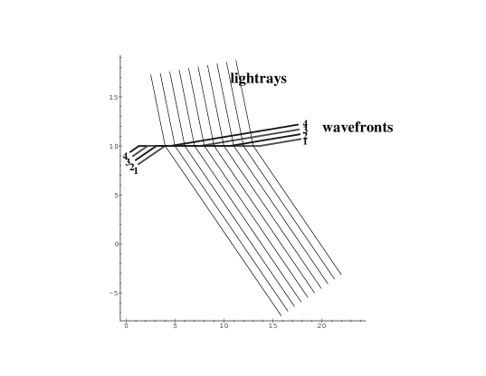
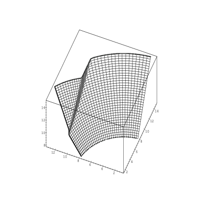
FIG. 2.: Envelope construction for the case of a bending angle independent of the location on the lens line $x_{l}$. The top panel shows a spacetime picture of one member of the 1-parameter family of null surfaces that is used to construct the envelope. The center panel is a space picture of the null surface, where both the lightrays and the associated wavefronts are shown. The bottom panel shows a spacetime picture of the envelope of the 1-parameter family. The family is labeled by the direction of the plane wave that hits the lens line.

FIG. 3.: Envelope construction for the case of a time delay $T(x_{l})=T_{0}-\ln(1+(x_{l}/x_{0})^{2})$. The top panel shows a space projection of one member of the family of null surfaces. The null surfaces are labeled by the direction of the plane that hits the lens line. The center panel contains a space picture of the envelope showing the lightrays. Notice the caustic line that develops after the lightrays pass through the lens line. The bottom panel shows a greatly magnified view of a few of the wavefronts associated with the lightrays of the center panel. Notice the cusp in each wavefront. These wavefronts occur around the value 20 in the verical axis of the center panel.

REFERENCES

- [1] P. Schneider, J. Ehlers and E.E. Falco, Gravitational Lenses (Springer-Verlag, New York, Berlin, Heidelberg, 1992)
- [2] V. Perlick, Ray Optics, Fermat’s Principle and Applications to General Relativity, (Springer-Verlag, Berlin, 2000)
- [3] A. O. Petters, H. Levine and J. Wambsganss, Singularity Theory and Gravitational Lensing, (Birkhauser, Boston, Baswel, Berlin, 2001)
- [4] S. Frittelli, G. Silva-Ortigoza, and E. T. Newman, J. Math Phys. 40, 383 (1999)
- [5] J. Ehlers and E.T. Newman, The Theory of Caustics and Wavefront Singularities with Physical Applications, J.Math.Phys., 41, 3344, (2000)
- [6] S. Frittelli and E. T. Newman, Phys.Rev. D, 59, 124001, (1999)
- [7] J. Ehlers, S. Frittelli and E.T. Newman, Graviational Lensing from a Space-Time Perspective, Boston Studies in the Philosophy of Science: Festschrift for John Stachel, edited by J. Renn (Kluwer Academic, Dordrecht, 2001)
- [8] See, for example, L. Landau and E. Lifschitz, The Classical Theory of Fields, (Addison-Wesley, Cambridge, Mass. 1951)
- [9] T. Pyne and M. Birkinshaw, ApJ 415, 459 (1993)
- [10] S. Capozziello, G. Lambiase, G. Papini and G. Scarpetta, Phys. Lett. A 254, 11 (1999)
- [11] T. Pyne and M. Birkinshaw, ApJ 458, 46 (1996)