The logic of causally closed space-time subsets

Abstract

The causal structure of space-time offers a natural notion of an opposite or orthogonal in the logical sense, where the opposite of a set is formed by all points non time-like related with it. We show that for a general space-time the algebra of subsets that arises from this negation operation is a complete orthomodular lattice, and thus has several of the properties characterizing the algebra of physical propositions in quantum mechanics. We think this lattice could be used to investigate the causal structure in an algebraic context. As a first step in this direction we show that the causal lattice is in addition atomic, find its atoms, and give necessary and sufficient conditions for ireducibility.

I Introduction

The logical propositions that represent physical questions in quantum mechanics are of the form ‘the state of the system is an eigenvector of the operator $\cal{O}$ with eigenvalue $\lambda$’, for an observable $\cal{O}$. The non commutativity of the observable operators gives place to a non Boolean logic for the propositions, in contrast to the case of the propositions about the phase space of a system in classical physics. This is mathematically described by the orthomodular lattice structure of projectors in Hilbert space, which is often called quantum logic [1, 2].

The algebra of propositions about the space in classical physics is Boolean. Consider for example a particle, and the set of propositions of the form ‘the particle is in the set $S$’. The opposite in this logic to the proposition given by the subset $S$ of the space is given by $-S$, the set of all points that do not belong to $S$. A positive answer to $S$ implies a negative one to $-S$. The intersection and union of sets corresponds to the conjunction and disjunction of logical propositions about the physical system. The algebra of propositions becomes the same as the Boolean algebra of subsets of the space in set theory. This structure is inherent to the space, because it will be the same for any system.

However, as we will see in the following, the situation when including time is different. In the relativistic context the kinematics imposed by the causal structure will induce a non Boolean character for the algebra of propositions given by certain space-time subsets (see [3] for the case of Galilean physics). A particle can not be concentrated at a given point $p$ in space-time because it existed in the past and will exist in the future of $p$, but we can think that the answer to the proposition given by a point is true if the particle passes through $p$ and false if not. The causal structure gives a definite prescription of what the opposite means in this case, because if the particle passes through $p$ it can not pass through any point spatially separated from $p$. All the points non related by a time-like curve to a given set $S$ will form the causal and logical complement of $S$.

A surprising fact about the algebra of propositions that arises along this line of thought from the causal structure of space-time alone, independently of the propagating physical system, is that it is also an orthomodular lattice. Though, we think, not widely known, this very interesting point was shown for Minkowski space some time ago in ref.[4].

In this work we will show how to define the lattice of causally closed sets ${\cal L}({\cal M})$ for a general space-time ${\cal M}$, even non causally well behaved, and prove that it is a complete orthomodular lattice. In addition, we will show that the lattice is atomic, and find its atoms. They are the points for causally well behaved space-times, but in general they can be of three different kinds. We will also find the necessary and sufficient conditions for this lattice to be irreducible.

The lattice ${\cal L}({\cal M})$ can have interest in two senses. We think that this lattice structure can be more fundamental than the causal structure of the space-time, much in the spirit of the studies of the postulates of quantum mechanics from the lattice perspective [2]. In this sense this paper can be consider as a step in the study of the causal structure of space-times from an algebraic point of view. In fact, we find that certain undesirable aspects of the causal structure of general space-times as closed time-like curves can be eliminated or localized in the structure of ${\cal L}({\cal M})$, this lattice being largely independent of the details of the metric in the bad sectors of space-time. Two space-times related by a conformal transformation will have the same causal structure and lattice ${\cal L}({\cal M})$, however the converse can be false.

The other aspect of interest is the possible relation of ${\cal L}({\cal M})$ with quantum mechanics and quantum field theory, motivated by the intriguing fact that causal structure and Hilbert space share an important piece of its mathematical structure. We will not develop in this sense here. We note, however, that the causally closed sets in ${\cal L}({\cal M})$ appear naturally in the algebraic approach to quantum field theory. In that context, we have a set of $C^{*}$-algebras associated to space-time sets. To a set in ${\cal M}$ and its causal complement correspond two $C^{*}$-algebras that commute. However, the whole relation between the lattice structure and the operations among local algebras seems not to be completely clear at the moment [5]. We will say a bit more in Section III.

To make this article as much self contained as possible, in the following Section we include a brief introduction to orthomodular lattices and some relevant mathematical preliminaries. Further details can be found in refs. [2, 6, 7]. In Section III we define the orthocomplemented complete lattice ${\cal L}({\cal M})$ and discuss several related possibilities for constructing causal set lattices. In Section IV we show that ${\cal L}({\cal M})$ is orthomodular. In Section V we show that it is atomic and find the atoms, which are an important piece in the understanding of the general structure of the lattice that will allows us to characterize irreducibility. In the last Section we make some comments and discuss directions open to future work.

II Orthomodular lattices

The family of subsets ${\cal B}(U)$ of any set $U$ forms a Boolean algebra when considered with the relation of inclusion, and the operations of intersection, union, and complement (denoted $\subseteq$, $\cap$, $\cup$ and $-$ respectively). This is at the base of the relation between set theory and classical logic, where the propositions can be restated in terms of the subsets of a given set $U$ in set theory. To a given proposition ${\cal P}$ we assign a subset $S$ with the interpretation that an element belongs to $S$ if and only if it satisfies the proposition ${\cal P}$. Thus, the operations of implication, conjunction, disjunction, and negation between propositions are interpreted as the relation of inclusion, and the operations of intersection, union, and complement between subsets respectively.

In quantum mechanics the space of individuals is given by a Hilbert space ${\cal H}$. The corresponding propositions or questions that are answered with a yes or a no, are given by projection operators $P$, $P^{2}=P$. These operators must be observables, that is, auto-adjoint operators, $P=P^{\dagger}$, such that their domain is all ${\cal H}$, and in consequence they are also bounded. The projection operators are in one to one correspondence with the closed subspaces $V_{P}$ of ${\cal H}$, such that $P\left(\,V_{P}\right)=V$, and $P(V_{P}^{\perp})=0$. Here we use the notation $W^{\perp}$ for the subspace orthogonal to $W$, which is always closed.

The interpretation is that the proposition $P$ is true for the elements of $V_{P}$ and false for the elements of $V_{P}^{\perp}$. Here is possible to talk in terms of propositions (projection operators) or in terms of closed linear subspaces indistinctly, as it happens in the case of classical logic, where it is possible to talk in terms of propositions or in terms of sets.

The set ${\cal C}({\cal H})$ of closed subspaces of a Hilbert space can be furnished with a structure that resembles the one in ${\cal B}(U)$, where the relation of inclusion and the operation of intersection between linear subspaces are the set inclusion and intersection, but where the set complement is replaced by the operation of taking the orthogonal subspace, and the union of two sets by the sum of subspaces. The resulting structure is called an orthomodular lattice. In what follows we will describe this structure in detail.

The inclusion between subsets is an order relation, that makes ${\cal C}({\cal H})$ (and ${\cal B}(U)$) a partially order set (poset),

$$A \subseteq A\,,$$ (1)

$$A \subseteq B\,,\,B\subseteq C\Rightarrow A\subseteq C\,,$$ (2)

$$A \subseteq B,\,B\subseteq A\Rightarrow A=B\,.$$ (3)

In ${\cal C}({\cal H})$ or ${\cal B}(U)$ there always exist elements that are the greatest lower bound (g.l.b.) and the lowest upper bound (l.u.b) of two given elements with respect to the order relation given by $\subseteq$. In ${\cal B}(U)$ they are given by the set intersection and union while in ${\cal C}({\cal H})$ by the set intersection and sum of linear subspaces. We will denote generically the g.l.b. and l.u.b. of two elements $A$ and $B$ as $A\wedge B$, and $A\vee B$ respectively, and call them the meet and the join of $A$ and $B$.

The meet and the join are associative and symmetric. A poset where the join and the meet of any two elements always exist is called a lattice. A lattice is in addition complete if the meet and the join exist for arbitrary families of elements.

A lattice ${\cal L}$ have a unit $I$ and a zero element $O$ if $A\subseteq I$ and $O\subseteq A$ for every element $A\in{\cal L}$.

An element $A$ in a lattice has a complement $B$ if it is $A\wedge B=O$ and $A\vee B=I$. The lattice is called orthocomplemented (or ortholattice) if there exist a unary operation $\perp:{\cal L}\rightarrow{\cal L}$ that assigns to every element $A$ a complement $A^{\perp}$, and in addition

$$A = (A^{\perp})^{\perp}\,,$$ (4)

$$A \subseteq B\,\Rightarrow B^{\perp}\subseteq A^{\perp}\,.$$ (5)

In an orthocomplemented lattice it can be deduced that $(A\vee B)^{\perp}=A^{\perp}\wedge B^{\perp}$ and $(A\wedge B)^{\perp}=A^{\perp}\vee B^{\perp}$, what shows that the negation is a dual map with respect to the operations $\wedge$ and $\vee$.

Both, ${\cal B}(U)$ and ${\cal C}({\cal H})$ are complete and orthocomplemented. However, for the lattice ${\cal B}(U)$ holds the distributivity law

$$A\wedge(B\vee C)=(A\wedge B)\vee(A\wedge C)\,,$$ (6)

while it is easy to see that it does not hold for ${\cal C}({\cal H})$. An orthocomplemented distributive lattice is called a Boolean algebra. However, in the lattice ${\cal C}({\cal H})$ holds a relaxation of the distributivity, called orthomodularity

$$B\subseteq A\,,\,C\subseteq A^{\perp}\Rightarrow\,A\wedge(B\vee C)=(A\wedge B)\vee(A\wedge C)\,.$$ (7)

Orthomodularity is equivalent to the simpler relation

$$B\subseteq A\Rightarrow\,A\wedge(B\vee A^{\perp})=B\,.$$ (8)

For finite dimensional Hilbert spaces a stronger form holds, the modular law,

$$B\subseteq A\,\Rightarrow\,A\wedge(B\vee C)=(A\wedge B)\vee(A\wedge C)\,,$$ (9)

whose definition, as the one of distributivity, makes no use of the orthocomplementation operation. Distributivity implies modularity and, for an orthocomplemented lattice, modularity implies orthomodularity.

We see that the orthomodular law (7) means that distributivity holds under special circumstances for the elements involved. In the lattice of closed linear subspaces of the Hilbert space, ${\cal C}({\cal H})$, when using the representation of projection operators, these conditions can be rewritten as that the projector $P_{A}$ commutes with $P_{B}$ and $P_{C}$. In a general orthocomplemented lattice two elements $A$ and $B$ are said to commute if

$$A{\sl=(}A\wedge B{\sl)\vee(A\wedge B}^{\perp}{\sl)\,}.$$ (10)

The relation of commutativity is symmetric in orthomodular lattices, and the Boolean subalgebras are formed by mutually commuting elements.

We will need a few additional definitions. With two lattices ${\cal L}_{1}$ and ${\cal L}_{2}$ we can construct the direct product of lattices ${\cal L}_{1}\times{\cal L}_{2}$ defined in the Cartesian product of sets, and where the operations are done component by component. The product of orthomodular lattices is orthomodular. A lattice is irreducible if it can not be written as a direct product of lattices. An orthocomplemented lattice is irreducible if and only if its centre, that is, the set of elements that commute with all other elements, is equal to $\{I,\,O\}$.

An atom of a lattice is a non zero element $A$ such that $A$ and $O$ are the only elements included in $A$. A lattice is atomic if every non zero element contains an atom. An orthomodular atomic lattice is also atomistic, that is, every non zero element is the join of the atoms that contains. Both, ${\cal B}(U)$ and ${\cal C}({\cal H})$ are atomic, its atoms being the points in $U$ and the unidimensional vector spaces in ${\cal H}$.

Closure and Galois connection

We will now describe a fundamental method for constructing complete orthocomplemented lattices that will be useful later [6]. The orthocomplemented lattice will be constructed with a subset (not a sublattice) of a given complete lattice ${\cal L}$ (not necessarily orthocomplemented). The idea is to start with a would be complement operation $\perp$ and then to require the elements in the new lattice to be the $A\in{\cal L}$ that satisfy $\perp\perp A=A$. This is imposed by eq.(4). This is similar to the case of a Hilbert space, where, if we start with ${\cal B}({\cal H})$ and propose the orthogonal to be the orthocomplement operation, the resulting lattice is ${\cal C}({\cal H})$, because the orthogonal of every set of vectors is a closed linear subspace.

Given a complete lattice ${\cal L}$ a Galois connection in ${\cal L}$ is a unary operation $g$ in ${\cal L}$ such that

$$X \subseteq Y\Rightarrow Y^{g}\subseteq X^{g}\,,$$ (11)

$$X \subseteq X^{gg}\,.$$ (12)

The operation $c=g\circ g$ is called a closure operation, and the elements $A$ of ${\cal L}$ that satisfy $A=A^{c}$ are called closed with respect to the closure operation $c$. The closure $c$ has the following properties

$$X \subseteq X^{c}\,,$$ (13)

$$X^{c} = X^{cc}\,,$$ (14)

$$X \subseteq Y\Rightarrow X^{c}\subseteq Y^{c}\,.$$ (15)

If we want the Galois connection $g$ to be an orthocomplementation we must pick up the elements of the lattice such that the closure operation is the identity operator in them, as is enforced by eq.(4). Indeed, if we further have

$$X\wedge X^{g} = O\,,$$ (16)

$$O^{g} = I\,,$$ (17)

the set of closed elements ${\cal L}^{c}$ of ${\cal L}$ with respect to $c$, forms a complete orthocomplemented lattice where the order and the meet are the order and the meet in ${\cal L}$, the complement is given by $g$ and the join is the join in ${\cal L}$ followed by the operation of closure $c$.

Finally, we add that there is a very natural way to construct a Galois connection in the lattice ${\cal B}(U)$. Let $R$ be a symmetric reflexive relation between points in the set $U$, with no further requirements. Thus $pRq\Leftrightarrow qRp$ and $pRp$. The operation $\perp:X\rightarrow X^{\perp}$ given by

$$X^{\perp}=\{q\,/\,-(qRp)\,\,\,\,\forall p\in X\}\,,$$ (18)

that is, the set of all points not related by $R$ with no point of $X$, is a Galois connection that satisfies eqs.(11, 12) and (16, 17).

III Causal set lattices

The space-time we will consider is a (Hausdorff) manifold ${\cal M}$ of dimension $d\geq 2$ with a pseudometric tensor $g_{\mu\nu}$ with signature $(+,-,..,-)$, smooth and non singular everywhere. We do not ask the space-time ${\cal M}$ to be time orientable nor to satisfy any causality condition (for example to be free from closed time-like curves). For a review of causal structure see refs. [8, 9, 10]. Given a definite naming of the local light cones of a point $p$ as future and past light cones, its causal future and past, $I^{+}(p)$ and $I^{-}(p)$, are defined as the set of points that can be reached by time-like curves starting at $p$ with tangent vector in the future and past light cone of $p$ respectively. When referring to time-like curves we always mean differentiable curves with continuous tangent vector except a finite number of points where the tangent can have a discontinuity, but keeping always in the same local light cone. These discontinuities can always be removed by modifications in arbitrarily small neighborhoods. The past and future of $p$ are open sets. We will use the symbol $I^{+}(S)\cup I^{-}(S)$ for the open set $\bigcup\limits_{q\in S}(I^{+}(q)\cup I^{-}(q))$ that always makes sense, even in non time-orientable space-times.

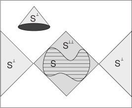
FIG. 1.: The orthocomplement $S^{\perp}$, and the set generated $S^{\perp\perp}$ by a given set $S$. The space-time is the two-dimensional Minkowski space where we have taken out the closed set shown in black. Both, $S^{\perp}$ and $S^{\perp\perp}$ are in ${\cal L(M)}$, while $S$ is not. Note that in this example all points in the border of $S^{\perp}$ are in $S^{\perp}$ while all points in the border of $S^{\perp\perp}$, except the ones at the spatial corner, are in $S^{\perp\perp}$.

The natural orhtocomplement operation for sets in ${\cal M}$ based on the causal structure identifies all that is not time-like related to a given set with its complement. To be explicit, we can define in ${\cal M}$ a symmetric reflexive relation that relies only on the causal structure. Given two points $p$ and $q$ of ${\cal M}$ we write $p\sim q$, and say that $p$ and $q$ are time-connected or just connected, if there is time-like curve that passes through $p$ and $q$. Thus, $p\sim q$ is equivalent to $p\in I^{+}(q)\cup I^{-}(q)\cup\{q\}$. All points that are not time-connected to $p$ must be in the complement of $p$. Starting from this complement operation, as it was described in the previous Section, we can construct a complete orthocomplemented lattice coming from the Galois connection in ${\cal B}({\cal M})$ given by eq.(18). We call it the lattice of the causally closed sets ${\cal L}({\cal M})$. The orthocomplement is given by

$$S^{\perp}=\{p\,/\,p\text{ is not time-connected to any point of }S\}=-\left(S\cup I^{+}(S)\cup I^{-}(S)\right)\,,$$ (19)

and, $S\in{\cal L}({\cal M})$ if and only if $S^{\perp\perp}=S$. The fig. 1 shows an example of $S^{\perp}$ and $S^{\perp\perp}$ for a set $S\subseteq{\cal M}$. An important property to keep in mind is that, for every set $S$, the opposite $S^{\perp}$ is already an element of ${\cal L}({\cal M})$, because $S^{\perp}=S^{\perp\perp\perp}$.

A typical element $S$ of ${\cal L}({\cal M})$ in Minkowski space is a diamond shaped set, with the upper and lower cone being null surfaces included in $S$, while the points in the spatial corner may or may not be in $S$. However, in Minkowski space many other sets, including lower dimensional objects, are in the lattice. The bounded null surfaces of dimension $d-1$ or lower are sets in ${\cal L}({\cal M})$ while space-like surfaces of dimension $d-2$ or less are in ${\cal L}({\cal M})$, while spatial surfaces of dimension $d-1$ are not. On the other hand every set with at least two different points time-like connected will generate a set that contains an open set in ${\cal M}$. The sets generated by subsets in achronal surfaces form Boolean subalgebras.

The meet in ${\cal L}({\cal M})$ is just the set intersection. The join of a family of elements is given by the set union followed by the causal closure (the double orthogonal)

$$\bigvee_{x\in F}A_{x}=\left(\bigcup_{x\in F}A_{x}\right)^{\perp\perp}\,.$$ (20)

The join of two sets is exemplified in fig. 2. For two spatially separated sets $A$ and $B$ the set $A\vee B$ will be just the set union $A\cup B$, while otherwise $A\vee B$ will contain also at least all the time-like curves that connect points from $A$ to $B$. In general, for a set $A$ in ${\cal M}$, the causal closure $A^{\perp\perp}$ is bigger than the domain of dependence of $A$, taking this latter as the set of points such that all past (future) inextendible time-like curves from the point intersects the given set [9] (see fig. 2).

The lattice ${\cal L}({\cal M})$ is not distributive nor modular in the general case, as it is shown for Minkowski space in fig. 3(a) and fig.3(b), while it is orthomodular as will be shown in the next Section and is illustrated in fig. 3(c).

As mentioned in the Introduction, the lattice ${\cal L}({\cal M})$ has a logical interpretation in terms of propositions for classical particles. The proposition corresponding to a space-time subset $S$ is given by “the particle passes through S”. However, for an arbitrarily chosen set $S$ the logical opposite of that proposition is “the particle does not passes through $S$”. In general this is not of the form “the particle passes through $T$” for some space-time subset $T$. The prescription of taking causally closed sets is just what is needed to have a closed algebra of propositions coming from space-time subsets in the above sense. In contrast to the case of the Boolean logic of space subsets, here only some subsets of space-time have an opposite in terms of space-time subsets, and the resulting algebra is non Boolean. The logical interpretation of the operation $\wedge$ between two propositions corresponding to the sets $A$ and $B$ is given by the maximal space-time proposition that implies “the particle passes through $A$ and $B$”, while the proposition corresponding to $A\vee B$ is given by the minimal space-time proposition implied by “ the particle passes through $A$ or $B$”.

It is immediate that when the manifold ${\cal M}$ is non connected the lattice ${\cal L}({\cal M})$ is the direct product of the lattices ${\cal L}({\cal M}_{i})$ of each connected component ${\cal M}_{i}$ of ${\cal M}$. In this case the lattice is reducible. We will see a sufficient condition for irreducibility in Section V.

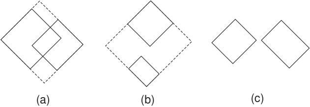
FIG. 2.: Three cases for the join of two sets in two-dimensional Minkowski space. The set formed by the join is shown with dashed lines. In case (a) the join is equal to the domain of dependence of the set union, while in case (b) it is not. The case (c) shows the join of two spatially separated sets, that coincides with the set union.

One can try to construct other lattices based on the causal structure of ${\cal M}$. For example, the basic symmetric and reflexive relation between points used to define the orthocomplement can be taken as the relation $pSq$, that holds if there is a space-like curve passing through $p$ and $q$, or $pCq$, that holds if there is a causal curve (i.e. a curve with time-like or null tangent) passing through $p$ and $q$, or $pNq$, that holds if there is null curve passing through $p$ and $q$, or several logical combinations between them (no discontinuities are allowed in the tangent to null and causal curves). Accordingly, three orthocomplemented and complete lattices can be constructed, ${\cal L}_{S}({\cal M})$, ${\cal L}_{C}({\cal M})$ and ${\cal L}_{N}({\cal M})$ respectively. The lattice ${\cal L}_{S}({\cal M})$ is trivial when $d\geq 3$ because a space-like curve from a point can get inside the light cone, while in two dimensions it does not add anything new to ${\cal L}({\cal M})$. The same triviality will occur in ${\cal L}({\cal M})$ if the metric would have more than one time directions. It is easy to see that ${\cal L}_{C}({\cal M})$ and ${\cal L}_{N}({\cal M})$ fail to be orthomodular in the simplest case of Minkowski space. It seems that in the case of ${\cal L}_{N}({\cal M})$ it is not possible to change slightly the definition of the lattice to make it orthomodular. The lattice ${\cal L}_{C}({\cal M})$ differs from ${\cal L}({\cal M})$ fundamentally in details of the borders of the sets, what is crucial for orthomodularity. Other logical combinations seem to lead to the same lattices or to uninteresting and trivial cases.

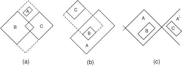
FIG. 3.: Examples in two dimensional minkowski space. (a) Distributivity does not hold. We see that $A\wedge B=A\wedge C=O$, but $A\wedge(B\vee C)=A$. (b) The modular law does not hold. It is $B\subseteq A$, however $A\wedge(B\vee C)$ is greater than $(A\wedge B)\vee(A\wedge C)=B$. (c) Orthomodularity holds. Under the conditions $B\subseteq A$, $C$ $\subseteq A^{\perp}$, the distributivity $A\wedge(B\vee C)=(A\wedge B)\vee(A\wedge C)=B$ holds.

One may wonder if there is another way for constructing a causal lattice that yielding open sets or sets with better topological properties. A lattice of open sets can be constructed using the complete lattice ${\cal O}({\cal M})$ of open sets in ${\cal M}$ as a base where to define the Galois connection [6]. The join in ${\cal O}({\cal M})$ is the usual set union and the meet of arbitrary families of open sets is given by the set intersection followed by the operation of interior. Then we define $S^{\perp}$ for an open $S$ as

$$S^{\perp}=-(\overline{I^{+}(S)\cup I^{-}(S)})\,,$$ (21)

where here $\overline{A}$ means the usual topological closure of $A$. This satisfies eqs.(11, 12) and (16, 17), and lead to a complete orthocomplemented lattice ${\cal L}_{{\cal O}}({\cal M})$ of open sets. However, again due to details in the borders of the sets, the lattice is not orthomodular, as is shown in fig. 4. It can be shown, at least for globally hyperbolic space-times, that distributivity in ${\cal L}_{{\cal O}}({\cal M})$ holds under a little more stringent conditions than the required by orthomodularity. In fact, instead of eq.(8) we have

$$\overline{B}\subseteq A\Rightarrow\,A\wedge(B\vee A^{\perp})=B\,.$$ (22)

It seems essential for orthomodularity that the lattice should contain along with the diamond shaped sets at least the null surfaces. Once we have null surfaces in the lattice its intersection will generate lower dimensional sets as lines and points.

This makes difficult a correspondence between the elements in an orthomodular lattice of causal sets with $C^{*}$-algebras in the algebraic approach to quantum field theory, because the points should be assigned non trivial algebras (two points can generate a set that includes an open set) (see the discussion in [5]). The lattice ${\cal L}_{{\cal O}}({\cal M})$ would be a better candidate, but it is only approximately orthomodular in the sense of eq.(22) (weaker conditions for distributivity can also be found).

Form now on we will only refer to ${\cal L}({\cal M})$. From its definition we see that it does not change with conformal transformations, and thus it is a property of the conformal structure.

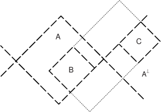
FIG. 4.: Orthomodularity does not hold for ${\cal L}_{{\cal O}}({\cal M})$. All sets are open. The sets $B\subseteq A$ and $C\subseteq A^{\perp}$ share sectors of the border with $A$ and $A^{\perp}$ respectively. The set $B\vee C$ is shown with short dashed lines. The lack of orthomodularity can be traced back to the absence of the null surface joining $B$ and $C$ in the orthogonal sets $B^{\perp}$ and $C^{\perp}$

IV Orthomodularity of ${\cal L}({\cal M})$

We will now prove that ${\cal L}({\cal M})$ is orthomodular in any space-time. First, we will prove the following previous result.

Lemma 1: Given a time-like curve $\gamma(x)$ parametrized by a real variable $x$ in a closed interval $x\in[a,b]$ and a set $S\in{\cal L}({\cal M})$, the intersection $\gamma([a,b])\cap S$ is empty or it is a closed segment of $\gamma$, corresponding to $x\in[c,d]\subseteq[a,b]$.

Suppose $x_{1}\in[a,b]$ and $x_{2}\in[a,b]$, with $x_{1}\leq x_{2}$ are such $\gamma(x_{1})\in S$ and $\gamma(x_{2})\in S$, then it is $\gamma([x_{1},x_{2}])\subseteq S$. Otherwise, if $y\in[x_{1},x_{2}]$ is such that $\gamma(y)$ is not in $S$, it can be connected by a time-like curve to $S^{\perp}$ (if not it would be in $(S^{\perp})^{\perp}=S$), and thus either $\gamma(x_{1})$ or $\gamma(x_{2})$ is connected by a time-like curve to $S^{\perp}$, contradicting the assumptions. Then, if the intersection $\gamma([a,b])\cap S$ is non empty, let $c$ and $d$ be the infimum and supremum of the points $x$ in $[a,b]$ such that $\gamma(x)\in S$. The point $\gamma(c)$ is connected with $S$ so $\gamma(c)\notin$ $S^{\perp}$, then if $\gamma(c)\notin S$ it is connected also with $S^{\perp}$, and thus belong to the open set $I^{+}(S^{\perp})\cup I^{-}(S^{\perp})$. A neighborhood of $\gamma(c)$ will belong to $I^{+}(S^{\perp})\cup I^{-}(S^{\perp})$ and will not be in $S$, what is not possible, so $\gamma(c)\in S$. Similarly we have $\gamma(d)\in S$.

Therefore, a set $S$ in ${\cal L}({\cal M})$ contains all time-like segments between points in $S$ and also the time-like border of $S$, that is, the border of $S$ accessible from $S$ by time-like curves. The points in the space-like border of $S$ may or may not belong to $S$. Using Lemma 1 we prove

Theorem 1: ${\cal L}({\cal M})$ is orthomodular

Orthomodularity is the implication $B\subseteq A\Rightarrow A\wedge(B\vee A^{\perp})=B$ for any $A$ and $B$ in ${\cal L}({\cal M})$. If the set $B$ is included in $A$ it is also included in $A\wedge(B\vee A^{\perp})$. Then we have to show that $B\subseteq A\Rightarrow A\wedge(B\vee A^{\perp})\subseteq B$. To start we assume that $B\subseteq A$. Let $p\in A\wedge(B\vee A^{\perp})$, so $p\in A$ and $p\in B\vee A^{\perp}$. Therefore no time-like curve connects $p$ with $A^{\perp}$ nor with $B^{\perp}\wedge A$. We have to prove that $p\in B$. Then, let us suppose that $p\notin B$ and show that it leads to a contradiction. This assumption implies that there is a time-like curve $\gamma$ that connects $p$ with a point $q\in B^{\perp}$. As $p$ is not connected with $A^{\perp}$ nor with $B^{\perp}\wedge A$ it is $q\notin A$ and $q\notin A^{\perp}$. A segment of $\gamma$ with end points $p$ and $q$ intersects $B^{\perp}$ and $A$ in non empty sets, which according to Lemma 1 are closed segments. These are disjoint, because otherwise $p$ could be connected with a point in $B^{\perp}\wedge A$. Thus, there is a point $r$ in the segment of $\gamma$ between $p$ and $q$ that is not in $B^{\perp}$ nor in $A$. As $r\notin B^{\perp}$, $r$ can be connected with a point $s\in B$. Thus, as $r$ is in the segment of $\gamma$ between $p$ and $q$ it is either $q$ connected with $s$ or $p$ connected with $s$. However, the point $q\in B^{\perp}$ can not be connected with $s\in B$. Then $p\in A$ is connected with $s\in B\subseteq A$ by a curve passing through $r$. Then, by Lemma 1, it is $r\in A$, what shows a contradiction. Therefore $p\in B$ and orthomodularity holds.

Of course, there are orthomodular lattices that are not of the form ${\cal L}({\cal M})$ for a space-time ${\cal M}$. In the following Section we go a step further in the characterization of causal structures from the lattice theoretical point of view by showing that ${\cal L}({\cal M})$ is atomic, and finding its atoms. In the remaining part of this Section we will extract what are the essential properties of the causal structure used in the proof of orthomodularity (see ref.[11] for a related discussion).

For constructing an orthocomplemented lattice we used a symmetric reflexive relation between points in the space-time with no further properties. Now we can read from the previous theorem what additional structure of the causal relation $\sim$ that we used in the definition of ${\cal L}({\cal M})$ is central in the proof of orthomodularity. Basically, what we need is a set of curves in a set ${\cal M}$, locally one to one functions of (possible infinite) open intervals of real numbers to ${\cal M}$, that we can call time-like curves. Given a point $p$ and any curve $\gamma$ with $\gamma(x)=p$, the points $\gamma(y)$ with $y\neq x$ belong to two sets, non necessarily disjoint, that we can call the past and future sets of $p$. We have either all $\gamma(y)$ for $y>x$ belong to the future of $p$ and all $\gamma(y)$ for $y<x$ belong to the past of $p$ or vice versa. If a point $q$ is in the future set of $p$, then either all the future set of $q$ or the past set of $q$ are included in the future set of $p$, and, in addition, there is a neighborhood of $q$ (in the sense induced by the real numbers) in all time-like curves passing through $q$ that belongs to the future set of $p$. The same can be said regarding the past set of $p$.

These geometrical properties, that are immediate for the time-like curves in a general space-time ${\cal M}$, are sufficient in order to have an orthomodular lattice generated by the relation $\sim$. We see that certain sort of transitivity condition is essential for the causal relation but, for non orientable space-times no global transitive relation can be defined. There is also a condition of continuity. None of these is respected by the relation $N$ defined in the preceding Section, while the relation $C$ does not respect the continuity condition.

V Atoms

An atom $S$ in ${\cal L}({\cal M)}$ must be equal to the set $p^{\perp\perp}$ generated by any point $p\in S$, because $p^{\perp\perp}$ is a non empty element of ${\cal L}({\cal M})$ included in $S$. Therefore, all atoms are of the form $p^{\perp\perp}$ for some point $p$, what shows what are the sets among which to look for atoms. However, the element $p^{\perp\perp}$ need not be an atom. By contrast, if $p$ as a subset of ${\cal M}$ is an element of ${\cal L}({\cal M)}$, $p^{\perp\perp}=p$, then it is an atom. This is the case for all points in Minkowski space. We will now analyze which of the points of ${\cal M}$ are atoms in the general case.

As we noted before, if two points $p$ and $q$ belong to $S$ in ${\cal L}({\cal M)}$, then all points in time-like curves connecting $p$ and $q$ are also in $S$. If there is a time-like segment $\gamma$ connecting a point $p$ with itself, then $p$ can not be an atom because $\gamma\subseteq p^{\perp\perp}$. There are two types of such curves, as shown in fig. 5. One, the closed time-like curves, that are totally included in the intersection $I^{+}(p)\cap I^{-}(p)$, where a segment of the curve between $p$ and $p$ start and end with its tangent vector in the same light cone of $p$. The other type, that we will call vertex curves, where a segment between $p$ and $p$ start and end with tangent vectors at $p$ in different light cones of $p.$ In this later case we will call $p$ a vertex. For the existence of these types of curves the manifold must not be simply connected [10]. In the vertex curve case we see that the space-time is not time orientable. However, there are time non orientable space-times without vertex curves. The vertex curves mark space-times where the notion of future and past have no sense for a single observer. The points $p$ that belong to closed time-like curves or are vertex points can be characterized as all points that belong to $I^{+}(q)\cap I^{-}(q)$ for some $q$ of ${\cal M}$ (any $q$ of $\gamma$ in the open segment between $p$ and $p$ for example). We will call it the set ${\cal B}$ of bad points of ${\cal M}$, ${\cal B}$ $=\cup_{q\in{\cal M}}I^{+}(q)\cap I^{-}(q)$. As union of open sets, ${\cal B}$ is also open.

The set of points in closed time-like curves ${\cal C}$, and the set of vertices ${\cal V}$, are also separately open, and by definition ${\cal B=C\cup V}$. To see this, let $p\in\gamma$, where $\gamma$ is a closed time-like curve, and take a sufficiently small, open, time orientable, normal neighborhood $U$ of $p$ [9]. Let $q$ and $r$ be two points of an interval of $\gamma$ included in $U$ that contains $p$, respectively in the future $I_{U}^{+}(p)$ and past $I_{U}^{-}(p)$ of $p$, where $I_{U}^{+}$ and $I_{U}^{-}$ are the notions of future and past in the submanifold $U$. Doing a composition with the curve $\gamma$, we have that all points in the open neighborhood $I_{U}^{-}(q)\cap I_{U}^{+}(r)$ of $p$ are connected by a closed time-like curve to every point in $\gamma$. Thus, the set of points connected by closed time-like curves to a point $p$ form an open subset ${\cal C}_{p}$ of ${\cal C}$. It is immediate that the sets of the form ${\cal C}_{p}$ are either disjoint or identical, so ${\cal C}$ is the union of disjoint sets of the form ${\cal C}_{p}$. Note that for any time-like curve $\delta$ that passes through $p$ we have that there is an open interval around $p$ in $\delta$ that is included in a closed time-like curve trough $p$. The proof that ${\cal V}$ is open can be done similarly.

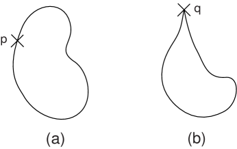
FIG. 5.: (a) A closed time-like curve. All points in the curve are in the past and the future of all points in the curve. (b) A vertex curve with vertex point $q$. The vertex is in the past and the future of all points in the vertex curve (except $q$).

The following Lemma solves the question of when a point in ${\cal M}$ is an element, and therefore an atom, in ${\cal L}({\cal M})$

Lemma 2: the set formed by a point $p$ in ${\cal M}$ is an element and an atom in ${\cal L}({\cal M})$ if and only if $p\notin{\cal B}$

As we have seen if $p\in{\cal B}$ the set formed by $p$ is not an element of ${\cal L}({\cal M})$ and can not be an atom. We will show that if $p$ is not an atom then $p\in{\cal B}$. Let us suppose $p^{\perp\perp}\neq p$. Thus, there is a point $q\in p^{\perp\perp}$ with $q\neq p$. The point $q$ must be time connected with $p$ otherwise it would be $q\in p^{\perp}$. Therefore $p\in I^{+}(q)\cup I^{-}(q)$ and a connected, time orientable, open neighborhood $U$ of $p$ is included in $I^{+}(q)\cup I^{-}(q)$. Thus, as every point in $U$ is connected with $q\in p^{\perp\perp}$, it must be that $U\cap p^{\perp}$ is empty. In other words $p^{\perp}$ is separated from $p$. Then all points $r$ in the open connected set $U-\{p\}$ are in $I^{+}(p)$ or in $I^{-}(p)$. With a given continuous time orientation in $U$ we have for every $r\in U-\{p\}$ that $p$ is in $I^{+}(r)$ or in $I^{-}(r)$, and the sets $\{r\,/\,r\in(U-\{p\})\,,\,p\in I^{+}(r)\}\,$ and $\{r\,/\,r\in(U-\{p\})\,,\,p\in I^{-}(r)\}$ are open. They cover all the connected set $U-\{p\}$, and thus must have a non empty intersection, with a point $s$. Therefore $p$ belongs to $I^{+}(s)\cap I^{-}(s)$ and thus $p\in{\cal B}$.

We have shown that in the closed set ${\cal M-B}$ all points are atoms. Next we will show that a different kind of atoms can exist in space-times that have both types of defects, closed time-like and vertex curves. Consider the time-like curve $\beta$ of fig. 6. We will call such a curve a bridge. It is a closed time-like curve but also a past and future vertex curve for all points in the curve. The essential property of a bridge is that for any point $p$ in it one can construct a time-like curve that passes through $p$ with tangent in any light cone and passes through any point $q$ in the bridge with tangent in the any light cone of $q$. Thus any two points time connected with two points in the bridge $\beta$ are also connected to each other. Then we have the following

Lemma 3: the set $\beta^{\perp\perp}$ generated by any bridge $\beta$ is an atom

Let $p\in\beta$ (see fig. 6). If $q\in p^{\perp\perp}$ then $q$ is connected with $p$. The set $q^{\perp\perp}$ is included in $p^{\perp\perp}$ and if they are different it must be $p\notin q^{\perp\perp}$. In that case $p$ must be connected with $q^{\perp}$. But that is not possible because as $p$ belongs to a bridge it would lead to $q$ connected with $q^{\perp}$. Thus $q^{\perp\perp}=p^{\perp\perp}$ for every $q\in p^{\perp\perp}$ and $p^{\perp\perp}$ is an atom that includes $\beta$.

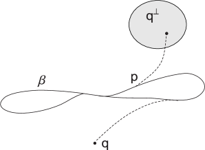
FIG. 6.: A bridge time-like curve $\beta$. If a point $q$ is in $\beta^{\perp\perp}$ it must be connected with $\beta$. A point in $q^{\perp}$ can not be connected with a point $p$ in $\beta$, otherwise it would be connected with $q$. Thus, $\beta$ is in $q^{\perp\perp}$. Note that every two points in $\beta$ can be connected by a time-like curve (based on $\beta$) with tangent in any light cone of the points. This does not happen for simple closed time-like curves or vertex curves.

We will call the set $\beta^{\perp\perp}$ generated by a bridge $\beta$ a bridge atom. Any bridge atom contains an open set. We also have that two atoms cannot intersect. Therefore in a paracompact manifold there can be at most a numerable amount of bridge atoms. The bridge atoms must be totally included in the set of bad points ${\cal B}$.

We have shown what happens to the sets $p^{\perp\perp}$ for $p\in{\cal M-B}$ or $p$ in $\beta^{\perp\perp}$ where $\beta$ is a bridge. In both cases $p^{\perp\perp}$ is an atom. We will see that this is not always the case. First consider the case where $p$ is a vertex. We have

Lemma 4: The set $p^{\perp\perp}$ where $p$ is a vertex contains a point in ${\cal M-B}$ or a bridge atom

Let $\gamma(z)$, $z\in[0,1]$, and $\gamma(0)=\gamma(1)=p$ be a vertex curve of the vertex $p$. Let us suppose that every point in $\gamma$ is in ${\cal B}$. For every value of the parameter $z\in[0,1]$ we define the future light cone of $\gamma(z)$ at $z$ as the light cone of $\gamma(z)$ given by the tangent vector of $\gamma$ at $z$. Thus, the direction of the tangent vector at the point $z=1$ will mark the future light cone of $p$ at $z=1$, but it will be a different light cone of the point $p$ than the future light cone at $z=0$. For any $z$ such that the point $q=\gamma(z)$ is a vertex, we can define it as a future or a past vertex according the vertex curve based at $q$ starts with tangent in the future or the past light cone of $q$ at $z$. Let us call $W^{+}\subseteq[0,1]$ and $W^{-}\subseteq[0,1]$ the set of values of the parameter that have future and past vertices respectively. These sets are non empty as $0$ has a future vertex and $1$ has a past vertex. If $w_{1}$ has a past vertex and $w_{2}$ has a future vertex and $w_{1}\leq w_{2}$, then both vertex curves together with $\gamma([w_{1},w_{2}])$ will form a bridge. Let the infimum of $W^{-}$ be $w^{-}$ and the supremum of $W^{+}$ be $w^{+}$, and assume $w^{+}\leq w^{-}$. The points in $\gamma([w^{+},w^{-}])$ must belong to closed time-like curves, $\gamma([w^{+},w^{-}])\subseteq{\cal C}$ (the points $w^{+}$ and $w^{-}$ can not be vertices as ${\cal V}$ is open). But as ${\cal C}$ is open there must be $x^{+}$ and $x^{-}$ with $x^{+}<w^{+}\leq w^{-}<x^{-}$ and such $\gamma([x^{+},x^{-}])\subseteq{\cal C}$. For each $y\in[x^{+},x^{-}]$ let $I_{\gamma(y)}$ be an open interval of $\gamma$ around the point $\gamma(y)$ that is included in a closed time-like curve through $\gamma(y)$. The sets $[x^{+},x^{-}]\cap\gamma^{-1}(I_{\gamma(y)})$ are open in the topology of the interval, and cover the compact $[x^{+},x^{-}]$. After extracting a finite covering and gluing together a finite number of closed curves, we have that $x^{+}$ and $x^{-}$ are connected by a closed time-like curve $\delta$ that includes $\gamma([x^{+},x^{-}])$. Then it is easy to see that the union of $\delta-\gamma([x^{+},x^{-}])$ with the vertices at $x^{+}$ and $x^{-}$ is a bridge.

Then let us consider now the case of points in closed time-like curves. Let $p$ be a point in ${\cal C}$ and ${\cal C}_{p}$ be the connected component of ${\cal C}$ that includes $p$. It is ${\cal C}_{p}\subseteq p^{\perp\perp}$. If ${\cal C}_{p}$ is a connected component of ${\cal M}$ then ${\cal C}_{p}$ will be an atom. If this is not the case, let $q$ be a point in the border of ${\cal C}_{p}$. The point $q$ can only be a vertex or a point in ${\cal M}-{\cal B}$. Therefore if $p^{\perp\perp}$ contains a point in the border of ${\cal C}_{p}$ it will contain an atom. But any point in the border of ${\cal C}_{p}$ that can be reached by a time-like curve passing through a point in $p^{\perp\perp}$ must belong to $p^{\perp\perp}$ because of Lemma 1. Thus, if there are no point or bridge atoms in $p^{\perp\perp}$ we have ${\cal C}_{p}=I^{+}({\cal C}_{p})\cup I^{-}({\cal C}_{p})$. A point in the set $-{\cal C}_{p}$ can not be joined by a time-like curve to ${\cal C}_{p}$, and, as every point is in the future or the past of a different point, it is $-{\cal C}_{p}=I^{+}(-{\cal C}_{p})\cup I^{-}(-{\cal C}_{p})$. Therefore ${\cal C}_{p}$ and $-{\cal C}_{p}$ are open disjoint sets that cover ${\cal M}$, and ${\cal C}_{p}$ is a connected component of ${\cal M}$.

Resuming, we have shown

Theorem 2: ${\cal L}({\cal M})$ is an atomic lattice. Its atoms are all the points in ${\cal M-B}$, the bridge atoms, and the connected components of ${\cal M}$ included in ${\cal C}$

Taking into account that ${\cal L}({\cal M})$ is orthomodular we also have,

Corollary: ${\cal L}({\cal M})$ is atomistic

That is, every element is the join of the atoms that includes. Thus, from the algebraic point of view all the bad points of the space-time disappear from the algebra, except the discrete bridge atoms and connected components included in ${\cal C}$ (see fig. 7). These later obviously commute with all ${\cal L}({\cal M})$ and then belong to the centre. We can see that the same is true for the bridge atoms as follows.

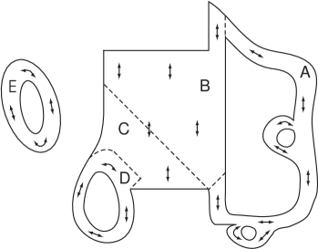
FIG. 7.: A two dimensional space-time showing the different kinds of atoms. The direction of the light cones is marked with double arrows. The set A is a bridge atom. The set B is formed by vertex points that generates a set containing the bridge atom. The closed set C is equal to ${\cal M-B}$, and all points in this set are atoms. The sets D and E are formed by closed time-like curves. While E is a connected component of ${\cal M}$, and hence an atom, D is not. The lattice ${\cal L}({\cal M})$ is generated by the points in C and the isolated atoms A and E. These later commute with all other elements. Note, however, that the lattice generated by ${\cal M-B}$ can not be deduced in general with the only knowledge of the space-time metric in ${\cal M-B}$.

Lemma 5: the bridge atoms belong to the centre of ${\cal L}({\cal M})$

If an atom does not belong to $\beta^{\perp}$ for a bridge $\beta$ it must be connected with $\beta$. If the atom is a point $p$ then as $p$ is connected with $\beta$ it implies that $p$ is a vertex, what is not consistent with $p$ being an atom. Then let the bridge $\chi$ be connected with $\beta$, it is easy to see that both will generate the same set, $\beta^{\perp\perp}=\chi^{\perp\perp}$ (they form a unique bridge curve). Thus an atom is either equal to $\beta^{\perp\perp}$ or is included in $\beta^{\perp}$, and therefore commutes with $\beta^{\perp\perp}$. As ${\cal L}({\cal M})$ is atomistic, and every element is the join of its atoms, $\beta^{\perp\perp}$ will commute with all the elements of the lattice [7].

We have shown that if the manifold is not connected or if it contains at least two atoms and a bridge then ${\cal L}({\cal M})$ is reducible. We will complete the following

Theorem 3: ${\cal L}({\cal M})$ is trivial (equal to $\{O,{\cal M}\}$) if and only if ${\cal M}=\beta^{\perp\perp}$ for a bridge $\beta$ or ${\cal M}$ is connected and ${\cal M}={\cal C}$. If non trivial, ${\cal L}({\cal M})$ is irreducible if and only if ${\cal M}$ is connected and does not contain any bridge curves

Assume that ${\cal M}$ does not have bridge curves, nor connected components includes in ${\cal C}$. Then, its only atoms are the points in ${\cal M-B}$. We can identify all the sets in ${\cal L}({\cal M})$ with the set of its atoms, $\hat{S}=S\cap({\cal M-B})$. Let now $S$ be a proper element in ${\cal L}({\cal M})$. If there is a point $p$ in ${\hat{\cal M}}-\hat{S}-\hat{S}^{\perp}$ it will be an atom that does not commute with $S$ (see eq.(10)). Thus, if $S$ is in the centre of ${\cal L}({\cal M})$, it must be ${\hat{\cal M}}=\hat{S}\cup\hat{S}^{\perp}$, and $\hat{S}\cap\hat{S}^{\perp}=\emptyset$. Let $q$ be a point in ${\cal M}$, then, as the atoms that generate $q^{\perp\perp}$ are in $S$ or in $S^{\perp}$, we have $q^{\perp\perp}=(q^{\perp\perp}\cap S)\vee(q^{\perp\perp}\cap S^{\perp})=(q^{\perp\perp}\cap S)\cup(q^{\perp\perp}\cap S^{\perp})$, the last equality coming from the form of the join for orthogonal sets. Thus, $q$ belongs to $S\cup S^{\perp}$, $S\cup S^{\perp}={\cal M}$, $S\cap S^{\perp}=O$. Then, all future and past of all points of $S$ must be in $S$, otherwise $S$ would be connected with $S^{\perp}$, and, as for a point $r$ $\in S$ there is always a different point $s$ in a neighborhood that is in $I^{+}(r)\cup I^{-}(r)$, and so $r$ $\in I^{+}(s)\cup I^{-}(s)$ with $s\in S$. Therefore $S=I^{+}(S)\cup I^{-}(S)$ is an open set. The same can be said for $S^{\perp}$, $S^{\perp}=I^{+}(S^{\perp})\cup I^{-}(S^{\perp})$. Therefore, ${\cal M}$ is non connected.

The case where ${\cal L}({\cal M})$ is nontrivial and irreducible is the most interesting for physical space-times. In that case there is a non countably number of atoms formed by the points in $\overline{{\cal M-B}}$, that can be consider the relevant space-time from the algebraic point of view.

VI Discussion

We have already mentioned that the lattice ${\cal C}({\cal H})$ of closed linear subspaces of the Hilbert space is complete, atomic, irreducible and orthomodular. It has a further property called the covering law. An element $A$ in a lattice is said to cover $B$ if $B\subseteq A$ and if for every element $C$ such that $B\subseteq C\subseteq A$ it is $C=A$ or $C=B$. The covering law means that given an atom $X$ and an element $A$ with $A\wedge X=O$, then $X\vee A$ covers $A$. There exist reconstruction theorems stating that a complete, atomic, irreducible, orthomodular lattice, satisfying the covering law, can be represented as a lattice of closed linear subspaces of a vector space with a Hermitian form [2]. Under minor assumptions regarding the field of scalars for the vector space it is the lattice of a Hilbert space. Thus, a lattice with this set of properties characterize almost uniquely Hilbert spaces.

FIG. 8.: The picture on the left shows a space-time constructed over a cylinder with no closed time-like curves but that is not strongly causal. This means that there is a point (all points in $B$) such that each of its neighborhoods is intersected by a time-like curve more than once. All points are atoms. The structure of the lattice ${\cal L}({\cal M})$ is shown on the right. It is the horizontal sum of the lattices generated by the atoms in the sets $A$, $B$ and $C$. The lattice generated by $B$ is Boolean. The join of an atom in $A$ with an atom in $C$ (or in $B$) is the whole space-time, since all points are either in the future of a point in $C$ or in the past of a point in $A$.

The lattice ${\cal L}({\cal M})$ is also complete, atomic and orthomodular, and, in most of the physically interesting cases, irreducible. However, the covering law does not apply. For example, the join of two points connected by a time-like curve in Minkowski space does not cover any of them. This is the essential difference with ${\cal C}({\cal H})$, that obstructs the immersion of the lattice in a linear structure [2, 7].

It would be very interesting to explore what additional algebraic properties does the lattice ${\cal L}({\cal M})$ have, and, if possible, to find a set of properties that characterize the lattices of causally closed sets in the sense of a reconstruction theorem as the already mentioned. Such a possibility is suggested by the fact that the causal structure for stably causal space-times determines not only its conformal structure, but also the topological and differential structure of the manifold [9, 12].

The next step in the construction of a dictionary between the causal structure and the algebraic setting is to translate into the lattice theoretical language the different causality conditions such as strong causality and stable causality. Taub-NUT like space-times or the space-time of fig. 8 are not strongly causal and the structure of the resulting lattices is that of a horizontal sum of several lattices. Given two lattices ${\cal L}_{1}$ and ${\cal L}_{2}$, their horizontal sum is the lattice formed by the set union of ${\cal L}_{1}$ and ${\cal L}_{2}$, where the unit and zero elements are identified (see fig. 8), so that the meet and join of an element of ${\cal L}_{1}$ with an element of ${\cal L}_{2}$ are $O$ and $I$ respectively. As a different kind of example we note that the Galilean space-time gives place to a causal lattice formed by the horizontal sum of the Boolean algebras corresponding to the space at different times. All this suggest that the appearance of horizontal sums is characteristic of non causally well behaved space-times. We postpone the general analysis for a future paper [13].

Another application of the lattice framework could be found in the study of the asymptotic infinity. The spatial corner have a very simple expression in the algebraic context, being simply the image of ${\cal L}({\cal M})$ under an endomorphism of orthomodular lattices [13].

The causal structure is more fundamental in a logical sense than other aspects of space-time such as the metric. As we have already recalled, it also determines the topological and differential structure in well behaved space-times. In part motivated by this fact, there are in the literature approaches to quantum gravity that use a poset or lattice structure representing a causal order in space-time as a fundamental object. One is based on an axiomatic generalization of the history approach to quantum mechanics to a situation where the time evolution is less rigid than in ordinary quantum theory [14]. Another one, parts from discrete posets that would represent the causal structure at the Planck scale, and looks at the possible dynamics and the large scale structure that emerges [15]. It would be very interesting to see if the discussion in this paper, also focused in a lattice structure coming from the causal order, could add to these various invertigations.

VII Acknowledgments

I would like to thank C. Rovelli for useful discussions. This work was supported by CONICET, Argentina.

REFERENCES

- [1] Quantum Logic, P.Mittelstaedt (D. Reidel Publishing Company, Dordrecht, 1978).
- [2] The logic of quantum mechanics, E.G. Beltrametti and G. Cassinelli (Addison Wesley Publishing Company, Reading, 1981).
- [3] W. Cegla and A.Z. Jadczyk, Rep. Math. Phys. 9, 377 (1976).
- [4] W. Cegla and A.Z. Jadczyk, Comm. Math. Phys. 57, 213 (1977). Orthomodularity of causal logics, W. Cegla and J. Florek, preprint 471, Univ. Wroclaw Pp. 262, 265 (1979).
- [5] Local quantum physics, R. Haag (Springer-Verlag, Berlin, 1992) (see specially the discussion in pages 143-147). For a recent review and furhter references see D. Buchholz, Algebraic quantum field theory: a status report, math-ph/0011044.
- [6] G.Birkhoff, Lattice Theory (American Mathematical Society Colloquium Publications, vol XXV, Providence, 1967).
- [7] Orthomodular lattices, G. Kalmbach (Academic Press, London, 1983).
- [8] R.M.Wald, General Relativity (The University of Chicago Press, Chicago, 1984).
- [9] The large scale structure of space-time, S.W. Hawking and G.F.R. Ellis (Cambridge University Press, Cambridge, 1973).
- [10] Global structure of spacetimes, R.Geroch and G.T. Horowitz (in General Relativity, an Einstein centenary survey, eds. S.W Hawking and W. Israel, Cambridge University Press, 1979).
- [11] W. Cegla and J. Florek, Causal logic with physical interpretation, Univ. Wroclaw Pp. 524 (1981).
- [12] E.H. Kronheimer and R. Penrose, Proc. Cam. Phil. Soc. 63, 481 (1967). S.W. Hawking, Ph.D. Thesis, Cambridge University (1966).
- [13] H. Casini, in preparation.
- [14] C.J. Isham, J. Math. Phys. 35, 2157 (1994). C.J. Isham and J. Butterfield, Found. of Phys. 30, 1707 (2000).
- [15] L. Bombelli, J. Lee, D. Meyer, and R.D. Sorkin, Phys. Rev. Lett. 59, 521 (1987); Phys. Rev. Lett. 60, 656 (1988). See for a recent work D. Dou, Ph.D. Thesis, Trieste, SISSA (1999), gr-qc/0106024, and references therein.