Inertial modes in slowly rotating stars : an evolutionary description

Abstract

We present a new hydro code based on spectral methods using spherical coordinates. The first version of this code aims at studying time evolution of inertial modes in slowly rotating neutron stars. In this article, we introduce the anelastic approximation, developed in atmospheric physics, using the mass conservation equation to discard acoustic waves. We describe our algorithms and some tests of the linear version of the code, and also some preliminary linear results. We show, in the Newtonian framework with differentially rotating background, as in the relativistic case with the strong Cowling approximation, that the main part of the velocity quickly concentrates near the equator of the star. Thus, our time evolution approach gives results analogous to those obtained by Karino et al. karino01 within a calculation of eigenvectors. Furthermore, in agreement with the work of Lockitch et al. lockandf01 , we found that the velocity seems to always get a non-vanishing polar part.

I Introduction

In 1998, Andersson anders98 discovered that in any relativistic rotating perfect fluid, r-modes are unstable via the coupling with gravitational radiation. This is just a particular case of the Chandrasekhar-Friedman-Schutz (CFS) mechanism discovered in 1970 (see chandra70 and friedschu78 ). However, a characteristic of r-modes is the fact that this instability is expected whatever the speed of rotation of the star (see also Friedman et al. 1998 friedmor98 ). This discovery triggered an important activity in the neutron stars (NS) community since such inertial instabilities might contribute to explanation of the observed relative slow rotation rates of young and recycled NS (see Bildsten bil98 ). Moreover, such an instability could in principle make of NS efficient sources of gravitational waves (GW) for observation by the ground interferometric detectors under construction or their direct descendants. Nevertheless, as various not always well-known physical processes take place which might inhibit the growth of r-modes in real NS, their relevance is still questionable at this time. More details can be found in the reviews by Andersson and Kokkotas 2001 andko01 and Friedman and Lockitch 2001 friedlock01 .

The present study was originally motivated by the results announced by Lindblom et al. in 2001 lintv01 . These authors computed, in the highly non-linear regime, the evolutionary track of the CFS instability of r-modes in a Newtonian NS with a magnified approximate post-Newtonian radiation reaction (RR) force. In their calculation, they found a rapid growth of the mode, until strong shocks appeared and quickly damped it. A recent article by Arras et al. arr02 asserts that this phenomenon was just an artifact linked with the huge RR force. Yet, we found those results so interesting and so surprising that we decided to try to reproduce and better understand them with a different approach. The code of Lindblom et al. lintv01 was written in cylindrical coordinates with 3D finite difference scheme and they studied fast rotating stars. We chose to create a spectral code in spherical coordinates and to begin with a slowly rotating NS.

The use of spectral methods was motivated by the fact that they can provide a deep insight in describing the turbulence generated by quadratic terms. This is analogous to what is done with Fourier analysis in the study of homogeneous turbulence (e.g. Lesieur 1987 lesieur87 ). Furthermore, we chose a slowly rotating NS for several reasons that will be explained in the following.

Since NS are known for their quite rapid rotation and since inertial modes have for restoring force the Coriolis force, an a priori reasoning would probably lead to the conclusion that the only - or most - interesting case of inertial modes to study is the case of modes in a fast rotating NS. However, the final answer is not so easy to decide, as among observational data and among models of cooling of pulsars, many things in fact support slowly rotating newborn single NS. For instance, the estimations of the rotation periods at birth of the two historical X-rays and radio pulsars whose ages are known exactly (the 820 year old 65.8 ms period pulsar in SNR 3C58 MSPS02 , CS2002 and the 948 year old 33 ms period Crab pulsar) are respectively 60 ms MSPS02 and 14 ms SBJM94 . Moreover, compared with assessment of the angular momentum of isolated supergiant stars (whose core collapses will give type II supernovæ and then potentially NS), these numbers show that important losses of angular momentum are expected to happen during the stellar evolution. Furthermore, this is the same concerning the giant phase of less massive stars that give white dwarfs. Indeed, the observed rotation periods of 19 white dwarfs range between 12.1 min and 12 days with a median value of about 1 hour Scmi01 but, if the sun shrank without losing any angular momentum into a white dwarf of the same mass with a radius of 5000 km, its rotation period would be of a few minutes only. In the stellar evolution community, several ways to explain these weak angular momenta can be found and the final answer is still not clear. But a quite admitted idea is that magnetic field plays probably the key-role via magnetic braking type mechanisms (Schatzman 1962 scha62 ). And whatever the actual mechanism, the current conclusion in this community is that a huge amount of angular momentum is supposed to be lost during the stellar evolution for main sequence stars of any mass. Then, the most difficult thing to explain in stellar evolution physics seems to be the reason why these rotation periods at birth (of the orders of 1 hour for white dwarfs and of 1 ms for NS) are so small (e.g. Spruit 1998 spr98 and Spruit and Phinney 1998 spph98 ): stellar evolution scenarios do not expect of baby NS to be fast rotating.

However, it can be mentioned that some isolated fast rotating NS are found. But, for the most part of them, the current idea is that these stars have been recycled in binary systems. In these systems, where fast rotating NS exist, the NS is thought to have been spun up by the accreted matter. The recent discoveries of accreting millisecond pulsars (XTEJ0929-314, SAXJ1808.4-3685, XTEJ1751-305 and 4U 1636-53) whose rotation frequencies are respectively 185 Hz, 401 Hz, 435 Hz and 581 Hz STRO02 (corresponding to respective periods of 5.4 ms, 2.5 ms, 2.3 ms and 1.7 ms) support the above scenario. Yet, there is also an example of single ms pulsar associated to a supernova remnant: PSR J0537-6910 whose period is 16 ms, whose age is about 5000 yr and which is supposed to have had an initial period of a few ms (see for instance mar98 ). Hence, in spite all the above arguments, the existence of rapidly rotating baby NS should not be completely excluded. Moreover, a fast rotating baby NS with very weak magnetic field and consequently very weak losses of angular momentum due to magnetic braking like mechanisms during the supergiant phase would escape to the observations as pulsars but would be very interesting as GW sources.

Nevertheless, such a discussion does not make clear the important point. Indeed, whatever the value of the frequency, it does not directly tell if a pulsar is fast rotating or if it is not. What says, in a particular work, if a NS can be regarded as (quite) slowly rotating is the relative importance of the deformation for this study. In a more general framework, this question is settled by the ratio between the angular velocity of the pulsar and its Keplerian angular velocity. Even for the fastest rotating known pulsars (that are in binary systems) this ratio is less than a third, since the Kepler frequency is around 1 ms (see haen89 ). Furthermore, what is implied in the hydrodynamics of a NS is not this ratio, but its square. Hence, in appropriate units, this factor is less than ten per cent of the Coriolis force for most of the NS. Anyway, there is a last crucial issue. In a Newtonian star, even if this factor is a few per cent correction in the equation of motion, it is fundamental since it creates a coupling between polar and axial part of the velocity. Yet, in a relativistic star, the situation is completely different as noticed Kojima koj98 . Indeed, in a relativistic rotating star, the frame dragging term has the same qualitative result: it makes a coupling between the polar and the axial parts of the velocity. But, in appropriate units, this coupling is scaled by the ratio between the angular velocity and the Keplerian angular velocity and not by the square of this ratio. Hence, even for the fastest rotating known NS, the deformation introduces a kind of second order correction that can be neglected in a first approach.

Thus, our choice of using the slow rotation limit as a first step was motivated by all the astrophysical reasons mentioned above: even for ms pulsar, the slow rotation approximation is still quite good. But, secondly, we wanted to look for a possible saturation due to non-linear coupling that may occur before a highly non-linear regime is reached. To better understand such a phenomenon, we thought it was probably wiser to begin with an easier situation in which there are not several effects with consequences of the same orders of magnitude. Thus, we began to build a non-linear hydrodynamics code using the Newtonian theory of gravity and the slow rotation approximation. But, once a linear Newtonian code had been written (first step to a non-linear version), upgrading it to a general relativity (GR) linear code with strong Cowling approximation was quite obvious and we chose it for a second approach to inertial instabilities. Indeed, as it was already mentioned above, Kojima first noticed in 1998 koj98 that the frame dragging phenomenon makes the relativistic r-modes quite different from the Newtonian r-modes. But concerning this linear relativistic study, we also decided to begin with the slow rotation limit to try to get a better understanding of the spherical relativistic case, before putting what can be seen as a second order correction.

This article is organized as follows: in Section II, we start by describing the physical conditions we chose in the Newtonian case. Then we write the Navier Stokes equations (NSE) in dimensionless form, and the RR force we introduced in the linear study. This enables us to calculate the associated characteristic numbers and to observe that the corresponding numerical problem is a stiff one with typical time scales being orders of magnitude different. We discuss some approximations that can be made in Section III. The most important of them is the anelastic approximation. Section IV explains the basic tests of the code, with for instance the linear $l=m$ r-modes in a rigidly rotating spherical fluid. This admits an easy and analytical solution of Euler equation (EE) in the divergence free approximation. We demonstrate that, thanks to spectral methods, the velocity profile is exactly determined and preserved within the round-off errors. We also show that the error in the conservation of the energy is only due to the time discretization and that it vanishes as the cube of the time-step $\Delta t$. Finally, this section ends with tests of the anelastic approximation and of the RR force we adopted. Section V deals with results obtained in a differentially rotating NS. As expected, pure r-modes are replaced with inertial modes which are still CFS unstable, even if they are no longer purely axial. Moreover, we show that if the amplitude of the difference of angular velocity between the interior and the surface of the star is sufficiently large, these modes quite rapidly develop a kind of “singularity” in the first radial derivative of the velocity. There is then a kind of concentration of the motion near the surface and mainly near the equatorial plane. Our time evolution approach thus provides results of the same kind of those obtained by Karino et al. in 2001 karino01 with a modes calculation. A viscous term has to be added in order to regularize the solution, but it does not change the qualitative result. We shall discuss this result in the conclusion. In Section VI, we give some first results for the GR case in a slowly rotating NS with the strong Cowling approximation. In this framework, the above conclusions still hold. More results in GR will be given in a following article in preparation. The Section VII contains the conclusion and discussion. A detailed description of the numerical algorithm is given in the appendix.

II Equations and numbers

II.1 The barotropic case in Newtonian gravity

Cooling calculations (e.g. Nomoto and Tsuruta 1987 nom87 , Yakovlev et al. 2001 yak01 ) showed that several minutes are enough to enable the NS matter to fall far below its Fermi temperature, that is roughly $10^{10}$ K. Furthermore, in the Newtonian non-linear hydrodynamics of a not too young slowly rotating NS, it is not worth trying to use a very sophisticated EOS. We shall therefore adopt a barotropic EOS. With those assumptions, we have

$$P=P[n]\text{,}$$ (1)

where $P$ is the pressure and $n$ the mass density, and the Poisson equation for the gravitational potential $U$ is

$$\Delta U=4\pi G\,n.$$ (2)

The Newtonian Navier-Stokes equations (written in the inertial frame for a rigidly rotating NS) are

$$\left(\partial_{t}+\Omega\,\partial_{\varphi}\right)\,\vec{W}+\left(\vec{W}\cdot\vec{\nabla}\right)\vec{W}+\,2\vec{\Omega}\wedge\vec{W}+\vec{\nabla}H=$$ (3)

$$\frac{1}{n}\,\left(\vec{\nabla}\left(\vec{\nabla}\eta\cdot\vec{W}\right)+\vec{\nabla}\wedge\left(\vec{W}\wedge\vec{\nabla}{\eta}\right)+\eta\Delta\vec{W}-\vec{W}\Delta\eta+\vec{\nabla}\left(\left(\zeta+{\eta\over 3}\right)\vec{\nabla}\cdot\vec{W}\right)\right)+\vec{A}.$$

Here we take $(r,\vartheta,\varphi)$ for a spherical system of coordinates in the inertial frame. In this system, $\vartheta=0$ coincides with the direction of the rotation axis of the NS, which is parallel to the angular velocity: $\vec{\Omega}=\Omega\,\vec{e}_{z}$. $\vec{W}$ is the velocity in the corotating frame, i.e. the part that is added to the velocity of the rigidly rotating background when a mode is present. Note that both velocities can be of the same order in the non-linear case. This is the reason why we shall not use the term Eulerian perturbation for $\vec{W}$. Otherwise, $H=\int{\frac{1}{n}\frac{{\rm{d}}P}{{\rm{d}}n}{\rm{d}}n}$ is the enthalpy, $\eta$ and $\zeta$ are respectively the dynamical shear and bulk viscosity coefficients, and finally $\vec{A}$ contains any external accelerations (or force per unit of mass). The modifications that are needed in the case of the linear study with differential rotation or in the relativistic linear case are respectively discussed in sections V and VI.

In what follows, $\vec{A}$ is mainly the effective gravitational acceleration, i.e. the gradient of the difference between the centrifugal potential $\frac{1}{2}\Omega^{2}\rho^{2}$ and the gravitational potential $U$, where $\rho$ is the distance from the rotation axis. In the linear regime, we will sometimes introduce a RR acceleration (cf. Blanchet 1993 and 1997 blan937 ) of the form

$${A_{RR}}_{j}\widehat{=}\frac{4}{c^{2}}v^{i}\partial_{j}\Upsilon_{i}\,\,,$$

where

$$\Upsilon_{i}\widehat{=}\frac{4}{45}\frac{G}{c^{5}}\epsilon_{ijk}x^{j}x^{m}{{S^{km}}}^{\left(5\right)}[t]$$ (4)

and

$${S_{km}}[t]\widehat{=}\,\epsilon_{pq\left(k\right.}\int{\rm{d}}^{3}x\,n\,x_{m\left.\right)}x^{p}v^{q}\,\,,$$

with $\left(km\right)\widehat{=}\frac{1}{2}(km+mk)$, $v^{i}$ being the full velocity and the superscript ⁽⁵⁾ the fifth time derivative, which can not be easily calculated in a numerical work (see Rezzolla et al. 1999 rezz99 ). Note that this formula is valid only if written with Cartesian components of the tensors and this is the reason why we did not really make distinction between contra and covariant components. Finally, we insist on the fact that such an acceleration does not include any mass multipole but only the current quadrupole that is the most important coefficient for the emission of GW by axial modes in a slowly rotating NS.

To fulfill the system of equations, we need to add the mass continuity equation:

$$\left(\partial_{t}+\Omega\,\partial_{\varphi}\right)\,n+\vec{W}\cdot\vec{\nabla}n+n\,\vec{\nabla}\cdot\vec{W}=0.$$ (5)

Taking into account that the EOS is a barotropic one, the preceding equation can be written in a slightly different way, but we will discuss it in the Section III.

As far as inertial modes are concerned, the typical time scale and length scale are $2\pi\Omega^{-1}$ and $R$, characteristic length of the background star. The velocity associated with those values, $R\,\Omega$, can be very far from the characteristic velocity of the mode. Another velocity, scaling that of the mode, must be introduced. But instead, we introduce $\alpha$, a pure number that is defined as the ratio of these two velocities. Otherwise, the typical mass is obviously the star’s, $M_{\star}\sim 1.4M_{\odot}$. Bearing all this in mind, we define the following dimensionless variables:

$$\xi\widehat{=}{1\over R}r,\hskip 28.45274pt\tau\widehat{=}t\,\Omega,\hskip 28.45274pt\vec{V}\widehat{=}{1\over\alpha\,\Omega\,R}\vec{W},$$

$$d\left[\vec{\xi}\right]\widehat{=}{1\over n_{0}}n\left[\vec{r}\right],\hskip 28.45274pts\left[\vec{\xi}\right]\widehat{=}{1\over\nu\,n_{0}\,\Omega\,R^{2}}\eta\left[\vec{r}\right],$$ (6)

$$b\left[\vec{\xi}\right]\widehat{=}\frac{1}{\lambda\,n_{0}\,\Omega\,R^{2}}\zeta\left[\vec{r}\right],\hskip 28.45274pt\vec{e}_{z}\widehat{=}\frac{1}{\Omega}\vec{\Omega},$$

$$\tilde{H}\left[\vec{\xi}\right]\widehat{=}\frac{1}{\alpha\,\Omega^{2}\,R^{2}}H\left[\vec{r}\right]\hskip 28.45274pt\textrm{and}\hskip 28.45274pt\vec{\Sigma}\left[\vec{\xi}\right]\widehat{=}\frac{1}{\alpha\,\Omega^{2}\,R}\vec{A}\left[\vec{r}\right].$$

Thus the motion equations are written [with same conventions than in Eq. (3)] as

$$\left(\partial_{\tau}+\partial_{\varphi}\right)\,\vec{V}+\,\alpha\,\left(\vec{V}\cdot\vec{\nabla}\right)\vec{V}+\,2\vec{e}_{z}\wedge\vec{V}+\vec{\nabla}\tilde{H}=$$

$$\frac{\nu}{d}\,\left(\vec{\nabla}\left(\vec{\nabla}s\cdot\vec{V}\right)+\vec{\nabla}\wedge\left(\vec{V}\wedge\vec{\nabla}{s}\right)+\,s\Delta\vec{V}-\vec{V}\Delta\,s+\vec{\nabla}\left(\left(\frac{\lambda}{\nu}\,b+\frac{s}{3}\right)\vec{\nabla}\cdot\vec{V}\right)\right)+\vec{\Sigma},$$

where the $\vec{\nabla}$ and $\Delta$ operators are now performed with dimensionless variables ($\xi,\vartheta,\varphi$) instead of ($r,\vartheta,\varphi$).

Here, we have introduced the following notations:

• $\alpha$ a pure number, characteristic of the initial amplitude of the mode, but also of the ratio of the non-linear term and the Coriolis force. With our conventions, $\alpha$ is twice the usual Rossby number and $\vec{V}$ is a vector whose norm at $t=0$ is equal to 1 in a given point on the equator;

• $n_{0}=M_{\star}/(\frac{4}{3}\pi R^{3})$. For the full slow rotation limit approximation (only terms linear in $\Omega$ and spherical shape), $R$ would be the radius of the star and then $n_{0}$ the mean density.

• $s$(hear) and $b$(ulk) dimensionless functions, and $\nu$ and $\lambda$ pure numbers, all chosen in such a way that if there is any viscosity, $s$ and $b$ are equal to $1$ in a specific position. Typically, for a single fluid model, this would be the center of the star. Nevertheless, it is worth pointing out that to build a more realistic model of NS, several different layers could be made to coexist. In this case, there would be different $\nu$ and $\lambda$, hugely depending on the shell (see for instance Haensel et al. 2001 haen01 ). With our definitions, those numbers, $\nu$ and $\lambda$, are twice the usual Ekman numbers, and they then quantify the ratios between the viscosities and the Coriolis force.

• $\tilde{H}$ and $\vec{\Sigma}$ respectively the dimensionless enthalpy and the dimensionless external accelerations, both scaled by the inverse of $\alpha$.

Concerning the latter quantities, we cut them in two parts and use for variables the difference between their present values and their values in the steady state. For the background parts, we then have

$$\vec{\Sigma}_{0}=-\vec{\nabla}\tilde{U}+\vec{\nabla}\frac{\left(\xi\sin\vartheta\right)^{2}}{2\,\alpha}\hskip 14.22636pt\text{with}\hskip 14.22636pt\vec{\nabla}\tilde{H}_{0}=\vec{\Sigma}_{0}.$$ (7)

This equality enables the background to be solution of the NSE and can be solved separately. From now until the end, we consider that this condition is realized, and we forget about $\vec{\Sigma}_{0}$ and $\tilde{H}_{0}$ (except in the mass conservation equation where the latter still appears as an external parameter).

Finally, some words about the Newtonian gravitational field. Inertial modes are current oscillations associated with small density variations. In this context, it is natural to use the Cowling approximation (Cowling 1941 cow41 ) which consists in forgetting fluctuations of the gravitational field (see the relevance of this approximation for Newtonian r-modes in Saio 1982 saio82 ). We will apply it for the non-linear study. Nevertheless, for the Newtonian linear study, we shall see later that depending on the way mass conservation is treated, it may be not necessary (see Section III for more details). In this case, we have

$$\vec{\Sigma}=\vec{\Sigma}_{0}+\vec{\sigma}\hskip 14.22636pt\text{with}\hskip 14.22636pt\vec{\sigma}=-\vec{\nabla}{\delta\tilde{U}}$$ (8)

where $\delta\tilde{U}$ is the Eulerian perturbation of the dimensionless gravitational potential.

II.2 Dimensionless equations of motion for the spherical components of the velocity

The equations of motion for the spherical components of the velocity in the orthonormal basis associated with $(\xi,\vartheta,\varphi)$ are given by

$$\partial_{\tau}V_{r}+\partial_{\varphi}V_{r}+\left(\vec{V}\cdot\vec{\nabla}\right)V_{r}-\frac{1}{\xi}\left(V_{\vartheta}^{2}+V_{\varphi}^{2}\right)-2\,\sin\vartheta\,V_{\varphi}+\partial_{\xi}\tilde{h}=$$

$$\frac{\nu}{d}\,\left(\left(\partial_{\xi}s\right)\left(2\partial_{\xi}V_{r}\right)+s\left(\Delta V_{r}-\frac{2}{\xi^{2}}\left(\frac{1}{\sin\vartheta}\partial_{\vartheta}\left(\sin\vartheta\,V_{\vartheta}\right)+\frac{1}{\sin\vartheta}\partial_{\varphi}V_{\varphi}+V_{r}\right)\right)\right.$$

$$\left.-\partial_{\xi}s\left(\vec{\nabla}\cdot\vec{V}\right)+\partial_{\xi}\left(\left(\frac{\lambda}{\nu}\,b+\frac{s}{3}\right)\vec{\nabla}\cdot\vec{V}\right)\right)+\sigma_{r},$$

$$\partial_{\tau}V_{\vartheta}+\partial_{\varphi}V_{\vartheta}+\left(\vec{V}\cdot\vec{\nabla}\right)V_{\vartheta}+\frac{1}{\xi}\left(V_{\vartheta}V_{r}-V_{\varphi}^{2}\cot\vartheta\right)-2\,\cos\vartheta\,V_{\varphi}+\frac{1}{\xi}\partial_{\vartheta}\tilde{h}=$$

$$\frac{\nu}{d}\,\left(\left(\partial_{\xi}s\right)\left(\partial_{\xi}V_{\vartheta}+\frac{1}{\xi}\left(\partial_{\vartheta}V_{r}-V_{\vartheta}\right)\right)+s\left(\Delta V_{\vartheta}+\frac{1}{\xi^{2}}\left(2\partial_{\vartheta}V_{r}-\frac{V_{\vartheta}}{\sin^{2}[\vartheta]}-\frac{2\cos\vartheta}{\sin^{2}[\vartheta]}\partial_{\varphi}V_{\varphi}\right)\right)\right.$$ (9)

$$\left.+\frac{1}{\xi}\partial_{\vartheta}\left(\left(\frac{\lambda\,b}{\nu}+\frac{s}{3}\right)\vec{\nabla}\cdot\vec{V}\right)\right)+\sigma_{\vartheta},$$

$$\partial_{\tau}V_{\varphi}+\partial_{\varphi}V_{\varphi}+\left(\vec{V}\cdot\vec{\nabla}\right)V_{\varphi}+\frac{1}{\xi}\left(V_{\varphi}V_{r}+V_{\varphi}V_{\vartheta}\cot[\vartheta]\right)+2\left(\sin\vartheta\,V_{r}+\cos\vartheta\,V_{\vartheta}\right)+\frac{1}{\xi\sin\vartheta}\partial_{\varphi}\tilde{h}=$$

$$\frac{\nu}{d}\,\left(\left(\partial_{\xi}s\right)\left(\partial_{\xi}V_{\varphi}+\frac{1}{\xi\sin\vartheta}\left(\partial_{\varphi}V_{r}-\sin\vartheta\,V_{\varphi}\right)\right)+s\left(\Delta V_{\varphi}+\frac{1}{\xi^{2}}\left(\frac{2}{\sin\vartheta}\partial_{\varphi}V_{r}+\frac{2\cos\vartheta}{\sin^{2}[\vartheta]}\partial_{\varphi}V_{\vartheta}-\frac{V_{\varphi}}{\sin^{2}[\vartheta]}\right)\right)\right.$$

$$\left.+\frac{1}{\xi\sin\vartheta}\partial_{\varphi}\left(\left(\frac{\lambda\,b}{\nu}+\frac{s}{3}\right)\vec{\nabla}\cdot\vec{V}\right)\right)+\sigma_{\varphi},$$

where

$$\Delta f\widehat{=}\frac{1}{\xi}\partial_{\xi}^{2}\left(\xi\,f\right)+\frac{1}{\xi^{2}\sin\vartheta}\partial_{\vartheta}\left(\sin\vartheta\,\partial_{\vartheta}f\right)+\frac{1}{\xi^{2}\sin^{2}\vartheta}\partial_{\varphi}^{2}f$$

is the scalar Laplacian, while

$$\left(\vec{V}\cdot\vec{\nabla}\right)f\widehat{=}V_{r}\partial_{\xi}f+V_{\vartheta}\frac{1}{\xi}\partial_{\vartheta}f+\frac{1}{\xi\sin\vartheta}V_{\varphi}\partial_{\varphi}f$$

and

$$\vec{\nabla}\cdot\vec{V}\widehat{=}\frac{1}{\xi^{2}}\partial_{\xi}\left(\xi^{2}\,V_{r}\right)+\frac{1}{\xi\,\sin\vartheta}\partial_{\vartheta}\left(\sin\vartheta\,V_{\vartheta}\right)+\frac{1}{\xi\,\sin\vartheta}\partial_{\varphi}V_{\varphi}.$$

In the above equations, we assume $s$ to only depend on $\xi$ in the $(\xi,\vartheta,\varphi)$ system of coordinates. This assumption is linked with the slow rotation limit we should apply from now. This approximation supposes that the star is slowly rotating compared with its Kepler frequency. As explained in the introduction, observational data make this assumption credible, while known pulsars seem to rotate with a velocity smaller than a third of their Kepler velocity. In the lowest framework, only terms linear in $\Omega$ are kept, and the background star is supposed to have preserved its spherical shape. Yet, to improve the slow rotation approximation, one can go a step further and take into account the deformation of the star, assuming it is a small order effect (or small quantum number $l$ effect). To make this improvement, it is sufficient to introduce a new variable $\chi[\xi,\vartheta]$ that is equal to the unity at the surface, that coincides with isosurfaces of pressure, enthalpy and density, and that decomposes on $m=0$ Legendre functions. With our algorithm, the easiest way to proceed would be to keep the spherical basis for the vectors, and to express all spatial operators depending on ($\xi,\vartheta,\varphi$) as the sum of the new operators depending on ($\chi,\vartheta,\varphi$) and of terms to interpret as applied accelerations. More details can be found in Bonazzola et al. 1997, 98, 99 bonagm97 , bonagm98 and bonagm99 . This will not be done in this article, for reasons that were also explained in the introduction. Finally, note that we do not really solve these equations. Indeed, we use the Helmholtz theorem (see for instance Morse and Feshbach 1953 mors53 ) that says that any vector of ${\mathbb{R}}^{3}$ can be in an unique way written as the sum of a divergence free vector and of the gradient of a potential, given its normal component over the boundary:

$$\vec{V}=\vec{\nabla}{\psi}+\vec{\nabla}\wedge\vec{{\cal V}}.$$ (10)

Instead of working with the above equations [Eq.(II.2)], we use the equation on the scalar potential $\psi$ and the equations on the $\vartheta$ and $\varphi$ components of the divergence free vector $\vec{\nabla}\wedge\vec{{\cal V}}$. Most of the time, these equations cannot be reached analytically. The way to proceed is then to separate the potential and the divergence free parts of the initial equations by numerically solving Poisson like equations obtained by taking their divergence. The reader can find in the appendix more details about these algorithms.

II.3 Characteristic numbers

To better understand what are the dominant processes in the dynamics of NS, it is worth estimating characteristic time scales and associated numbers. The acoustic time, i.e. the duration of the acoustic waves travel across the NS is by far the shortest. For a typical NS, it is about $2.10^{-4}$ seconds . As we are dealing with slowly rotating NS, the period of rotation should be more than $\sim 2.10^{-3}$ seconds ($\equiv 500Hz$). It follows that this time is at least one order of magnitude greater than the acoustic time. It is then the same for the typical period of inertial modes, their frequency being (at linear order) proportional to $\Omega$.

Another time scale is the viscous damping time associated with viscosity:

$$T_{v}\sim\frac{n_{0}\,R^{2}}{\max[\eta,\zeta]}$$

or

$$T_{v}\sim\frac{1}{2\,\max\left[E_{s},E_{b}\right]\,\Omega}$$

where $E_{s}$ and $E_{b}$ are respectively the Ekman number for shear and bulk viscosity. In other words, the Ekman number must be interpreted as characteristic of the ratio between the period and the viscous time. This number is typically less than $10^{-7}$ and the viscous time is more than 7 orders of magnitude greater than the period (see Cutler et al. 1987 cut87 for more precise values). A flow will be said “rotation dominated” if the above Ekman and Rossby numbers are small compared to the unity. Note that another usual hydrodynamical number appears with them: the Reynolds number, prodrome of turbulence. In a rotating fluid, it is defined by the ratio between Rossby and Ekman numbers, or in any fluid by the ratio between the non-linear and the viscous terms.

The last typical time to evaluate here is the instability rising time $T_{g}$ associated with the RR force. To get an idea of its value, we come back to the dimensionless RR acceleration, formulae (4) and definitions (6). Analytical calculation with $V^{i}$ being the $l=m$ linear r-mode (with time dependent amplitude)

$$\vec{V}={\cal A}[\tau]\frac{1}{m}\Re\left[{\xi}^{m}\,\vec{\xi}\wedge\vec{\nabla}Y_{mm}\right]$$ (11)

or in the spherical orthonormal basis

$$\vec{V}={\cal A}[\tau]\,\left|\begin{array}[]{l}0\\ {\xi}^{m}(\sin\vartheta)^{m-1}\,\sin[m\varphi]\\ {\xi}^{m}(\sin\vartheta)^{m-1}\,\cos[\vartheta]\,\cos[m\varphi]\\ \end{array}\right.$$ (12)

(where $\Re$ means the real part of the complex function), gives in dimensioned variables at the lowest order for the $m=2$ r-modes

$$\partial_{t}{\cal A}[t]=\frac{GR^{7}\Omega^{6}n_{0}}{c^{7}}\frac{2^{16}\,\pi}{3^{8}\,5^{2}\,7}{\cal A}[t]\widehat{=}\frac{1}{T_{g}}{\cal A}[t].$$ (13)

For a typical spherical NS with $R=10$ km, $M=1.4\,M_{\odot}$ and $\Omega\sim(2\,\pi)200$ Hz, $T_{g}$ is something like $10^{8}$ periods of the NS. Thus, depending on the viscosity given by the EOS, it will or will not be larger than $T_{v}$, and then, the inertial instability will or will not be relevant. At this step, a new typical number seems natural to introduce. We shall propose to call “Chandra number” the ratio between the viscous time $T_{v}$ and the rising time $T_{g}$. In the same spirit as the Rossby and Ekman numbers, it should also quantify the ratio between the viscous and RR forces:

$$Ch=\frac{2^{16}\,\pi}{3^{8}\,5^{2}\,7}\frac{G\,{n_{0}}^{2}\,R^{9}\,\Omega^{6}}{c^{7}\,\max[\eta,\zeta]}.$$ (14)

Note finally that with this factor ahead of the physical parameters, we ensure the bifurcation value of $Ch$ to be of the order of the unity, at least for the linear $l=m=2$ r-mode. Indeed, this point is easily illustrated by looking at NSE for the linear $l=m=2$ r-mode with time dependent amplitude and a shear viscosity of the form $s=1-{\xi}^{2}$. This viscosity that vanishes at the surface implies no need to add more boundary conditions (BC) and gives the exact (at the lowest order for the RR force) differential equation for the amplitude:

$$\partial_{t}{\cal A}[t]=\frac{1}{T_{g}}{\cal A}[t]\left(1-\frac{2}{Ch}\right)$$

where one easily sees that with this shape, the viscosity wins the battle against RR force for $Ch<2$. All the previous numbers are gathered in Table 1.

To end with this short discussion, we should insist on the most important conclusion that is summarized in tab. 2: the above figures show how stiff is the numerical problem of finding a dynamical solution of the NSE in this framework. This is a physical situation in which several very different time scales appear. In order to get an efficient and accurate code, some approximations have to be made.

Table 1: Characteristic numbers implied in the dynamics of inertial modes of rotating NS. Note that the definition of Chandrasekhar number is adapted to be of the order of $1$ for linear $l=m=2$ r-modes.

Numbers	Definition	Analytical expression
Ekman	Ratio between $P$ and $T_{v}$ or between the viscous term and the Coriolis force	$E\sim\nu/\left(n\Omega R^{2}\right)$
Rossby	Ratio between the typical velocities of the mode and of the background fluid or between the non-linear term and the Coriolis force	$Ro\sim W/\left(R\Omega\right)$
Reynolds	Ratio between the Rossby and Ekman numbers or between the non-linear and viscous terms	$Re\sim nWR/\nu$
Chandrasekhar	Ratio between $T_{v}$ and $T_{g}$ or between the RR force and the viscous term	$Ch\sim n^{2}GR^{9}\Omega^{6}/\left(c^{7}\nu\right)$

Table 2: Typical values of the different time scales implied in the dynamics of inertial modes of rotating NS.

Time scale	Definition	Analytical expression	Typical value (or range)
Acoustic	Travel of acoustic waves across the NS	$T_{a}\sim\frac{R}{c_{s}}$	$\sim 2.10^{-4}s$
Inertial	NS’s period (same order as the period of the linear inertial mode)	$P=\frac{2\pi}{\Omega}$	$>2.10^{-3}s$
Viscous	Damping of inertial modes due to viscosity	$T_{v}\sim 1/\left(2E\Omega\right)$	$>10^{7}P$
Gravitational	Growing due to RR force	$T_{g}\sim c^{7}P/\left(GMR^{4}\Omega^{5}\right)$	$\sim 10^{8}P$

III Mass conservation, boundary conditions and approximations

To be consistent with the variables we chose in NSE, we have to write the mass conservation equation with the dimensionless enthalpy. With the decomposition explained at the end of the Section II.1, we have

$$\tilde{H}\left[\tau,\vec{\xi}\right]=\tilde{H}_{0}\left[\vec{\xi}\right]+\alpha\,\tilde{h}\left[\tau,\vec{\xi}\right].$$ (15)

The first term $\tilde{H}_{0}$ is the background, the second $\tilde{h}$ corresponds to the mode itself and $\alpha$ still quantifies the non-linearity. This gives

$$\left(\partial_{\tau}+\partial_{\varphi}\right)\,\tilde{h}+\left(\vec{V}\cdot\vec{\nabla}\tilde{H}_{0}+\Gamma[n]\tilde{H}_{0}\,\vec{\nabla}\cdot\vec{V}\right)+\alpha\,\left(\vec{V}\cdot\vec{\nabla}\tilde{h}+\Gamma[n]\tilde{h}\,\vec{\nabla}\cdot\vec{V}\right)=0$$ (16)

where $\Gamma[n]=\frac{{\rm{d}}\ln H}{{\rm{d}}\ln n}$. In the polytropic case, $P=k\,n^{\gamma}$, $\Gamma$ is constant and reduces to $\Gamma=\gamma-1$. Exception done of the case $\gamma\,=\,1$ where the enthalpy is a logarithm. In the linear case, we have to neglect the last part of this equation, i.e. to do $\alpha=0$ in Eq.(16). We shall now describe some different choices that can be made to deal with this equation. The reader can find in appendix B the algorithms to implement all the following schemes in the framework of spectral methods.

III.1 Solving the exact system of equation

If one tried to solve numerically the exact Navier-Stokes and mass conservation equations, one would have two main possibilities. The first would be to employ an explicit scheme. But by this way, the Courant conditions for the following of the acoustic waves would impose a time step very small compared with the period of the star. This would almost forbid any hope to make evolutions during durations long from the inertial modes point of view. The second way to proceed would be to use an implicit scheme for the divergence free part (see the appendix). Indeed, this would make it possible to take a time step not too small compared with the period of the NS. But here the problem would be to estimate the errors done. Hence, in a first study, some approximations can be introduced to solve the problem in a easier way.

III.2 The divergence free approximation

To avoid the problem of solving acoustic waves for better studying inertial modes, the easiest solution is to use the divergence free approximation. It consists in replacing the usual mass conservation equation by $\vec{\nabla}\cdot\vec{V}=0$. By this way the time step can be chosen larger than in the solving of the exact system and then allows the following of the inertial modes themselves. From a numerical point of view, this is a fast and robust approximation quite useful in the exploring phase of the numerical work. Yet, it should be noticed that this drastic approximation may be not too bad for inertial modes in NS. Indeed, the $l=m=2$ r-modes which are the most interesting for GW have a divergence free limit in the linear order. Furthermore, the latest figures about bulk viscosity (Haensel et al. 2001haen01 ) that are quite huge, could mean a fast damping of all modes, except of those that are divergence free. Finally, note that in the linear limit of EE, this approximation gives an evolution of the mode $\vec{V}$ that is independent of the background star if it is rigidly rotating.

III.3 The anelastic approximation

Yet, instead of being quite “savage” with the equation and imposing the divergence free condition, one could look for a cleverer way of doing physics and think about inertial modes. A main feature of these modes is that their frequency is of the same order as the angular velocity of the star in which they occur. As their damping and growing times are larger than their period (cf. Section II.3), one would like to take it for a characteristic time scale. From practical and numerical points of view, it means a time unit (or time step) choice not too small compared with the period, in order not to waste memory and computational time calculating non relevant physics. From a physical angle, the philosophy is to neglect acoustic waves by assuming that time derivatives of the pressure and density perturbations do not play a key role in the phenomenon. It can be done in a consistent way with the anelastic approximation.

The anelastic approximation was first introduced in atmospheric physics by Batchelor in 1953 bat53 and then derived from a rigorous scale analysis by Ogura and Phillips in 1962 oguph62 who gave it its name. In astrophysics, it appeared in 1976 in a paper by Latour et al. lat76 concerning convection and was then widely used in that field and others (such as stellar oscillations) where one can neglect temporal variations of the perturbation in density but not necessarily spatial ones. For a recent critical approach of this approximation within astrophysics, one can read Dintrans and Rieutord 2001 dinrieu01 and Rieutord and Dintrans 2002 rieudin02 .

In the Eq.(16), anelastic approximation consists in neglecting $\left(\partial_{\tau}+\partial_{\varphi}\right)\tilde{h}$ which is the time derivative of the enthalpy in the rotating frame. By this way, we cut acoustic waves and then have

$$\vec{V}\cdot\vec{\nabla}\tilde{H}_{0}+\Gamma[n]\tilde{H}_{0}\,\vec{\nabla}\cdot\vec{V}+\alpha\,\left(\vec{V}\cdot\vec{\nabla}\tilde{h}+\Gamma[n]\tilde{h}\,\vec{\nabla}\cdot\vec{V}\right)=0.$$ (17)

As a conclusion on this approximation, we would like to insist on a particularity of the linear case. With anelastic approximation and linearization of all equations, we obtain an equation for the mass conservation that does not depend on the Eulerian perturbation of the enthalpy. But, taking the curl of the linear EE (or NSE) equation gives an equation with exactly the same feature (remember that the curl of a gradient is zero) with an interesting additional fact: it neither depends on the Eulerian perturbation of the gravitational potential. Furthermore, it is easy to verify that for a background enthalpy depending only on $\xi$, the boundary condition is that the radial velocity should vanish at the surface. Thus, the situation is that finding the Eulerian perturbation of velocity should give exactly the same result, whatever the hypothesis on the Eulerian perturbation of the gravitational potential. It means, we do not need Cowling approximation with anelastic approximation in the Newtonian linear case. Cowling approximation would play a role only if we wanted to find what is the enthalpy and what is the gravitational potential in the source term of the gradient part of EE.

III.4 Boundary conditions

The only missing information is now the boundary conditions we chose. In an actual NS, the fluid core is supposed to be surrounded by a more or less rigid crust, an ocean and an atmosphere. Their physics is by itself quite a complex subject (see for example Haensel 2001b haen01b ). But even for a simple toy-model, for instance a crust made of only one type of nuclei, depending on the temperature and on the amplitude of the motion of the inner fluid, the physical state of the crust can be quite complex to describe, something like icepack on the sea (see for instance Lindblom et al. 2000 linowus00 ). There is no need to explain how difficult would be to translate this BC in a mathematical language… This is the reason why, for the EE, we then chose to begin with two different and extreme BC to get an idea of the limit cases. The first is the free surface BC, i.e. the absence of any crust. The second is the presence of a rigid crust at $\xi=1$, if we take the inner radius of the crust for the typical length $R$. In the first case, one has $\tilde{H}\mid_{\xi=1}=0$ and in the second $V_{r}\mid_{\xi=1}=0$. The numerical ways to take into account those BC can be found in the appendix B.3. For the NSE, as it was already said in Section II.3, in order to avoid the need of more BC, we chose a degenerate shear viscosity of the form $s=1-\xi^{2}$.

IV Test and calibration of the code

Now that we have presented our physical framework, we will focus on the code. As it was already mentioned in the previous sections, it uses spherical coordinates and spectral methods to solve NSE. More precisely, it solves the equations coming from the decomposition of NSE into a potential and a divergence free parts. We will not give more details here and send the reader to the appendix for informations about the algorithms and spectral methods. The rest of this article, and the discussion about numerical stability in the appendix, are devoted to the linear study. Non-linear work is still in progress and will be described later. Furthermore, in this section, we only deal with rigid rotation in order to have some analytical solutions to make tests with.

IV.1 Conservation of the energy

The first test of the code was obviously the free evolution of the linear $l=m$ r-mode in a rigidly rotating inviscid and incompressible fluid. The vector defined in Eq.(12) is indeed an eigenvector of EE whose frequency in the inertial frame is $w_{i}=-\frac{(m-1)(m+2)}{m+1}$. Moreover, note that the absence of radial component implies that both free surface and spherical rigid crust BC are automatically satisfied. Yet, for all the preliminary calculations using the divergence free approximation, the code was built to work with the rigid crust BC.

The great advantage of spectral methods is to change any linear spatial operation in linear algebra calculations, which can be done exactly. As the velocity of Eq.(12) has a very small number of coefficients in the reciprocal space, it is easy to verify (for example by directly looking at the time evolution of those coefficients) that there are only errors due to round-off and to time discretization. In figure (1) is illustrated the time evolution of $V_{\vartheta}$ at the equator for the $m=2$ linear r-mode. The spatial lattice was of the shape $(8\times 6\times 4)$ for $(N_{r},N_{\vartheta},N_{\varphi})$ with 100 time steps per period of the mode. The duration of this run was chosen for the evolution to last exactly 100 times the expected period. This calculation was done on a DEC Alpha Station with 500 MHz processor and took 217 seconds of CPU time. Comparison of the amplitude at the first step and at the last steps shows the growth of the amplitude due to errors that come from the time discretization. This is easier to see in figure (2) where the time evolution of the error in energy appears. The different curves illustrate results obtained with the same grid and duration, but in runs with different numbers of time steps per oscillation. Here are pictured results for 100, 150 and 200 [see also associated power spectra in figure (3)]. The last two calculations on the same computer took respectively 269 and 342 seconds of CPU time.

In figure (4), we drew for several runs the relative error in the energy per oscillation of the mode, versus the number of time steps per oscillation. Both are in logarithmic scales. This error appears to exactly varies as $\Delta t^{3}$ and then as the inverse of the cube of the number of steps per period (regression slope of $-3.01$). This is due to the second order scheme we use to solve the NSE or EE. Indeed, when the energy is calculated, the error of order $\Delta t^{2}$ done on the velocity is multiplied by a source term linear in $\Delta t$.

As we are now only dealing with the linear code, we will not discuss the stability of the non-linear code, nor give test pictures corresponding to modes with azimuthal numbers different from $2$. Indeed, there is a coupling between different values of $m$ only in the non-linear versions of NSE and EE. The modes that are the most interesting for GW are $m=2$ modes and in the following, we will always choose this kind of initial data. Nevertheless, the same calibration tests for the other linear $l=m$ r-modes were done and gave the same power law relations between $\frac{\delta E}{E}$ and the number of steps per oscillation. Finally, we also verified that the error in the phase of the modes is proportional to the square of the number of steps per period. The relative errors in the phase for the $m=2$ mode with 100, 150 and 200 steps per oscillation were respectively $1.64\,10^{-3},\,7.33\,10^{-4}\,\text{and}\,4.12\,10^{-4}$. It is easy to verify that the logarithms of these numbers are on a straight line with a slope very close of $2$.

We shall see now how we tried to improve the conservation of energy. For the free r-mode, the energy is expected to be exactly conserved. Furthermore, we know our numerical error in the velocity is of the order of $\Delta t^{2}$. Remember that it comes from the second order scheme used to calculate source terms:

$$S^{j+1/2}=\frac{3S^{j}\,-\,S^{j-1}}{2}.$$ (18)

The basic idea is thus to modify this quantity, in the coefficients space, with some additional term of the order of $\Delta t^{2}$, in such a way to retrieve the conservation of the energy without changing the error in the velocity. We then modified the Eq.(18) and took

$$S^{j+1/2}=\frac{(3+\varepsilon)S^{j}-(1+\varepsilon)S^{j-1}}{2}$$ (19)

where $\varepsilon$ is of the order of $\Delta t^{2}$. It is calculated using values of the energy at the last two instants and in such a way to “impose” on the energy to be conserved. Obviously, when there are forces such as viscosity or RR, their power has to be taken into account in the energy balance equation. In fig.(5) are the same curves as in fig.(2) but in logarithmic scales. We added the result of this “improved conservation of energy” for the run with 100 steps per oscillation. As the correction is local in time (done at almost each time step), it leads to a time independent error that should be able to remain the same as long as one could wish. This calculation took 320 seconds of CPU time.

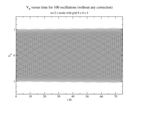
Figure 1: Time evolution of the $\vartheta$ component of velocity on the equator for the linear $m=2$ r-mode in a incompressible and rigidly rotating fluid. The run is supposed to last exactly 100 times the period of this mode which is $\frac{3}{4\Omega}$. The beating phenomenon which can be seen is due to the resolution of the graphical tool. See the power spectrum in figure (3).

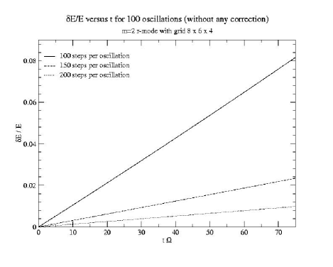
Figure 2: Time evolution of the relative error in the energy before any improvement of the conservation of energy. The different straight lines correspond to runs with the same duration (100 periods of the $m=2$ linear r-mode), same spatial grid ($8\times 6\times 4$ points) but different time steps. We see the linear variation of these errors with time. It shows that exception done of round-off errors (which are so small that they do not appear here), the main error is deterministic and then well controlled.

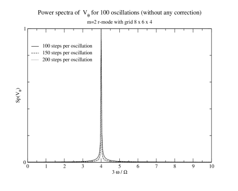
Figure 3: Power spectra of component drawn in figure (1) and of the same component calculated with 150 or 200 steps per oscillation. See also figure (2).

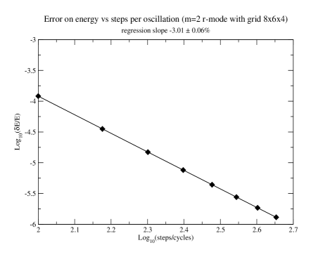
Figure 4: On this picture clearly appears the fact the error exactly comes from the adopted numerical scheme with an error that vanishes as the third power of the time step. The relative error and the number of steps per oscillation are both in logarithmic scales and the regression slope is then $-3.01\,\pm\,0.06\%$.

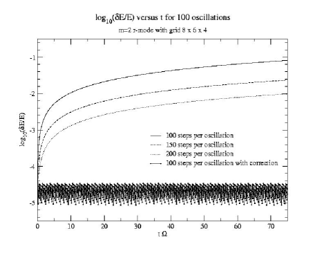
Figure 5: Here are pictured the same curves as in fig.(2), but in logarithmic scales. We added the curve corresponding to a run with 100 steps per period of the $m=2$ linear r-mode with the correction of the conservation of energy described toward Eq.(19).

IV.2 Modes driven to instability in the rigidly rotating case

After trying to improve the conservation of energy for the free case, we did tests with a RR force included. For instance, we switched on the RR force in order to drive toward instability the linear $m=2$ r-mode. As it has already been implied in Section II.3, we did it by using a modified version of the formulae (4) (see this section). For these calculations, we compared numerical results with analytical calculations, both reached with the same approximation. We took for the background star a homogeneous NS with $M=1.4M_{\odot}$, $R=10$ km and $\Omega\sim\left(2\pi\right)500Hz$. In fig.(6) appear two time evolutions of the ratio between the energy and the inertial energy for 100 oscillations of the mode. The first calculation was done without the enhanced conservation of energy and the second with this improvement. The analytical calculation gives for the ratio a final value of the order of $1.0575$ whose difference with the improved numerical value, $1.0582$, is less than $10^{-3}$.

The next step was to switch on the RR force, but without the linear r-mode for initial data, even if we still assumed that the fluid was divergence free. Instead, we chose for the initial velocity a random Gaussian noise with a first moment equal to $0$ and a second moment equal to $1$. It should be noticed that in this case and others where the initial energy is not only distributed within quite low frequency modes, the above method to improve the conservation of energy is no longer appropriate and we shall not use it. Moreover, even if this method does not change the angular momentum when applied to the $m=2$ part of the velocity, it can if one naively applied it to the $m=0$ part. But, as we already mentioned, here we only deal with the linear code and mainly with $m=2$ velocities. And in this case, we exactly control the error done, without changing the angular momentum. We drew in figures (7) and (8) the time evolutions of the $r$ and $\vartheta$ components of the velocity and their power spectra. In fig.(9) is illustrated the time evolution of one of the two independent components of the $S_{ij}$ tensor, with the associated power spectrum. These calculations were done with a lattice of the shape $(12\times 8\times 4)$, with $200$ steps per oscillation and lasted $200$ times the period of the $m=2$ r-mode. The included RR force corresponds to what should exist in a NS with $M=1.4M_{\odot}$, $R=10$ km and $\Omega\simeq(2\pi)\,1050Hz$. Thus, this calculation is not really physical (due to the use of the slow rotation approximation) but just aims at giving a qualitative idea of what should happen with physical values. As expected, there is an axial mode (no radial velocity) driven to instability with exactly the frequency ($w=\frac{4}{3}\Omega$) and coefficients ($l=2$) of the r-mode. Moreover, a single look at the figure (9) shows that even when the velocity is mainly noisy, the tensor that plays the key-role in the instability is quite smooth. In this figure, we also drew a zoom corresponding to $t\Omega<50$ and the associated power spectrum. It shows two frequencies in this component of the tensor. One of them is the unstable r-mode with $3w/\Omega=4$ and the other (with $3w/\Omega\sim 2.70$) disappears with a longer run, as the scale is adapted to the growing mode. Yet, even in the spectrum of the full evolution, a trace of it can still be seen. We achieved exactly the same features with others noisy initial conditions, for instance a Dirac kick into the NS. We also did the same calculations with other spatial lattices (up to $64\times 48\times 4$), and this result did not change at all.

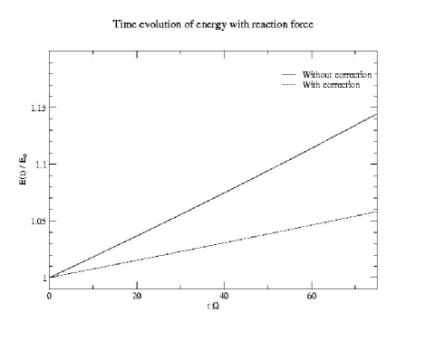
Figure 6: Time evolution of the ratio between energy and initial energy in an inviscid and incompressible rigidly rotating fluid with a RR force corresponding to what should exist in a NS with $M=1.4M_{\odot}$, $R=10$ km and $\Omega\simeq(2\pi)\,500Hz$. The first curve corresponds to the basic code and the second one to the code with improved conservation of energy. The expected final value is about $1.057$. The difference between this analytical calculation and the corrected numerical result is less than $10^{-3}$.

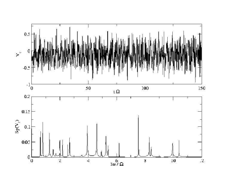
Figure 7: Time evolution of the radial component of velocity in an inviscid and incompressible rigidly rotating fluid with Gaussian noise for initial data and associated power spectrum. A huge RR force acts, but as expected, no polar counter part of the mode grows.

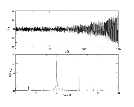
Figure 8: Time evolution of the $\vartheta$ component of velocity on the equator in an inviscid and incompressible rigidly rotating fluid and associated power spectrum with same initial data in fig.(7). Here, the $l=m=2$ linear r-mode is clearly driven to instability by the RR force. As expected, its frequency is $w=\frac{4}{3}\Omega$. Others peaks are just marks of the initial noise.

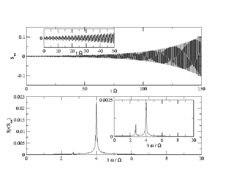
Figure 9: Time evolution of one of the two independent components of the $S_{ij}[t]$ tensor that appears in the RR force. This calculation was done during the same run as the results in fig.(7) and (8). We can also see the almost monochromatic associated spectrum. Nevertheless, there is another frequency in this tensor that is not driven to instability. It can be seen more easily in the zoom of the time evolution or in the corresponding power spectrum.

IV.3 Test of the anelastic approximation

The last calculations we did in a rigid and Newtonian background were to test the effect of the anelastic approximation. The idea was to compare the previous results obtained with the divergence free approximation and a rigid crust BC with results coming from the same initial conditions but with the anelastic approximation and the free surface BC. For the rest of this section, the background star is a polytrope with $\gamma=2$.

First, we took for initial data the linear $l=m=2$ r-mode and let it freely evolve. Here again, the BC do not play any role. The spatial lattice was $(8\times 6\times 4)$ with 100 time steps per period of the mode. The time evolution of $V_{\vartheta}$ at the equator [same as in fig.(1)] did not show any difference with the divergence free case, even for the power spectrum. But this is quite obvious to understand when looking at both the Eq.(17) and the EE. Indeed, we see that the linear r-mode, which is divergence free and has no radial component, is still an eigenvector of this system of equations. Then taking it for initial data in the divergence free case or in the anelastic approximation should give exactly the same evolution. We verified [see fig.(10)] that the radial component of the velocity does not grow and neither does its divergence. This calculation took 344.6 of CPU time without any optimization and with a very basic solving of the anelastic equation.

The next step was the driving toward instability of a mode with noise for initial data. We took exactly the same conditions (duration, lattice, initial data) as in the divergence free case, exception done of the boundary conditions. For these calculations and all that follows with the anelastic approximation, we will use the free surface condition that is automatically satisfied (see the appendix for more details). The figures (11), (12) and (13) that show respectively the time evolutions of $V_{r}$, of $V_{\vartheta}$ and of a component of $S_{ij}$ give a kind of summary of the results:

• the radial velocity still remains noisy and does not grow;

• the $\vartheta$ component grows in the same way as in the divergence free case. There is a difference between the final amplitudes that comes from the fact that the coupling to the RR force depends on an integral on the whole star of a function that is proportional to the density (and then depends on the EOS). Note that the power spectra have the same secondary peaks as in the divergence free case.

• the spectrum of the $S_{ij}$ tensor shows that there is only one unstable mode which has again the frequency of the linear r-mode.

The conclusion is then that the anelastic approximation gives results very close of those obtained in the divergence free case. This is due to the fact that, in spite of the presence of all modes in the initial conditions, the only growing mode is the r-mode that has no radial velocity and is divergence free.

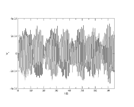
Figure 10: Time evolution of the radial component of the velocity in the equatorial plane in $\xi=0.5$ with the linear $m=2$ r-mode for initial data. The background star is a rigidly rotating $\gamma=2$ polytrope and the calculation is done with the anelastic approximation and without any RR force. The run lasts 100 times the period of the r-mode. There should be no radial velocity (cf. text) and we see it comes only from round-off errors (double precision calculation with initial values of the order of the unity).

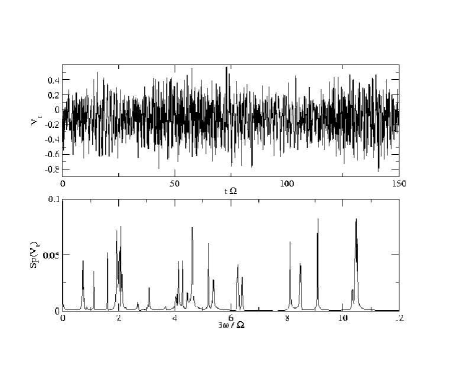
Figure 11: Time evolution of the radial component of velocity with Gaussian noise for initial data and its power spectrum. The background is a polytrope with $\gamma=2$ and the anelastic approximation is used. As in fig.(7) a huge RR force acts, but as the star is rigidly rotating no polar counter part of the mode grows.

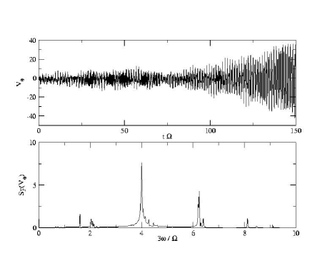
Figure 12: Time evolution of the $\vartheta$ component of velocity and associated power spectrum for the same calculation as in fig. (11). The only difference with the divergence free case [cf. fig.(8)] is the final amplitude. Yet, this is not due to the anelastic approximation but to the effect of the EOS on the coupling coefficient of the RR force.

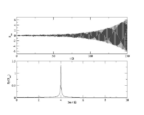
Figure 13: Time evolution of one of the two independent components of the $S_{ij}[t]$ corresponding to the same run as the results in fig.(11) and (12). Here can really be seen the fact that there is only one unstable mode with the frequency of the linear r-mode and that the anelastic approximation does not change this feature.

V Differential rotation

As we already mentioned it in the introduction, Kojima first noticed (see Kojima 1998 koj98 ) that relativistic r-modes may be quite different from what they are in a Newtonian background due to frame dragging. Yet, since the main reason for this difference is the modification of the NSE and the possible appearance of what is called a continuous spectrum (see Ruoff et al. 2001 ruoff01 , ruoff01b and Beyer et al. 1999 beyer99 ), the same may append even in the Newtonian case if the star is not rigidly but differentially rotating. And there are several reasons why a NS may not be in rigid rotation. First, the birth conditions of the NS themselves. Secondly, the non-linear coupling of modes. Then, a possible drift induced by the existence of a magnetic field. As we are here only dealing with linear hydrodynamics and tests of the code, we will not give more details about those processes (and send the reader to the following articles for more details: Spruit 1999 spr99 , Rezzolla et al. 2000 rezls00 , 2001 rezlms01 and rezlms01b , and Schenk et al. 2002 sch02 ). What we have done is just to take as given that the background star is differentially rotating with quite an arbitrary law and to look at the influence of this law on the existence of the modes. Nevertheless, instead of asking the question “Is there any r-mode left in a differentially rotating NS?” that is not well defined, we decided to try to answer to two different and more precise questions:

• is there anything growing when a RR force is applied on noise in a differentially rotating background?

• what does happen to the linear r-modes if they are chosen to be the initial data in such kind of background?

Some lights on these questions are in the following subsections, but we shall begin with some words about the modifications implied on the equations by differential rotation.

V.1 Modifications

Assuming differential rotation of the background star involves slight modifications of what we said in the Section II. First, terms coming from the spatial derivatives of the non constant $\vec{\Omega}[\xi,\vartheta,\varphi]$ must be added in the NSE. Secondly, we shall now specify what exactly means $\Omega$ in the definition of dimensionless variables [cf. Eq.(6)].

Concerning $\Omega$, we chose to take for a time unit the inverse of its value at the equator. This is uniquely determinate due to the fact we have always assumed that the rotation law is of the form $\Omega[r,\vartheta,\varphi]=\Omega[r\sin[\vartheta]]$ or of the form $\Omega[r,\vartheta,\varphi]=\Omega[r]$. The first case corresponds to what must be this law for the background to be stable with respect to the Newtonian EE, and the second case is in a way inspired by GR even if it is not a solution of the full Newtonian EE. For more details see Section VI.

In the dimensionless NSE, the modifications induced by differential rotation are quite simple. First, $\partial_{\varphi}$ is replaced with $\tilde{\Omega}[r,\vartheta]\partial_{\varphi}$ where $\tilde{\Omega}[r,\vartheta]$ is the dimensionless profile of rotation. Then, we have to add new terms coming from $\vec{\rm e}_{\varphi}\,r\sin[\vartheta]\,\vec{V}\cdot\vec{\nabla}\left(\tilde{\Omega}[r,\vartheta]\right)$ that are in the spherical orthonormal basis

$$\left|\begin{array}[]{ll}&0\\ &0\\ V_{r}r\sin[\vartheta]\partial_{r}{\tilde{\Omega}}&+\,\,V_{\vartheta}\sin[\vartheta]\partial_{\vartheta}{\tilde{\Omega}}.\\ \end{array}\right.$$ (20)

V.2 Noise with huge RR force

Once again, our goal was to stay as close as possible of the basic and well understood situation to minimize the number of unknowns. Thus, we took noisy initial data, put it in a differentially rotating background, switched on the RR force and looked to what was to happen. By this way, the question was not to look for the existence of r-modes, but simply to look for the existence of modes driven to instability by the RR force in a non rigidly rotating background.

The only difference with the basic study done in the case of rigid rotation was that we had to choose a law for $\Omega$. The first choice was very simple and corresponded to a background stable with respect to the Newtonian EE. It was of the form

$$\tilde{\Omega}[r,\vartheta]={\cal W}\left(1+\beta_{n}\,r^{2}{\sin[\vartheta]}^{2}\right)$$ (21)

where $\beta_{n}$ was a constant depending on the run and ${\cal W}$ calculated to have $\tilde{\Omega}\left[1,\frac{\pi}{2}\right]=1$. As explained above, we also tried a law inspired by GR:

$$\tilde{\Omega}[r,\vartheta]={\cal W}\left(1+\beta_{gr}\,r^{2}\right)$$ (22)

or laws coming from the already quoted article by Karino et al. karino01 :

$$\tilde{\Omega}[r,\vartheta]=\frac{{\cal W}\,{\beta_{L}}^{2}}{r^{2}{\sin[\vartheta]}^{2}+{\beta_{L}}^{2}}$$ (23)

or

$$\tilde{\Omega}[r,\vartheta]=\frac{{\cal W}\,{\beta_{v}}}{{\left(r^{2}{\sin[\vartheta]}^{2}+{\beta_{v}}^{2}\right)}^{1/2}}.$$ (24)

Since in all these laws, none of the free parameters $\beta$ corresponds to a physical variable, we will not give quantitative results. It will be done in the relativistic study (and then in another article) where there is a parameter that physically quantifies the way the equations are far from the Newtonian EE: the compactness of the star. Here we will only discuss in a qualitative way the results obtained in all the previous cases and give a very representative example: what happens in a $\gamma=2$ polytrope with anelastic approximation (free surface) and the rotation law given by the Eq.(21) with $\beta_{n}=0.4$. Exception done of these choices, the calculation was done with exactly the same conditions as in the last study with noisy initial data in the previous section.

The main difference with the case of rigid rotation is that the mode that grows is no longer purely axial. Indeed, we can see on fig.(14) that the radial velocity is now also driven to instability. Moreover, comparing power spectra in this figure and in fig.(15) and (16) shows that this is really a single mode with frequency very close of the frequency of the r-mode. By a single mode, we mean that this is exactly the same frequency for several physical quantities and several positions in the star. This is not a sufficient condition to talk about “discrete spectrum”, but it is a necessary condition. This unavoidable existence of a polar part of the velocity in a differentially rotating Newtonian star with barotropic EOS should be compared with the results achieved by Lockitch et al. lockandf01 in the relativistic framework. Indeed, in GR, the main reason for the coupling between axial and polar parts of the velocity is the frame dragging that is imitated in a Newtonian framework by differential rotation. Finally, note that the value of the frequency in the Newtonian case is depending on the way we chose to normalize $\Omega$. Then, to summarize all our calculation, we can say that we observed that the polar counter part of the mode appears as soon as there is differential rotation, and whatever the chosen law. Yet, the more the law for $\Omega$ is far from the rigid case, or in more pragmatic way the greater the free parameter is, the more the unstable mode has a polar counter part.

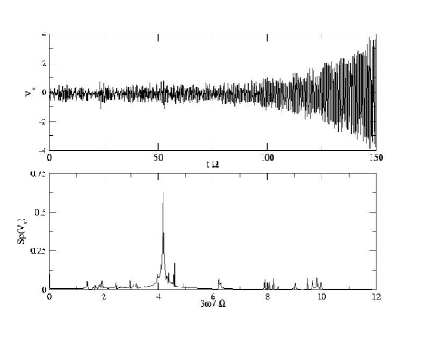
Figure 14: Time evolution of the radial component of velocity in a $\gamma=2$ polytrope with anelastic approximation and Gaussian noise for initial data. A huge RR force acts (something like what should exist in a star with angular velocity equal to $1000$ Hz) and the background star is assumed to be differentially rotating with the law corresponding to $\beta_{n}=0.4$. We see that a polar counter part of the mode now grows.

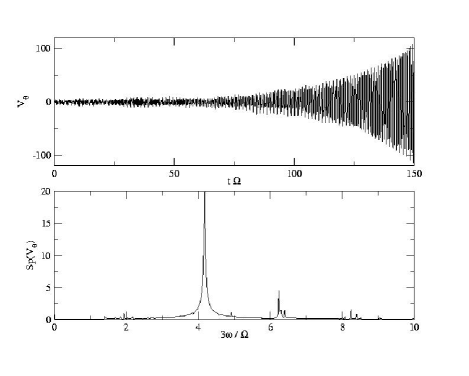
Figure 15: Time evolution of the $\vartheta$ component of velocity in the same calculation as in fig.(14). The associated power spectrum shows that there is one mode driven to instability that is the same as in fig.(14) and has a frequency very close of the expected frequency of the r-mode. See also the fig.(16).

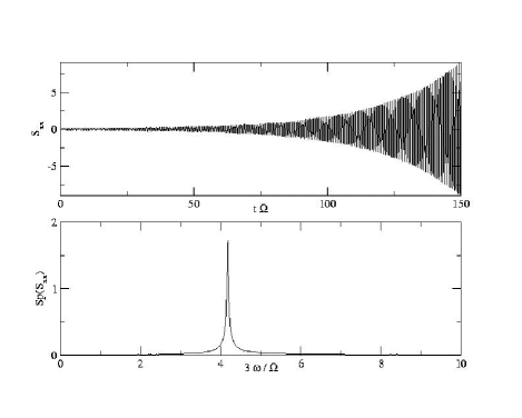
Figure 16: Time evolution of one of the two independent components of the $S_{ij}[t]$ tensor that appears in the RR force. This calculation was done during the same run as the results in fig.(14) and (15). We can see the almost monochromatic associated spectrum with the same frequency as in the previous spectra of the unstable mode.

V.3 Free evolution

The other question we asked was: “What does happen to linear r-modes if they are put into a differentially rotating background?”. The idea in taking such kind of initial data was to have something quite close of an eigenvector, assuming if there is one it should be quite similar to the linear r-mode.

Once again, we did not make quantitative calculations and postponed it to the GR case. As in the case of noisy initial data driven toward instability by a RR force, the free evolution of the linear r-mode showed the growth of a polar part of the velocity. It can be seen on figures (17) and (18) that respectively show the time evolution of the ratio between the polar energy and the total energy and the time evolution of the radial velocity at the point of coordinates $\left(\xi=\frac{1}{2},\vartheta=\frac{\pi}{2},\varphi=0\right)$. This results comes from a calculation done with a spatial lattice of the shape $(64,48,4)$, the anelastic approximation (with a free surface) and a rotation law given by the Eq.(21) with $\beta_{n}=0.4$. For reasons that will be explained later, we included degenerate viscosity (cf. Section III.4) with an Ekman number $E_{s}\,=\,5.\,10^{-5}$ in order to regularize the solution. The evolution was done to last $30$ periods of the linear r-mode with $100$ steps per oscillation. In the figure (17), we see that, after a while, the ratio between the energy in the polar part of the mode and the total energy reaches a kind of stationary state with a coupling between different modes. The existence of this “hybrid final state” was verified during other runs with other physical conditions and is once again to compare with results achieved in GR by Lockitch et al. lockandf01 .

Concerning the existence of modes, looking simultaneously at fig.(18), (19) and (20) shows that apparently one single mode mainly appears in the reaction force (or in the component of the corresponding tensor) even if both axial and polar part of the velocity contain several modes. Yet, the spectrum of the $S_{ij}$ tensor is quite noisy due to the fact that the RR force is not switched on and that the run is short. We verified this feature during other calculations. The conclusion is that for small values of the $\beta$ parameter (these values are depending of the chosen rotation law), the main effect of differential rotation on a “free linear r-mode” is to give it a polar counter part and to widen its spectrum. But for larger values of the parameter, even if the velocity’s spectrum becomes very noisy, the $S_{ij}$ tensor is always less noisy. Yet, here we will not give more details about this points, the linear Newtonian study being not really interesting from the NS point of view.

To end with this section, we will mention a quite amazing feature found in all our calculations and illustrate it with an example coming from the previous free run of a linear r-mode put in the differentially rotating background. We always found that quite fast (in something like $15$ periods of the linear r-mode) the main part of the velocity is most of the time concentrated in a region close of the surface of the star and of the equator. This is illustrated in the figure (21) where we drew the shape of the $\varphi$ component of the velocity versus the radius of the star for several values of the $\vartheta$ angle. Note that we got the same results with different BC and even when we add viscosity to regularize the solution (and this is the case in this calculation) and to be sure this is not a numerical artifact. In fig.(22) appears the shape of $\vartheta$ component for an evolution done with the same grid, viscosity and initial data but with $\beta_{n}=0.8$. With such a huge value of the parameter that governs the rotation law, there is a lot of different modes that appear in the velocity spectrum. But what seems to be the most important result is the very high concentration of the velocity near the surface. This is analogous to the results achieved by Karino et al. in 2001 karino01 . In the conclusion, we will shortly discuss what is, in our point of view, a possible important repercussion of this result.

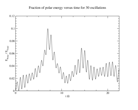
Figure 17: Time evolution of the ratio between energy contained in the polar part of the velocity and the total energy of the mode in the anelastic approximation with a free surface. The background star is assumed to be a $\gamma=2$ polytrope differentially rotating with the law corresponding to $\beta_{n}=0.4$. A viscous term coming from the degenerate viscosity with $E_{s}=5.\,10^{-5}$ is included. At the beginning of the evolution, there is energy coming from the purely axial initial data (the linear r-mode) and going to the polar part. Then this energy oscillates from the polar part of the velocity to the axial part and back with a constant mean value.

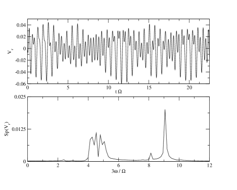
Figure 18: Time evolution of the radial component of velocity with the anelastic approximation and a free surface. This calculation was done during the same run as in fig.(17). The initial data are the linear r-mode that is no longer an eigenvector and radial velocity quickly appears. Several different modes are present.

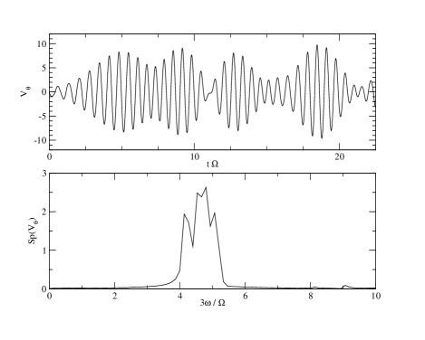
Figure 19: Time evolution of the $\vartheta$ component of velocity in the same calculation as in fig.(18). The curve and the associated power spectrum show that there are several modes, but only one of them appears in the $S_{ij}$ tensor with quite a huge amplitude. Moreover, it has a frequency very close of the frequency of the linear r-mode. See also the fig.(20). Note finally that the same frequency also appears in the spectrum of the radial velocity.

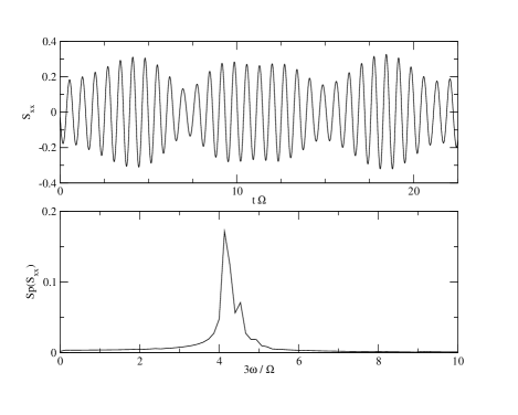
Figure 20: Time evolution of one of the two independent components of the $S_{ij}[t]$ tensor that appears in the RR force. This calculation was done during the same run as the results in fig.(18) and (19). We can see there seems to be one main frequency and a second one of smaller importance. The first one has exactly the same frequency as the unstable mode that appears in the previous figures and calculations where the RR force was on.

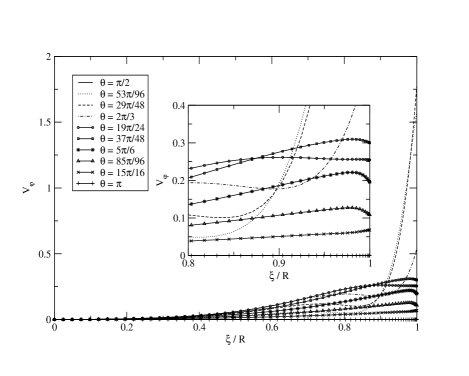
Figure 21: $\varphi$ component of the velocity versus the radius for several values of $\vartheta$. We can see the main part of the velocity is concentrate in a region near the surface and close of the equator. This “snapshot” of the profile was taken at a moment when the derivative versus the radial coordinate of the velocity is quite huge at the surface.

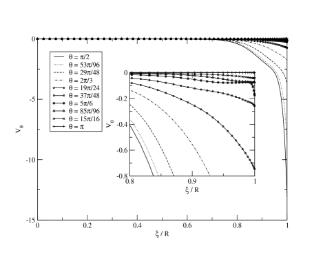
Figure 22: $\vartheta$ component of the velocity versus the radius for several values of $\vartheta$. Here the concentration of the motion is higher than in the previous calculation. $\beta_{n}$ was $0.4$ in fig.(21) and is now $0.8$. Moreover, this calculation lasted three time longer. Nevertheless, note that here we did not choose to draw the profile when the derivative is huge and just drew it at the final instant.

VI Strong Cowling approximation in GR

NS are among the most relativistic macroscopic objects made of usual matter in the Universe. Moreover, the instability of r-mode is due to GR. It is then quite natural to try to study r-modes in the GR framework. The problem is that it is quite difficult to evolve dynamically the full GR and hydrodynamics equations taking into account GW. This is the reason why we decided to use the strong Cowling approximation at the beginning.

Here we will only give some preliminary results obtained in the GR case. A more complete and physical study will be in a following article in preparation. Our goal is just to show that the above conclusions concerning the appearance of a polar part of the velocity and the “concentration of motion” for Newtonian differentially rotating NS still hold in the framework of relativistic rigidly rotating NS.

As we are studying slowly rotating NS, which remain spherical, a very convenient and good approximation is to assume that the $3$-space is conformally flat (see Cook et al. 1996 cook96 ). Furthermore, as we are using the strong Cowling approximation, there is no GW even without this approximation. Then, in unit $c=1$, the infinitesimal space-time interval can be written

$${ds}^{2}=-\left({N[r]}^{2}-{a[r]}^{2}\,r^{2}\,{\sin[\vartheta]}^{2}\,{N^{\varphi}[r]}^{2}\right){dt}^{2}-2{a[r]}^{2}\,r^{2}\,{\sin[\vartheta]}^{2}\,N^{\varphi}[r]dt\,d\varphi+{a[r]}^{2}\,{d\vec{r}}^{2}$$

where, following the $3+1$ formulation, $N[r]$ is the lapse function and $N^{\varphi}[r]$ the third contravariant component on the spherical coordinate basis of the shift vector, ${a[r]}$ is the conformal factor and finally ${d\vec{r}}^{2}$ is the infinitesimal interval in the $3$-space. In this equation, we use the isotropic gauge and the slow rotation limit to assume that all these unknown functions are only depending on $r$ (and this is the reason why, in the Newtonian study, we called “inspired by GR” the law of differential rotation in which the functions are only depending on $r$). In Hartle 1967 hartl67 , the system of coordinates is not the same as the one we use, but it is easy to show that the conclusions are identical since the mapping between the two systems is quite trivial. Furthermore, from the same article we know that ${N^{\varphi}[r]}$ is of the first order in $\Omega$.

To get the equations of motion, the relativistic equivalent of EE, we write the energy tensor of a perfect fluid

$$T^{\mu\nu}=(\rho+p)U^{\mu}U^{\nu}+pg^{\mu\nu}$$ (25)

where $\rho$ is the energy density, $p$ the pressure and $U^{\mu}$ the $4$-velocity of the perfect fluid. Then, we apply the conservation of energy:

$$\nabla_{\mu}T^{\mu\nu}=0.$$ (26)

If we define the generalized enthalpy:

$${\rm{d}}H\widehat{=}\frac{{\rm{d}}P}{\rho+p},$$ (27)

it gives

$$U^{\mu}\,U^{\nu}\,\nabla_{\nu}H\,+\,\nabla^{\mu}H\,+\,U^{\nu}\,\nabla_{\nu}U^{\mu}\,=\,0.$$ (28)

It is well-known that due to thermodynamics, the system of equations obtained by adding the baryonic number conservation $\nabla_{\mu}\left(n\,U^{\mu}\right)$ (where $n$ is the baryonic density) to those four equations is a degenerate system. Then, we chose to work with the baryonic number conservation and the projections on the $3$-space of Eq.(28).

Following the Newtonian case, we just have to add Eulerian perturbations to the rigid rotation and to linearize the equations with respect to both the amplitude of these perturbation and $\Omega$. For the generalized enthalpy, the definition of the perturbation is obvious, but for the full $4$-velocity, we use the well-known results about rigid rotation of relativistic stars and write it as

$$U^{\mu}[t,r,\vartheta,\phi]\,=\frac{1}{N[r]}\left|\begin{array}[]{ll}1+\delta U^{0}[t,r,\vartheta,\phi]&\\ {\left(\frac{N[r]}{a[r]}\right)}^{2}\,\delta U^{r}[t,r,\vartheta,\phi]&\\ {\left(\frac{N[r]}{a[r]}\right)}^{2}\,\frac{\delta U^{\vartheta}[t,r,\vartheta,\phi]}{r}&\\ \Omega+{\left(\frac{N[r]}{a[r]}\right)}^{2}\,\frac{\delta U^{\varphi}[t,r,\vartheta,\phi]}{r\sin[\vartheta]}&\\ \end{array}\right.$$ (29)

Note that in this equation, $\delta U^{0}$ is not a dynamical variable but is determined according to the constraint that $U^{\mu}$ is a $4$-velocity ($U^{\mu}U_{\mu}=-1$). Furthermore, $\delta U^{r},\delta U^{\vartheta}$ and $\delta U^{\varphi}$ are not contravariant components of a $4$-vector but convenient variables that are the components of a $3$-vector on the orthonormal basis associated with the spherical system of coordinates for the flat $3$-space. It enables us to write the motion equations in a way very similar to the Newtonian EE. Indeed, writing the $3$-velocity on the orthonormal basis associated with the spherical coordinates as

$$\vec{V}\widehat{=}\,\left|\begin{array}[]{l}\delta U^{r}\\ \delta U^{\vartheta}\\ \delta U^{\varphi}\\ \end{array}\right.$$ (30)

and defining on the same basis

$$\overrightarrow{\varpi}[t,r,\vartheta,\phi]\widehat{=}\left\{\begin{array}[]{ll}\left(\Omega\,-\,N^{\varphi}[r]\right)\cos[\vartheta]&\\ -\,\sin[\vartheta]\,\left(\Omega\,-\,N^{\varphi}[r]\,+\,A[r]\,\right)&\\ 0&\\ \end{array}\right.$$ (31)

with $A[r]\widehat{=}\,\left(\Omega\,-\,N^{\varphi}[r]\right)\left(\frac{{\rm{d}\ln}[\frac{a[r]}{N[r]}]}{{\rm{d}\ln}[r]}\right)\,-\,\frac{r\,N^{\varphi^{\prime}}[r]}{2}$ where ^′ is the derivative versus the radial coordinate, we have

$$\left(\partial_{t}+\Omega\,\partial_{\varphi}\right)\,\vec{V}+\,2\,\vec{\varpi}\wedge\vec{V}+\vec{\nabla}h=0.$$ (32)

This equation is very close of the Newtonian EE, the main difference being that the $3$-vector that appears instead of $\vec{\Omega}$ is now depending on the coordinates (as in the case of differential rotation) but no longer parallel to the rotation axis.

Concerning the baryonic number conservation, writing it in a Newtonian like way, we have in the slow rotation limit

$$\left(\partial_{t}+\Omega\,\partial_{\varphi}\right)\,\tilde{n}+{\left(\frac{N[r]}{a[r]}\right)}^{2}\rm{div}\left(\tilde{n}\,\vec{V}\right)=0$$ (33)

where $\tilde{n}$ is defined as $\tilde{n}\widehat{=}n\,N^{2}\,a$, $n$ being the baryonic number density. The natural generalization of the anelastic approximation is then

$$\rm{div}\left(\tilde{n}\,\vec{V}\right)=0.$$ (34)

As we are using the strong Cowling approximation, the background star appears in the equations of motion only as “external” (from the point of view of the mode) data. For any relativistic calculation, what we do is to calculate the background configuration using the already existing code illustrated in Bonazzola et al. 1993 bona93 and then to use the resulting lapse, shift, conformal factor and their derivatives with respect to the radial coordinate in our equations.

Here we will only give one single example, showing we have in this relativistic case with the strong Cowling approximation results similar to those obtained in the case of the Newtonian differential rotation. We took a $\gamma=2$ polytrope with $1.74$ solar masses and a radius equal to $12.37$ km. The star was very slowly rotating (the ratio between its kinetic energy and its mass energy was about $10^{-16}$) and we took for a time unit the inverse of the angular velocity. The anelastic approximation with the free surface BC was used and to regularize the solution, we added a degenerate viscosity with $E_{s}=5.\,10^{-5}$ once the final equations were written in a Newtonian way. We insist on the fact that this viscous term does not come from relativistic calculations and just aims at regularizing the solution. In figures (23), (24), (25), (26) and (27) are plotted exactly the same quantities as in the Section V. The conclusions for this preliminary relativistic calculation are the same as in the Newtonian case: a polar counter part of the velocity appears from the beginning of the evolution and most of the time, the velocity is concentrate near the equator and the surface.

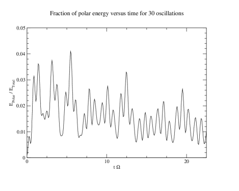
Figure 23: Time evolution of the ratio between energy contained in the polar part of the velocity and the total energy of the mode with the strong Cowling and anelastic approximations and the free surface BC. The background star is a $\gamma=2$ relativistic rigidly rotating polytrope with $1.74$ solar masses and a radius equal to $12.37$ km. The ratio between its kinetic energy and its mass energy was $10^{-16}$. We see that in spite the fact the initial data are the linear Newtonian r-mode that is purely axial, as soon as the calculation begins, a polar counter part of the mode appears as implied by Lockitch et al. lockandf01 .

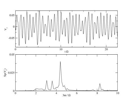
Figure 24: Time evolution of the radial component of velocity at the point $(\frac{1}{2},\frac{\vartheta}{2},0)$ for the same calculation as in fig.(23). The initial data are the linear r-mode that is no longer an eigenvector and radial velocity appears very fast. The power spectrum of the time evolution shows several peaks, but one of them has the same frequency as the modes of fig.(25) and (26) and is the relativistic analog of the r-mode. But it is no longer purely axial.

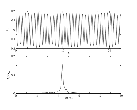
Figure 25: Time evolution of the $\vartheta$ component of velocity in the same calculation as in fig.(24). The curve and the associated power spectrum show that there is one mode that also appears in the polar part with a frequency very close of the frequency of the linear r-mode. See also the fig.(26).

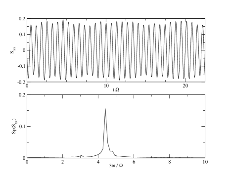
Figure 26: Time evolution of one of the two independent components of the $S_{ij}[t]$ tensor that appears in the RR force. This calculation was done during the same run as the results in fig.(24) and (25). We can see the almost monochromatic associated spectrum with exactly the same frequency as the mode that appears in the previous figures.

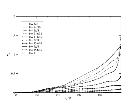
Figure 27: $\vartheta$ component of the velocity versus the radius for several values of $\vartheta$. We can see the kind of concentration of the motion near the surface and the equatorial plane. This calculation was done with the strong Cowling and anelastic approximations and the free surface BC. The background star is a $\gamma=2$ relativistic rigidly rotating polytrope with $1.74$ solar masses and a radius equal to $12.37$ km. The initial data are the Newtonian linear $l=m=2$ r-mode. This figure corresponds to the velocity after a time equal to $15$ oscillations of the linear $l=m=2$ r-mode.

VII Conclusion

This article deals with a new hydrodynamical code based on spectral methods in spherical coordinates. This first version of the code was written to study inertial modes in slowly rotating NS, but it can easily be modified to include fast rotation. As it was explained in the introduction, the slow rotation limit is a very good approximation for a first step. The present version of the code can be used to study both the Newtonian case and the relativistic case with the so-called strong Cowling approximation. Here, we have given the main algorithms it uses and shown some tests of the linear version. The way we overcame the numerical instability is also explained.

Furthermore, in order to work with very different time scales, we have introduced an approximation to deal with mass (or baryonic number) conservation that proved itself quite robust and useful to study inertial modes: the anelastic approximation. Even if this approximation is not a necessary one and can be abandoned in further studies, it is very useful to have an idea of the main properties of the inertial modes in slowly rotating stars. The results presented in this article were obtained in the linear case using very basic models of NS, such as the divergence free case with a rigid crust ($V_{r}\mid_{r=1}=0$) or a $\gamma=2$ polytrope with anelastic approximation and free surface. Deeper studies in the GR framework with more quantitative results on the effects of EOS, of stratification of the star and of BC will follow. Despite the naive aspect of our studies, some common features appeared. Indeed, whatever the approximation (divergence free or anelastic) with different BC (rigid crust for the divergence free case and free surface for the anelastic approximation), we saw the appearance of a polar part in the mode, as soon as the background is Newtonian and differentially rotating, or relativistic and rigidly rotating (in the latter case, this phenomenon is due to the frame dragging). Whether in the case of noisy initial data with a radiation reaction force acting on them, or in the case of the free evolution of an initial linear r-mode, from the very beginning the energy of the polar part is at least one per cent of the energy of the axial part. This result is compatible with the analytical work by Lockitch et al. lockandf01 who proved, in the relativistic framework, the existence of a non-vanishing polar part of the velocity in a sequence of NS with a barotropic equation of state and decreasing rotation rate. Furthermore, another interesting result that we obtained is the “concentration of the motion” near the surface that quickly appears: after less than $15$ periods of the linear r-mode in the calculations done up to now. Adding viscosity has shown that this is a robust and physical feature. Moreover, it seems to neither depend on the physical conditions or on the BC. This phenomenon is very similar to the results found by Karino et al. in 2001 karino01 with a eigenvectors calculation. But, if this is really a singularity of the derivative of the velocity near the surface, as it seems to be in our time evolutions, it would mean that a mode calculation with finite difference schemes can only give quantitative results completely depending on the number of points. Indeed, with this scheme, there is an intrinsic numerical viscosity that depends on the resolution. Moreover, if this phenomenon is verified in following studies in GR, the stratification of the NS or the physics of the crust could be very important to know if inertial modes are relevant for GW emission.

Appendix A Spirit of the pseudo-spectral methods

Our group developed algorithms and routines library (see Bonazzola et al. 1990, 1999 bonam90 ,bonagm99 ) allowing us to solve partial differential equations (PDE) in different geometries, mainly in domains diffeomorphic to a sphere. First, with an example of scalar PDE, we will look at the singularities contained in operators expressed in spherical like coordinates [see for instance the different components of the NSE: Eq.(II.2)] and at our choice of spectral basis. Then, we shall discuss the further difficulties that arise in vectorial PDE and explain the way we overcome them.

A.1 The scalar heat equation

Consider the heat equation:

$$\frac{\partial F}{\partial t}=\alpha\Delta F+S$$ (35)

where $\Delta F=\frac{\partial^{2}F}{\partial r^{2}}+\frac{2}{r}\frac{\partial F}{\partial r}+\frac{1}{r^{2}}(\frac{\partial^{2}F}{\partial\vartheta^{2}}+\frac{\cos\vartheta}{\sin\vartheta}\,\frac{\partial F}{\partial\vartheta}+\frac{1}{\sin\vartheta^{2}}\frac{\partial^{2}F}{\partial\varphi^{2}})$ is the Laplacian in spherical coordinates, $\alpha$ the heat conductivity supposed to be constant, and $S$ a source term (that may include non-linear terms if they exist). The idea of spectral methods is to look for the solution of the Eq.(35) on the form

$$F[r,\vartheta,\varphi,t]=\sum_{n,l,m=0}^{\infty}F_{nlm}[t]\,H^{l}_{n}[r]\,K^{m}_{l}[\vartheta]\,L_{m}[\varphi]$$ (36)

with ($0\leq r\leq 1;0\leq\vartheta\leq\pi;0\leq\varphi\leq 2\pi$) and where $H^{l}_{n}[r],K^{m}_{l}[\vartheta],L_{m}[\varphi]$ are a well chosen complete set of functions. The problem is then to find the time evolution of the coefficients $F_{nlm}[t]$.

In a spherical geometry, it is quite natural to choose $L_{m}[\varphi]=\exp^{im\varphi}$ and $K^{m}_{l}[\vartheta]=P^{m}_{l}[\vartheta]$, where $P^{m}_{l}[\vartheta]$ are the Legendre functions. With these choices, the Eq.(35) can be written

$$\frac{\partial F_{lm}[r,t]}{\partial t}-\alpha\left(\frac{\partial^{2}F_{lm}[r,t]}{\partial r^{2}}+\frac{2}{r}\frac{\partial F_{lm}[r,t]}{\partial r}-\frac{l(l+1)}{r^{2}}F_{lm}[r,t]\right)=S_{lm}[r,t]$$ (37)

where $S_{lm}[r,t]$ are the Fourier-Legendre coefficients of the function $S$ at the radius $r$ and the instant $t$.

In order to handle the singularity at $r=0$, we shall consider separately the cases $l=0$ , $l=1$ and $l>1$:

• For $l=0$, we use the fact that a $C^{1}$ function symmetric with respect to the inversion $r\rightarrow-r$ has its first derivative that vanishes at least as $r$ at $r=0$. Therefore, for such a function, the term $\frac{\partial^{2}F}{\partial r^{2}}+\frac{2}{r}\frac{\partial F}{\partial r}$ is regular. Even Chebyshev polynomials $T_{2n}[r]$ have this property, and the choice $H^{0}_{n}[r]=T_{2n}[r]$ ($n\geq 0$) then satisfies the regularity conditions.

• For $l=1$, it is almost the same, but the final choice is $H^{1}_{n}[r]=T_{2n+1}[r]$.

• The case $l>1$ is more delicate to handle. Indeed, it can be shown (See Bonazzola et al. 1990 bonam90 ) that for $F[r,\vartheta,\varphi,t]$ to be a $C^{\infty}$ function, the coefficients $F_{lm}$ must vanish as $r^{l}$ at $r=0$. It means that the $F_{lm}[r,t]$ are symmetric with respect to the inversion $r\rightarrow-r$ if $l$ is even, and anti-symmetric in the opposite case. We shall then distinguish the two cases $l$ even and $l$ odd.
  

  Case $l>1$ even
  The functions $H^{l}_{n}[r]=T_{2n}[r]-T_{2n+2}[r]$ are even and vanish as $r^{2}$ at the origin. Therefore the quantity $(\frac{\rm{d}^{2}}{\rm{d}r^{2}}+\frac{2}{r}\frac{\rm{d}}{\rm{d}r}-\frac{l(l+1)}{r^{2}})H^{l}_{n}[r]$ is regular at the origin and is retained.
  

  Case $l>1$ odd
  The functions $H^{l}_{n}[r]=(2n+1)T_{2n+1}[r]+(2n-1)T_{2n+3}[r]$ are anti-symmetric with respect to the inversion $r\rightarrow-r$ and vanish as $r^{3}$ at $r=0$. Therefore the quantity $(\frac{{\rm{d}}^{2}}{{\rm{d}}r^{2}}+\frac{2}{r}\frac{{\rm{d}}}{{\rm{d}}r}-\frac{l(l+1)}{r^{2}})H^{l}_{n}[r]$ is also regular and completes our basis.

Note that by this way, we expand the solution with a set of functions that satisfy minimal conditions of regularity, excepted for $l=0$ and $l=1$. It means that they vanish as $r^{2}$ or $r^{3}$, in order to make regular any term in the equation, instead of vanishing as $r^{l}$ as they should to form a $C^{\infty}$ function. Until now, in all the problems that our group treated, these minimal regularity conditions were sufficient (see Bonazzola et al. 1999 bonagm99 for more details). But we shall see later that they make the Euler equations unstable.

To end with the scalar case, we shall show how the Eq.(37) can be written when the time discretization is performed and a $2^{nd}$ order implicit scheme used:

$$F_{nlm}^{j+1}-\alpha\frac{\Delta t}{2}\sum_{p=0}^{\infty}A^{l}_{pn}F_{plm}^{j+1}=F_{nlm}^{j}+{\Delta t}\left(\alpha\frac{1}{2}\sum_{p=0}^{\infty}A^{l}_{pn}F_{plm}^{j}+S_{nlm}^{j+1/2}\right).$$ (38)

Here $A^{l}_{jn}=\langle H^{l}_{j}\,O^{l}\,H^{l}_{n}\rangle$ is the matrix of the operator $O^{l}=\frac{{\rm{d}}^{2}}{{\rm{d}}r^{2}}+\frac{2}{r}\frac{{\rm{d}}}{{\rm{d}}r}-\frac{l(l+1)}{r^{2}}$. The index $j+1/2$ means a quantity $S$ computed at the time $t^{j}+\Delta t/2$, obtained by extrapolating this quantity using its (known) values at time $t^{j-1}$ and $t^{j}$: $S^{j+1/2}=\left(3S^{j}-S^{j-1}\right)/2$. The left hand side operator can be easily reduced to a pentadiagonal one, and then inverted with a number of arithmetic operations that is proportional to the maximum value $N_{max}$ of $N$.

In the case of a space dependent heat conductivity $\alpha[r,\vartheta,\varphi]$, we can use a semi-implicit method (see Gottlieb et al. 1977gott77 ). It consists in solving the equation

$$F_{nlm}^{j+1}-(a+br^{2})\frac{\Delta t}{2}\sum_{p=0}^{\infty}A^{l}_{pn}F_{plm}^{j+1}=$$ (39)

$$F_{nlm}^{j}+\frac{\Delta t}{2}(a+br^{2})\sum_{p=0}^{\infty}A^{l}_{pn}F_{plm}^{j}+{\Delta t}\left(S_{nlm}^{j+1/2}+\left(\alpha-a-br^{2}\right){\left(\sum_{p=0}^{\infty}A^{l}_{pn}F_{plm}\right)}^{j+1/2}\right)$$

where $a$ and $b$ are two coefficients that satisfy the condition $a+br^{2}\geq\alpha$ everywhere and that we choose in such a way that $a+br^{2}$ takes the same values as $\alpha$ at the boundaries.

The new matrix in the L.H.S. is again a pentadiagonal matrix. Boundary conditions are imposed by adding a homogeneous solution of the Eq.(38) or of the Eq.(39). The reader can find in the quoted literature more details on the spectral methods, and on how to implement boundary conditions.

To conclude, note that in the present example, we expand the solution in spherical harmonics. But it turns out that in general it is more convenient to use linear combinations of Chebyshev polynomials to treat the expansion in $\vartheta$. The philosophy of the spectral methods then consists in performing simple operations such as computing derivatives, primitives, integrals, multiplications or divisions by $r$, $r^{2}$, $\sin\vartheta$ or $\cos\vartheta$ in the coefficients space, and by making multiplications of functions in the configuration space. If necessary, the passage to a Legendre representation is performed with a matrix multiplication.

A.2 Analysis in vectorial case

A.2.1 Stability of numerical vectorial PDE

We have seen how to handle coordinates singularities appearing in scalar PDE when spherical coordinates are used. But when treating vectorial PDE, as EE or NSE, the singularities are more malicious: a single look at the components of NSE [Eq.(II.2)] should be sufficient to convince the reader. The singular terms cannot be handled only by laying down analytical properties, as it was done in the above scalar equation. Indeed, the dependence existing among the different spherical components must be taken into account in order to make singular terms compensate each others. A simple example will illustrate this crucial point.

Consider the following constant divergence free vector $\vec{V}$ of Cartesian components: $V_{x}=0,\;V_{y}=0,\;V_{z}=1$. Its spherical components are $V_{r}=-\cos\vartheta;V_{\vartheta}=\sin\vartheta;V_{\varphi}=0$. Then, we have ${\rm{div}}\vec{V}=\frac{\partial V_{r}}{\partial r}+\frac{2}{r}V_{r}+\frac{1}{r}(\frac{\partial V_{\vartheta}}{\partial\vartheta}+\frac{\cos\vartheta}{\sin\vartheta}V_{\vartheta})=0$. A small error (for example a round-off error) in the computation of components will obviously forbid an exact compensation between the two singular terms $2V_{r}/r$ and $\frac{1}{r}(\partial_{\vartheta}V_{\vartheta}+\frac{\cos\vartheta}{\sin\vartheta}V_{\vartheta})$. The consequence is the creation of high order coefficients and possible instabilities appearing in the iterative process.

Indeed, we found that the hydro-code for solving linearized EE was unstable. As expected, high frequency terms were exploding after few hundred time-steps (few periods of the r-mode) either in the case of the anelastic approximation or in the case of the incompressible approximation (${\rm{div}}\vec{W}=0$). As explained above, the main reason of this instability was the non exact compensation of the singular terms contained in the different source terms in the Poisson equations (56) and (58) (see below).

To overcome this problem, we define two angular potentials $T_{h}$ and $P_{o}$ in a such a way that

$$W_{\vartheta}=\partial_{\vartheta}\,P_{o}-\frac{1}{\sin\vartheta}\partial_{\varphi}\,T_{h}$$ (40)

$$W_{\varphi}=\frac{1}{\sin\vartheta}\partial_{\varphi}\,P_{o}+\partial_{\vartheta}\,T_{h}.$$

If $r\,P_{o}$ and $T_{h}$ are any arbitrary set of regular functions, we are now sure that the corresponding components $W_{\vartheta}$ and $W_{\varphi}$ will make the divergent terms appearing in the vectorial PDE compensate each other. Moreover, the system of equations (40) can be easily inverted. First, taking the angular divergence of $W_{\vartheta}$ and $W\varphi$: ${\rm{div}}_{\vartheta\varphi}\vec{W}\widehat{=}(\partial_{\vartheta}+\cot\vartheta\,)W_{\vartheta}+\frac{1}{\sin\vartheta}\partial_{\varphi}\,W_{\varphi}$ gives $\Delta_{\vartheta\varphi}P_{o}={\rm{div}}_{\vartheta\varphi}\vec{W}$ where $\Delta_{\vartheta\varphi}\widehat{=}\partial^{2}_{\vartheta}+\cot\vartheta\partial_{\vartheta}+\frac{1}{\sin^{2}\vartheta}\partial^{2}_{\varphi}$. If ${\rm{div}}_{\vartheta\varphi}\vec{W}$ is then expanded in spherical harmonics, we immediately have

$$P_{o,lm}=-\frac{1}{l(l+1)}({\rm{div}}_{\vartheta\varphi}\vec{W})_{lm}.$$ (41)

It is the same to compute $T_{h}$. Taking the angular curl of $\vec{W}$, we obtain

$$\Delta_{\vartheta\varphi}T_{h}=\rm{curl}_{\vartheta\varphi}\vec{W}$$ (42)

where $\rm{curl}_{\vartheta\varphi}\vec{W}\widehat{=}-\frac{1}{\sin\vartheta}(\partial_{\varphi}W_{\vartheta}-\partial_{\vartheta}(\sin\vartheta\,W_{\varphi}))$.

To complete this procedure, we have to guarantee that $W_{r}$ can also compensate the singular terms generated by the components $W_{\vartheta}$ and $W_{\varphi}$. A satisfactory way to proceed is to take as a new variable the quantity ${\rm{div}}\vec{W}$. Indeed, once the quantity $g[r,\vartheta,\varphi]={\rm{div}}\vec{W}$ is known, it turns to be easy to find $W_{r}$. Bearing in mind that ${\rm{div}}\vec{W}=\partial_{r}W_{r}+2\,W_{r}/r+1/r^{2}\,{\rm{div}}_{\vartheta\varphi}\vec{W}$, we have, after an expansion in spherical harmonics

$$W_{r,lm}=\frac{1}{r^{2}}\int_{0}^{r}u\,\left(u\,{g[u,\vartheta,\varphi]}_{lm}+l(l+1)\,P_{o,lm}[u,\vartheta,\varphi]\right){\rm{d}}u.$$ (43)

Thus, at each time step, the strategy consists in calculating the potentials $P_{o}$ and $T_{h}$, and then in calculating back the components $W_{\vartheta}$ and $W_{\varphi}$. The component $W_{r}$ is also computed at each time step by using the Eq.(43).

Finally, note that with this procedure, the potentials $P_{o}$, $T_{h}$ and the component $W_{r}$ have the correct analytical behaviour on the axis $e_{z}$, i.e they vanish as $\sin^{m}\vartheta$. Thus, the instability of the EE hydro-code was drastically reduced, but not completely suppressed. It still kept on growing, but about ten times slower than before. The reason of this residual instability was that, at each time step, the round-off errors did not have the correct analytical properties at $r=0$. Indeed, they did not vanish as $r^{l}$. Consequently high spatial frequency terms were still generated that did not have the good analytical properties and a runaway toward the instability was once again generated. To avoid this phenomenon, we project, at each time step, all the scalar quantities $({\rm{div}}\vec{W})_{lm}[r]$, $P_{o},_{lm}[r]$ and $T_{h},_{lm}[r]$ on a Legendre space $P^{l}_{n}[r]$ in such a way to satisfy the analytical conditions. Note that the necessity of this procedure is due to the fact that in the EE, solved with spectral methods, no dissipative term (numerical or physical) is present. Consequently the numerical instability are not dumped.

A.2.2 Solving the vectorial heat equation

Now, more details concerning the algorithm to solve vectorial PDE with spectral methods. In solving NSE, we need to solve a vectorial heat equation that can be reduced to an equation of the type

$$\frac{\partial\vec{\hat{B}}}{\partial t}+\nabla\wedge(\mu\nabla\wedge\vec{\hat{B}})=\vec{\hat{J}}$$ (44)

where $\vec{\hat{J}}$ is the divergence free term of the source. We remember that it is obtained by the decomposition of the source term $\vec{J}$ in a potential part $\vec{\nabla}\phi$ and a divergence free part $\vec{\hat{J}}$: $\vec{J}=\vec{\hat{J}}+\vec{\nabla}\phi$.

The Eq.(44) can be written in the following form:

$$\frac{\partial\vec{B}}{\partial t}=\mu\,\triangle\vec{B}+(\nabla\wedge\vec{B})\wedge\vec{\nabla}\mu+\vec{\hat{J}}.$$ (45)

From a numerical point of view, the term $\vec{S}=(\nabla\wedge\vec{\hat{B}})\wedge\vec{\nabla}\mu$ is considered as a source and is computed by a second order scheme using its values at the times $t_{j-1}$ and $t_{j-2}$.

Therefore, we have to solve the equation

$$\frac{\partial\vec{B}}{\partial t}=\mu\Delta\vec{B}+\vec{\hat{J}}+\vec{S}$$ (46)

with the condition $\vec{\nabla}\cdot\vec{\hat{B}}=0$.

The technique generally used was already described in Bonazzola et al. 1999 bonagm99 . Nevertheless, we adopted here a slightly different approach which gives more accurate results.

To solve the Eq. (46) it is convenient to introduce the poloidal and toroidal potentials $P_{o}$ and $T_{h}$ as defined in appendix A.2.1. Here we will only consider the case of $\mu=1$, the semi-implicit scheme which must be used in the more general case being straightforward. With a second order scheme, we have in the harmonic representation

$$P^{j+1}_{o,lm}-\frac{1}{2}\Delta t\left(\frac{{\rm{d}}^{2}P^{j+1}_{o,lm}}{{\rm{d}}r^{2}}+\frac{2}{r}\frac{{\rm{d}}P^{j}_{o,lm}}{{\rm{d}}r}-\frac{l(l+1)}{r^{2}}P^{j+1}_{o,lm}-\frac{2}{r^{2}}\hat{B_{r}}_{lm}^{j+1}\right)=$$ (47)

$$P^{j}_{0,lm}+\Delta t\left(\frac{1}{2}\left(\frac{{\rm{d}}^{2}P^{j}_{o,lm}}{{\rm{d}}r^{2}}+\frac{2}{r}\frac{{\rm{d}}P^{j}_{o,lm}}{{\rm{d}}r}-\frac{l(l+1)}{r^{2}}P^{j}_{o,lm}-\frac{2}{r^{2}}\hat{B_{r}}_{lm}^{j}\right)+\Pi^{j+1/2}_{lm}\right)$$

where $\Pi$ is the poloidal component of $\vec{\hat{J}}+\vec{S}$. Note the presence of a singular term $\frac{2}{r^{2}}B^{j+1}_{r}$ in this equation. Bearing in mind that ${\rm{div}}\vec{\hat{B}}=0$ and that $P^{j+1}_{o,lm}$ vanishes as $r^{l-1}$, it is obvious that there should be a compensation between these two terms. Nevertheless, we shall slightly modify the Eq.(47) in order to obtain more easily this compensation:

$$P^{j+1}_{o,lm}-\frac{1}{2}\Delta t\left(\frac{{\rm{d}}^{2}P^{j+1}_{o,lm}}{{\rm{d}}r^{2}}+\frac{2}{r}\frac{{\rm{d}}P^{j}_{o,lm}}{{\rm{d}}r}-\frac{l(l-1)}{r^{2}}P^{j+1}_{o,lm}\right)=$$ (48)

$$P^{j}_{0,lm}+\Delta t\left(\frac{1}{2}\left(\frac{{\rm{d}}^{2}P^{j}_{o,lm}}{{\rm{d}}r^{2}}+\frac{2}{r}\frac{{\rm{d}}P^{j}_{o,lm}}{{\rm{d}}r}-\frac{l(l-1)}{r^{2}}P^{j}_{o,lm}\right)-\frac{1}{r^{2}}\left(\hat{B_{r}}^{j}_{lm}+l\,P_{0,lm}^{j}+\hat{B_{r}}^{j+1}_{lm}+l\,P_{0,lm}^{j+1}\right)+\Pi^{j+1/2}_{lm}\right).$$

Once $P_{o,lm}^{j+1}$ known, $\hat{B}_{r,lm}^{j+1}$ is obtained as explained above [see Eq.(43), with $g=0$].

Finally, the equation for the toroidal part of $\vec{\hat{B}}$ reduces to an ordinary scalar heat equation:

$$T^{j+1}_{h,(l-1)m}+\frac{1}{2}\Delta t\left(\frac{{\rm{d}}^{2}T^{j+1}_{h,(l-1)m}}{{\rm{d}}r^{2}}+\frac{2}{r}\frac{{\rm{d}}T^{j}_{h,(l-1)m}}{{\rm{d}}r}-\frac{l(l-1)}{r^{2}}T^{j+1}_{h,(l-1)m}\right)=$$ (49)

$$T^{j}_{h,(l-1)m}+\Delta t\left(\frac{1}{2}\left(\frac{{\rm{d}}^{2}T^{j}_{h,lm}}{{\rm{d}}r^{2}}+\frac{2}{r}\frac{{\rm{d}}T^{j}_{h,lm}}{{\rm{d}}r}-\frac{l(l-1)}{r^{2}}T^{j}_{h,lm}\right)+\vartheta^{j+1/2}_{(l-1)m}\right)$$

where $\vartheta$ is the toroidal component of $\vec{\hat{J}}+\vec{S}$.

Appendix B Solving Euler or Navier-Stokes equations

In this section, we shall show how to implement the different schemes proposed in the Section III to handle the different time scales appearing in the EE for a slowly rotating star. In all cases, for simplicity, we will only consider the linearized equations. First, we will begin with the case where the exact system of equations is to solve. Then we shall consider the implementation of physical approximations and finally the problem of BC.

B.1 Exact Euler equations

As usual, we start by doing a decomposition of the velocity vector $\vec{W}$ in a divergence free component $\vec{\hat{W}}$ and a potential one:

$$\vec{W}=\vec{\hat{W}}+\vec{\nabla\Psi},\;\;{\rm{div}}\vec{\hat{W}}=0.$$ (50)

In a second order time scheme, the divergence free component of the EE is then written as

$$\vec{\hat{W}}^{j+1}=\vec{\hat{W}}^{j}+\Delta t\,[-2\vec{\Omega}\wedge\vec{W}+\vec{F}]^{j+1/2}_{DF}$$ (51)

while the potential part is

$$\Psi^{j+1}=\Psi^{j}-\Delta t\,[\varphi_{\Omega}+h+\varphi]^{j+1/2}.$$ (52)

In the Eq.(51), the subscript $DF$ means the divergence free component of the external force. In the Eq.(52), the subscript $\Omega$ is for the potential component of the Coriolis force $2\vec{\Omega}\wedge\vec{W}$, $\varphi$ is the potential component of some other exterior force and $h$ is the variation of the enthalpy. Moreover, we also have the baryonic number (or mass) conservation equation:

$$h^{j+1}=h^{j}-\Delta t\left(\left(\hat{W}_{r}+\frac{\partial\Psi}{\partial r}\right)\,\frac{\partial H_{0}}{\partial r}+\Gamma H_{0}\Delta\Psi\right)^{j+1/2}$$ (53)

where $H_{0}$ is the enthalpy of the non perturbed configuration. In this explicit second order scheme, the required typical value of the time step $\Delta t$, which guarantees the numerical stability, is determined by the term $\partial_{r}H_{0}$ that is much larger than the Coriolis term for a slowly rotating NS.

The implicit version of the system of equations (52), (53) is the following:

$$\Psi^{j+1}=\Psi^{j}-\Delta t\,\left(\frac{1}{2}\left(h^{j+1}+h^{j}\right)+[\varphi_{\Omega}+h+\varphi]^{j+1/2}\right)$$ (54)

$$h^{j+1}=h^{j}-\frac{1}{2}\Delta t\left(\left(\partial_{r}\Psi^{j+1}+\partial_{r}\Psi^{j}+\hat{W}_{r}^{j+1}+\hat{W}_{r}^{j}\right)\partial_{r}H_{0}+\Gamma H_{0}\left(\Delta\Psi^{j+1}+\Delta\Psi^{j}\right)\right)$$

where $\hat{W}_{r}^{j+1}$ is obtained from the Eq.(51). Solving the above system of equations reduces to invert, for each value of $l$ and $m$ an enneadiagonal ($2\,N_{r}\times 9$) matrix (9 diagonals) where $N_{r}$ is the number of degrees of freedom in $r$. The generalization to the NSE is quite obvious and we shall not give more details about it.

B.2 Implementation of physical approximations

As it was already explained in the Section III, for solving the EE or NSE, we chose to use approximations in order to better control the results.

B.2.1 The divergence free approximation

The spirit of this approximation consists in replacing the mass conservation equation (53) by the condition

$${\rm{div}}\vec{W}=0$$ (55)

or equivalently $\Psi=0$. The problem is then to find the enthalpy $h$ in a such a way that the condition (55) is satisfied. This can be done easily by solving the Poisson equation

$$\Delta h-{\rm{div}}F^{j+1/2}=0$$ (56)

reached by taking the divergence of the EE. As the gradient of an harmonic function is a divergence free vector, such a function can then be added to a particular solution of the Eq.(56) in order to satisfy the boundary conditions. Once $h$ is obtained, the EE has to be solved with $\vec{\hat{F}}=\vec{F}-\vec{\nabla}h$. If viscous terms are present, NSE case, a vectorial type equation must be solved.

B.2.2 Anelastic approximation

As it was already explained, the anelastic approximation consists in neglecting the term $\partial_{t}h$ in the Eq.(53). Once again, the game consists in finding the enthalpy $h$ in a such a way that the following equation is satisfied:

$$\Gamma H_{0}\,{\rm{div}}\,\vec{W}+W_{r}\partial_{r}H_{0}=0.$$ (57)

To find $h$, it is sufficient to derive with respect to time the Eq.(57), and to replace $\partial_{t}\rm{div}\vec{W}$ by its value reached from the EE. It gives

$$\Gamma\,H_{0}\,\Delta h+\partial_{r}H_{0}\partial_{r}h=\Gamma\,H_{0}\,{\rm{div}}\vec{F}^{j+1/2}+F_{r}^{j+1/2}\partial_{r}H_{0}$$ (58)

where $\vec{F}$ contains all the force terms (Coriolis force included).

The solution of the above equation is achieved with a semi-implicit scheme very similar to the one used to solve the Eq.(35). The problem is then reduced to solve the following Equation (for simplicity, we shall consider only the case of a polytropic EOS):

$$(\gamma-1)(a+br^{2})\Delta h+2br\partial_{r}h=\bar{H_{0}}\Delta h+\partial_{r}\bar{H_{0}}\partial_{r}h+\rm{div}\vec{F}^{j+1/2}+\partial_{r}H_{0}F_{r}^{j+1/2}$$ (59)

where $a$ and $b$ are two constants defined as was done in solving the Eq.(35). The L.H.S. operator can be easily inverted and the Eq.(59) can be solved by iteration (see Gourgoulhon et al. 2001 gougc01 ). The iteration at each time step being quite time consuming, a more convenient strategy (although less accurate) consists in replacing $h$ in the R.H.S. of the Eq.(59) by $h^{j+1/2}$.

B.3 Boundary conditions

It was already explained how to impose BC for divergence free case. For the system of equations (54) or the Eq.(58), it is worth distinguishing two cases: either the enthalpy vanishes or does not vanish at the boundary of the integration domain. Here we will only consider the case of EE. Indeed, for NSE we chose to take a viscosity that vanishes at the surface to avoid the need of further BC.

If $H_{0}\,|_{r=1}>0$, the solution is quite easy : the Eq.(58) or the system of equations (54) admit an homogeneous solution that can be used to satisfy one BC.

If $H_{0}(1)$ vanishes, the system of equations (54) or the Eq (58) are degenerate and therefore no BC can be imposed. But we shall show that, in this case, the correct BC are automatically satisfied.

Indeed, consider first the case of the linearized exact system of equations (54). On the surface of the non perturbed star, we have $\partial_{t}h+\vec{W}\cdot\vec{\nabla}H_{0}$ that is the the correct BC. The surface $H_{0}+h=0$ then defines the profile of the perturbed star. To show that the solution in the anelastic approximation also satisfies the BC, it is more convenient to first examine the non-linear case. Here, $h$ is not infinitesimal, and the Eq.(57) must be replaced with the equation

$$\Gamma(H_{0}+h)\,{\rm{div}}\,\vec{W}+\vec{W}\cdot\vec{\nabla}(H_{0}+h)=0$$ (60)

that is satisfied if $h$ is a solution of the non linearized Eq (58):

$$\Gamma\,(H_{0}+h)\,\Delta h-{\rm{div}}\vec{F}^{j+1/2}+(\vec{\nabla}h-\vec{F}^{j+1/2})\cdot\vec{\nabla}(H_{0}+h))=0.$$ (61)

Once again, the surface of the star is defined by $H_{0}+h=0$. But from the Eq.(60) we have the correct BC: $\vec{W}\cdot\vec{\nabla}(H_{0}+h)\,|_{H_{0}+h=0}=0$. The surface of the star is then an unknown quantity that is determined by the relation $H_{0}+h=0$ in solving the Eq.(61) by iteration. This technique was developed in a different context in the already quoted paper gougc01 .

In the linear case, we have $W_{r}=0$ at $r=1$ [cf. Eq.(57)], and the enthalpy does not vanish on the non-perturbed surface of the star. But once again the free surface of the star can be obtained by looking for the position where the total enthalpy $H_{0}+h=0$ vanishes. This surface coincides within first order quantities with the non perturbed surface $r=1$. Note that if $\gamma>0$ the pressure $P|_{r=1}\propto h^{\gamma+1}|_{r=1}$ vanishes within terms $o(h)$.

References

- (1) S. Karino, S. Yoshida and Y. Eriguchi, Phys. Rev. D 64, 024003 (2001).
- (2) K.H. Lockitch, N. Andersson and J.L. Friedman, Phys. Rev. D 63, 024019 (2001).
- (3) N. Andersson, Astrophys. J. 502, 708 (1998).
- (4) W. Thomson, Phil. Mag. 10, 155 (1880).
- (5) M. Rieutord, Astrophys. J. 550, 443 (2001); Erratum - ibid. 557, 493 (2001).
- (6) S. Chandrasekhar, Phys. Rev. Lett. 24, 611 (1970).
- (7) J.L. Friedman and B.F. Schutz, Astrophys. J. 221, 937 (1978); 222, 281 (1978).
- (8) J.L. Friedman and S.M. Morsink, Astrophys. J. 502, 714 (1998).
- (9) L. Bildsten, Astrophys. J., Lett. 501, L89 (1998).
- (10) N. Andersson and K.D. Kokkotas, Int. J. of Mod. Phys. D 10, 381 (2001).
- (11) J.L. Friedman and K.H. Lockitch, review in Proceedings of the 9th Marcel Grossman Meeting, edited by V. Gurzadyan, R. Jantzen and R. Ruffini, (World Scientific, Singapore, 2002).
- (12) L. Lindblom, J.E. Tohline and M. Vallisneri, Phys. Rev. Lett. 86, 1152 (2001); Phys. Rev. D 65, 084039 (2002).
- (13) P. Arras, E.E. Flanagan, S.M. Morsink, A.K. Schenk, S.A. Teukolsky and I. Wasserman, Submitted to Astrophys. J. , 25 pages. astro-ph/0202345.
- (14) M. Lesieur, Turbulence in fluids (Martinus Nijhoff Publishers, Dordrecht, 1987).
- (15) S.S. Murray, P.O. Slane, F.D. Seward, S.M. Ransom and B.M. Gaensler, Astrophys. J. 568, 226 (2002).
- (16) F. Camilo, I.H. Stairs, D.R. Lorimer, D.C. Backer, S.M. Ransom, B. Klein, R. Wielebinski, M. Kramer, M.A. McLaughlin, Z. Arzoumanian and P. Müller, Astrophys. J. 571, L41 (2002).
- (17) S. Bonazzola and J.A. Marck, Annu. Rev. Nucl. Part. Sci. 44, 655 (1994).
- (18) G.D. Schmidt, in Magnetic fields across the Hertzsprung-Russel diagram, proceeding of the workshop, edited by G. Mathys, S.K. Solanki and D.T. Wickramasinghe, (ASP, San Francisco, 2001).
- (19) E. Schatzman, Ann. Astrophys. 25, 18 (1962).
- (20) H.C. Spruit, Astron. & Astrophys. 333, 603 (1998).
- (21) H.C. Spruit and E.S. Phinney, Nature 393, 139 (1998).
- (22) T.D. Strohmayer and C.B. Markwardt, accepted for publication in the Astrophysical Journal, 27 pages. astro-ph/0205435
- (23) F.E. Marshall, E.V. Gotthelf, W. Zhang, J. Middleditch and Q.D. Wang, Astrophys. J., Lett. 499, L179 (1998).
- (24) P. Haensel and J.L. Zdunik, Nature 340, 617 (1989).
- (25) Y. Kojima, Mon. Not. of the Royal Astron. Soc. 293, 49 (1998).
- (26) J. Ruoff and K.D. Kokkotas, Mon. Not. of the Royal Astron. Soc. 328, 678 (2001).
- (27) J. Ruoff and K.D. Kokkotas, Mon. Not. of the Royal Astron. Soc. 330, 1027 (2002).
- (28) Y. Kojima, Phys. Rev. D 46, 4289 (1992).
- (29) K. Nomoto and S. Tsurita, Astrophys. J. 312, 711 (1987).
- (30) D.G. Yakovlev, A.D. Kaminker, O.Y. Gnedin and P. Haensel, Phys. Rep. 354, 1 (2001).
- (31) L. Blanchet, Phys. Rev. D 47, 4392 (1993); 55, 714 (1997).
- (32) L. Rezzolla, M. Shibata, H. Asada, T.W. Baumgarte and S.L. Shapiro. Astrophys. J. 525, 935 (1999).
- (33) P. Haensel, K.P. Levenfish and D.G. Yakovlev, Astron. & Astrophys. 357, 1157 (2000); 372, 130 (2001) and 381, 1080 (2002).
- (34) T.G. Cowling, Mon. Not. of the Royal Astron. Soc. 101, 367 (1941).
- (35) H. Saio, Astrophys. J. 256, 717 (1982).
- (36) S. Bonazzola, E. Gourgoulhon, and J-A. Marck, Phys. Rev. D 56, 7740 (1997).
- (37) S. Bonazzola, E. Gourgoulhon, and J-A. Marck, Phys. Rev. D 58, 104020 (1998).
- (38) S. Bonazzola, E. Gourgoulhon, and J-A. Marck, J. of Comp. and App. Math. 109, 433 (1999).
- (39) P.M. Morse and H. Feshbach, Methods of theoretical physics (McGraw-Hill, New-York, 1953).
- (40) C. Cutler and L. Lindblom, Astrophys. J. 314, 234 (1987).
- (41) G.K. Batchelor, Quart. J. Roy. Meteor. Soc. 79, 224 (1953).
- (42) Y. Ogura Y. and N.A. Phillips, J. Atm. Sci. 19, 173 (1962).
- (43) J. Latour, E.A. Spiegel, J. Toomre and J.P. Zahn, Astrophys. J. 207, 233 (1976).
- (44) B. Dintrans and M. Rieutord, Mon. Not. of the Royal Astron. Soc. 324, 635 (2001).
- (45) M. Rieutord and B. Dintrans, astro-ph/0206357.
- (46) P. Haensel, in Physics of NS interiors, proceeding of the workshop, edited by D. Blaschke, N.K. Glendenning and A. Sedrakian, (EC, Trento, 2000).
- (47) L. Lindblom, B.J. Owen and G. Ushomirsky, Phys. Rev. D 62, 084030 (2000).
- (48) H.R. Beyer and K.D. Kokkotas, Mon. Not. of the Royal Astron. Soc. 308, 745 (1999).
- (49) H.C. Spruit, Astron. & Astrophys. 341, L1 (1999).
- (50) L. Rezzolla, F.K. Lamb and S.L. Shapiro, Astrophys. J. 531, L141 (2000).
- (51) L. Rezzolla, F.K. Lamb, D. Markovic and S.L. Shapiro, Phys. Rev. D64, 104013 (2001).
- (52) L. Rezzolla, F.K. Lamb, D. Markovic and S.L. Shapiro, Phys. Rev. D64, 104014 (2001).
- (53) A.K. Schenk, P. Arras, E.E. Flanagan, S.A. Teukolsky and I. Wasserman, Phys. Rev. D65, 024001 (2002).
- (54) G.B. Cook, S.L. Shapiro and S.A. Teukolsky, Phys. Rev. D 53, 5533 (1996).
- (55) J.B. Hartle, Astrophys. J. 150, 1005 (1967).
- (56) S. Bonazzola, E. Gourgoulhon, M. Salgado and J-A. Marck, Astron. & Astrophys. 278, 421 (1993).
- (57) S. Bonazzola and J.A. Mark, J. of Comp. Phys. 87, 201 (1990).
- (58) D. Gottlieb and S.A. Orszag, Numerical Analysis of spectral Methods: Theory and Applications (Society for Industrial and Applied Mathematics, Philadelphia, 1977).
- (59) E. Gourgoulhon, P.Grandclément, K. Taniguchi, S. Bonazzola, and J.A. Mark, Phys. Rev. D 63, 064029 (2001).