Results on the spectrum of R-Modes of slowly rotating relativistic stars

Abstract

The paper considers the spectrum of axial perturbations of slowly uniformly rotating general relativistic stars in the framework of Y. Kojima. In a first step towards a full analysis only the evolution equations are treated but not the constraint. Then it is found that the system is unstable due to a continuum of non real eigenvalues. In addition the resolvent of the associated generator of time evolution is found to have a special structure which was discussed in a previous paper. From this structure it follows the occurrence of a continuous part in the spectrum of oscillations at least if the system is restricted to a finite space as is done in most numerical investigations. Finally, it can be seen that higher order corrections in the rotation frequency can qualitatively influence the spectrum of the oscillations. As a consequence different descriptions of the star which are equivalent to first order could lead to different results with respect to the stability of the star.

1 Introduction

The discovery [1, 19] of the instability of $r$-modes in rotating neutron stars by the emission of gravitational waves via the Chandrasekhar-Friedman-Schutz (CFS) mechanism [13, 18] found much interest among astrophysicists. That instability might be responsible for slowing down a rapidly rotating, newly-born neutron star to rotation rates comparable to the initial period of the Crab pulsar ($\sim$19 ms) through the emission of current-quadrupole gravitational waves and would explain why only slowly-rotating pulsars are associated with supernova remnants [3, 30]. Also, while an initially rapidly rotating star spins down, an energy equivalent to roughly 1% of a solar mass would be radiated in the form of gravitational waves, making the process an interesting source of detectable gravitational waves [33].
It was soon realized in a large number of studies that many effects work against the growth of the r-mode like viscous damping, coupling to a crust, magnetic fields, differential rotation and exotic structure in the core of the neutron star. Those effects could lead to a significant reduction of the impact of the instability or even to its complete suppression. For an account of those studies we refer to the recent reviews [2, 17].
Most of the results have been obtained using a newtonian description of the fluid and including radiation reaction effects by the standard multipole formula. Of course, such an ad hoc method cannot substitute a fully general relativistic treatment of the system, but it was believed that it gives at least roughly correct results, both, qualitatively and quantitatively. However in a first step towards such a fully relativistic treatment it was shown in [27] that the method misses important relativistic effects. Working in the low-frequency approximation Kojima could show that the frame dragging leads to the occurrence of a continuous part in the spectrum of the oscillations. This is qualitatively different from the newtonian case where this spectrum is ‘discrete’. Mathematically, Kojima’s arguments were not conclusive since drawn from an analogy to the equations occurring in the stability discussion of non-relativistic rotating ideal fluids [12, 15] and because his mathematical reasoning still referred to ‘eigenvalues’ (which generally don’t exist in that case) rather than to values from a continuous part of a ‘spectrum’. But soon afterwards in [10] K. Kokkotas and myself provided a rigorous interpretation along with a proof of Kojima’s claim. Indications for the continuous spectrum were also found in the subsequent numerical investigation [36]. After that still the possibility remained that the result was an artefact of the used low-frequency approximation which in particular neglects gravitational radiation although numerical results in [37] suggested that this is not the case. Also is Kojima’s ‘master equation’ (see (16)) time independent whereas mathematically it is preferable to start from a time dependent equation, because in this way it can be build on the known connection between the spectrum of the generator of time evolution and the stability of the system [22, 25, 34]. For these reasons we consider here Kojima’s full equations for r-modes which include gravitational radiation but still neglect the coupling to the polar modes. Indeed we will meet some surprises, related to the following.
Due to lack of appropriate exact background solutions of Einstein’s field equations the background model and its perturbation are expanded simultaneously into powers of the angular velocity $\Omega$ of the uniformly rotating star. In particular Kojima’s equations are correct only to first order in $\Omega$. Of course, once the evolution equations of the perturbations are given, there is no room for neglecting any second nor higher order terms occuring in further computations. The spectrum of the oscillations is determined by those equations and depending on that the system is stable or unstable. Now in the calculation it turns out that second order corrections in the coefficients of the evolution equations can qualitatively influence the spectrum of the oscillations. In particular continuous parts in the spectrum (both, stable and unstable) can come and go depending on such corrections. As a consequence different descriptions of the star which are equivalent to first order could lead to different results with respect to its stability. Hence the decision on the stability would have to take into account such corrections which in turn would lead to considering a changed operator. In addition judging from the mathematical mechanism how this can happen it does not seem likely that this property of the equations is going to change in higher orders, which would ultimately question the expansion method as a proper means to investigate the stability of a rotating relativistic star. With respect to this point further study is necessary, but still the results shed some doubts on the appropriateness of the expansion method.

2 Mathematical Introduction

Continuous spectra have been found in many cases in the past in the study of differentially rotating fluids. [38, 5]. The continuous spectrum in these cases was again seen for $r$-modes together with many interesting features such as: the passage of low-order $r$-modes from the discrete part into the continuous part as the differential rotation increases; and the presence of low order discrete $p$-modes in the middle of the continuous part in the more rapidly rotating disks [38].
The stars under consideration here have no differential rotation and the existence of a continuous part of the spectrum is attributed to the dragging of the inertial frames due to general relativity which is an effect not present in an newtonian description.
Mathematically, the study of spectra containing continuous parts requires a higher level of mathematical sophistication than usual in astrophysics. Such parts can cause instabilities and they cannot be computed by straighforward mode calculations. Their occurrence makes it necessary to differentiate between ‘eigenvalues’ (and the corresponding ‘modes’) and the ‘spectrum’ of the oscillations. The last depends on the introduction of a function space, a topology and the domain of definition of a linear operator (namely the generator of time evolution) analogous to quantum theory and for this the use of subtle mathematics from functional analysis, operator theory and in particular ‘Semigroups of linear operators’ is essential.
Since the system considered here is dissipating (by gravitational radiation) the generator of time evolution has complex spectral values and is non self-adjoint. This complicates the investigation, because a general spectral theory for such operators comparable to that for self-adjoint operators is still far from existing. Indeed here there was not (even) found a ‘small’ self-adjoint part of the generator which would have been suitable for applying the usual perturbation methods.

3 Kojima’s Equations for R-modes

Since the calculations here are based on the equations of Kojima [26] which are presented in detail there, here we are going only briefly to describe the perturbation equations. The star is assumed to be uniformly rotating with angular velocity $\Omega\sim O(\epsilon)$ where

$$\epsilon:=\Omega\sqrt{R^{3}/M}$$ (1)

is small compared to unity. Here $M$ and $R$ are the mass and the radius of the star. Note that we use here and throughout the paper geometrical units $c=G=1$.
The background metric is given by:

$$g_{ab}^{(0)}=-e^{\nu}dt^{2}+e^{\lambda}dr^{2}+r^{2}(d\theta^{2}+\sin^{2}\theta d\phi^{2})-2\omega r^{2}\sin^{2}\theta dtd\phi\ ,$$ (2)

where $\omega\sim O(\epsilon)$ describes the dragging of the inertial frame. If we include the effects of rotation only to order $\epsilon$ the fluid is still spherical, because the deformation is of order $\epsilon^{2}$ [20]. The star is described by the standard Tolman-Oppenheimer-Volkov (TOV) equations (cf Chapter 23.5 [32]) plus an equation for $\omega$

$$\left(jr^{2}\varpi^{\prime}\right)^{\prime}-16\pi(\rho+p)e^{\lambda}jr^{4}\varpi=0\ ,$$ (3)

where we have defined

$$\varpi=\Omega-\omega$$ (4)

a prime denotes derivative with respect to $r$, and

$$j=e^{-(\lambda+\nu)/2}.$$ (5)

In the vacuum outside the star $\varpi$ can be written

$$\varpi=\Omega-{{2J}\over r^{3}}\ ,$$ (6)

where $J$ is the angular momentum of the star. The function $\varpi$, both inside and outside the star is a function of $r$ only and continuity of $\varpi$ at the boundary (surface of the star, $r=R$) requires that $\varpi_{R}^{\prime}=6JR^{-4}$. Additionally, $\varpi$ is monotonically increasing function of $r$ limited to

$$\varpi_{0}\leq\varpi\leq\Omega,$$ (7)

where $\varpi_{0}$ is the value at the center.
The basic variables for describing r-modes propagating on the background metric $g_{ab}^{(0)}$ are the functions $h_{0lm}(t,r),h_{1lm}(t,r)$ ($r,\theta,\varphi$ spherical coordinates, $t$ time coordinate) defined by expansion into spherical harmonics (imposing the Regge-Wheeler gauge)

$$h_{t\theta} = h_{\theta t}=-\sum_{l,m}h_{0lm}Y_{lm,\varphi}/sin\theta$$

$$h_{t\varphi} = h_{\varphi t}=\sum_{l,m}h_{0lm}sin\theta Y_{lm,\theta}$$

$$h_{r\theta} = h_{\theta r}=-\sum_{l,m}h_{1lm}Y_{lm,\varphi}/sin\theta$$

$$h_{r\varphi} = h_{\varphi r}=\sum_{l,m}h_{1lm}sin\theta Y_{lm,\theta}\,\,,$$ (8)

and the fluid perturbation $U_{lm}(t,r)$. Here

$$g_{ab}=g_{ab}^{(0)}+h_{ab}\,\,,$$ (9)

where $h_{ab}$ is the ‘small’ perturbation.The dependance of the basic variables on $l,m$ will be suppressed in the following. The evolution/constraint equation will be written in terms of the following vector-valued variable

$$\vec{h}:=\begin{pmatrix}h_{1}\\ h_{0}\\ Z\end{pmatrix}$$ (10)

Then Kojima’s equations for pure r-modes (neglecting coupling to polar modes) of a slowly and uniformly rotating general relativistic star take the following form ($l\geq 2$):

$${\dot{h}_{1}}=-\,(D\vec{h})_{\,1}:=h_{0}^{\prime}-Z$$ (11)

$${\dot{h}_{0}} = -\,(D\vec{h})_{\,2}$$

$$:= {e^{\nu}\over r^{2}}\left[2M+kr^{3}(p-\rho)\right]h_{1}+e^{\nu-\lambda}h_{1}^{\prime}$$

$$-{im\over\Lambda}\left[\Lambda\omega-2e^{-\lambda}r\omega^{\prime}-\varpi\left(2kr^{2}(\rho+p)+{4M\over r}-\Lambda\right)\right]h_{0}$$

$$+{im\over\Lambda}\varpi e^{-\lambda}r\left(rZ^{\prime}-2h_{0}^{\prime}\right)-{im\over\Lambda}\left[\omega^{\prime}e^{-\lambda}r^{2}+\varpi\left(kr^{3}(\rho+p)-2re^{-\lambda}\right)\right]Z$$

$${\dot{Z}} = -\,(D\vec{h})_{\,3}$$ (13)

$$:= {e^{\nu}\over r^{3}}\left[r(\Lambda-2)+4M+2kr^{3}(p-\rho)\right]h_{1}+{2\over r}e^{\nu-\lambda}h_{1}^{\prime}$$

$$+2{im\over\Lambda}r\varpi e^{-\lambda}Z^{\prime}+{im\over\Lambda}\left(\Lambda\omega-4e^{-\lambda}\varpi\right)h_{0}^{\prime}$$

$$+2{im\over\Lambda}\left[\left(2e^{-\lambda}-kr^{2}(\rho+p)\right)\varpi-\Lambda\omega-e^{-\lambda}r\omega^{\prime}\right]Z$$

$$+2{im\over\Lambda}\left[(1+2e^{-\lambda})\omega^{\prime}+\left(2kr^{3}(\rho+p)-\Lambda r+4M\right){\varpi\over r^{2}}\right]h_{0}\,\,,$$

where $\Lambda=l(l+1)$, $k=4\pi$, or in a more compact notation

$$\frac{d\vec{h}}{dt}=-D\vec{h}\,\,.$$ (14)

In addition we have:

$$rZ^{\prime} - 2h_{0}^{\prime}+\left[2-e^{\lambda}r^{2}k(p+\rho)\right]Z-4re^{\lambda+\nu}U$$ (15)

$$+ {e^{\lambda}\over r^{2}}\left[4M-\Lambda r-2kr^{3}(p+\rho)\right]h_{0}-imr\omega h_{1}^{\prime}$$

$$- im\left[\left(2-kr^{2}e^{\lambda}(\rho+p)\right)\omega+r\omega^{\prime}{\Lambda+2\over\Lambda}\right]h_{1}=0\,\,.$$

which gives the fluid velocity $U$ in terms of $h_{0},h_{1}$ and $Z$. Since $U$ has to vanish outside (15) constrains the data for (14) outside the star.

3.1 Reminder on Results in the Low-Frequency Approximation

Kojima [27] investigates the r-modes of the system with low-frequency of the order $O(\epsilon)$. He finds that the master equation governing those oscillations is given by

$$q\Phi+(\varpi-\mu)\left[v\Phi-\frac{1}{r^{4}j}\left(r^{4}j\Phi^{\prime}\right)^{\prime}\right]=0\ ,$$ (16)

where

$$\Phi=\frac{h_{0}}{r^{2}}\ ,$$ (17)

and

$$v=\frac{e^{\lambda}}{r^{2}}(l-1)(l+2)\ ,$$ (18)

$$q=\frac{1}{r^{4}j}\left(r^{4}j\varpi^{\prime}\right)^{\prime}=16\pi(\rho+p)e^{\lambda}\varpi\ ,$$ (19)

$$\mu=-\frac{l(l+1)}{2m}(\sigma-m\Omega).$$ (20)

Mainly from its similarity with equations describing plane ideal newtonian fluids [12, 15] he concludes that the spectrum of the oscillations is given by the singular values of (16) inside the star, i.e., by the range

$$\varpi_{0}\leq\mu=-{{\ell(\ell+1)}\over{2m}}\left(\sigma-m\Omega\right)\leq\varpi_{R}\,.$$ (21)

In fact in [10] it was proven that it is given by the larger set

$$\varpi_{0}\leq\mu=-{{\ell(\ell+1)}\over{2m}}\left(\sigma-m\Omega\right)\leq\Omega\,.$$ (22)

Note that such singular values are not visible in (14).

4 The Evolution Equations

In a first step we deal with the evolution equations only. To formulate a well posed initial value problem for the system (14) data will be taken from the Hilbert space

$$X:=L^{2}_{\mathbb{C}}(I,j)\times L^{2}_{\mathbb{C}}(I,j)\times L^{2}_{\mathbb{C}}(I,r^{2}j)\,\,,\,\,I:=(0,\infty)\,\,,$$ (23)

where $j$ is defined by (5). Further we define an operator $A:D(A)\rightarrow X$ by

$$D(A):=\left\{\vec{h}\in\left(C^{1}(I,\mathbb{C})\times C^{2}(I,\mathbb{C})\times C^{1}(I,\mathbb{C})\right)\cap X:D\vec{h}\in X\right\}$$ (24)

and

$$A\vec{h}:=D\vec{h}\,\,,\,\,\vec{h}\in D(A)\,\,.$$ (25)

Obviously, it can be seen by partial integration that the adjoint operator to $A$ is densely-defined and hence that $A$ is closable, i.e., there is a unique ‘smallest’ closed extension of $A$ which is denoted by $\bar{A}$ in the following. In the following the system (14) is interpreted as the abstract equation

$$\dot{\vec{h}}(t)=-\bar{A}\,\vec{h}(t)\,\,,\,\,t\in\mathbb{R}\,\,,$$ (26)

where the dot denotes the ordinary derivative of functions assuming values in $X$. The use of this formulation makes possible the application of the results in the field of ‘Semigroups of linear operators’. In order that (26) has a unique solution for data from the domain of $\bar{A}$ it has to be proven that $\bar{A}$ is the generator of strongly continuous semigroup (or group). That this is not just a technicality is already indicated by the fact that the system (14) can be seen to have complex characteristics if the equation

$$\frac{m^{2}}{\Lambda}\,\frac{r}{r-2M}\,\omega\varpi<\frac{1}{j^{2}}$$ (27)

is violated. Hence in those cases it cannot be expected that $\bar{A}$ is such a generator. For this reason (27) is assumed to hold for now on. Note that since

$$\frac{1}{j^{2}}<e^{-8\pi\int_{0}^{R}r^{\prime}(p+\rho)e^{-\lambda}dr^{\prime}}$$ (28)

and because of

$$\frac{m^{2}}{\Lambda}\,\frac{r}{r-2M}\,\omega\varpi\sim\frac{m^{2}}{\Lambda}\,\omega_{0}(\Omega-\omega_{0})\quad\text{for $r\rightarrow 0$}$$ (29)

and

$$\frac{m^{2}}{\Lambda}\,\frac{r}{r-2M}\,\omega\varpi\sim\frac{2m^{2}\Omega J}{\Lambda}\frac{1}{r^{3}}\quad\text{for $r\rightarrow\infty$}$$ (30)

that there is a large range of values for the physical parameters where inequality (27) is satisfied. But note also that we meet here for the first time a quantity of the order $O(\epsilon^{2})$ which restricts the meaningfullness of (14) which itself is correct only to the order $O(\epsilon)$.
If $\bar{A}$ is the generator of strongly continuous semigroup (or group) –which is to expect– its spectrum $\sigma(\bar{A})$ tells us about the stability of the solutions of (26). For instance, if that spectrum contains values from the left half-plane of the complex plane then there are solutions of (26) which are exponentially growing. Now the whole process of proving that $\bar{A}$ is such a generator would be greatly simplified by the usual perturbation methods if $A$ could be split into a symmetric differential operator and into a ‘small’ perturbation. This was tried on a diagonalized form of the evolution equations (14), but unsuccessfully. Indeed the problem there occurred in proving the ‘smallness’ of the the perturbing operator. A further problem in that case was that assumptions of usually used theorems giving the asymptotics of solutions near $\infty$ which are needed for the construction of the resolvent of the operator turned out to be not satisfied. For these reasons that approach was not pursued any further.
Usually, after the proof that an operator is the generator of a strongly continuous semigroup the far more difficult problem occurs in finding physically interesting properties of its spectrum and here it might be thought on first sight that this is analytically impossible, because of the complicated nature of the evolution equations (14). But fortunately in [9] there was found a whole class of operators which generally have a continuous part in their spectrum and where the occurrence of that part can be concluded from the structure of the resolvent. Indeed in the next section the same structure will be found in the resolvent of $\bar{A}$.

5 Construction of the Resolvent of the Generator

In a first step we try to invert the equations

$$(\bar{A}-\sigma)\vec{h}=\vec{f}$$ (31)

for $\vec{h}\in D(\bar{A})$ for any complex number $\sigma$ ($=i\sigma$ in Kojima’s notation) and any continuous function

$$\vec{f}=\begin{pmatrix}f_{1}\\ f_{2}\\ f_{3}\end{pmatrix}$$ (32)

assuming values in $\mathbb{C}^{3}$ and with compact support on the half line. Any $\sigma$ for which there is some $\vec{f}$ such that (31) has not a unique solution is a spectral value. The unique inversion can fail for two reasons. Either there is a non trivial solution of the associated homogeneous equation and hence $\sigma$ is an eigenvalue or otherwise there is no solution at all for some particular non trivial $\vec{f}$. Often the last happens not only for some isolated value of $\sigma$ but for a ‘continuous set’ of values (like a real interval, a curve in $\mathbb{C}$ or even from an open subset of $\mathbb{C}$) leading to a ‘continuous part’ in the spectrum. For all other values of $\sigma$ the inversion leads to a continuous (‘bounded’) linear operator on $X$.
Due to the special structure of $A$ (the orders of differentiation inside $A$ vary in a special way) these equations can be decoupled leading to a single second differential equation for $h_{0}$. This equation generalizes Kojima’s equation (16). It is given by

$$\left(p_{1}-\frac{p_{3}p_{4}}{q_{4}}\right)h_{0}^{\prime\prime}+\left(p_{2}-\left\{p_{3}\left[\left(\frac{p_{4}}{q_{4}}\right)^{\prime}+\frac{q_{3}}{q_{4}}\right]+\frac{q_{2}p_{4}}{q_{4}}\right\}\right)h_{0}^{\prime}+$$

$$\left(q_{1}-\left[p_{3}\left(\frac{q_{3}}{q_{4}}\right)^{\prime}+\frac{q_{2}q_{3}}{q_{4}}\right]\right)h_{0}=g_{3}:=g_{1}-\left[p_{3}\left(\frac{g_{2}}{q_{4}}\right)^{\prime}+\frac{q_{2}g_{2}}{q_{4}}\right]$$ (33)

where

$$p_{1} = \frac{im}{\Lambda}r^{2}e^{-\lambda}\varpi$$

$$p_{2} = -\frac{im}{\Lambda}\left[\omega^{\prime}e^{-\lambda}r^{2}+kr^{3}\varpi\left(p+\rho\right)\right]$$

$$p_{3} = e^{\nu-\lambda}+\frac{im\sigma}{\Lambda}\varpi r^{2}e^{-\lambda}$$

$$p_{4} = \frac{r}{2}\left(\sigma-im\omega\right)$$ (34)

$$q_{1} = -\frac{im}{\Lambda}\left[\Lambda\omega-2e^{-\lambda}r\omega^{\prime}-\varpi\left(2kr^{2}(p+\rho)-\frac{4M}{r}-\Lambda\right)+\frac{i\Lambda\sigma}{m}\right]$$

$$q_{2} = \frac{e^{\nu}}{r^{2}}\left[2M+kr^{3}(p-\rho)\right]-\frac{im\sigma}{\Lambda}\left[\omega^{\prime}e^{-\lambda}r^{2}+\varpi\left(kr^{3}(p+\rho)-2re^{-\lambda}\right)\right]$$

$$q_{3} = -\left[\sigma-\frac{im}{\Lambda}\left(r\omega^{\prime}+\frac{8M}{r}\varpi+\Lambda\omega\right)\right]$$

$$q_{4} = \frac{e^{\nu}}{2r}(\Lambda-2)+\left(\frac{\sigma}{2}-im\omega\right)\sigma r$$ (35)

and

$$g_{1} = -\frac{im}{\Lambda}r^{2}e^{-\lambda}\varpi f_{1}^{\prime}+\frac{im}{\Lambda}\left[\omega^{\prime}r^{2}e^{-\lambda}+\varpi\left(kr^{3}(p+\rho)-2re^{-\lambda}\right)\right]f_{1}-f_{2}$$

$$g_{2} = -r\left(\frac{\sigma}{2}-im\omega\right)f_{1}+f_{2}-\frac{r}{2}f_{3}\,\,.$$ (36)

From $h_{0}$ the functions $h_{1}$ and $Z$ can be computed by

$$h_{1} = \frac{g_{2}}{q_{4}}-\frac{p_{4}}{q_{4}}h_{0}^{\prime}-\frac{q_{3}}{q_{4}}h_{0}$$

$$Z = h_{0}^{\prime}+\sigma h_{1}+f_{1}\,\,.$$ (37)

Note that $q_{4}$ vanishes if only if

$$\sigma=i\left[m\omega\pm\sqrt{m^{2}\omega^{2}+(\Lambda-2)\frac{e^{\nu}}{r^{2}}}\right]$$ (38)

for some $r>0$ and that

$$p_{1}q_{4}-p_{3}p_{4}=-\frac{r}{2}e^{\nu-\lambda}\left[\left(1-\frac{m^{2}}{\Lambda}\omega\varpi r^{2}e^{-\nu}\right)\sigma-im\left(\Omega-\frac{2}{\Lambda}\varpi\right)\right]$$ (39)

vanishes if and only if

$$\sigma=\frac{im\left(\Omega-\frac{2}{\Lambda}\varpi\right)}{1-\frac{m^{2}}{\Lambda}\omega\varpi r^{2}e^{-\nu}}$$ (40)

for some $r>0$. Note that the last formula gives up to first order in $m$ exactly the values of the continuous spectrum found for (16). Also note that the denominator in (40) is greater than zero, because of

$$e^{\nu+\lambda}\left(1-\frac{m^{2}}{\Lambda}\omega\varpi r^{2}e^{-\nu}\right)=\frac{1}{j^{2}}-\frac{m^{2}}{\Lambda}\,\frac{r}{r-2M}\,\omega\varpi$$ (41)

and condition (27) demanding that the right hand side of the last equation is greater than zero.
Hence both functions vanish only for purely imaginary $\sigma$. So the equations are non singular for non purely imaginary $\sigma$ and this case is considered in the following. We denote by $P_{1}$ the coefficient of the leading order derivative in (33) and by $P_{2}$ the coefficient of the first order derivative

$$P_{1} = p_{1}-\frac{p_{3}p_{4}}{q_{4}}\,\,,$$

$$P_{2} = p_{2}-\left\{p_{3}\left[\left(\frac{p_{4}}{q_{4}}\right)^{\prime}+\frac{q_{3}}{q_{4}}\right]+\frac{q_{2}p_{4}}{q_{4}}\right\}\,\,.$$ (42)

If $h_{0l}$ and $h_{0r}$ (here, ‘ $l$ ’ stands for ‘ left ’ and ‘ $r$ ’ for ‘ right ’) are linear independent solutions of the homogeneous equation associated with (33) which are square integrable near $0$ and near $\infty$, respectively, $h_{0}$ is given by

$$h_{0}(r) = \frac{1}{C}\left[h_{0l}(r)\int_{r}^{\infty}h_{0r}(r^{\,\prime})g_{3}(r^{\,\prime})K(r^{\,\prime})dr^{\,\prime}\right.$$ (43)

$$\qquad+\left.h_{0r}(r)\int_{0}^{r}h_{0l}(r^{\,\prime})g_{3}(r^{\,\prime})K(r^{\,\prime})dr^{\,\prime}\right]\,\,,$$

where $C$ is a non zero constant defined by

$$h_{0l}(r)h_{0r}^{\prime}(r)-h_{0r}(r)h_{0l}^{\prime}(r)=C\,exp\left(-\int^{r}\frac{P_{2}(r^{\,\prime})}{P_{1}(r^{\,\prime})}dr^{\,\prime}\right)$$ (44)

and

$$K(r)=\frac{1}{P_{1}(r)}\,\exp\left(\int^{r}\frac{P_{2}(r^{\,\prime})}{P_{1}(r^{\,\prime})}dr^{\,\prime}\right)\,\,.$$ (45)

The lower constant of integration has to be the same in the last two formulas. It is kept fixed in the following although its precise value does not enter the formulas in any essential way. Note that the inhomogenity $g_{3}$ in (43) allows the following decomposition into terms containing derivatives of the components of $\vec{f}$ and terms without such derivatives by

$$g_{3}=-\frac{im}{\Lambda}r^{2}e^{-\lambda}\varpi f_{1}^{\,\prime}-p_{3}\left(\frac{g_{2}}{q_{4}}\right)^{\prime}+g_{4}\,\,,$$ (46)

where

$$g_{4}=\frac{im}{\Lambda}\left[\omega^{\,\prime}r^{2}e^{-\lambda}+\varpi\left(kr^{3}(p+\rho)-2re^{-\lambda}\right)\right]f_{1}-f_{2}-\frac{q_{2}}{q_{4}}g_{2}\,\,.$$ (47)

Finally from (44),(46) we get by partial integration

$$h_{0}(r) = \frac{im}{\Lambda}\frac{1}{C}\left[h_{0l}(r)\int_{r}^{\infty}\left(h_{0r}r^{2}e^{-\lambda}\varpi K\right)^{\,\prime}(r^{\,\prime})f_{1}(r^{\,\prime})dr^{\,\prime}+\right.$$ (48)

$$\,\,\qquad\,\,\,\left.h_{0r}(r)\int_{0}^{r}\left(h_{0l}r^{2}e^{-\lambda}\varpi K\right)^{\,\prime}(r^{\,\prime})f_{1}(r^{\,\prime})dr^{\,\prime}\right]$$

$$+\frac{1}{C}\left[h_{0l}(r)\int_{r}^{\infty}h_{0r}^{\,\prime}(r^{\,\prime})\frac{p_{3}}{q_{4}}(r^{\,\prime})g_{2}(r^{\,\prime})K(r^{\,\prime})dr^{\,\prime}+\right.$$

$$\qquad\,\left.h_{0r}(r)\int_{r}^{\infty}h_{0l}^{\,\prime}(r^{\,\prime})\frac{p_{3}}{q_{4}}(r^{\,\prime})g_{2}(r^{\,\prime})K(r^{\,\prime})dr^{\,\prime}\right]$$

$$+\frac{1}{C}\left[h_{0l}(r)\int_{r}^{\infty}h_{0r}(r^{\,\prime})\frac{(p_{3}K)^{\,\prime}}{q_{4}}(r^{\,\prime})g_{2}(r^{\,\prime})dr^{\,\prime}+\right.$$

$$\qquad\,\left.h_{0r}(r)\int_{r}^{\infty}h_{0l}(r^{\,\prime})\frac{(p_{3}K)^{\,\prime}}{q_{4}}(r^{\,\prime})g_{2}(r^{\,\prime})dr^{\,\prime}\right]$$

$$+\frac{1}{C}\left[h_{0l}(r)\int_{r}^{\infty}h_{0r}(r^{\,\prime})g_{4}(r^{\,\prime})K(r^{\,\prime})dr^{\,\prime}+\right.$$

$$\qquad\,\left.h_{0r}(r)\int_{0}^{r}h_{0l}(r^{\,\prime})g_{4}(r^{\,\prime})K(r^{\,\prime})dr^{\,\prime}\right]$$

Further it follows from (43), (44) and (45) that

$$h_{0}^{\,\prime}(r) = \frac{1}{C}\left[h_{0l}^{\,\prime}(r)\int_{r}^{\infty}h_{0r}(r^{\,\prime})g_{3}(r^{\,\prime})K(r^{\,\prime})dr^{\,\prime}+\right.$$ (49)

$$\quad\,\,\left.h_{0r}^{\,\prime}(r)\int_{0}^{r}h_{0l}(r^{\,\prime})g_{3}(r^{\,\prime})K(r^{\,\prime})dr^{\,\prime}\right]$$

and hence by (44), (46) and partial integration

$$h_{0}^{\,\prime}(r)=h_{0I}^{\,\prime}(r)-\frac{p_{3}}{q_{4}P_{1}}g_{2}-\frac{im}{\Lambda}\frac{r^{2}e^{-\lambda}\varpi}{P_{1}}f_{1}\,\,,$$ (50)

where

$$h_{0I}^{\,\prime}(r) := \frac{im}{\Lambda}\frac{1}{C}\left[h_{0l}^{\,\prime}(r)\int_{r}^{\infty}\left(h_{0r}r^{2}e^{-\lambda}\varpi K\right)^{\,\prime}(r^{\,\prime})f_{1}(r^{\,\prime})dr^{\,\prime}+\right.$$ (51)

$$\qquad\,\,\,\left.h_{0r}^{\,\prime}(r)\int_{0}^{r}\left(h_{0l}r^{2}e^{-\lambda}\varpi K\right)^{\,\prime}(r^{\,\prime})f_{1}(r^{\,\prime})dr^{\,\prime}\right]$$

$$+\frac{1}{C}\left[h_{0l}^{\,\prime}(r)\int_{r}^{\infty}h_{0r}^{\,\prime}(r^{\,\prime})\frac{p_{3}}{q_{4}}(r^{\,\prime})g_{2}(r^{\,\prime})K(r^{\,\prime})dr^{\,\prime}+\right.$$

$$\qquad\left.h_{0r}^{\,\prime}(r)\int_{r}^{\infty}h_{0l}^{\,\prime}(r^{\,\prime})\frac{p_{3}}{q_{4}}(r^{\,\prime})g_{2}(r^{\,\prime})K(r^{\,\prime})dr^{\,\prime}\right]$$

$$+\frac{1}{C}\left[h_{0l}^{\,\prime}(r)\int_{r}^{\infty}h_{0r}(r^{\,\prime})\frac{(p_{3}K)^{\,\prime}}{q_{4}}(r^{\,\prime})g_{2}(r^{\,\prime})dr^{\,\prime}+\right.$$

$$\qquad\left.h_{0r}^{\,\prime}(r)\int_{r}^{\infty}h_{0l}(r^{\,\prime})\frac{(p_{3}K)^{\,\prime}}{q_{4}}(r^{\,\prime})g_{2}(r^{\,\prime})dr^{\,\prime}\right]$$

$$+\frac{1}{C}\left[h_{0l}^{\,\prime}(r)\int_{r}^{\infty}h_{0r}(r^{\,\prime})g_{4}(r^{\,\prime})K(r^{\,\prime})dr^{\,\prime}+\right.$$

$$\qquad\left.h_{0r}^{\,\prime}(r)\int_{0}^{r}h_{0l}(r^{\,\prime})g_{4}(r^{\,\prime})K(r^{\,\prime})dr^{\,\prime}\right]\,\,.$$

Finally, using (50) in (5) and some calculation leads to

$$h_{1}=h_{1I}+\frac{im}{\Lambda}\frac{r^{2}e^{-\lambda}\varpi}{q_{4}P_{1}}\left(\frac{im\omega r}{2}f_{1}+f_{2}-\frac{r}{2}f_{3}\right)$$ (52)

and

$$Z=h_{0I}^{\prime}+\sigma h_{1I}-\frac{e^{\nu-\lambda}}{q_{4}P_{1}}\left(\frac{im\omega r}{2}f_{1}+f_{2}-\frac{r}{2}f_{3}\right)\,\,,$$ (53)

where

$$h_{1I}=-\frac{p_{4}}{q_{4}}h_{0I}^{\prime}-\frac{q_{3}}{q_{4}}h_{0}\,\,.$$ (54)

Note that the structure of these formulas for $h_{1},Z$ is similar to that of formula (43) for $h_{0}$, with one important difference. Apart from terms containing integrals both include an additive term which does not involve integration. They are

$$\frac{im}{\Lambda}\frac{r^{2}e^{-\lambda}\varpi}{q_{4}P_{1}}\left(\frac{im\omega r}{2}f_{1}+f_{2}-\frac{r}{2}f_{3}\right)\quad\text{for $h_{1}$}$$

$$-\frac{e^{\nu-\lambda}}{q_{4}P_{1}}\left(\frac{im\omega r}{2}f_{1}+f_{2}-\frac{r}{2}f_{3}\right)\qquad\,\,\,\,\,\,\text{for $Z$}\,\,.$$ (55)

Note that both factors multiplying the brackets diverge at the values of $\sigma$ given by (40). So here we recover again up to first order in m the values of the continuous spectrum found for (16). It is known from [9] that such values become part of the spectrum if the operator is considered on a compact interval. For the construction of the resolvent there are still needed solutions of the homogeneous equation corresponding to (33) which are square integrable near $r=0$ and others which are square integrable near $\infty$. The following Section investigates on their existence.

6 Asymptotics of the Homogeneous Solutions

The result of the investigation is as follows. In the following we drop the assumption that $\sigma$ is non purely imaginary. There are linearly independent solutions $h_{01},h_{02}$ satisfying

$$\lim_{r\rightarrow 0}r^{-(l+1)}h_{01}(r)=1$$ (56)

$$\lim_{r\rightarrow 0}r^{-l}h_{01}^{\prime}(r)=l+1$$ (57)

$$\lim_{r\rightarrow 0}r^{l}h_{02}(r)=1$$ (58)

$$\lim_{r\rightarrow 0}r^{l+1}h_{02}^{\prime}(r)=-l$$ (59)

and for $\sigma$ different from

$$0,\,\,\frac{im\Omega}{\Lambda^{2}}\Lambda(\Lambda-2),\,\,\frac{im\Omega}{\Lambda^{2}}\left[\Lambda(\Lambda-2)\pm 8mM\Omega\right]$$ (60)

there are linearly independent solutions

$$h_{03}(r) = r^{\rho_{1}}e^{\gamma_{1}r}U_{1}(r)$$

$$h_{04}(r) = r^{\rho_{2}}e^{\gamma_{2}r}U_{2}(r)\,\,,$$ (61)

such that

$$\lim_{r\rightarrow\infty}U_{n}(r)=1$$

$$\lim_{r\rightarrow\infty}U^{\,\prime}_{n}(r)=0\,\,.$$ (62)

for $n=1,2$. Here $\gamma_{1}$, $\gamma_{2}$ are solutions of

$$\gamma^{2}-\frac{16m^{2}M\Omega^{2}}{\Lambda^{2}}\frac{\sigma}{\sigma-\frac{im}{\Lambda}(\Lambda-2)\Omega}\gamma-\sigma^{2}=0$$ (63)

such that $\,\text{Re}\,(\gamma_{1})\leq\,\text{Re}\,(\gamma_{2})$,

$$\rho_{n}=-\frac{\sigma_{1}\gamma_{n}+\tau_{1}}{2\gamma_{n}+\sigma_{0}}\,\,,$$ (64)

for $n=1,2$, where

$$\sigma_{1}=\left\{32m^{2}M\Omega^{2}\sigma\left[-\left(\Lambda M+m^{2}\Omega J\right)\sigma+imM\Omega(\Lambda-2)\right]\right.$$

$$\left.\,\,\,\,\qquad-2\Lambda\left[\Lambda\sigma-im(\Lambda-2)\Omega\right]^{2}\right\}\left\{\Lambda^{3}\left[\sigma-\frac{im}{\Lambda}(\Lambda-2)\Omega\right]^{2}\right\}^{-1}\quad,$$

$$\tau_{1}=-\frac{2\sigma^{2}\left[(J\Omega m^{2}+2M\Lambda)\sigma-2iM\Omega\Lambda m\right]}{\Lambda\left[\sigma-\frac{im}{\Lambda}(\Lambda-2)\Omega\right]}\quad,$$

$$\sigma_{0}=-\frac{16m^{2}M\Omega^{2}}{\Lambda^{2}}\frac{\sigma}{\sigma-\frac{im}{\Lambda}(\Lambda-2)\Omega}\quad.$$ (65)

Note that the presence of a second order term in (63) diverging near

$$\sigma=\frac{im}{\Lambda}(\Lambda-2)\Omega\,\,,$$ (66)

which is the newtonian frequency for r-modes (to first order in $\Omega$) as seen from an inertial observer [10]. Despite of being second order that term becomes arbitrarily large near this frequency.
Further, note that (5), (56), (6) imply that the corresponding $h_{11},h_{12},h_{13},h_{14},Z_{1},$ $Z_{2},Z_{3},Z_{4}$ satisfy

$$\lim_{r\rightarrow 0}r^{-(l+2)}h_{11}(r)=-(\sigma-im\omega(0))(j(0))^{2}/(l+2)$$ (67)

$$\lim_{r\rightarrow 0}r^{l-1}h_{12}(r)=(\sigma-im\omega(0))(j(0))^{2}/(l-1)$$ (68)

$$\lim_{r\rightarrow 0}r^{-l}Z_{1}(r)=l+1$$ (69)

$$\lim_{r\rightarrow 0}r^{l+1}Z_{2}(r)=-l$$ (70)

and

$$\lim_{r\rightarrow\infty}r^{-\rho{{}_{1}}}e^{-\gamma{{}_{1}}r}h_{\,13}(r)=-\gamma_{1}/\sigma$$ (71)

$$\lim_{r\rightarrow\infty}r^{-\rho{{}_{2}}}e^{-\gamma{{}_{2}}r}h_{\,14}(r)=-\gamma_{2}/\sigma$$ (72)

$$\lim_{r\rightarrow\infty}r^{1-\rho{{}_{1}}}e^{-\gamma{{}_{1}}r}Z_{\,3}(r)=2$$ (73)

$$\lim_{r\rightarrow\infty}r^{1-\rho{{}_{2}}}e^{-\gamma{{}_{2}}r}Z_{\,4}(r)=2\,\,\,\,.$$ (74)

The outcome for the solutions near $0$ is, of course, exactly as expected. As a consequence for any $\sigma$ the triple

$$\vec{h}_{1}:={}^{t}(h_{11},h_{01},Z_{1})$$ (75)

is in $X$ near $0$.
The analysis of the solutions of (63) uses Theorem (39,1) in [31] which generalizes the Routh-Hurwitz theorem to polynomials with complex coefficients. For this solutions with $Re(\gamma)<0$, $Re(\gamma)>0$, will be referred to as ‘stable’ and ‘unstable’, respectively. For the analysis define the discrimants $\triangle_{1}$ and $\triangle_{2}$ of (63) by

$$\triangle_{1} := \frac{16m^{2}M\Omega^{2}}{\Lambda^{2}}\left|\sigma-\frac{im}{\Lambda}(\Lambda-2)\Omega\right|^{-2}$$ (76)

$$\left\{\sigma_{1}^{2}+\left[\sigma_{2}-\frac{m}{2\Lambda}(\Lambda-2)\Omega\right]^{2}-\frac{m^{2}}{4\Lambda^{2}}(\Lambda-2)^{2}\Omega^{2}\right\}$$

and

$$\triangle_{2}:=-\left\{\frac{16m^{2}M\Omega^{2}}{\Lambda^{2}}\left|\sigma-\frac{im}{\Lambda}(\Lambda-2)\Omega\right|^{-2}(\sigma_{1}^{2}+\sigma_{2}^{2})\cdot\right.$$

$$\,\,\qquad\qquad\left.\left[\sigma_{1}^{2}+\sigma_{2}\left(\frac{m}{\Lambda}(\Lambda-2)\Omega-\sigma_{2}\right)\right]\triangle_{1}+4\sigma_{1}^{2}\sigma_{2}^{2}\right\}\,\,.$$ (77)

Then if, both, $\triangle_{1}\neq 0$ and $\triangle_{2}\neq 0$ the number of zeros of (63) in the open left half-plane of the complex half-plane is given by the sign changes in the sequence $S=1,\triangle_{1},\triangle_{2}$ and the number of zeros in the open right half-plane is given by the number of permanences of sign in this sequence. Note that $\triangle_{1}$ is $>0$ ($<0$) outside (inside) the circle

$$\sigma_{1}^{2}+\left[\sigma_{2}-\frac{m}{2\Lambda}(\Lambda-2)\Omega\right]^{2}=\frac{m^{2}}{4\Lambda^{2}}(\Lambda-2)^{2}\Omega^{2}\,\,.$$ (78)

So we consider the following cases.

• The first case (corresponding to regions I in Fig.1) considers the values of $\sigma$ in the complement of the closed strip $\mathbb{R}\times[0,m(\Lambda-2)\Omega/\lambda]$. Here we have $\triangle_{1}>0$ and hence maximal one sign change in the sequence. In particular, there is no change in sign near the imaginary axis. So there is maximally one stable solution and especially no stable solution near the imaginary axis.

• The second case (corresponding to region II in Fig 1) considers the values of $\sigma$ in the open strip $\mathbb{R}\times\left(0,m(\Lambda-2)\Omega/\lambda\right)$. Here we have three subcases a), b) and c) (corresponding to regions A, B and C, respectively, in Fig 1.)

  Subcase a) considers those values with $\triangle_{1}>0$. Obviously, this implies $\triangle_{2}<0$. As a consequence there is exactly one sign change in the sequence and hence there are exactly one stable and one unstable solution.

  Subcase b) considers those values with $\triangle_{2}>0$. This implies $\triangle_{1}<0$ and two sign changes in the sequence. Hence in this case there are only stable solutions.

  The last subcase c) considers those values satisfying, both, $\triangle_{1}<0$ and $\triangle_{2}<0$. Then there is only one sign change and hence exactly one stable and one unstable solution.

Finally, by an application of Rouche’s theorem (see e.g. Theorem 3.8 in Chapter V of [14]) follows that

• For

  $$|\,\text{Re}(\sigma)|>\frac{|m|\,|\Omega|}{\Lambda}\left(\Lambda-2+\frac{8|m|M|\Omega|}{\Lambda}\right)$$ (79)

  there exist, both, a solution with $\gamma_{1}<0$ and with $\gamma_{1}>0$ and hence a stable and an unstable solution.

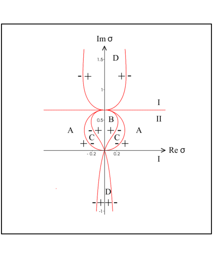
Fig. 1: Sign changes in S for $m=1,M=1,\Omega=1,\Lambda=6$.

The asymptotics near $\infty$ of $h_{03},h_{04}$ for $\sigma$ near and on the imaginary axis is surprising. Expected was that in the complement of imaginary axis there are always, both, a stable and an unstable solution of (63) and on the imaginary axis that both solutions are purely imaginary. Indeed this would have been the case if the second order term in this equation were absent. There one has either exponential growth of both solutions (in Regions D) or exponential decay of both solutions (Region B). As a consequence each $\sigma\in B$ – different from the values given in (60) – is an eigenvalue of $A$. Hence there is a continuum of eigenvalues for $A$ in the open left half-plane and hence the evolution given by (11), (3) and (13) is unstable.

7 Discussion and Open Problems

In the previous Section it was found that the spectrum of $\bar{A}$ contains a continuum of unstable eigenvalues leading to an unstable evolution given by (11), (3) and (13). In addition there was found a continuum of values $\sigma$ (from Regions D in Fig.1 – which include the spectral values found in the low-frequency approximation as well as (40) – for which any non trivial solution of the homogeneous equation corresponding to (31) growths exponentially near $\infty$. Hence it is to expect that those values are also part of the spectrum of $\bar{A}$ and hence contribute to the instability. Note in particular that their associated growth times displayed in Fig.1 can be of larger size than those for the found unstable eigenvalues (Region B in Fig.1) which suggests that the influence on the evolution dominantes over the influence of those eigenvalues.
A further question is how the constraint (15) – which has not been treated so far – is likely to influence the spectrum. The constraint should lead to closed subspace of $X$ being invariant under $\bar{A}$. Then the spectrum of the restriction of $\bar{A}$ to that subspace is a subset of the spectrum of $\bar{A}$. This should have the effect that the eigenvalues in region $B$ (see Fig.1) are becoming discrete instead whereas the continuous part of the spectrum in Region $D$ might be left unchanged, because in general continuous spectra are less sensitive to such a operation. In any case the singular structure of the resolvent at the values given by (40) will be unchanged having the effect that those values remain part of the spectrum at least when the system is restricted to finite space as is necessarily done in most numerical investigations. To decide these questions further study is needed. Note in this connection that the occurrence of an unbounded spectrum for $\bar{A}$ would not be a surprise, because for e.g., it is known that a self-adjoint operator has a bounded spectrum if and only if it is defined on the whole Hilbert space and in general differential operators cannot be defined on the whole of a weighted $L^{2}$-space. Also would the occurrence of an infinitely extended continuous part in the spectrum of oscillations be not surprising since that is quite common for infinitely extended physical systems.
From a physical point of view the main worrying feature of the results is their qualitative dependance on second order terms like that in (63). It is to expect that changes in second order to the coefficents in (11), (3) and (13) influence that term which can lead to a qualitative change of the spectrum. As a consequence different descriptions of the star which are equivalent to first order could lead to different statements on the stability of the star. Hence to decide that stability such corrections of the coefficients would have to be taken into account which in turn would lead to considering a changed operator. In addition judging from the mathematical mechanism how the coefficients of the evolution equations influence the spectrum – namely through the asymptotics of the homogeneous solutions of (31) near $\infty$ – it might be suspected that this property of the equations does not change in higher orders, which would ultimately question the expansion method as a proper means to investigate the stability of a rotating relativistic star. Also with respect to these points further study is necessary, but still the results raise first doubts whether the slow rotation approximation is appropriate for this purpose.
A final interesting question to ask is whether a numerical investigation of the evolution given by (11), (3) and (13) is capable of detecting the computed instabilities. This seems unlikely, because in that process space has to be ‘cutoff’ near the singular points $r=0,\infty$ and suitable local boundary conditions have to be posed at that the endpoints. But such a system is qualitatively different from the infinite system since for instance there the asymptotics of the homogeneous solutions (31) near $\infty$ does not play a role. Note that – independent from the used boundary conditions – for such a system the continuum of values given by the restriction of (40) to the chosen interval are part of the spectrum of the corresponding operator as also is also indicated by the numerical investigation [37].

Acknowledgements

I would like to thank Kostas Kokkotas and Johannes Ruoff for many important discussions. Also I would like to thank B. Schmidt for reading the paper and helpful suggestions.

8 Appendix

8.1 Conventions

The symbols ${\mathbb{N}}$, ${\mathbb{R}}$, ${\mathbb{C}}$ denote the natural numbers (including zero), all real numbers and all complex numbers, respectively.
To ease understanding we follow common abuse of notation and don’t differentiate between coordinate maps and coordinates. For instance, interchangeably $r$ will denote some real number greater than $0$ or the coordinate projection onto the open interval $I:=(0,\infty)$. The definition used will be clear from the context. In addition we assume composition of maps (which includes addition, multiplication etc.) always to be maximally defined. So for instance the addition of two maps (if at all possible) is defined on the intersection of the corresponding domains.
For each $k\in{\mathbb{N}}\setminus\{0\}$, $n\in{\mathbb{N}}\setminus\{0\}$ and each non-trivial open subset $M$ of ${\mathbb{R}}^{n}$ the symbol $C^{k}(M,{\mathbb{C}})$ denotes the linear space of $k$-times continuously differentiable complex-valued functions on $M$. Further $C^{k}_{0}(M,{\mathbb{C}})$ denotes the subspace of $C^{k}(M,{\mathbb{C}})$ consisting of those functions which in addition have a compact support in $\Omega$.
Throughout the paper Lebesgue integration theory is used in the formulation of [35]. Compare also Chapter III in [23] and Appendix A in [39]. To improve readability we follow common usage and don’t differentiate between an almost everywhere (with respect to the chosen measure) defined function $f$ and the associated equivalence class (consisting of all almost everywhere defined functions which differ from $f$ only on a set of measure zero). In this sense $L_{C}^{2}\left(M,\rho\right)$, where $\rho$ is some strictly positive real-valued continuous function on $M$, denotes the Hilbert space of complex-valued, square integrable (with respect to the measure $\rho\,d^{n}x$) functions on $M$. The scalar product $<|>$ on $L_{C}^{2}\left(M,\rho\right)$ is defined by

$$<f|g>:=\int_{M}f^{*}g\,\rho\,d^{n}x\,\,,$$ (80)

for all $f,g\in L_{C}^{2}\left(M,\rho\right)$, where ^∗ denotes complex conjugation on ${\mathbb{C}}$. It is a standard result of functional analysis that $C^{k}_{0}(M,{\mathbb{C}})$ is dense in $L_{C}^{2}\left(M,\rho\right)$.
Finally, throughout the paper standard results and nomenclature of operator theory is used. For this compare standard textbooks on Functional analysis, e.g.,[34] Vol. I, [35, 40].

8.2 Auxiliary Theorems

The variant of the theorem of Dunkel [16] (compare also [28, 6, 21]) used in Section 4 is the following.

Theorem 1

: Let $n\in N$; $a,t_{0}\in R$ with $a<t_{0}$; $\mu\in N$; $\alpha_{\mu}:=1$ for $\mu=0$ and $\alpha_{\mu}:=\mu$ for $\mu\neq 0$. In addition let $A_{0}$ be a diagonalizable complex $n\times n$ matrix and $e^{\prime}_{1},\dots,e^{\prime}_{n}$ be a basis of $C^{n}$ consisting of eigenvectors of $A_{0}$. Further, for each $j\in\{1,\cdots,n\}$ let $\lambda_{j}$ be the eigenvalue corresponding to $e^{\prime}_{j}$ and $P_{j}$ be the matrix representing the projection of $C^{n}$ onto $C.e^{\prime}_{j}$ with respect to the canonical basis of $C^{n}$. Finally, let $A_{1}$ be a continuous map from $(a,t_{0})$ into the complex $n\times n$ matrices $M(n\times n,C)$ for which there is a number $c\in(a,t_{0})$ such that the restriction of $A_{1jk}$ to $[c,t_{0})$ is Lebesgue integrable for each $j,k\in{1,...,n}$.

Then there is a $C^{1}$ map $R:(a,t_{0})\rightarrow M(n\times n,C)$ with $lim_{t\rightarrow 0}R_{jk}(t)=0$ for each $j,k\in{1,\dots,n}$ and such that $u:(a,t_{0})\rightarrow M(n\times n,C)$ defined by

$$u(t):=\left\{\begin{array}[]{ll}\sum^{n}_{j=1}(t_{0}-t)^{-\lambda_{j}}\cdot(E+R(t))\cdot P_{j}\ \mbox{for $\mu=0$}\cr\sum^{n}_{j=1}exp(\lambda_{j}(t_{0}-t)^{-\mu})\cdot(E+R(t))\cdot P_{j}\ \mbox{for $\mu\neq 0$ }\end{array}\right.\,$$ (83)

for all $t\in(a,t_{0})$ (where $E$ is the $n\times n$ unit matrix), maps into the invertible $n\times n$ matrices and satisfies

$$u^{\prime}(t)=\left(\frac{\alpha_{\mu}}{(t_{0}-t)^{\mu+1}}A_{0}+A_{1}(t)\right)\cdot u(t)$$ (84)

for each $t\in(a,t_{0})$.

Lemma 2

Let $X$ be a non-trivial Hilbert space with scalar product $<\,|\,>$ and induced norm $\|\,\|$ and let be $A:D(A)\rightarrow X$ a densely-defined, linear and closable operator in $X$. Further let be $\sigma\in{\mathbb{C}}$ such that $A-\sigma$ is injective. Finally, let be $\mu\in{\mathbb{C}^{*}}$ and let be $\eta_{0},\eta_{1},\dots$ a sequence of elements of $Ran(A-\sigma)$ for which there is an $\varepsilon\in(0,\infty)$ such that $\|\eta_{\nu}\|\geq\varepsilon$ for every $\nu\in{\mathbb{N}}$ and

$$\lim_{\nu\rightarrow\infty}\left[\left(A-\sigma\right)^{-1}\eta_{\nu}-\mu\eta_{\nu}\right]=0\,\,.$$ (85)

Then $\sigma+\mu^{-1}$ is in the spectrum of the closure $\bar{A}$ of $A$.

Proof: The proof is indirect. Assume otherwise that $\sigma+\mu^{-1}$ is not part of the spectrum of $\bar{A}$. Then $\bar{A}-(\sigma+\mu^{-1})$ is in particular bijective with a bounded inverse $\left(\bar{A}-(\sigma+\mu^{-1})\right)^{-1}$. Then we have for every $\nu\in{\mathbb{N}}$

$$\left(\bar{A}-(\sigma+\mu^{-1})\right)\left(A-\sigma\right)^{-1}\eta_{\nu}=\eta_{\nu}-\mu^{-1}\left(A-\sigma\right)^{-1}\eta_{\nu}$$ (86)

and hence also

$$\left(\bar{A}-(\sigma+\mu^{-1})\right)^{-1}\left(A-\sigma\right)^{-1}\eta_{\nu} = \mu\left(\bar{A}-(\sigma+\mu^{-1})\right)^{-1}\eta_{\nu}-$$ (87)

$$\mu\left(\bar{A}-\sigma\right)^{-1}\eta_{\nu}\,\,.$$

Using this it follows from (85) and the continuity of $\left(\bar{A}-(\sigma+\mu^{-1})\right)^{-1}$ that

$$\lim_{\nu\rightarrow\infty}\left\{\left(\bar{A}-(\sigma+\mu^{-1})\right)^{-1}\left(A-\sigma\right)^{-1}\eta_{\nu}-\mu\left(\bar{A}-(\sigma+\mu^{-1})\right)^{-1}\eta_{\nu}\right\}=$$

$$-\mu\lim_{\nu\rightarrow\infty}\left(A-\sigma\right)^{-1}\eta_{\nu}=0$$ (88)

and hence by (85) that

$$\lim_{\nu\rightarrow\infty}\eta_{\nu}=0\,\,.$$ (89)

The last is in contradiction to the assumption there is an $\varepsilon\in(0,\infty)$ such that $\|\eta_{\nu}\|\geq\varepsilon$ for all $\nu\in{\mathbb{N}}$. Hence the Lemma is proven._□

References

• [1] Andersson N 1998, A New Class of Unstable Modes of Rotating Relativistic Stars, ApJ, 502, 708-713.
• [2] Andersson N, Kokkotas K D 2001 The r-mode instability in rotating neutron stars, Int. J. Mod. Phys. D10, 381-442, gr-qc/0010102.
• [3] Andersson N, Kokkotas K D and Schutz B F 1999 Gravitational radiation limit on the spin of young neutron stars, ApJ, 510, 846-853.
• [4] Andersson N, Kokkotas K D and Stergioulas N 1999 On the relevance of the r-mode instability for accreting neutron stars and white Dwarfs, ApJ, 516, 307-314, gr-qc/0109065.
• [5] Balbinski E 1984, The continuous spectrum in differentially rotating perfect fluids - A model with an analytic solution, M.N.R.A.S., 209, 145-157.
• [6] Bellman R., 1949, A survey of the theory of the boundedness, stability, and asymptotic behaviour of solutions of linear and nonlinear differential and difference equations (Washington DC: NAVEXOS P-596, Office of Naval Research).
• [7] Beyer H R 1995 The spectrum of radial adiabatic stellar oscillations J. Math. Phys., 36, 4815-4825.
• [8] Beyer H R 1995 The spectrum of adiabatic stellar oscillations J. Math. Phys., 36, 4792-4814.
• [9] Beyer H R 2000 β€˜On some vector analogues of Sturm-Liouville operators’ in: Mathematical analysis and applications, T. M. Rassias (ed.), (Palm Harbor: Hadronic Press), 11-35.
• [10] Beyer H R and Kokkotas K D 1999 On the r-mode spectrum of relativistic stars Mon. Not. R. Astron. Soc., 308, 745-750.
• [11] Beyer H R and Schmidt B G 1995 Newtonian stellar oscillations Astron. Astrophys., 296, 722-726.
• [12] Chandrasekhar S 1981 Hydrodynamic and Hydromagnetic Stability (New York: Dover).
• [13] Chandrasekhar S 1970, Solutions of Two Problems in the Theory of Gravitational Radiation Phys. Rev. Lett., 24, 611-615.
• [14] Conway J B 1995 Functions of a complex variable I 2nd ed. (New York: Springer).
• [15] Drazin P G and Reid W H 1981 Hydrodynamic stability Cambridge: Cambridge University Press).
• [16] Dunkel O., 1912, Am. Acad. Arts Sci.Proc., 38, 341.
• [17] Friedman J L and Lockitch K H 2001, Implications of the r-mode instability of rotating relativistic stars, Review to appear in the proceedings of the 9th Marcel Grossman Meeting, World Scientific, ed. V. Gurzadyan, R. Jantzen, R. Ruffini, gr-qc/0102114.
• [18] Friedman J L and Schutz B F 1978 Secular instability of rotating newtonian stars ApJ, 222, 281-296.
• [19] Friedman J L and Morsink S 1998, Axial Instability of Rotating Relativistic Stars, ApJ, 502, 714-720.
• [20] Hartle J B 1967, Slowly Rotating Relativistic Stars: I. Equations of Structure, ApJ, 150, 1005-1029.
• [21] Hille E., 1969, Lectures on ordinary differential equations (Reading: Addison-Wesley).
• [22] Hille E and Phillips R S 1957 Functional Analysis and Semi-Groups (Providence: AMS).
• [23] Hirzebruch F and Scharlau W 1971 EinfΓΌhrung in die Funktionalanalysis (Mannheim: BI).
• [24] Joergens K 1964 Spectral Theory of Second-Order Ordinary Differential Operators Lectures delivered at Aarhus Universitet, (Mathematisk Institut Aarhus Universitet).
• [25] Kato T 1980 Perturbation Theory for Linear Operators (Berlin: Springer).
• [26] Kojima Y 1992 Equations governing the nonradial oscillations of a slowly rotating relativistic star Phys. Rev. D, 46, 4289-4303.
• [27] Kojima Y 1998 Quasi-toroidal oscillations in rotating relativistic stars Mon. Not. R. Astron. Soc., 293, 49-52.
• [28] Levinson N., 1948, Duke Math. J., 15, 111.
• [29] Lockitch K H, Andersson N, Friedman J L 2001 Rotational modes of relativistic stars: Analytic results, Phys. Rev. D, 63, 024019-1 - 024019-26.
• [30] Lindblom L, Owen B J and Morsink S M 1998 Gravitational radiation instability in hot young neutron stars, Phys. Rev. Lett., 80, 4843-4846.
• [31] Marden M 1989 Geometry of polynomials (Providence: AMS).
• [32] Misner C.W., Thorne K.S. and Wheeler J.A., 1973, Gravitation W.H.Freeman.
• [33] Owen B, Lindblom L, Cutler C, Schutz B F, Vecchio A. and Andersson N 1998, Gravitational waves from hot young rapidly rotating neutron stars Phys. Rev. D, 58, 084020-1 - 084020-15, gr-qc/9804044.
• [34] Reed M and Simon B 1980, 1975, 1979, 1978 Methods of Mathematical Physics Volume I, II, III, IV (New York: Academic).
• [35] Riesz F and Sz-Nagy B 1955 Functional Analysis (New York: Unger).
• [36] Ruoff J and Kokkotas K D 2001 On the r-mode spectrum of relativistic stars in the low-frequency approximation, M.N.R.A.S., 328, 678-688, gr-qc/0101105.
• [37] Ruoff J and Kokkotas K D 2002 On the r-mode spectrum of relativistic stars: Inclusion of the radiation reaction, MNRAS in press, gr-qc/0106073.
• [38] Schutz B F and Verdaguer E. 1983, Normal modes of Bardeen discs - II. A sequence of n=2 polytropes, M.N.R.A.S., 202, 881-901.
• [39] Weidmann J 1976 Lineare Operatoren in HilbertrΓ€umen (Teubner: Stuttgart).
• [40] Yosida K 1980 Functional Analysis (Berlin: Springer).