Oscillations of General Relativistic Superfluid Neutron Stars

Abstract

We develop a general formalism to treat, in general relativity, the nonradial oscillations of a superfluid neutron star about static (non-rotating) configurations. The matter content of these stars can, as a first approximation, be described by a two-fluid model: one fluid is the neutron superfluid, which is believed to exist in the core and inner crust of mature neutron stars; the other fluid is a conglomerate of all charged constituents (crust nuclei, protons, electrons, etcetera). We use a system of equations that governs the perturbations both of the metric and of the matter variables, whatever the equation of state for the two fluids. The entrainment effect is explicitly included. We also take the first step towards allowing for the superfluid to be confined to a part of the star by allowing for an outer envelope composed of ordinary fluid. We derive and implement the junction conditions for the metric and matter variables at the core/envelope interface, and briefly discuss the nature of the involved phase-transition. We then determine the frequencies and gravitational-wave damping times for a simple model equation of state, incorporating entrainment through an approximation scheme which extends present Newtonian results to the general relativistic regime. We investigate how the quasinormal modes of a superfluid star are affected by changes in the entrainment parameter, and unveil a series of avoided crossings between the various modes. We provide a proof that, unless the equation of state is very special, all modes of a two-fluid star must radiate gravitationally. We also discuss the future detectability of pulsations in a superfluid star and argue that it may be possible (given advances in the relevant technology) to use gravitational-wave data to constrain the parameters of superfluid neutron stars.

I Introduction

Ever since the realisation that Cepheids are stars undergoing radial pulsation ceph , the oscillation of stars has been an important research area. With much improved sensitivity, observations over the last few years have established a plethora of pulsating stars. The best case by far is provided by the Sun for which it is known sun that many high order pressure p-modes, and perhaps also the gravity g-modes and the Coriolis restored r-modes, are excited. By combining observational data with theoretical models researchers have been able to infer details of the Sun’s internal structure, e.g. the sound speed at different depths. These impressive results of so-called “helioseismology” provide inspiration for further research into stellar oscillations and the hope that “asteroseismology” astero will help further unveil details of the structure of distant stars. The purpose of this paper is to advance our modelling of non-radial oscillations of non-rotating, old and cold neutron stars that contain superfluid components.

Within the framework of general relativity oscillating compact stars provide an interesting potential source of gravitational radiation. There are several scenarios in which one would expect a neutron star to pulsate wildly, e.g. following its formation in a gravitational collapse, and it is interesting to ask whether the associated gravitational waves could be detected on Earth. Should this be the case, one can hope to use the gravitational-wave data to probe the star’s interior and possibly put constraints on the supranuclear equation of state astero1 ; astero2 .

In the last few years much attention has been focussed on gravitational-wave driven mode-instabilities in rapidly rotating stars. Ever since the seminal work of Chandrasekhar, Friedman and Schutz C70 ; F78 ; FS78 in the 1970s it has been known that gravitational waves can drive various modes of oscillation unstable, and recently it has been shown that the r-modes are particularly susceptible to the instability A98 ; FM98 . Most astrophysical r-mode scenarios regard hot young neutron stars, but it has also been proposed AKS99 that the instability may operate in mature accreting neutron stars, e.g. in Low-Mass X-ray binaries. These stars are expected to have core temperatures well below the superfluid transition temperature, and hence one would need to account for superfluidity in any detailed r-mode model. This is particularly important since mutual friction may provide a strong dissipative mechanism on any mode in a superfluid star mutual . In addition to this, it has been argued that the presence of a viscous boundary layer at the base of the crust of a mature neutron star will lead to a very strong damping on the r-modes ekman . While the issue of mutual friction has been discussed by Lindblom and Mendell LM00 , there are as yet no studies of dissipation due to a “realistic” core-crust interface, that is likely to involve the transition from a regime where superfluid neutrons co-exist with a lattice of crust nuclei to a region composed of superfluid neutrons and (possibly superconducting) protons.

Further motivation for our current work is provided by results from attempts to model the equation of state at supranuclear densities. Many modern equation of state calculations (within relativistic mean field theory) predict a sizeable hyperon fraction at high densities. However, the hyperons act as an effective “refrigerant” which means that the star would cool very fast. In fact, it has been argued that the presence of hyperons would lead to core temperatures well below those indicated by observations. The favoured resolution to this problem corresponds to the hyperons being superfluid. In addition, neutron stars may have cores composed of deconfined quarks which may also pair into exotic superfluid states. In other words, if we want to understand the dynamics of the core of a realistic mature neutron star we have to allow for one (or more) partially decoupled superfluid components.

The need for an improved understanding of these problems was recently emphasized by the suggestion that the presence of hyperons in the deep core would lead to a strong bulk viscosity wich could potentially completely suppress the unstable r-modes pbj ; lo01 . This suggestion brings may difficult issues to the top of the agenda. For example, a detailed study of unstable modes must necessarily account for the fact that a superfluid component(s) may move relative to the normal fluid component. One might expect this to have a significant effect on the estimates of time scales for an unstable mode. Furthermore, as has been pointed out by Andersson and Comer AC01a , one would expect new classes of r-modes (and indeed other inertial modes) to exist in a superfluid star. This means that the superfluid problem is likely to be richer than the ordinary, single fluid, one. Given that there have not yet been any detailed investigations into these issues it may be premature to draw any definite conclusions regarding the effect that superfluidity may have on mode-instabilities.

It is clear that a considerable amount of work on stars with one, or several, superfluid components remains to be done before we can claim to have an understanding of possible instabilities in mature neutron stars. These problems provide strong motivation for our current work.

Studies of oscillating superfluid stars were pioneered by Epstein E88 , who was the first to suggest that there ought to exist modes of oscillation that are unique to the superfluid case. These modes have since been calculated both in Newtonian theory LM94 ; L95 ; prix02 and general relativity CLL99 ; AC01b . It is now well established that a simple two-fluid model of a superfluid neutron star core has two families of fluid pulsation modes. The first of these is essentially the standard pressure p-modes, for which the two fluids tend to move together. The superfluid modes, on the other hand, are distinguished by the fact that the two fluids are counter-moving CLL99 ; AC01a . Another distinguishing characteristic of the superfluid modes is that their mode frequencies have a fundamental dependence on entrainment. Andersson and Comer AC01a have used a local analysis of the Newtonian superfluid equations to show that the modes are essentially acoustic in nature, with frequencies that depend on the stellar parameters as

$$\omega^{2}_{s}\approx{m_{p}\over m^{*}_{p}}{l(l+1)\over r^{2}}c^{2}_{p}\ ,$$ (1)

where $c_{p}$ is (roughly) the speed of sound in the proton fluid, $m_{p}$ and $m^{*}_{p}$ are the bare and effective proton masses, respectively, $r$ is the radial coordinate, and $l$ is the index of the relevant spherical harmonic $Y_{lm}(\theta,\phi)$. These results have recently been confirmed by detailed mode-calculations prix02 . The strong dependence of the superfluid modes on parameters that are difficult to constrain otherwise suggest a strategy that may be used in conjunction with future observations to narrow down the theoretical uncertainties AC01b . Specifically, an observational determination of the mode frequencies of an oscillating neutron star could be used to constrain the proton effective mass in dense nuclear matter. This would have immediate implications for BCS energy gap calculations since the effective mass is part of the required information (see, for instance, Khodel, Khodel, and Clark KKC01 ).

In this paper we concentrate on the equations that describe polar perturbations (even parity) of a general relativistic superfluid neutron star, using as our starting point the formalism developed by Comer, Langlois, and Lin CLL99 . The neutron star is assumed to consist of two distinct regions: a core consisting of matter in superfluid states, and an envelope of ordinary fluid matter. We report progress in three important directions. Firstly, we have obtained the first ever results for gravitational-wave damping rates of the superfluid oscillation modes. This is important as it allows us to assess the relevance of these modes for gravitational-wave astronomy. Secondly, we have developed a framework in which a superfluid region can be matched to an ordinary fluid region. (Lindblom & Mendell LM94 have employed a similar model in the Newtonian regime.) The introduction of an ordinary fluid envelope is the first step towards allowing for the presence of superfluids that are confined to distinct regions in the star. However, it is important to point out that since we do not incorporate elasticity in our model the envelope does not play the same role as the crust of a mature neutron star. In essence, our model corresponds to a star in which the fluid degrees of freedom contain a conglomerate “proton” fluid (consisting of nuclei and electrons in the envelope, and electrons and superconducting protons in the core) that extends from the surface to the center of the star and superfluid neutrons that exist only in the core. We work out the relevant junction/boundary conditions at the core/envelope interface and determine the quasinormal modes for such a neutron star model. Thirdly, we have included a simple model for the so-called entrainment effect, based on an explicit equation of state and an approximation that assumes that the fluid velocities are small compared to the speed of light. This allows us to provide the first detailed results describing the effect that entrainment has on the oscillation modes of a superfluid star. As we will show, this leads to the presence of so-called “avoided crossings” between neighbouring modes as the strength of entrainment is varied.

The main body of the paper begins with a discussion, in Sec. II, of the basic formalism used to describe non-radial, linearized oscillations of general relativistic superfluid neutron stars. This contains a discussion of the background, spherically symmetric and static equilibrium configurations, and the introduction of the variables that are used to model the non-radial oscillations. We also describe the key details of the numerical methods used to solve the linearized Einstein/superfluid field equations. The equation of state and inclusion of the entrainment effect are described in Sec. III, and the results of our numerical analysis are presented in Sec. IV. In Sec. V we prove that all pulsation modes of a superfluid star must radiate gravitational waves, unless the equation of state belongs to a very special class. Finally, we consider in Sec. VI the question of whether or not superfluid modes, excited, for instance, during a pulsar glitch, can be reliably extracted from gravitational-wave data. Some final remarks are offered in the concluding Sec. VII. For clarity of presentation and emphasis of the main physical results, we have relegated some of the formal, mathematical details to appendices. Appendix I is devoted to a derivation of the junction conditions used to tie together the core with the envelope. In Appendix II we present an analytical equation of state that can be used to incorporate the lowest-order effects of entrainment. Finally, in Appendix III a new method is presented which can be used to accurately determine long-lived quasinormal modes. We will be using geometrized units (except in Appendix II where the speed of light is restored) and “MTW” MTW conventions throughout the paper.

II Perturbations of superfluid stars

In this Section we summarise the equations that govern the equilibrium configurations of the superfluid core and the normal fluid envelope. What must be determined in the core are the neutron and proton number densities, and two metric coefficients. In the envelope only the proton number density remains but there are still two metric coefficients to specify. We also describe the complicated set of coupled linear perturbation equations that need to be integrated, and outline the computational strategy that we have adopted.

In what follows, the center of the star is at radial coordinate $r=0$, the core/envelope interface will be at $r=R_{c}$, and the surface at $r=R$.

II.1 General Relativistic Superfluid Formalism

The formalism to be used here, and motivation for it, has been described in great detail elsewhere CLL99 ; C89 ; CL94 ; CL95 ; CL98a ; CL98b ; LSC98 ; P00 ; AC01c . Hence, we will only mention the key features here. The central quantity of the superfluid formalism is the so-called master function $\Lambda$. It depends on the three scalars $n^{2}=-n_{\mu}n^{\mu}$, $p^{2}=-p_{\mu}p^{\mu}$ and $x^{2}=-p_{\mu}n^{\mu}$ that can be formed from the conserved neutron ($n^{\mu}$) and proton ($p^{\mu}$) number density currents. The master function is such that, when the two fluids are co-moving, $-\Lambda(n^{2},p^{2},x^{2})$ corresponds to the total thermodynamic energy density. Once the master function is provided (see Sec. IV for a simple analytic equation of state) the stress-energy tensor is given by

$$T^{\mu}_{\nu}=\Psi\delta^{\mu}_{\nu}+p^{\mu}\chi_{\nu}+n^{\mu}\mu_{\nu}\ ,$$ (2)

where

$$\Psi=\Lambda-n^{\rho}\mu_{\rho}-p^{\rho}\chi_{\rho}$$ (3)

is the generalised pressure, and

$$\mu_{\nu} = {\cal B}n_{\nu}+{\cal A}p_{\nu}\ ,$$ (4)

$$\chi_{\nu} = {\cal A}n_{\nu}+{\cal C}p_{\nu}\ ,$$ (5)

are the chemical potential covectors. We have also introduced

$${\cal A}=-{\partial\Lambda\over\partial x^{2}}\ ,\quad{\cal B}=-2{\partial\Lambda\over\partial n^{2}}\ ,\quad{\cal C}=-2{\partial\Lambda\over\partial p^{2}}\ .\quad$$ (6)

The momentum covectors $\mu_{\nu}$ and $\chi_{\nu}$ are dynamically, and thermodynamically, conjugate to $n^{\nu}$ and $p^{\nu}$. The two covectors also make manifest the so-called entrainment effect, that affects the dynamics of a superfluid neutron star in a crucial way. It is easy to see that the momentum of one constituent ($\mu_{\nu}$, say) carries along some of the mass current of the other constituent if ${\cal A}\neq 0$ (since $\mu_{\nu}$ is a linear combination of $n_{\nu}$ and $p_{\nu}$). On the other hand, if ${\cal A}=0$, i.e. if the master function does not depend on $x^{2}$, then there is no entrainment.

While the standard one-fluid problem can be expressed solely in terms of the Einstein equations, with the fluid equations of motion being automatically satisfied “by virtue of the Bianchi identities”, the two-fluid problem is different. Because of the additional dynamic degrees of freedom associated with the second fluid we need to use also (a subset of) the fluid equations of motion. The equations that need to be solved, in addition to the Einstein field equations, are two “continuity” equations

$$\nabla_{\mu}n^{\mu}=\nabla_{\mu}p^{\mu}=0\ .$$ (7)

These equations represent conservation of the superfluid neutrons and the protons separately. That is, we ignore “transfusion” from one component to the other due to, for example, weak interactions LSC98 . This is likely to be a reasonable approximation for the timescales and amplitudes that are relevant for nonradial pulsation. We also have two Euler-type equations

$$n^{\mu}\nabla_{[\mu}\mu_{\nu]}=p^{\mu}\nabla_{[\mu}\chi_{\nu]}=0\ .$$ (8)

II.2 Equilibrium models

In order to determine the background fluid configuration we need to evaluate the associated metric. We take our equilibrium configurations to be spherically symmetric and static, so the metric can be written in the Schwarzschild form

$$ds^{2}=-e^{\nu}dt^{2}+e^{\lambda}dr^{2}+r^{2}\left(d\theta^{2}+{\rm sin}^{2}\theta d\phi^{2}\right)\ .$$ (9)

The two metric coefficients are determined from two components of the Einstein equations, which can be written in the form

$$\lambda^{\prime}={1-e^{\lambda}\over r}-8\pi re^{\lambda}\Lambda\quad,\quad\nu^{\prime}=-{1-e^{\lambda}\over r}+8\pi re^{\lambda}\Psi\ ,$$ (10)

where a primes represents a radial derivative, and it is to be understood that $\Lambda=\Lambda(n,p)$ and $\Psi=\Psi(n,p)$ in the interval $0\leq r\leq R_{c}$ and $\Lambda=\Lambda(p)$ and $\Psi=\Psi(p)$ in the interval $R_{c}\leq r\leq R$.

The equations that determine the radial profiles of $n(r)$ and $p(r)$ in the core have been derived in Comer, Langlois, and Lin CLL99 . They follow from (8), and can be written

$${\cal A}^{0}_{0}p^{\prime}+{\cal B}^{0}_{0}n^{\prime}+{1\over 2}({\cal B}n+Ap)\nu^{\prime}=0\quad,\quad{\cal C}^{0}_{0}p^{\prime}+{\cal A}^{0}_{0}n^{\prime}+{1\over 2}({\cal C}p+{\cal A}n)\nu^{\prime}=0\ ,$$ (11)

where

$${\cal A}_{0}^{0} = {\cal A}+2{\partial{\cal B}\over\partial p^{2}}np+2{\partial{\cal A}\over\partial n^{2}}n^{2}+2{\partial{\cal A}\over\partial p^{2}}p^{2}+{\partial{\cal A}\over\partial x^{2}}pn\ ,$$ (12)

$${\cal B}_{0}^{0} = {\cal B}+2{\partial{\cal B}\over\partial n^{2}}n^{2}+4{\partial{\cal A}\over\partial n^{2}}np+{\partial{\cal A}\over\partial x^{2}}p^{2},$$ (14)

$${\cal C}_{0}^{0} = {\cal C}+2{\partial{\cal C}\over\partial p^{2}}p^{2}+4{\partial{\cal A}\over\partial p^{2}}np+{\partial A\over\partial x^{2}}n^{2}\ .$$ (16)

In the coefficients above, one sets $x^{2}=np$ after the partial derivatives are taken for the equilibrium configuration.

For the particular model equation of state we use in our numerical calculations, the above equations require that the two fluids have a common surface (i.e. $n\to 0$ as $p\to 0$) if one assumes chemical equilibrium. The oscillations of such models were studied in CLL99 . Here we want to consider models such that the two-fluid regime is enclosed within a single fluid envelope. It is easy to build such a model by relaxing the assumption of chemical equilibrium in the core. The resultant models are likely not too unrealistic given the relatively long timescales required for nuclear interactions to reinstate equilibrium.

Our models are such that the superfluid neutron number density is zero in the envelope, and thus the only matter equation is

$${\cal C}^{0}_{0}p^{\prime}+{1\over 2}Cp\nu^{\prime}=0\ ,$$ (17)

where now

$${\cal C}=-2{\partial\Lambda\over\partial p^{2}}\quad,\quad{{\cal C}_{0}^{0}}={\cal C}+2p^{2}{\partial{\cal C}\over\partial p^{2}}\ .$$ (18)

There are three sets of “boundary” conditions that must be dealt with: a set at the center, one at the interface, and the remaining one at the surface of the star. In view of Eq. (10), requiring a non-singular behavior at the center of the star will impose that $\lambda(0)=0$, and consequently $\lambda^{\prime}(0)$ and $\nu^{\prime}(0)$ must also vanish. This in turn implies, in view of Eq. (11), that $p^{\prime}(0)$ and $n^{\prime}(0)$ have to vanish as well. Although our analysis of the junction conditions at the interface allows for other possibilities, our numerical calculations assume that the phase transition that leads to the formation of superfluid neutrons is second order. In other words, we consider the energy density to be continuous at $R_{c}$. From the analysis presented in Appendix I, we see that the two metric coefficients and the pressure must then also be continuous. We will also assume that the proton number density and the proton chemical potential are continuous at the interface. At the surface, we will only consider configurations that satisfy $p(R)=0$. A smooth joining of the interior spacetime to a Schwarzschild vacuum exterior at the surface of the star implies that the total mass $M$ of the system is given by

$$M=-4\pi\int^{R}_{0}r^{2}~{}\Lambda(r)dr$$ (19)

and that $\Psi(R)=0$.

II.3 The linearized field equations

It is well-known that all non-trivial pulsation modes of a nonrotating fluid star correspond to polar pertubations (often referred to as “even parity”). In the so-called Regge-Wheeler gauge RW , the corresponding metric components are

$$\delta g_{\mu\nu}=-e^{i\omega t}\left[\matrix{e^{\nu}r^{l}H_{0}(r)&i\omega r^{l+1}H_{1}(r)&0&0\cr i\omega r^{l+1}H_{1}(r)&e^{\lambda}r^{l}H_{0}(r)&0&0\cr 0&0&r^{l+2}K(r)&0\cr 0&0&0&r^{l+2}{\rm sin}^{2}\theta K(r)}\right]P_{l}(\theta)\ .$$ (20)

where $P_{l}(\theta)$ are the Legendre polynomials. This decomposition will be applied to both the core and the envelope.

Writing the neutron and proton four-currents as $n^{\mu}=nu^{\mu}$ and $p^{\mu}=pv^{\mu}$, where $u_{\mu}u^{\mu}=-1$ and $v_{\mu}v^{\mu}=-1$, one can show that in the core the independent components are

$$\delta u^{i}=e^{-\nu/2}{\partial\over\partial t}\delta\xi^{i}_{n}\quad,\quad\delta v^{i}=e^{-\nu/2}{\partial\over\partial t}\delta\xi^{i}_{p}\ ,$$ (21)

where

$$\delta\xi_{n}^{r}=e^{-\lambda/2}r^{l-1}{W_{n}}(r)P_{l}e^{i\omega t}\quad,\quad\delta\xi_{n}^{\theta}=-r^{l-2}{V_{n}}(r){\partial\over\partial\theta}P_{l}e^{i\omega t}\ ,$$ (22)

and

$$\delta\xi_{p}^{r}=e^{-\lambda/2}r^{l-1}{W_{p}}(r)P_{l}e^{i\omega t}\quad,\quad\delta\xi_{p}^{\theta}=-r^{l-2}{V_{p}}(r){\partial\over\partial\theta}P_{l}e^{i\omega t}\ .$$ (23)

The Lagrangian variations in the neutron and proton number densities can be written as, respectively,

$${\Delta n\over n} = \delta n+n^{\prime}e^{-\lambda/2}r^{l-1}W_{n}\ ,$$ (24)

$${\Delta p\over p} = \delta p+p^{\prime}e^{-\lambda/2}r^{l-1}W_{p}\ ,$$ (26)

and the conservation equations (7) for the particle number currents yield

$${\Delta n\over n} = -r^{l}\left(e^{-\lambda/2}\left[{l+1\over r^{2}}W_{n}+{1\over r}W^{\prime}_{n}\right]+{l(l+1)\over r^{2}}V_{n}-{1\over 2}H_{0}-K\right)\ ,$$ (27)

$${\Delta p\over p} = -r^{l}\left(e^{-\lambda/2}\left[{l+1\over r^{2}}W_{p}+{1\over r}W^{\prime}_{p}\right]+{l(l+1)\over r^{2}}V_{p}-{1\over 2}H_{0}-K\right)\ .$$ (29)

Thus, all matter variables can be expressed in terms of the velocity variables $W_{n,p}$ and $V_{n,p}$. In the envelope, we have as the only independent matter variables ${W_{p}}$ and ${V_{p}}$.

The set of perturbation equations that we solve for in the superfluid core have already been listed in CLL99 , but since our core/envelope problem requires a slightly different method of solution we repeat the relevant equations here. We also need these equations for the analysis in Section V.

First we define (in analogy with Lindblom and Detweiler’s LD ; DL approach to the one-fluid problem) two new variables as

$${X_{n}}\equiv n\left[{e^{\nu/2}\over 2}\mu{H_{0}}+e^{-\nu/2}\omega^{2}\left({\cal B}n{V_{n}}+{\cal A}p{V_{p}}\right)\right]-e^{(\nu-\lambda)/2}{n^{\prime}\over r}\left({{\cal B}_{0}^{0}}n{W_{n}}+{{\cal A}_{0}^{0}}p{W_{p}}\right)\ ,$$ (30)

and

$${X_{p}}\equiv p\left[{e^{\nu/2}\over 2}\chi{H_{0}}+e^{-\nu/2}\omega^{2}\left({\cal C}p{V_{p}}+{\cal A}n{V_{n}}\right)\right]-e^{(\nu-\lambda)/2}{p^{\prime}\over r}\left({{\cal C}_{0}^{0}}p{W_{p}}+{{\cal A}_{0}^{0}}n{W_{n}}\right)\ .$$ (31)

Then we find that the Einstein and superfluid field equations yield an algebraic constraint equation

$$e^{\lambda}\left[{2-l-l^{2}\over r^{2}}-{3\over r^{2}}\left(1-e^{-\lambda}\right)-8\pi\Psi\right]{H_{0}}+\left[{2\omega^{2}\over e^{\nu}}-{l(l+1)\over 2}e^{\lambda}\left({1-e^{-\lambda}\over r^{2}}+8\pi\Psi\right)\right]{H_{1}}$$ (32)

$$+\left[-2e^{\lambda-\nu}\omega^{2}+e^{\lambda}{l^{2}+l-2\over r^{2}}+e^{2\lambda}\left({1-e^{-\lambda}\over r^{2}}+8\pi\Psi\right)\left(1-{3\over 2}\left(1-e^{-\lambda}\right)-4\pi r^{2}\Psi\right)\right]K$$ (33)

$$+16\pi e^{\lambda-\nu/2}\left({X_{n}}+{X_{p}}\right)=0\ ,$$ (34)

and a system of coupled ordinary differential equations (where we use the definition ${{\cal D}_{0}^{0}}={{\cal B}_{0}^{0}}{{\cal C}_{0}^{0}}-({{\cal A}_{0}^{0}})^{2}$):

$${H_{1}}^{\prime} = {e^{\lambda}\over r}{H_{0}}+\left[{\lambda^{\prime}-\nu^{\prime}\over 2}-{l+1\over r}\right]{H_{1}}+{e^{\lambda}\over r}K-16\pi{e^{\lambda}\over r}\left(\mu n{V_{n}}+\chi p{V_{p}}\right)\ ,$$ (35)

$$K^{\prime} = {{H_{0}}\over r}+{l(l+1)\over 2r}{H_{1}}+\left[{\nu^{\prime}\over 2}-{l+1\over r}\right]K-8\pi{e^{\lambda/2}\over r}\left[\mu n{W_{n}}+\chi p{W_{p}}\right]\ ,$$ (37)

$${W_{n}}^{\prime} = {e^{\lambda/2}r\over 2}{H_{0}}+e^{\lambda/2}rK-e^{\lambda/2}{l(l+1)\over r}{V_{n}}-\left({l+1\over r}+{n^{\prime}\over n}\right){W_{n}}+$$ (41)

$$+{{{\cal C}_{0}^{0}}\over n^{2}{{\cal D}_{0}^{0}}}\left[e^{(\lambda-\nu)/2}r{X_{n}}+n^{\prime}\left({{\cal B}_{0}^{0}}n{W_{n}}+{{\cal A}_{0}^{0}}p{W_{p}}\right)\right]-$$

$${{{\cal A}_{0}^{0}}\over np{{\cal D}_{0}^{0}}}\left[e^{(\lambda-\nu)/2}r{X_{p}}+p^{\prime}\left({{\cal A}_{0}^{0}}n{W_{n}}+{{\cal C}_{0}^{0}}p{W_{p}}\right)\right]\ ,$$

$${W_{p}}^{\prime} = {e^{\lambda/2}r\over 2}{H_{0}}+e^{\lambda/2}rK-e^{\lambda/2}{l(l+1)\over r}{V_{p}}-\left({l+1\over r}+{p^{\prime}\over p}\right){W_{p}}$$ (45)

$$+{{{\cal B}_{0}^{0}}\over p^{2}{{\cal D}_{0}^{0}}}\left[e^{(\lambda-\nu)/2}r{X_{p}}+p^{\prime}\left({{\cal C}_{0}^{0}}p{W_{p}}+{{\cal A}_{0}^{0}}n{W_{n}}\right)\right]-$$

$${{{\cal A}_{0}^{0}}\over np{{\cal D}_{0}^{0}}}\left[e^{(\lambda-\nu)/2}r{X_{n}}+n^{\prime}\left({{\cal A}_{0}^{0}}p{W_{p}}+{{\cal B}_{0}^{0}}n{W_{n}}\right)\right]\ ,$$

$${X_{n}}^{\prime} = -{l\over r}{X_{n}}+{e^{\nu/2}\over 2}\left[n\mu\left({1\over r}-\nu^{\prime}\right)-n^{\prime}\left({{\cal B}_{0}^{0}}n+{{\cal A}_{0}^{0}}p\right)\right]{H_{0}}$$ (52)

$$+\mu n\left[{e^{\nu/2}\over 4}{l(l+1)\over r}+{\omega^{2}\over 2}re^{-\nu/2}\right]{H_{1}}$$

$$+e^{\nu/2}\left[\mu n\left({\nu^{\prime}\over 4}-{1\over 2r}\right)-\left({{\cal B}_{0}^{0}}n+{{\cal A}_{0}^{0}}p\right)n^{\prime}\right]K+{l(l+1)\over r^{2}}e^{\nu/2}n^{\prime}\left({{\cal B}_{0}^{0}}n{V_{n}}+{{\cal A}_{0}^{0}}p{V_{p}}\right)$$

$$-e^{(\lambda-\nu)/2}{\omega^{2}\over r}n\left({\cal B}n{W_{n}}+{\cal A}p{W_{p}}\right)-4\pi e^{(\lambda+\nu)/2}{\mu n\over r}\left(\mu n{W_{n}}+\chi p{W_{p}}\right)$$

$$+e^{-(\lambda-\nu)/2}\left[-{n^{\prime}\over r}\left({{\cal B}_{0}^{0}}^{\prime}n{W_{n}}+{{\cal A}_{0}^{0}}^{\prime}p{W_{p}}\right)+\left({2n^{\prime}\over r^{2}}+{\lambda^{\prime}-\nu^{\prime}\over 2r}n^{\prime}-{n^{\prime\prime}\over r}\right)\right.$$

$$\left.\left({{\cal B}_{0}^{0}}n{W_{n}}+{{\cal A}_{0}^{0}}p{W_{p}}\right)\right]\ ,$$

$${X_{p}}^{\prime} = -{l\over r}{X_{p}}+{e^{\nu/2}\over 2}\left[p\chi\left({1\over r}-\nu^{\prime}\right)-p^{\prime}\left({{\cal C}_{0}^{0}}p+{{\cal A}_{0}^{0}}n\right)\right]{H_{0}}$$ (59)

$$+\chi p\left[{e^{\nu/2}\over 4}{l(l+1)\over r}+{\omega^{2}\over 2}re^{-\nu/2}\right]{H_{1}}$$

$$+e^{\nu/2}\left[\chi p\left({\nu^{\prime}\over 4}-{1\over 2r}\right)-\left({{\cal C}_{0}^{0}}p+{{\cal A}_{0}^{0}}n\right)p^{\prime}\right]K+{l(l+1)\over r^{2}}e^{\nu/2}p^{\prime}\left({{\cal C}_{0}^{0}}p{V_{p}}+{{\cal A}_{0}^{0}}n{V_{n}}\right)$$

$$-e^{(\lambda-\nu)/2}{\omega^{2}\over r}p\left({\cal C}p{W_{p}}+{\cal A}n{W_{n}}\right)-4\pi e^{(\lambda+\nu)/2}{\chi p\over r}\left(\chi p{W_{p}}+\mu n{W_{n}}\right)$$

$$+e^{-(\lambda-\nu)/2}\left[-{p^{\prime}\over r}\left({{\cal C}_{0}^{0}}^{\prime}p{W_{p}}+{{\cal A}_{0}^{0}}^{\prime}n{W_{n}}\right)+\left({2p^{\prime}\over r^{2}}+{\lambda^{\prime}-\nu^{\prime}\over 2r}p^{\prime}-{p^{\prime\prime}\over r}\right)\right.$$

$$\left.\left({{\cal C}_{0}^{0}}p{W_{p}}+{{\cal A}_{0}^{0}}n{W_{n}}\right)\right]\ .$$

The equations for the ordinary fluid envelope are obtained by taking the $n=0$ limit of the field equations. It is, however, not quite as straightforward as letting $n\to 0$ in the above set of two-fluid perturbation equations. The reason for this is that we have in places divided through by ${{\cal D}_{0}^{0}}$ which vanishes in the one-fluid limit.

In the one-fluid case, the constraint equation becomes

$$e^{\lambda}\left[{2-l-l^{2}\over r^{2}}-{3\over r^{2}}\left(1-e^{-\lambda}\right)-8\pi\Psi\right]{H_{0}}+\left[{2\omega^{2}\over e^{\nu}}-{l(l+1)\over 2}e^{\lambda}\left({1-e^{-\lambda}\over r^{2}}+8\pi\Psi\right)\right]{H_{1}}$$ (60)

(61)

$$+\left[-2e^{\lambda-\nu}\omega^{2}+e^{\lambda}{l^{2}+l-2\over r^{2}}+e^{2\lambda}\left({1-e^{-\lambda}\over r^{2}}+8\pi\Psi\right)\left(1-{3\over 2}\left(1-e^{-\lambda}\right)-4\pi r^{2}\Psi\right)\right]K$$ (62)

(63)

$$+16\pi e^{\lambda-\nu/2}{X_{p}}=0\ .$$ (64)

The other two equations for the metric are

$${H_{1}}^{\prime} = {e^{\lambda}\over r}{H_{0}}+\left[{\lambda^{\prime}-\nu^{\prime}\over 2}-{l+1\over r}\right]{H_{1}}+{e^{\lambda}\over r}K-16\pi{e^{\lambda}\over r}\chi p{V_{p}}\ ,$$ (65)

$$K^{\prime} = {{H_{0}}\over r}+{l(l+1)\over 2r}{H_{1}}+\left[{\nu^{\prime}\over 2}-{l+1\over r}\right]K-8\pi{e^{\lambda/2}\over r}\chi p{W_{p}}\ .$$ (67)

The final two equations are for the fluid and they take the form

$${W_{p}}^{\prime} = {e^{\lambda/2}r\over 2}{H_{0}}+e^{\lambda/2}rK-e^{\lambda/2}{l(l+1)\over r}{V_{p}}-{l+1\over r}{W_{p}}+{e^{(\lambda-\nu)/2}r\over p^{2}{{\cal C}_{0}^{0}}}{X_{p}}\ ,$$ (68)

$${X_{p}}^{\prime} = -{l\over r}{X_{p}}+{e^{\nu/2}\over 2}\left[p\chi\left({1\over r}-\nu^{\prime}\right)-p^{\prime}{{\cal C}_{0}^{0}}p\right]{H_{0}}+\chi p\left[{e^{\nu/2}\over 4}{l(l+1)\over r}+{\omega^{2}\over 2}re^{-\nu/2}\right]{H_{1}}$$ (76)

$$+e^{\nu/2}\left[\chi p\left({\nu^{\prime}\over 4}-{1\over 2r}\right)-{{\cal C}_{0}^{0}}pp^{\prime}\right]K+{l(l+1)\over r^{2}}e^{\nu/2}p^{\prime}{{\cal C}_{0}^{0}}p{V_{p}}$$

$$-e^{(\lambda-\nu)/2}{\omega^{2}\over r}{\cal C}p^{2}{W_{p}}-4\pi e^{(\lambda+\nu)/2}{(\chi p)^{2}\over r}{W_{p}}$$

$$+e^{-(\lambda-\nu)/2}\left[-{p^{\prime}\over r}{{\cal C}_{0}^{0}}^{\prime}p{W_{p}}+\left({2p^{\prime}\over r^{2}}+{\lambda^{\prime}-\nu^{\prime}\over 2r}p^{\prime}-{p^{\prime\prime}\over r}\right){{\cal C}_{0}^{0}}p{W_{p}}\right]\ ,$$

where

$${X_{p}}=p\left[{e^{\nu/2}\over 2}\chi{H_{0}}+e^{-\nu/2}\omega^{2}\left({\cal C}p{V_{p}}\right)\right]-e^{(\nu-\lambda)/2}{p^{\prime}\over r}\left({{\cal C}_{0}^{0}}p{W_{p}}\right)\ .$$ (77)

This set of equations is identical to that previously used DL ; LD to study the oscillations of normal fluid neutron stars for a range of supranuclear equations of state.

At the center of the star, the conditions are those given in Appendix A of Comer, Langlois, and Lin CLL99 , i.e. all functions are regular. At the surface, the conditions are the one-fluid conditions used by Detweiler and Lindblom DL ; LD . The main difference here concerns the interface. The detailed treatment of the interface is discussed in Appendix I. It is found that the relativistic junction conditions imply that the three metric perturbations $H_{0},H_{1}$ and $K$ must be continuous at the interface. We assume that $W_{n}(R_{c})$ is free to vary at the interface, i.e., the value it takes at the interface is determined by the general solution produced for the core. We also assume that ${X_{n}}(R_{c})=0$, which will be shown below to be consistent with the chosen equation of state. From the results presented in Appendix I, it is found that two conditions remain. One of these implies that ${X_{p}}$ must be continuous at the interface. Recalling that we assume the proton number density and proton chemical potential to be continuous at the interface, i.e. that we have a second order phase-transition, the last condition is that ${W_{p}}$ must also be continuous at the interface.

II.4 Computational strategy

Even though our strategy for integrating the perturbation equations is similar to that used by Comer, Langlois, and Lin CLL99 there are some subtleties associated with the presence of the one-fluid envelope. Hence, it is worthwhile outlining the approach we have taken to the problem. In the core the perturbation equations can be written as the matrix equation

$${d{\bf Y}\over dr}={\bf Q}\cdot{\bf Y}\ ,$$ (78)

where

$${\bf Y}=\{H_{1},K,W_{n},W_{p},X_{n},X_{p}\}$$ (79)

is an abstract six-dimensional vector field. The $6\times 6$ matrix ${\bf Q}$ depends on $l$, $\omega$, the background fields, and the various coefficients ${\cal A}$, ${{\cal A}_{0}^{0}}$, etc. As was shown by Comer, Langlois, and Lin one need only specify the set of values $\{K(0),{W_{n}}(0),{W_{p}}(0)\}$ at the center of the star. The remaining variables, $H_{1}(0)$, ${X_{n}}(0)$, and ${X_{p}}(0)$, then follow from the $r\to 0$ limit of the perturbation equations. All of the second derivatives, $H_{1}^{\prime\prime}(0)$, $K^{\prime\prime}(0)$, etc, are likewise determined by $\{K(0),{W_{n}}(0),{W_{p}}(0)\}$. This means that, in order to provide information that enables us to construct the general solution, an integration starting from the centre must generate three linearly independent solutions ${\bf Y}_{1}$, ${\bf Y}_{2}$, and ${\bf Y}_{3}$. The corresponding general solution can thus be written

$${\bf Y}(r)=\sum^{3}_{i=1}c_{i}{\bf Y}_{i}(r)\ ,$$ (80)

where the $c_{i}$ ($i=1,2,3$) are constants to be determined.

In the envelope, the problem is equivalent to the standard one for a single fluid and our strategy is identical to that of Lindblom and Detweiler DL ; LD . We write the perturbation equations as

$${d{\bf\tilde{Y}}\over dr}={\bf\tilde{Q}}\cdot{\bf\tilde{Y}}\ ,$$ (81)

where

$${\bf\tilde{Y}}=\{H_{1},K,W_{p},X_{p}\}$$ (82)

and the matrix ${\bf\tilde{Q}}$ can be deduced from Eqns. (64)–(76). At the surface of the star our solution must satisfy the single condition $X_{p}(R)=0$ (cf. DL ; LD ). This means that we must generate three linearly independent solutions in the envelope and the general solution can therefore be written

$${\bf\tilde{Y}}(r)=\sum^{6}_{i=4}c_{i}{\bf\tilde{Y}}_{i}(r)\ .$$ (83)

At the core/envelope interface we must enforce the additional condition that $X_{n}(R_{c})=0$. We also know, from the analysis in Appendix I, that the variables $H_{1}$, $K$, $W_{p}$ and $X_{p}$ should all be continuous across the interface. This means that only the function value $W_{n}(R_{c})$ remains unspecified. This is, however, as it should be since the interface represents a “free boundary” for the superfluid neutrons. (An analogy can be made with the water/air interface of the oceans, where the water oscillation is free at the interface.) Our strategy for solving the problem is based on two steps. First we continue the three solutions from the envelope into the core assuming in addition that $W_{n}(R_{c})=0$. Then we determine a fourth solution (needed to generate the general solution in the core) by assuming that $W_{n}(R_{c})\neq 0$, but that all the other variables vanish at the interface. This means that we have determined a general solution of form

$${\bf Y}(r)=\sum^{7}_{i=4}c_{i}{\bf Y}_{i}(r)\ ,$$ (84)

where ${\bf Y}_{i}(R_{c})={\bf\tilde{Y}}_{i}(R_{c})$ for $i=4-6$.

The remaining step is to match the various solutions at some point $r=r_{m}$ in the core $0\leq r_{m}\leq R_{c}$. At $r_{m}$ we must have

$$\sum^{3}_{i=1}c_{i}{\bf Y}_{i}(r_{m})=\sum^{7}_{i=4}c_{i}{\bf Y}_{i}(r_{m})\ .$$ (85)

Once we have provided the overall normalisation (by specifying one of the $c_{i}$ coefficients), this problem can readily be solved for the remaining coefficients. This completes the solution of the interior problem.

To determine the global solution we must also solve for the exterior metric perturbations. This problem reduces to that of integrating the Zerilli equation, cf. CLL99 . Finally, in order to find a quasinormal mode (QNM) of the system we need to identify solutions that correspond to purely outgoing waves at spatial infinity. Our method for determining long-lived QNMs is described in Appendix III.

III An Analytical Entrainment Model

In order to extend the previous work by Comer, Langlois, and Lin CLL99 further we want to construct a sensible equation of state that incorporates the entrainment effect. This effect arises whenever there is a coupling between two interpenetrating fluids, and has the net result that the momentum of one fluid is not simply proportional to that fluid’s velocity. Rather, it is a linear combination of the velocities of both fluids. Hence, when one constituent starts to flow it will necessarily induce a momentum in the other. However, the entrainment effect is poorly understood, and there are as yet no completed relativistic models that we can base our discussion on. (The problem is currently being considered by Comer and Joynt, and we are hopeful that a fully relativistic formalism will soon be available.) The involved microphysics is, in fact, so uncertain that the best strategy corresponds to introducing some convenient parameterisation and then studying whether a variation in the chosen parameters affects the overall properties of the star and/or it’s modes of pulsation.

We noted earlier, in Sec. II, that the two chemical potential covectors $\mu_{\mu}$ and $\chi_{\mu}$ make manifest the entrainment effect by being linear combinations of the conserved four-currents, $n^{\mu}$ and $p^{\mu}$. Ultimately, this traces back to the master function $\Lambda$ depending explicitly on the “entrainment variable” $x^{2}$. Its presence in the background and perturbation equations listed in Sec. II is most apparent through the values of the coefficients ${\cal A}$ and ${\cal A}_{0}^{0}$. In the following we will use an expansion in terms of $x^{2}$ as outlined in Appendix II. At the heart of this expansion are the dimensionless ratios of the neutron and proton three-velocities with respect to the speed of light. This expansion makes sense since one would expect these ratios to be extremely small under most circumstances. Then the expansion becomes particularly accurate. The equation of state so constructed should have applications to the studies of quasinormal modes of neutron stars, with both static spherically symmetric and slowly rotating backgrounds. We thus expand the master function as

$$\Lambda(n^{2},p^{2},x^{2})=\sum_{i=0}^{\infty}\lambda_{i}(n^{2},p^{2})\left(x^{2}-np\right)^{i}\ ,$$ (86)

where $x^{2}-np$ is expected to be small with respect to $np$. It should be noted that there are combinations other than $x^{2}-np$ that could be used in the expansion, the most obvious being those that have no dimensions, say, $(x^{2}-np)/np$. These combinations are, however, not convenient in that the ${\cal A}$, ${\cal B}$, etc coefficients require that partial derivatives with respect to $n^{2}$ and $p^{2}$ be taken. The effect of this is that the expansions for ${\cal A}$, ${\cal B}$, etc would then not take the same form as Eq. (86) above, since every derivative would bring in extra factors of $x^{2}$ outside the terms $[(x^{2}-np)/np]^{i}$. A quick glance at Appendix II will show that if we use an expansion based on $x^{2}-np$ the basic form of the expansion is preserved for all coefficients that enter the field equations.

In order to make contact with previous Newtonian studies of oscillating superfluid stars we will adopt the particular entrainment model used by Lindblom and Mendell LM00 . To do this, a point of connection must be made between the coefficients used in the general relativistic superfluid equations and the corresponding Newtonian equations. This connection can be made by taking the Newtonian limit of the general relativistic superfluid formalism and then comparing the dynamical variables (as in AC01a ). In this way the mass matrix components $\rho_{nn}$, $\rho_{pp}$, and $\rho_{np}$ of the Newtonian formalism (cf. AB75 ) can be directly connected to the analytical entrainment coefficient $\lambda_{1}$ of the general relativistic formalism (cf. Appendix II) and the particle number densities $n$ and $p$. Following this strategy we find that $\lambda_{1}$ can be written as

$$\lambda_{1}=-{c^{2}m_{n}m_{p}\over\rho_{np}^{2}-\rho_{nn}\rho_{pp}}\rho_{np}\ ,$$ (87)

where

$$m_{n}n=\rho_{nn}+\rho_{np}\quad,\quad m_{p}p=\rho_{pp}+\rho_{np}\ .$$ (88)

where $m_{n(p)}$ is the neutron (proton) mass. The particular model of Lindblom and Mendell LM00 sets

$$\rho_{np}=-\epsilon m_{n}n\ ,$$ (89)

where $\epsilon$ is a constant. In the following we will refer to $\epsilon$ as the “entrainment parameter.” From the analysis of Prix, Comer and Andersson PCA01 one can infer that

$$\epsilon={m_{p}p\over m_{n}n}\left({m_{p}\over m^{*}_{p}}-1\right)\ ,$$ (90)

where $m^{*}_{p}$ is the proton effective mass. Given that $0.3\leq m^{*}_{p}/m_{p}\leq 0.8$ (see, for instance, Sjöberg S76 ) “typical” values for a neutron star core may lie in the range $0.04\leq\epsilon\leq 0.2$. In the following we take this range as being “physically reasonable”.

At this point it is relevant to note that, after all the numerical work described in this paper had been completed, Prix et al PCA01 developed an alternative description of entrainment. While we could, in principle, have adopted our formulas here to this new description we have decided not to do this. Such a change would not have affected our discussion or the implications of our results in any way.

IV Numerical results

IV.1 An analytical equation of state

We will now apply our formalism to a simple model equation of state. We consider the case where each core fluid (at the lowest order in the expansion presented in Appendix II) behaves as a relativistic polytrope, i.e. we take

$$\lambda_{0}(n^{2},p^{2})=-m_{n}n-\sigma_{n}n^{\beta_{n}}-m_{p}p-\sigma_{p}p^{\beta_{p}}\ .$$ (91)

This master function is clearly separable in $n$ and $p$. Using the formalism developed in Appendix II, the relevant coefficients are (for the equilibrium configurations where $x^{2}=np$)

$${\cal A}=\epsilon{m_{n}m_{p}\over m_{p}p+\epsilon(m_{n}n+m_{p}p)}\quad,\quad{{\cal A}_{0}^{0}}=0\ ,$$ (92)

$${\cal B}={m_{n}\over n}+\sigma_{n}\beta_{n}n^{\beta_{n}-2}-\epsilon{m_{n}m_{p}p/n\over m_{p}p+\epsilon(m_{n}n+m_{p}p)}\quad,\quad{{\cal B}_{0}^{0}}=\sigma_{n}\beta_{n}\left(\beta_{n}-1\right)n^{\beta_{n}-2}\ ,$$ (93)

and

$${\cal C}={m_{p}\over p}+\sigma_{p}\beta_{p}p^{\beta_{p}-2}-\epsilon{m_{n}m_{p}n/p\over m_{p}p+\epsilon(m_{n}n+m_{p}p)}\quad,\quad{{\cal C}_{0}^{0}}=\sigma_{p}\beta_{p}\left(\beta_{p}-1\right)p^{\beta_{p}-2}\ .$$ (94)

The pressure and chemical potentials of the core are

$$\Psi = \sigma_{n}\left(\beta_{n}-1\right)n^{\beta_{n}}+\sigma_{p}\left(\beta_{p}-1\right)p^{\beta_{p}}\ ,$$ (95)

$$\mu = m_{n}+\sigma_{n}\beta_{n}n^{\beta_{n}-1}\ ,$$ (97)

$$\chi = m_{p}+\sigma_{p}\beta_{p}p^{\beta_{p}-1}\ .$$ (99)

Furthermore, one can verify that these coefficients and thermodynamic variables are such that the variable $X_{n}$ must vanish at the core/envelope interface, cf. Eqn. (30).

Of course, we must also consider what happens in the envelope. This is much simplified because there entrainment is not relevant. We get

$$\Lambda(p^{2})=-m_{p}p-\sigma_{p}p^{\beta_{p}}\ .$$ (100)

The relevant coefficients are

$${\cal C}={m_{p}\over p}+\sigma_{p}\beta_{p}p^{\beta_{p}-2}\quad,\quad{{\cal C}_{0}^{0}}=\sigma_{p}\beta_{p}\left(\beta_{p}-1\right)p^{\beta_{p}-2}\ ,$$ (101)

and the pressure and chemical potential are given by

$$\Psi = \sigma_{p}\left(\beta_{p}-1\right)p^{\beta_{p}}\ ,$$ (102)

$$\chi = m_{p}+\sigma_{p}\beta_{p}p^{\beta_{p}-1}\ .$$ (104)

We have considered two stellar models. The first model is identical to model 2 of Comer, Langlois, and Lin CLL99 , and has no envelope. The second model has a significant envelope, and a more realistic (slightly smaller) proton fraction in the core. The relevant parameters that determine the two models are listed in Table 1. In particular, the features of the core/envelope model are illustrated in Fig. 1. The figure shows the radial profiles of the background neutron and proton particle number densities, $n(r)$ and $p(r)$, respectively. The model has been constructed to have the following features that are reckoned to be characteristic of real neutron stars: (i) A mass of about $1.4M_{\odot}$, (ii) a total radius of about $10\ {\rm km}$, (iii) an envelope of roughly one kilometer thickness, and (iv) a central proton fraction of about $10\%$.

Table 1: Parameters describing our stellar models I and II. Model I is identical to model 2 of CLL99 , and has no envelope. Model II, on the other hand, has an envelope of roughly 1 km and could be seen as a slightly more realistic neutron star model.

	model I	model II
$\sigma_{n}/m_{n}$	0.2	0.22
$\sigma_{p}/m_{n}$	0.5	1.95
$\beta_{n}$	2.5	2.01
$\beta_{p}$	2.0	2.38
$n_{c}$ (fm-3)	1.3	1.21
$p_{c}$ (fm-3)	0.741	0.22
$M/M_{\odot}$	1.355	1.37
$R\ (\hbox{km})$	7.92	10.19
$R_{c}\ (\hbox{km})$	—	8.90

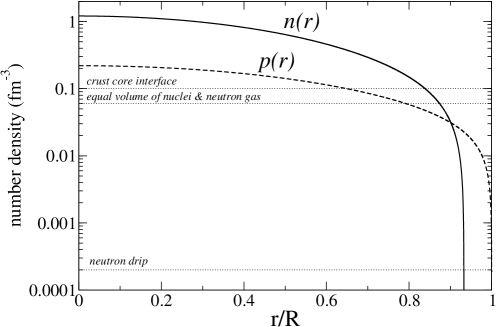
Figure 1: The radial profiles of the neutron and proton background particle number densities, $n$ and $p$, respectively, for model II. The model has been constructed such that it accords well with a $1.4M_{\odot}$ neutron star determined using the modern equation of state calculated by Akmal, Pandharipande and Ravenhall APR . For reference, we show as horizontal lines the number densities at which Akmal et al suggest that i) neutron drip occurs, ii) there is an equal number of nuclei and neutron gas, and iii) the crust/core interface is located. It should be noted that the latter should not coincide with our core/envelope interface since one would expect there to be a region where crust nuclei are penetrated by a neutron superfluid.

IV.2 Quasinormal modes

We have calculated the relevant fluid QNMs for our two stellar models, and various values of the entrainment parameter $\epsilon$. To put the results in context, it is useful to recall the basic features of the mode spectrum of a non-rotating, ordinary fluid neutron star. Despite the ordinary fluid system being the simplest possible description of the matter in a neutron star, there is nevertheless an impressive array of modes. In addition to the expected f- and p-modes, which are acoustic in nature, there also exists the so-called w-modes KS92 which are primarily due to oscillations of spacetime itself, with little coupling to the fluid of the star. If the equation of state has more than one parameter, and can be considered stratified — for instance, because of a varying proton fraction — then the star can also support low-frequency g-modes RG92 .

One might expect that the essential doubling of the matter degrees of freedom due to the presence of a superfluid component might simply lead to a doubling of the families of modes of oscillation. However, it should not come as a great surprise that the w-modes in a superfluid neutron star look very much like those of the ordinary fluid case CLL99 . There is no doubling of modes: The w-modes are a feature of spacetime itself and depend on the curvature induced by the background fluid rather than the actual nature of the fluid. But it is perhaps surprising that the simple expectation of mode doubling is not completely realized for the modes that are mainly due to matter oscillations. As mentioned in the Introduction, it has long been known that the additional fluid degree of freedom leads to the presence of a new set of modes, that have been dubbed superfluid modes. They are analogous to the ordinary fluid p-modes in that they are predominately acoustic in nature, (cf. Eq. (1)). The situation regarding g-modes is more confusing. Not only are there no new set of pulsating g-modes due to superfluidity, the standard set that one might expect to exist because of the varying proton fraction do not exist either. Inspired by Lee’s L95 numerical results, Andersson and Comer AC01a have used a local analysis of the mode spectrum to show that the g-modes disappear from the spectrum of pulsating modes. They prove that the “missing” g-modes exist as two independent sets of degenerate modes in the space of time-independent perturbations (the zero-frequency subspace). Their degeneracy will presumably be broken if one were to consider a two-fluid system governed by a three parameter equation of state. We plan to discuss this issue in detail elsewhere.

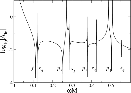
Figure 2: This figure shows the asymptotic amplitude $A_{\rm in}$ as a function of the (real) frequency $\omega M$ for our model I. The slowly-damped QNMs of the star show up as zeros of $A_{\rm in}$, i.e. deep minima in the figure. The first few “ordinary” and “superfluid” modes are identified in the figure, cf. Table III.

Since the w-modes are largely unaffected by superfluidity, and we do not expect pulsating g-modes, we focus our discussion on the ordinary fluid f- and p-modes as well as the superfluid s-modes. We mentioned in the Introduction that there are two characteristics that distinguish the s-modes from their ordinary fluid counterparts: (i) counter-motion of the neutrons with respect to the protons, and (ii) a strong dependence on the parameters of entrainment. We will leave until the next subsection the discussion on the effects of entrainment. Hence, we first consider the spectrum of fluid modes for a model with ${\cal A}=0$. In Fig. 2 we provide a graph of the incoming wave amplitude (see Appendix III) versus the real part of the mode frequency for our superfluid model I. As discussed in detail in Appendix III, a QNM corresponds to those particular solutions where there is no incoming wave at infinity. Hence, the QNM frequencies correspond to the deep minima that can be seen in Fig. 2. The main feature to notice is the presence of twice as many slowly damped fluid modes as in the ordinary fluid case, cf. Fig. 6 of CLL99 .

Table 2: The oscillation frequency and the associated damping rate (in terms of the real and imaginary parts of $\omega M$) for the first few fluid pulsation modes of model I. The w-modes for this model can be found in Table III of CLL99 .

mode	$f$	$s_{0}$	$p_{1}$	$s_{1}$	$p_{2}$	$s_{2}$
Re $\omega M$	0.137	0.157	0.306	0.354	0.585	0.688
Im $\omega M$	$7.2\times 10^{-5}$	$4.2\times 10^{-7}$	$6.6\times 10^{-6}$	$5.2\times 10^{-6}$	$3.2\times 10^{-7}$	$5.5\times 10^{-8}$

In the earlier work of Comer, Langlois, and Lin CLL99 , there was no attempt at determining the gravitational-wave damping times for either the ordinary fluid or the superfluid modes. The reason for this was the difficulty in determining complex QNM frequencies with imaginary parts that are orders of magnitude smaller than the real parts. To deal with this problem, we have developed a new method, which is outlined in Appendix III. The results we have obtained for model I are given in Table 2. As one can see, the ordinary fluid modes have damping rates that are consistent with what is known from calculations of ordinary fluid neutron stars LD ; DL . It should also be noticed that most of the superfluid modes have gravitational-wave damping rates that are similar to the high order p-modes. This is to be contrasted with recent statements in Ref. SW00 that superfluid modes will not radiate gravitationally. In fact, in Section V below we will provide a proof that all QNMs of a superfluid star must radiate. This means that the superfluid modes could, at least in principle, be relevant for gravitational-wave asteroseismology. This possibility will be discussed further in Section VI.

So far we have mainly discussed the results obtained for model I, for which there is no envelope. When we turn to model II, which has an ordinary fluid envelope of roughly one km, we find that the results do not change qualitatively. In particular, we do not find that new modes arise because of the presence of the envelope. At first this may seem a little bit surprising. Especially since it is well known that an elastic crust supports several additional sets of modes. However, in our case the absence of new modes is due to the nature of the phase transition at the core/envelope interface. We have chosen the phase-transition to be second order, which means that the number density of the protons remains smooth as the superfluid neutron component vanishes (at $r\to R_{c}$). Should we have taken the phase-transition to be first order, i.e. allowed for a jump in the proton number density at $R_{c}$, our calculations would have unveiled a set of interface g-modes.

IV.3 The effect of entrainment — avoided mode crossings

The two main goals of the work presented in this paper were: i) to allow for the presence of a core/envelope transition, and thus in principle be able to consider cases where the superfluid constituent is confined only to a part of the star, and ii) to determine how entrainment affects the QNM frequencies. As we will now discuss, the effect of entrainment can be considerable.

We have carried out a series of calculations for model II and entrainment parameters in the “physical range” $0.04<\epsilon<0.2$. A sample of results are given in Table 3. Listed there are the oscillation frequencies and associated damping rates for the first few pulsation modes of model II and three different values of $\epsilon$. First of all it is relevant to compare the results for the case of vanishing entrainment to those for model I, cf. Table 2. Recall that the main difference between models I and II is that the latter includes an ordinary fluid envelope. Nevertheless, it is clear from the numerical results that the QNMs of the two models are qualitatively quite similar. When we turn to the effect of varying the entrainment parameter we find that the superfluid mode frequencies shift considerable, while the ordinary fluid modes remain virtually unchanged. This is not a surprising result given the discussion in Ref. AC01a and Eq. (1). It is also relevant to note that the gravitational-wave damping rates can be strongly affected by a change in $\epsilon$.

Table 3: The oscillation frequency and the associated damping rate (in terms of the real and imaginary parts of $\omega M$) for the first few fluid pulsation modes of model II. We show results for three different values of the entrainment parameter $\epsilon$. These correspond to the case of no entrainment as well as the upper and lower limits for the range that we take as “physically realistic”. From this data we see that, while the ordinary fluid modes are hardly at all affected by the entrainment, the superfluid mode frequencies vary by as much as 10% as $\epsilon$ is varied within the realistic range.

	mode	$f$	$s_{0}$	$p_{1}$	$s_{1}$	$p_{2}$	$s_{2}$	$p_{3}$	$s_{3}$
$\epsilon=0$	Re $\omega M$	0.112	0.124	0.252	0.288	0.379	0.424	0.502	0.554
	Im $\omega M$	$4.9\times 10^{-5}$	$8.9\times 10^{-6}$	$1.3\times 10^{-5}$	$1.4\times 10^{-5}$	$8.0\times 10^{-8}$	$1.3\times 10^{-7}$	$1.5\times 10^{-8}$	$1.7\times 10^{-9}$
$\epsilon=0.04$	Re $\omega M$	0.113	0.130	0.253	0.299	0.382	0.442	0.507	0.577
	Im $\omega M$	$5.3\times 10^{-5}$	$5.3\times 10^{-6}$	$1.4\times 10^{-5}$	$8.5\times 10^{-7}$	$9.2\times 10^{-8}$	$1.2\times 10^{-7}$	$1.2\times 10^{-8}$	$4.3\times 10^{-9}$
$\epsilon=0.2$	Re $\omega M$	0.113	0.149	0.257	0.328	0.394	0.491	0.523	0.639
	Im $\omega M$	$5.5\times 10^{-5}$	$3.2\times 10^{-6}$	$1.4\times 10^{-5}$	$3.2\times 10^{-7}$	$1.0\times 10^{-7}$	$1.2\times 10^{-7}$	$2.3\times 10^{-9}$	$1.2\times 10^{-8}$

As we will now discuss, the effect that a varying entrainment has on the damping rate of the modes can be understood from the results illustrated in Figs. 3 and 4. Fig. 3 shows how the oscillation frequencies for the first few modes change as the entrainment parameter is varied within the acceptable range. The modes that have ordinary fluid behavior, i.e. for which the neutrons and protons “flow together”, in the limit of vanishing entrainment are shown as solid lines in the figure whereas the superfluid modes, where the neutrons and protons are largely counter-moving, are given by the dashed lines. The main feature of the figure is the presence of so-called avoided crossings. For the higher order modes (near the top of the figure) there are points in the $(\epsilon,{\rm Re}~{}\omega M)$ plane where the solid and dashed lines approach each other, but rather than crossing they diverge from each other. An interesting aspect of these avoided crossings can be gleaned from Fig. 4, which shows the Lagrangian variations $\Delta n$ and $\Delta p$ for the particular modes that correspond to the points $a_{\epsilon}$ and $b_{\epsilon}$, $\epsilon=0,0.1,0.2$, of Fig. 3. For the mode $a$ the two fluids are largely counter-moving as $\epsilon\to 0$, and for mode $b$ the two fluids are then comoving. However, as $\epsilon\to 0.2$ we see that the modes have changed character in that it is now mode $a$ that is comoving and mode $b$ that is counter-moving. This exchange of character of modes is a characteristic of avoided crossings familiar from other problems in stellar pulsation theory japan . The presence of avoided crossings between stellar pulsation modes is familiar from many other situations, but we believe that our results provide the first hard evidence for the presence of this phenomenon in superfluid stars.

From general post-Newtonian arguments, one would expect the co-moving modes to radiate gravitational waves more efficiently than the counter-moving superfluid modes. Thus it is not surprising to find that the damping rate of a superfluid mode increases as entrainment is varied and an avoided crossing is approached. In the present context, this effect is probably not distinct enough to be of great relevance but one can argue that it may be of great importance in closely related problems. As has been argued recently AC01a , avoided crossings may be at the heart of recent calculations of the effect of superfluidity on the r-mode instability. Lindblom and Mendell LM00 have analyzed the effect of mutual friction damping on the r-modes using the same entrainment model as we employ here. They found that mutual friction was, in general, not effective at damping the r-modes. However, they also found (cf. their Fig. 6) that the mutual friction damping time could be very small for particular values of $\epsilon$. We believe that a proper explanation of this result can be obtained via the avoided crossings phenomenon. The basic idea is that mutual friction should be most effective whenever the neutrons and protons are counter-moving, as with the superfluid modes. Andersson and Comer AC01a have shown that there are two sets of r-modes, that are quite analogous to the ordinary fluid and superfluid modes discussed in this paper in the sense that one set has the neutrons and protons comoving whereas the other set has them countermoving. Although avoided crossings between these two classes of r-modes in a superfluid star have not yet been demonstrated, we believe that our current results provide strong support for the idea by demonstrating the presence of avoided crossings in a very closely connected situation. We thus assert that the particular values of $\epsilon$ for with Lindblom and Mendell find small mutual friction damping times correspond to stellar models for which the two classes of superfluid r-modes are close to an avoided crossing. The veracity of this argument remains to be confirmed by detailed calculations that we plan to carry out in the near future.

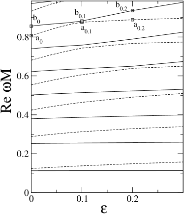
Figure 3: This figure shows how the frequencies of the fluid pulsation modes for our model II vary with the entrainment parameter $\epsilon$. The modes shown as solid lines are such that the two fluids are essentially comoving in the $\epsilon\to 0$ limit, while the modes shown as dashed lines are countermoving. As is apparent from the data, the higher order modes exhibit avoided crossings as $\epsilon$ varies. Recall that the range often taken as “physically relevant” is $0.04\leq\epsilon\leq 0.2$. We indicate by $a_{\epsilon}$ and $b_{\epsilon}$ the particular modes for which the eigenfunctions are shown in Fig. 4.

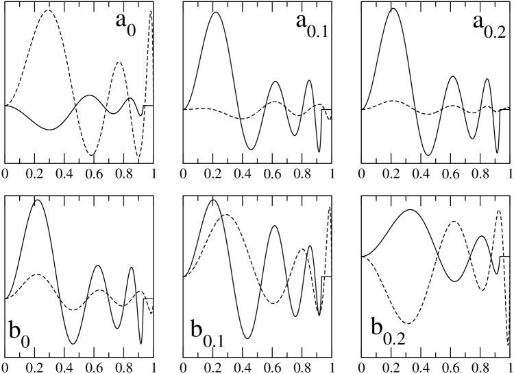
Figure 4: An illustration of the fact that the modes exchange properties during an avoided crossing. We consider two modes, labelled by $a_{\epsilon}$ and $b_{\epsilon}$ (cf. Figure 3). The mode eigenfunctions are represented by the two Lagrangian number density variations, $\Delta n$ and $\Delta p$ (solid and dashed lines, respectively). For mode $a$ the two fluids are essentially countermoving in the $\epsilon\to 0$ limit (it is a superfluid mode), while the two fluids comove for mode $b$ (it is similar to a standard p-mode). After the avoided crossing (which takes place roughly at $\epsilon=0.1$) the two modes have exchanged properties.

V Are there non-radiative modes in superfluid neutron stars?

In this Section we digress somewhat and focus our attention on a question of principle: Is it possible to have QNMs that do not radiate gravitationally in a superfluid star? The question is motivated by the simple fact that, while every non-radial motion induced in a one-fluid system must lead to the emission of gravitational waves, the situation could conceivably be different in the two-fluid case. One can imagine the possibility that the two fluids move in such a way that the average mass-density flux vanishes identically. In fact, as we have discussed elsewhere AC01a , the superfluid modes are essentially of this nature and it has been argued by Sedrakian and Wasserman SW00 that this means that these modes will not radiate. Of course, one must not forget that, in the post-Newtonian picture, gravitational waves are associated with both mass- and current multipoles. Thus even the extreme case of a two-fluid oscillation such that the mass-multipoles vanish identically is likely to radiate through the induced currents. Thus it may be very difficult to set the two fluids into motion without generating gravitational waves. And this is, indeed, the way that it turns out. As we will prove below, a two-fluid star can (in general) have no non-radiative modes.

We consider the superfluid perturbation equation in the special case where the metric is left completely unperturbed, i.e. when no gravitational radiation is created. Assuming a given, fixed non-rotating background, we can obtain the corresponding field equations by setting to zero the three metric perturbation $H_{0}$, $H_{1}$, and $K$. This results in the following nine equations for six matter variables, cf. Eqns (34)-(59),

$$0 = {X_{n}}+{X_{p}}\ ,$$ (105)

$$0 = \mu n{V_{n}}+\chi p{V_{p}}\ ,$$ (107)

$$0 = \mu n{W_{n}}+\chi p{W_{p}}\ ,$$ (109)

$${W_{n}}^{\prime} = -e^{\lambda/2}{l(l+1)\over r}{V_{n}}-\left({l+1\over r}+{n^{\prime}\over n}\right){W_{n}}$$ (113)

$$+{{{\cal C}_{0}^{0}}\over n^{2}{{\cal D}_{0}^{0}}}\left[e^{(\lambda-\nu)/2}r{X_{n}}+n^{\prime}\left({{\cal B}_{0}^{0}}n{W_{n}}+{{\cal A}_{0}^{0}}p{W_{p}}\right)\right]-$$

$${{{\cal A}_{0}^{0}}\over np{{\cal D}_{0}^{0}}}\left[e^{(\lambda-\nu)/2}r{X_{p}}+p^{\prime}\left({{\cal A}_{0}^{0}}n{W_{n}}+{{\cal C}_{0}^{0}}p{W_{p}}\right)\right]\ ,$$

$${W_{p}}^{\prime} = -e^{\lambda/2}{l(l+1)\over r}{V_{p}}-\left({l+1\over r}+{p^{\prime}\over p}\right){W_{p}}$$ (117)

$$+{{{\cal B}_{0}^{0}}\over p^{2}{{\cal D}_{0}^{0}}}\left[e^{(\lambda-\nu)/2}r{X_{p}}+p^{\prime}\left({{\cal C}_{0}^{0}}p{W_{p}}+{{\cal A}_{0}^{0}}n{W_{n}}\right)\right]-$$

$${{{\cal A}_{0}^{0}}\over np{{\cal D}_{0}^{0}}}\left[e^{(\lambda-\nu)/2}r{X_{n}}+n^{\prime}\left({{\cal A}_{0}^{0}}p{W_{p}}+{{\cal B}_{0}^{0}}n{W_{n}}\right)\right]\ ,$$

$${X_{n}}^{\prime} = -{l\over r}{X_{n}}+{l(l+1)\over r^{2}}e^{\nu/2}n^{\prime}\left({{\cal B}_{0}^{0}}n{V_{n}}+{{\cal A}_{0}^{0}}p{V_{p}}\right)$$ (122)

$$-e^{(\lambda-\nu)/2}{\omega^{2}\over r}n\left({\cal B}n{W_{n}}+{\cal A}p{W_{p}}\right)$$

$$+e^{-(\lambda-\nu)/2}\left[-{n^{\prime}\over r}\left({{\cal B}_{0}^{0}}^{\prime}n{W_{n}}+{{\cal A}_{0}^{0}}^{\prime}p{W_{p}}\right)+\right.$$

$$\left.\left({2n^{\prime}\over r^{2}}+{\lambda^{\prime}-\nu^{\prime}\over 2r}n^{\prime}-{n^{\prime\prime}\over r}\right)\left({{\cal B}_{0}^{0}}n{W_{n}}+{{\cal A}_{0}^{0}}p{W_{p}}\right)\right]\ ,$$

$${X_{p}}^{\prime} = -{l\over r}{X_{p}}+{l(l+1)\over r^{2}}e^{\nu/2}p^{\prime}\left({{\cal C}_{0}^{0}}p{V_{p}}+{{\cal A}_{0}^{0}}n{V_{n}}\right)$$ (127)

$$-e^{(\lambda-\nu)/2}{\omega^{2}\over r}p\left({\cal C}p{W_{p}}+{\cal A}n{W_{n}}\right)$$

$$+e^{-(\lambda-\nu)/2}\left[-{p^{\prime}\over r}\left({{\cal C}_{0}^{0}}^{\prime}p{W_{p}}+{{\cal A}_{0}^{0}}^{\prime}n{W_{n}}\right)+\right.$$

$$\left.\left({2p^{\prime}\over r^{2}}+{\lambda^{\prime}-\nu^{\prime}\over 2r}p^{\prime}-{p^{\prime\prime}\over r}\right)\left({{\cal C}_{0}^{0}}p{W_{p}}+{{\cal A}_{0}^{0}}n{W_{n}}\right)\right]\ ,$$

with

$${X_{n}}\equiv ne^{-\nu/2}\omega^{2}\left({\cal B}n{V_{n}}+{\cal A}p{V_{p}}\right)-e^{(\nu-\lambda)/2}{n^{\prime}\over r}\left({{\cal B}_{0}^{0}}n{W_{n}}+{{\cal A}_{0}^{0}}p{W_{p}}\right)\ ,$$ (128)

and

$${X_{p}}\equiv pe^{-\nu/2}\omega^{2}\left({\cal C}p{V_{p}}+{\cal A}n{V_{n}}\right)-e^{(\nu-\lambda)/2}{p^{\prime}\over r}\left({{\cal C}_{0}^{0}}p{W_{p}}+{{\cal A}_{0}^{0}}n{W_{n}}\right)\ .$$ (129)

It is clear that, unless some of these equations are linearly dependent the problem is overdetermined and we cannot have a non-trivial solution. In order to show that the problem is in general overdetermined, we use the first three equations above to rewrite $W_{p}$, $V_{p}$, and $X_{p}$ in terms of the neutron variables $W_{n}$, $V_{n}$, and $X_{n}$, and then substitute these into the remaining six equations. Remarkably, one finds that Eqs. (122) and (127) yield exactly the same result when this substitution is done. One also finds that Eqs. (30) and (31) yield the same result after the substitution. We are thus left with Eqs. (113) and (117). After the substitution, these equations yield the following two equations for $W_{n}$:

$$W^{\prime}_{n} = -e^{\lambda/2}{l(l+1)\over r}V_{n}-{l+1\over r}W_{n}+{{{\cal A}_{0}^{0}}\over{{\cal D}_{0}^{0}}}\left({{\cal A}_{0}^{0}}-{\mu\over\chi}{{\cal C}_{0}^{0}}\right)\left({n^{\prime}\over n}-{p^{\prime}\over p}\right)W_{n}$$ (131)

$$+e^{(\lambda-\nu)/2}r\left({{{\cal C}_{0}^{0}}p+{{\cal A}_{0}^{0}}n\over pn^{2}{{\cal D}_{0}^{0}}}\right)X_{n}\ ,$$

$$W^{\prime}_{n} = -e^{\lambda/2}{l(l+1)\over r}V_{n}-{l+1\over r}W_{n}-{{{\cal B}_{0}^{0}}\over{{\cal D}_{0}^{0}}}\left({{\cal C}_{0}^{0}}-{\chi\over\mu}{{\cal A}_{0}^{0}}\right)\left({n^{\prime}\over n}-{p^{\prime}\over p}\right)W_{n}$$ (134)

$$+e^{(\lambda-\nu)/2}r{\chi\over\mu}\left({{{\cal B}_{0}^{0}}n+{{\cal A}_{0}^{0}}p\over pn^{2}{{\cal D}_{0}^{0}}}\right)X_{n}\ .$$

In the manipulations we have used repeatedly the background equations (11) and

$$\mu^{\prime}=-{1\over 2}\mu\nu^{\prime}\quad,\quad\chi^{\prime}=-{1\over 2}\chi\nu^{\prime}\ .$$ (135)

In order to complete the argument in a clear way, we restrict ourselves to the case of vanishing entrainment and separable equations of state, i.e. we concentrate on the case ${\cal A}={{\cal A}_{0}^{0}}=0$. This is not at all necessary, but it simplifies the analysis considerably since the involved relations are much simpler. Taking the difference between (131) and (134) we require

$${\cal B}_{0}^{0}{\cal C}_{0}^{0}\left({n^{\prime}\over n}-{p^{\prime}\over p}\right)W_{n}+{e^{(\lambda-\nu)/2}r\over pn^{2}}\left({\cal C}_{0}^{0}p-{\chi\over\mu}{\cal B}_{0}^{0}n\right)X_{n}=0$$ (136)

in order for the problem not to be over-determined. Using the definition of $X_{n}$ we can rewrite this equation as

$$e^{\lambda/2-\nu}r\omega^{2}{\cal B}\left({\cal C}_{0}^{0}-{n\chi\over p\mu}{\cal B}_{0}^{0}\right)V_{n}+{{\cal B}_{0}^{0}\over p}\left(n^{\prime}{\cal B}_{0}^{0}{\chi\over\mu}-p^{\prime}{\cal C}_{0}^{0}\right)W_{n}=0\ .$$ (137)

Now using the fact that $\chi\equiv{\cal C}p$ and $\mu\equiv{\cal B}n$ in the case of vanishing entrainment, we have

$$e^{\lambda/2-\nu}r\omega^{2}\left({\cal B}{\cal C}_{0}^{0}-{\cal C}{\cal B}_{0}^{0}\right)V_{n}+{{\cal B}_{0}^{0}\over{\cal B}}\left({\cal C}{\cal B}_{0}^{0}{n^{\prime}\over n}-{\cal B}{\cal C}_{0}^{0}{p^{\prime}\over p}\right)W_{n}=e^{\lambda/2-\nu}r\omega^{2}\left({\cal B}{\cal C}_{0}^{0}-{\cal C}{\cal B}_{0}^{0}\right)V_{n}=0\ .$$ (138)

To arrive at the last equality we have employed the background identities (11) again. Clearly, we are now left with two possibilities. Either $V_{n}$ vanishes, or the equation of state must be such that

$${\cal B}{\cal C}_{0}^{0}-{\cal C}{\cal B}_{0}^{0}=0\ .$$ (139)

In the first case one can show that the corresponding solution for $W_{n}$ is

$$W_{n}\propto{1\over nr^{l+1}}\ .$$ (140)

This solution is clearly physically unacceptable since it diverges at the centre of the star. In other words, if $V_{n}=0$ we must also have $W_{n}=0$, i.e. the trivial solution. It is easy to show that the second case requires that the master function be such that

$$8p^{2}{\partial\Lambda\over\partial n^{2}}{\partial\over\partial p^{2}}\left({\partial\Lambda\over\partial p^{2}}\right)-8n^{2}{\partial\Lambda\over\partial p^{2}}{\partial\over\partial n^{2}}\left({\partial\Lambda\over\partial n^{2}}\right)=0\ .$$ (141)

This is clearly a very particular form. We have thus proven that the QNMs of a superfluid star must radiate unless the equation of state belongs to a very special class. The obvious exceptions are i) when the master function takes the form

$$\Lambda=\sigma_{n}n^{2}+\sigma_{p}p^{2}$$ (142)

and ii) whenever $\Lambda$ depends on $n$ and $p$ in identical ways.

It is worth pointing out that the calculation in this section was carried out within the Regge-Wheeler gauge, and given possible gauge issues one may worry that this means that the result is of limited validity. However, the result will hold in general since we can easily construct gauge-invariant quantities (such as the Zerilli function) that represent the gravitational-wave degrees of freedom from the metric perturbations calculated in any particular gauge. In our case it is trivial to see that, if all metric perturbations vanish identically the Zerilli function will be identically zero and no gravitational-waves will emerge from the system.

VI Detectable Gravitational Wave Signals?

Given that a new generation of gravitational-wave detectors are likely to be operating at their projected levels sensitivity within the next few months, it is appropriate to conclude this paper with a brief discussion of a possible future application of our results. Suppose that the various modes of a superfluid neutron star were excited to an amplitude such that the associated gravitational-wave signal could be detected. To what extent would it then be possible to solve the inverse problem and deduce information concerning the superfluid parameters? In other words, can we hope to use “gravitational-wave asteroseismology” to probe the superfluid interior of mature neutron stars? This question has recently been discussed by two of us AC01b , and therefore we only provide a brief background here.

As has already been discussed by Kokkotas et al astero2 , the detection of gravitational-wave signals from pulsations in newly born neutron stars could be used to infer the mass and radius of the star. This information would put strong constraints on the supranuclear equation of state. However, this argument relies on releasing an energy equivalent to something like $10^{-5}M_{\odot}c^{2}$ through the QNMs. This may not be unreasonable for the wildly pulsating object formed through a strongly asymmetric supernova collapse, but it is difficult to think of a mechanism whereby the oscillations of a mature (and thus superfluid) neutron star core will be excited to a similar level. Instead, we take as a “reasonable” order of magnitude estimate the energy associated with a typical pulsar glitch. The released energy can then be estimated as

$$\Delta E\approx I\Omega\Delta\Omega\approx(10^{-6}-10^{-8})I\Omega^{2}$$ (143)

where $\Omega=2\pi/P$ is the rotation rate of the star, and $P$ is the observed pulsar period. In this formula it is appropriate to use the moment of inertia $I\sim 10^{45}$ gcm² of the entire star, since the spin-up incurred during the glitch remains on timescales that are much longer than the estimated coupling timescale between the crust and the core fluid. By combining the above formula with the data for typical glitches in the Crab and Vela pulsars, cf. Table 4, we arrive at estimates of the energy associated with typical glitches that accord well with suggestions in the literature franco00 ; hart00 .

Table 4: Data for archetypal glitching pulsars.

PSR	$P$ (ms)	$d$ (kpc)	$\Delta\Omega/\Omega$	$\Delta E/M_{\odot}c^{2}$
Crab	33	2	$10^{-8}$	$2\times 10^{-13}$
Vela	89	0.5	$10^{-6}$	$3\times 10^{-12}$

As is evident from Table 4, we expect a glitch to be associated with energies of the order of $10^{-13}-10^{-12}M_{\odot}c^{2}$. In the following we will assume that a similar energy is channeled through the various pulsation modes. This then allows us to use the formulas obtained by Kokkotas et al astero2 to estimate, for a given detector configuration, the attainable signal-to-noise ratio.

Assume that the gravitational-wave signal from a neutron star pulsation mode takes the form of a damped sinusoidal, i.e.

$$h(t)={\cal A}e^{-(t-T)/t_{d}}\sin[2\pi f(t-T)]\quad\mbox{ for }t>T$$ (144)

where $f$ is the frequency of the QNM, $t_{d}$ is its characteristic damping time, and $T$ is the arrival time of the signal at the detector (thus $h(t)=0$ for $t<T$). Using standard results for the gravitational-wave flux astero2 , the amplitude ${\cal A}$ of the signal can be expressed in terms of the total energy radiated through the mode:

$${\cal A}\approx 7.6\times 10^{-24}\sqrt{{\Delta E_{\odot}\over 10^{-12}}{1\mbox{ s}\over t_{d}}}\left({1\mbox{ kpc}\over d}\right)\left({1\mbox{ kHz}\over f}\right)\ .$$ (145)

where $\Delta E_{\odot}=\Delta E/M_{\odot}c^{2}$. The signal-to-noise ratio for this signal can be estimated from astero2

$$\left({S\over N}\right)^{2}={4Q^{2}\over 1+4Q^{2}}{{\cal A}^{2}t_{d}\over 2S_{n}}$$ (146)

where the “quality factor” is $Q=\pi ft_{d}$ and $S_{n}$ is the spectral noise density of the detector.

We can now combine these estimates with the QNMs from (say) Table 2. The relevant frequencies and damping times in kHz and ms, respectively, are given in Table 5. When we compare the obtained estimates to the new generation of large-scale interferometric detectors it immediately becomes clear that these signals would be too weak to be detected. This is illustrated in Figure 5 where we compare the dimensionless strain $\sqrt{f}S_{n}$ for various detector configurations to the estimated strain caused by the QNM signals.

Table 5: The frequency and damping rate for the first few modes of our Model I (which is identical to model 2 of Comer et al CLL99 ). We also show the gravitational-wave signal-to-noise ratios resulting from the “glitch model” discussed in the main text. The results correspond to an advanced EURO detector with (case 1) and without (case 2) photon shotnoise, respectively. The lower estimate is for a Crab glitch while the upper estimate follows from the Vela data.

Mode	$f$ (kHz)	$t_{d}$ (s)	Case 1	Case 2
$f$	3.29	0.092	0.4—6	300—$4.7\times 10^{3}$
$p_{1}$	7.34	1.01	0.08—1.2	680—$1\times 10^{4}$
$s_{0}$	3.76	15.75	0.3—4.8	350—$5.4\times 10^{3}$
$s_{1}$	8.49	1.29	0.06—0.9	780—$1.2\times 10^{4}$

This does not, however, mean that we should give up on the main idea behind this analysis. We simply have to acknowledge that we are likely to require significant improvements in technology if we are to be able to make this into a viable approach. But it seems inevitable that the available technology will improve over the next decades. In fact, various groups are already discussing possible improvements in detector sensitivity that may be achievable in the future. In order to illustrate the levels that are being discussed, we consider the so-called EURO detector, for which the sensitivity has been estimated by Sathyaprakash and Schutz (for further details see euro ). We consider two possible configurations: In the first, the sensitivity at high frequencies is limited by the photon shot-noise, while the second configuration reaches beyond this limit by running several narrowbanded (cryogenic) interferometers as a “xylophone”. The corresponding noise-curves are illustrated, and compared to the current generation of interferometers, in Figure 5. It is immediately clear from Figure 5 that a EURO detector would be a superb instrument for studying pulsating neutron stars. This means that previously suggested strategies astero2 for unveiling the supranuclear equation of state may eventually be put to the test. In fact, as is clear from the estimates in Table 5, where we list the signal-to-noise ratio estimated from (146), one should also be able to detect the superfluid oscillation modes. The various modes would be marginally detectable given this level of excitation and a third generation detector limited by the photon shotnoise. If this limit can be surpassed by configuring several narrowbanded interferometers as a xylophone, the achievable signal-to-noise ratio will be excellent. Hence, it seems plausible that one could infer the parameters of neutron star superfluidity. As an obvious “by product” one might hope to shed light on the mechanism for pulsar glitches.

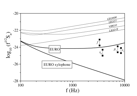
Figure 5: The spectral noise density for the new generation of laser-interferometric gravitational-wave detectors that will come online in the next few years (thin lines) is compared to speculative estimates for the futuristic EURO detector (solid lines). A key feature of this advanced configuration is that it may operate several narrowbanded interferometers as a xylophone, thus reaching high sensitivity at kHz frequencies. We also indicate the effective gravitational-wave amplitudes from the glitch-induced mode-oscillations discussed in the text.

We can also confirm that, provided that the modes can be detected, the oscillation frequencies can be extracted with good accuracy from the data. By combining Eqns. (11) and (12) from Kokkotas et al astero2 with (146) one can obtain a formula for the signal-to-noise required to determine the mode frequency with a relative error $\sigma_{f}/f$. We get (since $Q>>1$ for the modes under consideration) a relation

$$\left({S\over N}\right)\approx 0.33\left({1\mbox{ s}\over t_{d}}\right)\left({\mbox{1 kHz}\over f}\right)\left({\sigma_{f}\over f}\right)^{-1}$$ (147)

From this relation we can deduce that a detection with signal-to-noise of (say) 10 would enable one to infer the fluid mode frequencies with an accuracy of the order of a percent or so. With this level of precision one should be able to distinguish clearly between the “normal fluid” f and p-modes and the superfluid s-modes. In other words, we would have the information required not only to infer the mass and radius of the star astero2 , we could also hope to constrain the parameters of neutron star superfluidity.

VII Conclusions

The main motivation behind the work presented in this paper is the fact that neutron star physics is not adequately modelled within Newtonian gravity. It is well known that Newtonian results differ greatly from the correct relativistic ones already at the level of determining the mass and radius of a star with a prescribed central density from a given “realistic” equation of state. As far as the QNMs of the star are concerned, Newtonian studies are extremely useful since they help us understand the physics of different classes of modes. But at the same time it is clear that if we require a detailed model of the oscillation spectrum of an astrophysical neutron star we must approach the problem from the relativistic point of view. This is particularly crucial if we are interested in the gravitational-wave damping rates. Furthermore, since mature neutron stars are likely to contain several superfluid components, it is important that we develop a framework for modelling multi-fluid systems in full general relativity. The present paper represents significant progress towards this goal.

We have considered a core-envelope model, with superfluid neutrons being present only in the core of the star while the outer region is composed of an ordinary fluid. Our model includes a simple, yet reasonable, model for entrainment and we have shown how neighbouring QNMs undergo avoided crossings as the entrainment parameter is varied. Finally, we have ruled out the possibility that a two-fluid star could have non-radiative pulsation modes, and discussed the possible detection of gravitational-wave signals from oscillating superfluid neutron stars.

In the near future, our aim is to turn our attention to the oscillations of rotating superfluid stars. This is an exciting problem area, since various modes of oscillation may be driven unstable by the emission of gravitational waves. Of particular recent interest are the so-called r-modes, and the damping due to superfluid mutual friction. In a recent work, Lindblom and Mendell LM00 showed that mutual friction was effective at damping unstable r-modes only for very particular values of the entrainment parameter. Andersson and Comer AC01a have speculated that this peculiar behavior might be due to the existence of avoided crossings between two classes of r-modes (analogous to the two classes of acoustic fluid modes discussed in the present paper). The results of the present paper lend support to this idea. Yet it is clear that our understanding of the various involved issues is far from complete, and that a considerable amount of work remains to be done before we can model the dynamics of rotating superfluid neutron stars in a “realistic” way.

Appendix I: The Junction Conditions

In this Appendix will be presented a geometrical approach to deriving the junction conditions that must be used to smoothly join together an inner superfluid core with an exterior normal fluid envelope. The junction conditions will be obtained via an analysis of the first and second fundamental forms associated with the (in general, timelike) hypersurfaces given by the level surfaces of the generalized pressure $\Psi$ (cf. Eq. (3)) . If there are no “delta-function-like” discontinuities in the pressure, then the first and second fundamental forms will be continuous throughout the star MTW . Turning the problem around, by demanding the continuity of the first and second fundamental forms a smooth joining at the core/envelope interface can be achieved.

Consider that the level surfaces of $\Psi$ are timelike, i.e. the normal to these surfaces is given by

$${\cal N}^{\mu}={g^{\mu\nu}\nabla_{\nu}\Psi\over\sqrt{\nabla_{\mu}\Psi\nabla^{\mu}\Psi}}\ ,$$ (148)

where ${\cal N}_{\mu}{\cal N}^{\mu}=1$. The so-called first fundamental form $\gamma_{\mu\nu}$ (i.e. the induced three-metric) of these level surfaces is

$$\gamma_{\mu\nu}=\perp^{\sigma}_{\mu}\perp^{\tau}_{\nu}g_{\sigma\tau}\ ,$$ (149)

where the “perp” operator $\perp^{\sigma}_{\mu}$ is given by

$$\perp^{\sigma}_{\mu}=\delta^{\sigma}_{\mu}-{\cal N}^{\sigma}{\cal N}_{\mu}\ .$$ (150)

The second fundamental form $K_{\mu\nu}$ (i.e. the extrinsic curvature) of the level surfaces is defined as

$$K_{\mu\nu}=-\perp^{\sigma}_{\mu}\perp^{\tau}_{\nu}\nabla_{(\sigma}{\cal N}_{\tau)}\ ,$$ (151)

where the parentheses imply symmetrization of the indices.

Let us consider the pressure to be of form

$$\Psi(t,r,\theta)=\Psi_{0}(r)+\delta\Psi(t,r,\theta)\ .$$ (152)

The components of the unit normal ${\cal N}^{\mu}$ are thus found to be

$${\cal N}^{0} = -e^{\lambda/2-\nu}{\delta\dot{\Psi}\over\Psi_{0}^{\prime}}+e^{-(\lambda/2+\nu)}\delta g_{01}\ ,$$ (153)

$${\cal N}^{1} = e^{-\lambda/2}\left(1-\delta g_{11}/2e^{\lambda}\right)\ ,$$ (155)

$${\cal N}^{2} = {e^{\lambda/2}\over r^{2}}{\delta\Psi_{,\theta}\over\Psi_{0}^{\prime}}\ ,$$ (157)

$${\cal N}^{3} = 0\ .$$ (159)

The non-zero components of the first fundamental form are

$$\gamma_{00} = -e^{\nu}+\delta g_{00}\ ,\quad\gamma_{01}=\delta g_{01}-e^{\lambda}{\delta\dot{\Psi}\over\Psi_{0}^{\prime}}\ ,\quad\gamma_{12}=-e^{\lambda}{\delta\Psi_{,\theta}\over\Psi_{0}^{\prime}}\ ,$$ (160)

$$\gamma_{22} = r^{2}+\delta g_{22},\quad\gamma_{33}={\rm sin}^{2}\theta r^{2}+\delta g_{33}\ ,$$ (162)

and we also find

$$K_{00} = {\nu^{\prime}\over 2}e^{\nu-\lambda/2}-e^{\lambda/2}{\delta\ddot{\Psi}\over\Psi^{\prime}_{0}}+{1\over e^{\lambda/2}}\delta\dot{g}_{01}-{1\over 2e^{\lambda/2}}\delta g^{\prime}_{00}+{\nu^{\prime}\over 4}e^{\nu-3\lambda/2}\delta g_{11}\ ,$$ (163)

$$K_{01} = {\nu^{\prime}\over 2}\left(e^{\lambda/2}{\delta\dot{\Psi}\over\Psi_{0}^{\prime}}-e^{-\lambda/2}\delta g_{01}\right),\quad K_{02}=-e^{\lambda/2}\left({\delta\dot{\Psi}_{,\theta}\over\Psi_{0}^{\prime}}-{1\over 2e^{\lambda}}\delta g_{01,\theta}\right)\ ,$$ (165)

$$K_{12} = {e^{\lambda/2}\over r}{\delta\Psi_{,\theta}\over\Psi^{\prime}_{0}},\quad K_{22}=-{r\over e^{\lambda/2}}-e^{\lambda/2}{\delta\Psi_{,\theta\theta}\over\Psi^{\prime}_{0}}-{1\over 2e^{\lambda/2}}\left(\delta g^{\prime}_{22}-{r\over e^{\lambda}}\delta g_{11}\right)\ ,$$ (167)

$$K_{33} = -{\rm sin}^{2}\theta\left({r\over e^{\lambda/2}}+{\rm cot}\theta e^{\lambda/2}{\delta\Psi_{,\theta}\over\Psi^{\prime}_{0}}+{1\over 2{\rm sin}^{2}\theta e^{\lambda/2}}\delta g^{\prime}_{33}-{r\over 2e^{3\lambda/2}}\delta g_{11}\right)\ ,$$ (169)

for the non-trivial components of the second fundamental form.

Given that a smooth background can be constructed independently of the oscillations, we can assume that the background and linearized pieces of $\gamma_{\mu\nu}$ and $K_{\mu\nu}$ are separately continuous at the core-envelope interface. We will consider the background pieces first. For clarity of presentation the matter and metric variables in the envelope will be distinguished by a tilde. The continuity of the first fundamental form thus yields for the background

$$\nu(R_{c})=\tilde{\nu}(R_{c})\ ,$$ (170)

and continuity of the second fundamental form implies

$$\nu^{\prime}(R_{c})=\tilde{\nu}^{\prime}(R_{c})\quad,\quad e^{\lambda(R_{c})}=e^{\tilde{\lambda}(R_{c})}\ .$$ (171)

Using the background Einstein equations, and defining

$$e^{-\lambda}=1-2m(r)/r\quad,\quad e^{-\tilde{\lambda}}=1-2\tilde{m}(r)/r\ ,$$ (172)

where

$$m(r)=-4\pi\int_{0}^{r}r^{2}\Lambda_{0}(r)dr\quad,\quad\tilde{m}(r)=-4\pi\int_{R_{c}}^{r}r^{2}\tilde{\Lambda}_{0}(r)dr+C\ ,$$ (173)

we find that the background junction conditions imply $C=m(R_{c})$ and $\Psi_{0}(R_{c})=\tilde{\Psi}_{0}(R_{c})$, where $\tilde{\Psi}_{0}$ and $-\tilde{\Lambda}_{0}$ are the pressure and energy density of the envelope, respectively. It is also useful to note that the Tolman-Oppenheimer-Volkov equations for the core and envelope imply

$${\Psi^{\prime}_{0}(R_{c})\over\tilde{\Psi}^{\prime}_{0}(R_{c})}={\Psi_{0}(R_{c})-\Lambda_{0}(R_{c})\over\tilde{\Psi}_{0}(R_{c})-\tilde{\Lambda}_{0}(R_{c})}\ .$$ (174)

Before dealing with the linear perturbations, it will be convenient to write out the linearized pressure as a function of the fundamental matter and metric variables, for both the core and the envelope. We have used the field equations to help simplify the formulas. The final forms are (for the radial dependence)

$$\delta\Psi=\left[{\nu^{\prime}\over 2re^{\lambda/2}}\left(\mu nW_{n}+\chi pW_{p}\right)-{1\over e^{\nu/2}}\left(X_{n}+X_{p}\right)\right]r^{l}$$ (175)

and

$$\delta\tilde{\Psi}=\left[{\tilde{\nu}^{\prime}\over 2re^{\tilde{\lambda}/2}}\tilde{\chi}\tilde{p}\tilde{W}_{p}-{1\over e^{\tilde{\nu}/2}}\tilde{X}_{p}\right]r^{l}$$ (176)

where we have again put a tilde over all the linearized variables associated with the envelope. Now, it can be seen that the junction conditions imply that the metric perturbations are continuous at the core/envelope interface, i.e.

$$H_{0}(R_{c}) = \tilde{H}_{0}(R_{c})\ ,$$ (177)

$$H_{1}(R_{c}) = \tilde{H}_{1}(R_{c})\ ,$$ (179)

$$K(R_{c}) = \tilde{K}(R_{c})\ .$$ (181)

The matter variables, on the other hand, must satisfy two conditions, which are

$$\tilde{\chi}(R_{c})\tilde{p}(R_{c})\tilde{W}_{p}(R_{c})=\mu(R_{c})n(R_{c})W_{n}(R_{c})+\chi(R_{c})p(R_{c})W_{p}(R_{c})$$ (182)

and

$$\tilde{X}_{p}(R_{c}) = {\tilde{\Psi}_{0}(R_{c})-\tilde{\Lambda}_{0}(R_{c})\over\Psi_{0}(R_{I})-\Lambda_{0}(R_{c})}\left({X_{n}}(R_{c})+{X_{p}}(R_{c})\right)-{\nu^{\prime}(R_{c})e^{(\nu(R_{c})-\lambda(R_{c}))/2}\over 2R_{c}}\left({\tilde{\Psi}_{0}(R_{c})-\tilde{\Lambda}_{0}(R_{c})\over\Psi_{0}(R_{c})-\Lambda_{0}(R_{c})}-1\right)\times$$ (185)

$$\tilde{\chi}(R_{c})\tilde{p}(R_{c})\tilde{W}_{p}(R_{c})\ .$$

It is important to notice that the junction conditions do not imply that $\delta\Psi=\delta\tilde{\Psi}$ at the core/envelope interface, but rather that $\delta\Psi/\Psi_{0}^{\prime}=\delta\tilde{\Psi}/\tilde{\Psi}_{0}^{\prime}$. This fact is the clearest demonstration why a geometrical approach is crucial for obtaining the correct junction conditions, since this particular result is a direct consequence of the fact that Schwarzschild-like coordinates cause derivative discontinuities whenever the energy density is not continuous. If it is the case that $\Lambda_{0}(R_{c})=\tilde{\Lambda}_{0}(R_{c})$, then we can see from Eq. (174) that the junction conditions will imply $\delta\Psi=\delta\tilde{\Psi}$. Having a continuous energy density also implies that $\tilde{X}_{p}(R_{c})=X_{n}(R_{c})+X_{p}(R_{c})$.

Appendix II: The Analytical Equation of State

In this Appendix we develop the analytical equation of state used in the main part of the text. The essential strategy is to introduce an expansion based on the assumption that the fluid velocities are small compared to the speed of light. This is a reasonable assumption for neutron star pulsations.

VII.1 A Local Analysis of the Entrainment Parameter

Recall that the entrainment variable $x^{2}$ is given by $x^{2}=-n^{\mu}p_{\mu}$. It is convenient to write each conserved four-current as in the main text:

$$n^{\rho}=nu^{\rho}\quad,\quad p^{\rho}=pv^{\rho}\ ,$$ (186)

except that now we take $u^{\rho}u_{\rho}=-c^{2}$ and $v^{\rho}v_{\rho}=-c^{2}$ where $c$ is the speed of light. If $\tau_{n}$ and $\tau_{p}$ denote the proper times of the neutron and proton fluid elements, respectively, then the worldlines of each fluid element are obtained from the functions

$$x_{n}^{\mu}(\tau_{n})=(t(\tau_{n}),x_{n}^{i}(\tau_{n}))\quad,\quad x_{p}^{\mu}(\tau_{p})=(t(\tau_{p}),x_{p}^{i}(\tau_{p}))\ .$$ (187)

The “unit” four-velocities are thus given by

$$u^{\mu}={dx_{n}^{\mu}\over d\tau_{n}}\quad,\quad v^{\mu}={dx_{n}^{\mu}\over d\tau_{p}}\ .$$ (188)

Consider, for the moment, a region within the fluid that is small enough that the gravitational field does not change appreciably across the region. In this case, a locally Minkowski coordinate system can be set up and the metric can be approximated by the flat metric:

$$ds^{2}=-d(ct)^{2}+\delta_{ij}dx^{i}dx^{j}\ .$$ (189)

Letting $u_{n}^{i}=dx_{n}^{i}/dt$ and $v_{p}^{i}=dx_{p}^{i}/dt$, as well as $u_{n}^{2}=\delta_{ij}u_{n}^{i}u_{n}^{j}$ and $v_{p}^{2}=\delta_{ij}v_{p}^{i}v_{p}^{j}$, one can show that the four-velocity components can be written as

$$u^{0}={c\over\sqrt{1-(u_{n}/c)^{2}}}\quad,\quad u^{i}={u_{n}^{i}\over\sqrt{1-(u_{n}/c)^{2}}}\ ,$$ (190)

and

$$v^{0}={c\over\sqrt{1-(v_{p}/c)^{2}}}\quad,\quad v^{i}={v_{p}^{i}\over\sqrt{1-(v_{p}/c)^{2}}}\ .$$ (191)

With this decomposition one finally obtains for the entrainment variable

$$x^{2}=np\left({1-\delta_{ij}(u_{n}^{i}/c)(v_{p}^{j}/c)\over\sqrt{1-(u_{n}/c)^{2}}\sqrt{1-(v_{p}/c)^{2}}}\right)\ .$$ (192)

If it is the case that the individual three-velocities are small with respect to the speed of light, i.e. that

$${\left|u_{n}^{i}\right|\over c}<<1\quad,\quad{\left|v_{p}^{i}\right|\over c}<<1\ ,$$ (193)

then it will be true that $x^{2}\approx np$ to leading order in the ratios $u_{n}/c$ and $v_{p}/c$. This basic fact will be at the heart of the expansion considered below.

VII.2 The Analytical Equation of State

Given what was just discussed, it makes sense to consider equations of state that can be expanded like

$$\Lambda(n^{2},p^{2},x^{2})=\sum_{i=0}^{\infty}\lambda_{i}(n^{2},p^{2})\left(x^{2}-np\right)^{i}\ ,$$ (194)

since $x^{2}-np$ is small with respect to $np$. In terms of this expansion, one can show the following for the ${\cal A}$, ${{\cal A}_{0}^{0}}$, etc. coefficients that appear in the field equations:

$${\cal A} = -\sum_{i=1}^{\infty}i~{}\lambda_{i}(n^{2},p^{2})\left(x^{2}-np\right)^{i-1}\ ,$$ (195)

$${\cal B} = -{1\over n}{\partial\lambda_{0}\over\partial n}-{p\over n}{\cal A}-{1\over n}\sum_{i=1}^{\infty}{\partial\lambda_{i}\over\partial n}\left(x^{2}-np\right)^{i}\ ,$$ (197)

$${\cal C} = -{1\over p}{\partial\lambda_{0}\over\partial p}-{n\over p}{\cal A}-{1\over p}\sum_{i=1}^{\infty}{\partial\lambda_{i}\over\partial p}\left(x^{2}-np\right)^{i}\ ,$$ (199)

$${{\cal A}_{0}^{0}} = -{\partial^{2}\lambda_{0}\over\partial p\partial n}-\sum_{i=1}^{\infty}{\partial^{2}\lambda_{i}\over\partial p\partial n}\left(x^{2}-np\right)^{i}\ ,$$ (201)

$${{\cal B}_{0}^{0}} = -{\partial^{2}\lambda_{0}\over\partial n^{2}}-\sum_{i=1}^{\infty}{\partial^{2}\lambda_{i}\over\partial n^{2}}\left(x^{2}-np\right)^{i}\ ,$$ (203)

$${{\cal C}_{0}^{0}} = -{\partial^{2}\lambda_{0}\over\partial p^{2}}-\sum_{i=1}^{\infty}{\partial^{2}\lambda_{i}\over\partial p^{2}}\left(x^{2}-np\right)^{i}\ .$$ (205)

It is important to note that ${{\cal A}_{0}^{0}}$ vanishes if the master function is such that $\lambda_{i}$ are separable in $n$ and $p$.

The utility of this expansion is especially apparent for the quasinormal mode calculations, because when any of the coefficients are evaluated on the background, then one sets $x^{2}=np$, and thus only the first few $\lambda_{i}$ are needed. In fact, in our analysis we only retain $\lambda_{0}$ and $\lambda_{1}$, where the latter contains the information concerning the entrainment effect.

Appendix III: An accurate method for determining long-lived QNMs

The problem of calculating quasinormal modes of relativistic systems, such as black holes and neutron stars, is in many ways far from trivial. In general, a strategy for finding QNMs has to involve a prescription for imposing a pure outgoing wave boundary condition at infinity for a linear second-order differential equation. In the context of the present paper the relevant equation is the one derived by Zerilli Z70 :

$$\left[{d^{2}\over dr_{\ast}^{2}}+\omega^{2}-V(r)\right]Z=0\ .$$ (206)

Here $r_{\ast}$ is the standard tortoise coordinate and we have assumed that the perturbed quantities have a harmonic dependence on time, i.e. behave as $\exp(i\omega t)$. The effective potential $V(r)$ is rather complicated but here we need only know that it is such that the behaviour of a general solution at spatial infinity (as $r_{\ast}\to+\infty$) is

$$Z\sim A_{\rm out}(\omega)e^{-i\omega r_{\ast}}+A_{\rm in}(\omega)e^{i\omega r_{\ast}}\ .$$ (207)

A QNM of the system is a solution that combines some physical constraints (no waves coming out of the event horizon in the case of a black hole or a regular solution to the equations for the interior of a star) with purely outgoing waves, $A_{\rm in}(\omega_{n})=0$, at infinity. Two typical difficulties arise in the determination of such mode solutions. Both are due to the fact that the QNMs are damped by gravitational radiation emission, and thus the QNM frequency $\omega_{n}$ must be complex (with a positive imaginary part unless the mode is unstable). This means that an outgoing-wave solution to Eq. (206) will be exponentially growing as $r_{\ast}\to+\infty$ and one would, in principle, need exponentially high numerical precision to discard the ingoing solution. This problem is particularly challenging for rapidly damped modes, like those of black holes and the neutron star w-modes. A second difficulty that arises is relevant for the p-modes of a neutron stars. The high order p-modes are damped very slowly by gravitational radiation. Thus, the characteristic frequencies are such that the imaginary part is many orders of magnitude smaller than the real part. Although not as conceptually challenging as the first QNM problem, the difficulty associated with extremely small imaginary parts typically prohibits the determination of any but the first few of the neutron star p-modes. In this Appendix, we describe a new method for dealing with this problem. The various mode results presented in the main body of the paper were obtained within this scheme.

Let us assume that our relativistic system has a QNM with complex frequency $\omega_{n}$. Then the solution to the Zerilli equation is such that $A_{\rm in}(\omega_{n})=0$ as $r_{\ast}\to\infty$ whereas $A_{\rm out}(\omega_{n})\neq 0$ asymptotically. From the fact that it is the frequency squared that appears in all the relevant perturbation equations (see Sec. II) we can draw two general conclusions: i) another outgoing-wave mode is characterized by $-\bar{\omega}_{n}$ (where the bar represents complex conjugation), and ii) time-reversal of an outgoing-wave mode leads to a solution that corresponds to purely ingoing waves at infinity. That is, a solution such that, at infinity, $A_{\rm out}(-\omega_{n})=0$ while $A_{\rm in}(-\omega_{n})\neq 0$. Moreover, it follows that a second such solution corresponds to $\bar{\omega}_{n}$. As we will demonstrate below, this information can be very useful when trying to identify normal-mode frequencies that have small imaginary parts.

Most schemes for determining QNMs are based on numerical constructions of the ratio $\kappa=A_{\rm out}/A_{\rm in}$. Assuming that

$$A_{\rm in}(\omega)\sim(\omega-\omega_{n})$$ (208)

close to a QNM one can try to iterate for the zero of $A_{\rm in}$ using a standard scheme such as Müller’s method. This strategy works fine for rapidly damped modes (and typically also for the fluid f-mode), but does usually not provide a reliable estimate for an imaginary part that is several orders of magnitude smaller than the real part. An alternative method is inspired by resonant scattering problems in quantum theory. Letting $\omega_{n}=\alpha_{n}+i\beta_{n}$ (with $\alpha_{n}$ and $\beta_{n}$ both positive) we can easily identify the real part $\alpha_{n}$ from the position of the minimum of the standard “Breit-Wigner resonance” in a graph of $\log|A_{\rm in}|$, cf. the example shown in Fig. 6. It is not all that simple to extract the imaginary part, however. To do this one must approximate the half-width of the peak, eg. by curve fitting. To achieve satisfactory precision in this process is not trivial.

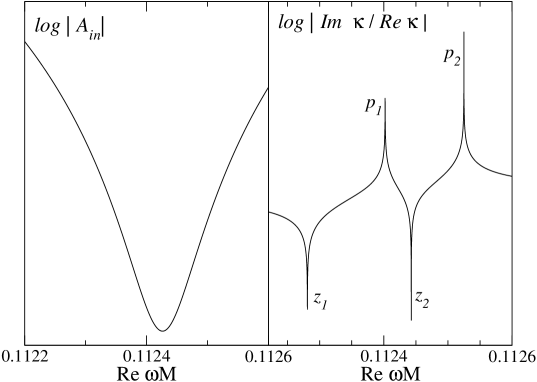
Figure 6: A graph of the incoming amplitude $A_{\rm in}$ vs the real part of the frequency. In the left panel we see a standard “Breit-Wigner resonance.” The right panel illustrates the properties of the phase of the ration of the asymptotic amplitudes. We use the location of the two poles and zeros to deduce the frequency and damping rate of a long-lived pulsation mode.

To devise a better scheme for determining the damping rate of a very long-lived QNM, we employ the two general properties we deduced earlier. From these it is clear that, if we have a zero of $A_{\rm in}$ close to the real frequency axis, there must also be a zero of $A_{\rm out}$ on the opposite side of the axis. How does that alter the above results? Close to a zero of $A_{\rm out}$ we will have

$$A_{\rm out}(\omega)\sim(\omega-\bar{\omega}_{n})\ .$$ (209)

Then we immediately see that the absolute value of the ratio between the asymptotic amplitudes, $\kappa$, is a smooth, slowly varying function of the frequency. But if we consider its phase, we find some interesting and useful features. We get (for real $\omega$)

$$\kappa\approx\gamma{\omega-\alpha_{n}+i\beta_{n}\over\omega-\alpha_{n}-i\beta_{n}}$$ (210)

where $\gamma=\gamma_{r}+i\gamma_{i}$ is a complex “constant,” and therefore

$${{\rm Im}\ \kappa\over{\rm Re}\ \kappa}\approx{\gamma_{i}[(\omega-\alpha_{n})^{2}-\beta_{n}^{2}]+2\gamma_{r}\beta_{n}(\omega-\alpha_{n})\over\gamma_{r}[(\omega-\alpha_{n})^{2}-\beta_{n}^{2}]-2\gamma_{i}\beta_{n}(\omega-\alpha_{n})}\ .$$ (211)

From this we see that, instead of having a singularity at $\omega=\alpha_{n}$ we now have a function with two zeros and two poles on the real frequency axis, cf. Fig. 6. Provided that the calculation of the asymptotic amplitudes can be done with sufficiently high precision, the location of these zeros ($z_{1,2}$) and poles ($p_{1,2}$) can readily be deduced. Given this information one can show that

$$\alpha_{n} \approx {p_{1}p_{2}-z_{1}z_{2}\over p_{1}+p_{2}-z_{1}-z_{2}}$$ (212)

$$\beta_{n} \approx [\alpha_{n}(z_{1}+z_{2})-\alpha_{n}^{2}-z_{1}z_{2}]^{1/2}$$ (213)

$${\gamma_{r}\over\gamma_{i}} \approx {2\beta_{n}\over p_{1}+p_{1}-2\alpha_{n}}={1\over 2\beta_{n}}[2\alpha_{n}-z_{1}-z_{2}]\ .$$ (214)

It should be pointed out that one gets four equations for the real and imaginary parts of the QNM frequency, as well as the ratio $\gamma_{r}/\gamma_{i}$. The last equality above can therefore be used as a “sanity check” on the calculation. In essence, it provides information about the accuracy of the obtained quantitites.

In practise, this method works very well even when the imaginary part of the frequency is more than eight orders of magnitude smaller than the real part, cf. the results in Table 3.

References

- (1) A.S. Eddington, MNRAS 79 2 (1918).
- (2) Proceedings of the SOHO 10/GONG 2000 Workshop: Helio- and asteroseismology at the dawn of the millennium, Ed: A. Wilson (ESA Publications Division, 2001).
- (3) A. Gautschy and H. Saio, Ann. Rev. Astron. Astrophys. 33 75 (1995).
- (4) N. Andersson and K. D. Kokkotas, Phys. Rev. Lett. 77 4134 (1996); MNRAS 299, 1059 (1998).
- (5) K. D. Kokkotas, T. Apostolatos and N. Andersson, MNRAS 302, 307 (2001).
- (6) S. Chandrasekhar, Phys. Rev. Lett. 24, 611 (1970).
- (7) J. L. Friedman, Commun. Math. Phys. 62, 247 (1978).
- (8) J. L. Friedman and B. F. Schutz, Astrophys. J. 222, 281 (1978).
- (9) N. Andersson, Ap. J. 502, 708 (1998).
- (10) J. L. Friedman and S. M. Morsink, Ap. J. 502, 714 (1998).
- (11) N. Andersson, K. D. Kokkotas, and N. Stergioulas, Ap. J. 516, 307 (1999).
- (12) G. Mendell, Ap. J. 380 530 (1991)
- (13) L. Bildsten and G. Ushomirsky Astrophys. J. Lett. 529 33 (2000).
- (14) L. Lindblom and G. Mendell, Phys. Rev. D 61, 104003 (2000).
- (15) P.B. Jones, Phys. Rev. Lett. 86 1384 (2001).
- (16) L. Lindblom and B.J. Owen, Effect of hyperon bulk viscosity on neutron-star r-modes preprint astro-ph/0110558
- (17) N. Andersson and G. L. Comer, Mon. Not. R. Astron. Soc. 328, 1129 (2001).
- (18) R. I. Epstein, Ap. J. 333, 880 (1988).
- (19) L. Lindblom and G. Mendell, Ap. J. 421, 689 (1994).
- (20) U. Lee, Astron. Astrophys. 303, 515 (1995).
- (21) R. Prix, in preparation (2002).
- (22) G. L. Comer, D. Langlois, and L. M. Lin, Phys. Rev. D 60, 104025 (1999).
- (23) N. Andersson and G. L. Comer, Phys. Rev. Lett. 24 241101 (2001).
- (24) V. V. Khodel, V. A. Khodel, and J. W. Clark, Nuc. Phys. A 679, 827 (2001).
- (25) C. W. Misner, K. S. Thorne, and J. A. Wheeler, Gravitation (Freeman Press, San Francisco, 1973).
- (26) B. Carter, “Relativistic fluid dynamics”, A. Anile and M. Choquet-Bruhat, Eds., Springer-Verlag (1989).
- (27) G. L. Comer and D. Langlois, Class. and Quant. Grav. 11, 709 (1994).
- (28) B. Carter and D. Langlois, Phys. Rev. D 51, 5855 (1995).
- (29) B. Carter and D. Langlois, Nucl. Phys. B 454, 402 (1998).
- (30) B. Carter and D. Langlois, Nucl. Phys. B 531, 478 (1998).
- (31) D. Langlois, A. Sedrakian, and B. Carter, Mon. Not. R. Astron. Soc. 297, 1189 (1998).
- (32) R. Prix, Phys. Rev. D 62, 103005 (2000)
- (33) N. Andersson and G. L. Comer, Class. and Quant. Grav. 18, 969 (2001).
- (34) T. Regge and J. A. Wheeler, Phys. Rev. 108, 1063 (1957).
- (35) L. Lindblom and S. L. Detweiler, Ap. J. Supplement Series 53, 73 (1983).
- (36) S. L. Detweiler and L. Lindblom, Ap. J. 292, 12 (1985).
- (37) A. F. Andreev and E. P. Bashkin, Sov. Phys. JETP 42 (1), 164 (1975).
- (38) R. Prix, G. L. Comer, and N. Andersson, Astron. Astrophys., 381 178 (2002).
- (39) O. Sjöberg, Nucl. Phys. A 265, 511 (1976).
- (40) A. Akmal, V.R. Panharipande and D.G. Ravenhall, Phys Rev C 58, 1804 (1998)
- (41) K. D. Kokkotas and B. F. Schutz, Mon. Not. R. Astron. Soc. 268, 1230 (1992).
- (42) A. Reisenegger and P. Goldreich, Ap. J. 395, 240 (1992).
- (43) A. Sedrakian and I. Wasserman, Phys. Rev. D 63, 024016 (2000).
- (44) W. Unno, Y. Osaki, H. Ando and H. Shibahashi Nonradial oscillations of stars (University of Tokyo Press, 1989)
- (45) L. M. Franco, B. Link and R. I. Epstein, Ap. J. 543 987 (2000).
- (46) D. Hartmann, K. Hurley and M. Niel Ap. J. 387, 622 (1992).
- (47) http://www.astro.cf.ac.uk/pub/B.Sathyaprakash/euro
- (48) F. J. Zerilli, Phys. Rev. D 2, 2141 (1970).
- (49) E. W. Leaver, Proc. Roy. Soc. London A 402, 285 (1985).
- (50) E. W. Leaver, J. Math. Phys. 27, 1238 (1986).
- (51) N. Andersson, K. D. Kokkotas, and B. F. Schutz, Mon. Not. R. Astron. Soc. 280, 1230 (1996).