Basic Principles of 4D Dilatonic Gravity and Some of Their Consequences for Cosmology, Astrophysics and Cosmological Constant Problem

Abstract

We present a class of simple scalar-tensor models of gravity with one scalar field (dilaton $\Phi$) and only one unknown function (cosmological potential $U(\Phi)$). These models might be considered as a stringy inspired ones with broken SUSY. They have the following basic properties: 1) Positive dilaton mass, $m_{{}_{\Phi}}$, and positive cosmological constant, $\Lambda$, define two extremely different scales. The models under consideration are consistent with the known experimental facts if $m_{{}_{\Phi}}>10^{-3}\,{\rm eV}$ and $\Lambda=\Lambda^{obs}\sim 10^{-56}\,{\rm cm}^{-2}$. 2) Einstein weak equivalence principle is strictly satisfied and extended to scalar-tensor theories of gravity by using a novel form of principle of “constancy of fundamental constants”. 3) The dilaton plays simultaneously roles of an inflation field and a quintessence field and yields a sequential hyper-inflation with a graceful exit to asymptotic de Sitter space-time, which is an attractor, and is approached as $\exp(-\sqrt{3\Lambda^{obs}}\,ct/2)$. The time duration of the inflation is $\Delta t_{infl}\sim m_{{}_{\Phi}}^{-1}$. 4) Ultra-high frequency ($\omega_{{}_{\Phi}}\sim m_{{}_{\Phi}}$) dilatonic oscillations take place in the asymptotic regime. 5) No fine tuning. (The Robertson-Walker solutions of general type have the above properties.) 6) A novel adjustment mechanism for the cosmological constant problem seems to be possible: the huge value of the cosmological constant in the stringy frame is rescaled to its observed value by dilaton after transition to the phenomenological frame.

PACS number(s): 04.50.+h, 04.40.Nr, 04.62.+v

I Introduction

The recent astrophysical observations of the type Ia supernovae Ia , CMB CMB , gravitational lensing and galaxies clusters’ dynamics (see the review articles CosmTri and the references therein) gave us strong and independent indications of existence of a new kind of dark energy in the Universe needed to explain the accelerated expansion and other observed phenomena. Although we are still not completely confident in these new observational results, it is worth trying to combine them with the old cosmological problems. Most likely, the conclusion one would reach is that a further generalization of the well established fundamental laws of physics and, in particular, of laws of gravity, is needed Snowmass .

At present, general relativity (GR) is the most successful theory of gravity at scales of laboratory, Earth-surface, Solar-System and star-systems. It gives quite good description of gravitational phenomena in the galaxies and at the scale of the whole Universe WW . Nevertheless, without some essential changes of its structure and basic notions, or without introducing some unusual matter and/or energy, GR seems to be unable to explain:

$\bullet$ the rotation of galaxies C ,

$\bullet$ the motion of galaxies in galactic clusters C ,

$\bullet$ physics of ultra-early Universe WW ; C ,

$\bullet$ the inflation Snowmass ; C ; inflation ,

$\bullet$ the initial singularity problem,

$\bullet$ the famous vacuum energy problem Weinberg , and

$\bullet$ the present-day accelerated expansion of the Universe Ia -Snowmass .

The most promising modern theories of gravity, like super gravity (SUGRA) and (super)string theories ((S)ST) Strings , having a deep theoretical basis, incorporate naturally GR. Unfortunately, they are not developed enough to allow a real experimental test, and introduce a large number of new fields without any direct experimental evidence and phenomenological support.

Therefore, it seems meaningful to look for some minimal extension of GR which is compatible with the known gravitational experiments, promises to overcome at least some of the above problems, and may be considered as a phenomenologically supported and necessary part of some more general modern theory.

In the present article we consider such a minimal model, which we call a four-dimensional-dilatonic-gravity (4D-DG). Up to now, this model has not attracted much attention. The investigation of 4D-DG was started by O’Hanlon as early as in 1974 OHanlon in connection with Fujii’s theory of the massive dilaton Fujii , but without any relation to the cosmological constant problem or other problems in cosmology and astrophysics. A similar model appears in the $D=5$ Kaluza-Klein theories Fujii97 . The relation of this model with cosmology and the cosmological constant problem was studied in F00 , where it was named a minimal dilatonic gravity (MDG). Possible consequences of 4D-DG for boson star structure were studied in PF2 . Some basic properties of 4D-DG were considered briefly in E-F_P in the context of general scalar tensor theories. There, the exceptional status of the 4D-DG among other scalar-tensor theories was stressed and a theory of cosmological perturbations for 4D-DG was sketched.

A wider understanding of dilatonic gravity as a metric theory of gravity in different dimensions with one non-matter scalar field can be found in the recent review article Odintsov . There, one can also find many examples of such models and a description of corresponding quantum effects. In contrast, we use the term 4D-DG only for our specific model.

In this article, we give a detailed consideration of the basic principles of the 4D-DG model, its experimental grounds, and some of its possible applications to astrophysics, cosmology and the cosmological constant problem. We believe that further developments of this model will yield a more profound understanding both of theory of gravity and of modern theories for unifying fundamental physical interactions. The 4D-DG model seems to give an interesting alternative for further development of these theories on real physical grounds.

In Section II, we consider briefly the modern foundations of scalar-tensor theories of gravity. In particular, we outline their connection with the universal sector of string theories and introduce our basic notations.

Section III is devoted to the role of Weyl’s conformal transformations outside the tree-level approximation of string theory. We discuss in detail the choice of frame and consider three distinguished frames: Einstein frame, cosmological constant frame and twiddle frame. Then, after a short review of basic properties of phenomenological frame, we discuss the problem of the choice of one of these distinguished frames as a phenomenological frame. Using some novel form of principle of “constancy of fundamental constants,” we choose the twiddle frame for phenomenological frame, thus arriving at our 4D-DG model in four-dimensional space-time.

In Section IV, we describe in detail our model.

There, we introduce a new system of cosmological units based on the observable value of cosmological constant $\Lambda^{obs}$ and dimensionless Planck number $P=\sqrt{\Lambda^{obs}}L_{{}_{Pl}}\approx 10^{-61}$, where $L_{{}_{Pl}}$ is Planck length.

Then we consider the basic properties of vacuum states in 4D-DG and the properties of admissible cosmological potentials. We show that the mass of dilaton in 4D-DG must have nonzero value.

In Section V, the weak field approximation for static system of point particles in 4D-DG is considered. We discuss the equilibrium between Newtonian gravity and weak anti-gravity, the constrains on the mass of dilaton from Cavendish-type experiments, the basic Solar System gravitational effects (Nordtvedt effect, time delay of electromagnetic pulses, perihelion shift) and possible consequences of big dilaton mass for star structure.

Section VI is devoted to some applications of 4D-DG in cosmology. We consider Robertson-Walker metric in 4D-DG, different forms of novel basic equations for evolution of Universe, energetic relations and some mathematical notions, needed for analysis of this evolution.

Then we derive the general properties of solutions in 4D-DG Robertson-Walker Universe and show the existence of asymptotic de Sitter regime with ultra-high frequency oscillations for all solutions, and the existence of initial inflation with dilaton field as inflation field. We obtain novel 4D-DG formulae for the number of e-folds and time duration of the inflation, the latter turns out to be related with the mass of dilaton via some new sort of quantum-like uncertainty relation.

In sharp contrast to standard inflation models and known quintessence models, the mass of the scalar field in 4D-DG (i.e., the mass of dilaton) is supposed to be very large, most probably in the TeV domain.

In addition, we give a solution of the inverse cosmological problem in 4D-DG. This solution differs significantly from the ones in other cosmological models.

The history of science teaches us that in the cases when a solution of some problem is not found for a long time, it is useful to reformulate the problem and look for some new approach to it. The essence of the cosmological constant problem is to find a physical explanation of the extremely small value of Planck number. This number connects the observed small value of the cosmological constant and the huge value of this quantity predicted by quantum field theory . On the other hand, it turns out that the same Planck number is related to the ratio of the classical action in the Universe and the Planck constant $\hbar$. In Section VII, we give very crude estimates for the amount of classical action accumulated during the evolution of the Universe after inflation in the matter sector and in 4D-DG gravi-dilaton sector. Then we describe qualitatively a novel idea for solution of the cosmological constant problem. It turns out that one can have a huge cosmological constant in basic stringy frame, due to the quantum vacuum fluctuation, but after transition to phenomenological frame this value is rescaled by the vacuum value of the dilaton field to the observed small positive cosmological constant through Weyl conformal transformation.

In the concluding Section VIII, we discuss some open problems of 4D-DG.

Mathematical proofs of some important statements are given in Appendices A and B.

II The Scalar-Tensor Theories of Gravity and Their Modern Foundations

Most likely, the minimal extension of GR must include at least one new scalar-field-degree of freedom. Indeed, such a scalar field is an unavoidable part of all promising attempts to generalize GR, starting with the first versions of Nordström and Kaluza-Klein-type theories, scalar-tensor theories of gravity, SUGRA, (S)ST (in all existing versions), M-theory, etc. In these modern theories, there is a universal sector, which we call in short a gravi-dilaton sector. Using the well known Landau-Lifschitz conventions, we write its action in some basic frame (BF) in the following most general form:

$${\cal A}_{g\phi}=\!-{c\over{2\kappa}}\!\int\!\!d^{D}x\sqrt{|{\bf g}|}\bigl{(}F(\phi)R\!-\!4Z(\phi)(\nabla\phi)^{2}\!+\!2\Lambda(\phi)\bigr{)}.$$ (1)

The contribution of the scalar field $\phi$ to the action of the theory can be described in different (sometimes physically equivalent) ways, by choosing different functions $F(\phi),Z(\phi)$ and $\Lambda(\phi)$ (which are not fixed a priory). If the basic frame is to be considered as a physical frame, the coefficients $F(\phi)$ and $Z(\phi)$ have to obey the general requirements $F(\phi)>0$ and $Z(\phi)\geq 0$. These conditions ensure non-negativity of the kinetic energy of graviton and dilaton. (The negative values of the function $F(\phi)$ correspond to anti-gravity, and a zero value yields infinite effective gravitational constant.)

In addition to the gravi-dilaton sector, we assume that there exists some matter sector with spinor fields $\psi$, gauge fields $A$, $\ldots$, relativistic fluids, etc., and action:

$${\cal A}_{matt}={1\over c}\!\int\!\!d^{D}x\sqrt{|{\bf g}|}\,{\cal L}(\psi,\nabla\psi;A,\nabla A;...;g_{\mu\nu},\phi).$$ (2)

Then the variation of the total action, ${\cal A}_{tot}={\cal A}_{g\phi}+{\cal A}_{matt}$, with respect to the metric $g_{\mu\nu}$ and the dilaton $\phi$ (after excluding the scalar curvature $R$ from the variational equation for scalar field in the case $F_{,_{\phi}}\neq 0$) yields the following field equations :

$$FG_{\mu\nu}={\kappa\over{c^{2}}}T_{\mu\nu}+\hskip 160.75789pt$$

$$4Z\!\left(\!\phi_{\!,_{\mu}}\phi_{,_{\nu}}\!-\!{1\over 2}\!\left(\nabla\phi\right)^{2}\!g_{\mu\nu}\!\right)\!\!+\!\left({\nabla_{\mu}\nabla_{\nu}\!-\!g_{\mu\nu}{\square}}\right)F\!+\!\Lambda(\phi)g_{\mu\nu},$$

$$J\,{\square}\phi+{1\over 2}J_{,_{\phi}}\left(\nabla\phi\right)^{2}+V_{\!,_{\phi}}={1\over{D\!-\!1}}\,{\kappa\over{c^{2}}}\,F_{\!,_{\phi}}\Theta.\hskip 55.48277pt$$ (3)

Hereafter, the comma denotes partial derivative with respect to the corresponding variable and

$$J(\phi)=F^{2}_{\!,_{\phi}}+4{{D\!-\!2}\over{D\!-\!1}}FZ,\hskip 113.81102pt$$

$$V(\phi)={{D\!-\!2}\over{D\!-\!1}}F(\phi)\Lambda(\phi)-2\int\Lambda(\phi)F_{\!,_{\phi}}(\phi)d\phi,\hskip 27.03003pt$$

$$\Theta=T+(D\!-\!2)\left(\ln{}_{{}_{S}\!}F\right){}_{\!\!,_{\phi}}{\cal L}_{\!,_{\phi}}.\hskip 105.2751pt$$ (4)

The tensor $T_{\nu\mu}={2\over{\sqrt{|{\bf g}|}}}{{\delta{\cal L}}\over{\delta{g^{\mu\nu}}}}$ is the standard energy-momentum tensor of matter, and $T$ is its trace.

In addition, we have two relations:

$${{D\!-\!2}\over 2}\!\left(4Z\left(\nabla\phi\right)^{2}\!-\!FR\right)\!+\!(D\!-\!1){\square}F\!-\!D\Lambda\!=\!{\kappa\over{c^{2}}}T,$$ (5)

$$F_{\!,_{\phi}}R+8Z{\square}\phi+4Z_{\!,_{\phi}}\left(\nabla\phi\right)^{2}+2\Lambda_{\!,_{\phi}}=2{\kappa\over{c^{2}}}{\cal L}_{\!,_{\phi}}.$$ (6)

The first one is obtained from the trace of the generalized Einstein equation in (3). One can derive the second one from the system (3), but actually it is a direct result of the variation of the total action with respect to the dilaton field $\phi$. Nevertheless, in the case $F_{,_{\phi}}\neq 0$, we consider the second of the relations in (3) as a field equation for the dilaton $\phi$, instead of the relation (6).

There have been many attempts to construct a realistic theory of gravity with action (1), starting with Jordan-Fierz-Brans-Dicke theory of variable gravitational constant and its further generalizations. The so called scalar tensor theories of gravity BD have been considered as a most natural extension of GR Damoor+ from phenomenological point of view. Different models of this type have been used in the inflationary scenario inflation and in the more recent quintessence models Q . For the latest developments of the scalar-tensor theories in connection with the accelerated expansion of the Universe, one can consult the recent article E-F_P .

It is natural to look for a more fundamental theoretical evidence in favor of the action (1).

For example, a universal gravi-dilaton sector described by action of type (1) appears in minimal $D=4$, $N=1$ SUGRA. (See the recent article Townsend and the references therein.) In this model, the scalar field $\phi$ belongs to chiral supermultiplet, $F(\phi)=1$, $Z(\phi)=2$ and, to obtain a general potential in a form $\Lambda(\phi)=(w^{\prime})^{2}-\beta^{2}w^{2}+\xi^{2}h$, one needs to include one vector multiplet, which is coupled to the scalar field through the real function $h(\phi)$. The function $w(\phi)$ describes the corresponding real superpotential, $\beta$ is a phenomenological constant related to the matter equation of state, and $\xi$ is Fayet-Illiopoulos constant. Similar potentials $\Lambda(\phi)$ appear in $N=8$ SUGRA, as well as in the brane world picture Townsend .

The action of type (1) is common for all modern attempts to create a unified theory of all fundamental interactions based on stringy idea.

Indeed, consider the universal sector of the low energy limit (LEL) of (S)ST in stringy frame (SF), which is the basic frame in this case. The gravi-dilaton Lagrangian is:

$${}_{{}_{S}\!}L_{{}_{LEL}}^{(0)}\sim\sqrt{|{}_{{}_{S}\!}{\bf g}|}e^{-2\phi}\left({}_{{}_{S}\!}R+4\,{}_{{}_{S}\!}(\nabla\phi)^{2}+2{}_{{}_{S}\!}C_{\Lambda}^{(0)}\right).$$

We use the upper index ${(0)}$ to label the tree-level-approximation quantities,

$${}_{{}_{S}\!}F^{(0)}(\phi)=-{}_{{}_{S}\!}Z^{(0)}(\phi)=e^{-2\phi},\,\,\Lambda^{(0)}(\phi)={}_{{}_{S}\!}C_{\Lambda}^{(0)}e^{-2\phi},$$ (7)

and the “cosmological constant” is ${}_{{}_{S}\!}C_{\Lambda}^{(0)}={\frac{D-26}{3\alpha^{\prime}}}$ for bosonic strings, and ${}_{{}_{S}\!}C_{\Lambda}^{(0)}\sim(D-10)$ for superstrings, and $\alpha^{\prime}$ is Regge slope parameter. Including the contribution of all loops, one arrives at the following general form of LEL stringy gravi-dilaton Lagrangian:

$${}_{{}_{S}\!}L_{{}_{LEL}}\sim\hskip 85.35826pt$$

$$\sqrt{|{}_{{}_{S}\!}{\bf g}|}e^{-2\phi}\left({}_{{}_{S}\!}C_{g}(\phi){}_{{}_{S}\!}R+4\,{}_{{}_{S}\!}C_{\phi}(\phi)(\nabla\phi)^{2}+2\,{}_{{}_{S}\!}C_{\Lambda}(\phi)\right),$$ (8)

where

$${}_{{}_{S}\!}C_{...}(\phi)\!=\!\sum_{n=0}^{\infty}{}_{{}_{S}\!}C_{...}^{(n)}\!\exp(2n\phi)$$ (9)

are unknown functions with ${}_{{}_{S}\!}C_{g}^{(0)}=1$, ${}_{{}_{S}\!}C_{\phi}^{(0)}=1$. (See the references Pol_Dam where functions $B_{...}(\phi)=e^{-2\phi}C_{...}(\phi)$ were introduced. Here dots … stand for $g$, or $\phi$.)

The SF cosmological potential ${}_{{}_{S}\!}\Lambda(\phi)$ must be zero in the case of exact supersymmetry, but in the real world such nonzero term may originate from SUSY breaking due to super-Higgs effect, gaugino condensation, or may appear in some more complicated, still unknown, way. Its form is not known exactly, too. At present, the only clear thing is that we are not living in the exactly supersymmetric world and one must somehow break down the SUSY. We consider this phenomenological fact as a sufficient evidence in favor of the assumption that in a physical theory which describes the real world, ${}_{{}_{S}\!}\Lambda(\phi)\neq 0$ both for critical and for non-critical fundamental strings. Thus, we use the nonzero cosmological potential $\Lambda(\phi)$ to describe pnenomenologically the SUSY breaking.

Hence, to fix the LEL gravi-dilaton Lagrangian in SF, we have to know the three dressing functions of the dilaton: ${}_{{}_{S}\!}C_{g}(\phi)$, ${}_{{}_{S}\!}C_{\phi}(\phi)$, and ${}_{{}_{S}\!}C_{\Lambda}(\phi)$.

This way, we arrive at a scalar-tensor theory of gravity of most general type (1) with some specific stringy-determined functions:

$${}_{{}_{S}\!}F(\phi)={}_{{}_{S}\!}C_{g}(\phi)e^{-2\phi},\,\,\,{}_{{}_{S}\!}Z(\phi)=-{}_{{}_{S}\!}C_{\phi}(\phi)e^{-2\phi},$$

$${}_{{}_{S}\!}\Lambda(\phi)={}_{{}_{S}\!}C_{\Lambda}(\phi)e^{-2\phi}.\hskip 42.67912pt$$ (10)

In this paper, we consider general scalar theories of gravity in this stringy context. Although we use stringy terminology, our considerations are valid for all scalar-tensor theories. We choose this language for describing our model simply because the (S)ST, their brane extensions, and M-theory at present are the most popular candidates for “theory of everything”.

In addition to the gravi-dilaton sector, in these modern theories, there are many other fields: axion field, gauge fields, different spinor fields, etc., which we do not consider here in detail. For spinor fields $\psi$ and for gauge fields $A_{\mu}$, one has to add to the total Lagrangian of the theory terms that in flat space-time ${\cal M}^{D}$ have the form

$${}_{{}_{S}\!}C_{\psi}(\phi)e^{-2\phi}\,\,\bar{\psi}\gamma^{\mu}\partial_{\mu}\psi={}_{{}_{S}\!}B_{\psi}(\phi)\,\,\bar{\psi}\gamma^{\mu}\partial_{\mu}\psi,$$

$${}_{{}_{S}\!}C_{m}(\phi)e^{-2\phi}\,\,m\bar{\psi}\psi={}_{{}_{S}\!}B_{m}(\phi)\,\,m\bar{\psi}\psi,$$

$${}_{{}_{S}\!}C_{e}(\phi)e^{-2\phi}\,\,e\,A_{\mu}\bar{\psi}\gamma^{\mu}\psi={}_{{}_{S}\!}B_{e}(\phi)\,\,e\,A_{\mu}\bar{\psi}\gamma^{\mu}\psi,$$

$${}_{{}_{S}\!}C_{{}_{F}}(\phi)e^{-2\phi}\,\,F_{\mu\nu}F^{\mu\nu}={}_{{}_{S}\!}B_{{}_{F}}(\phi)\,\,F_{\mu\nu}F^{\mu\nu}$$ (11)

with unknown coefficients ${}_{{}_{S}\!}C_{...}(\phi)$ of type (9). The connection of these terms with the real matter is not clear at present. Therefore, we describe the real matter phenomenologically, i.e., at the same standard manner as in GR, using the available experimental information.

III The Transition to New Frames Using Weyl Conformal Transformations

After Weyl conformal transformation:

$$g_{\mu\nu}\rightarrow e^{-2\sigma(\phi)}g_{\mu\nu}$$ (12)

to some new conformal frame, ignoring a surface term which is proportional to $2(D-1)\sqrt{|{\bf g}|}\,{}_{{}_{S}\!}Fe^{(D\!-\!2)\sigma}g^{\mu\nu}\sigma_{,_{\nu}}$, we obtain the stringy LEL Lagrangian (in $D$ dimensions) in the form

$$L_{{}_{LEL}}\sim\sqrt{|{\bf g}|}\left(F(\phi)R-4Z(\phi)(\nabla\phi)^{2}+2\Lambda(\phi)\right)$$ (13)

where

$$F(\phi)={}_{{}_{S}\!}F(\phi)e^{(D-2)\sigma(\phi)},\,Z(\phi)={}_{{}_{S}\!}\tilde{Z}(\phi)e^{(D-2)\sigma(\phi)},$$

$$\Lambda(\phi)={}_{{}_{S}\!}\Lambda(\phi)e^{D\sigma(\phi)},\hskip 130.88284pt$$ (14)

$${}_{{}_{S}\!}\tilde{Z}(\phi)={}_{{}_{S}\!}Z(\phi)+\Delta{}_{{}_{S}\!}Z(\phi),\hskip 96.73918pt$$

$$\Delta\!{}_{{}_{S}\!}Z(\phi)\!=-{{D\!-\!1}\over 2}\,{}_{{}_{S}\!}F\!\left(\left(\ln\!{}_{{}_{S}\!}F\right){}_{\!\!,_{\phi}}\,\sigma_{\!,_{\phi}}\!+\!{{(D\!-\!2)}\over 2}\,\sigma_{\!,_{\phi}}^{2}\!\right).$$ (15)

Combining relations (14) and (15), we obtain the transformation law

$${Z\over F}\!=\!{{{}_{{}_{S}\!}Z}\over{{}_{{}_{S}\!}F}}\!-\!{{D\!-\!1}\over 2}\left(\ln\!{}_{{}_{S}\!}F\right){}_{\!\!,_{\phi}}\sigma_{\!,_{\phi}}\!-\!{{(D\!-\!1)(D\!-\!2)}\over 4}\left(\sigma_{\!,_{\phi}}\right)^{2}.$$ (16)

The transition functions $\sigma$ have the following pseudo-group property:

If ${}_{{}_{1}\!}\sigma_{\!{}_{0}}$ and ${}_{{}_{2}\!}\sigma_{\!{}_{0}}$ describe transitions from some initial frame 0F to some new frames 1F and 2F according Eq. (12), (i.e., ${}_{{}_{I}}g_{\mu\nu}=e^{-2{}_{{}_{I}}\!\sigma\!{}_{{}_{J}}(\phi)}{}_{{}_{J}}g_{\mu\nu}$ for $I,J=0,1,2;$) then the transition from 1F to 2F is given by

$${}_{{}_{2}\!}\sigma_{\!{}_{1}}={}_{{}_{2}\!}\sigma_{\!{}_{0}}-{}_{{}_{1}\!}\sigma_{\!{}_{0}}\,.$$ (17)

The relations (14)–(16) give a specific induced representation of Weyl transformations (12) which acts on coefficients $F$, $Z$, and $\Lambda$ in the Lagrangian (13) and has the corresponding pseudo-group property.

As seen from the above relations, for known stringy-dressed coefficients ${}_{{}_{S}\!}F(\phi)$, ${}_{{}_{S}\!}Z(\phi)$ and given ${}_{{}_{S}\!}\tilde{Z}(\phi)$, one obtains in general (i.e., for $D>2$) two transition functions:

$$\sigma^{\pm}(\phi)={{1}\over{D\!-\!2}}\left(-\ln{}_{{}_{S}\!}F(\phi)\pm{2\over{\sqrt{D\!-\!1}}}\tilde{S}(\phi)\right)\,,$$ (18)

where $\tilde{S}(\phi)=\int d\phi\sqrt{\Delta({}_{{}_{S}\!}F(\phi),{}_{{}_{S}\!}Z(\phi)-{}_{{}_{S}\!}\tilde{Z}(\phi))}$, and the following important combination of functions have been introduced:

$$\Delta(F,Z)={{D\!-\!1}\over{4F^{2}}}J={{D\!-\!1}\over{4}}\left(\ln F\right)_{\!,_{\phi}}^{2}+(D\!-\!2){Z\over F}$$ (19)

with normalization

$$\Delta\left({}_{{}_{S}\!}F^{(0)}(\phi),{}_{{}_{S}\!}Z^{(0)}(\phi)\right)\equiv 1$$ (20)

and basic property

$$\Delta(F,Z)\geq 0\,,$$ (21)

when $4(D\!-\!2){Z\over F}\geq-(D\!-\!1)\left(\ln F\right)_{\!,_{\phi}}^{2}$.

III.1 The Choice of Frame

Now the following question arises: what frame to choose – stringy, Einstein, or some other frame ?

This is still an open problem and in the literature one can find basically different statements (see the first article in Faraoni for a large amount of references and their detailed analysis). In the present article, we try to answer this question by analyzing the situation from different points of view and making a series of simple steps in the direction which seems to us to be the right one from phenomenological point of view.

III.1.1 Are All Frames Equivalent ?

Some authors consider the change of frame as a formal mathematical procedure which is physically irrelevant. According to this point of view, all frames are physically equivalent, at least up to possible singularities in the corresponding transition functions.

The whole wisdom in this statement is related to the rather trivial observation, that if we are given some physical theory, we have the freedom to change locally variables in any convenient way. Then we can transform to the new frame any physical law, sometimes ignoring the fact that in the new frame this law may have a strange and unusual form from physical point of view. This means that one may consider every given physical theory in different local coordinates in the corresponding (field) phase space.

This physically trivial statement neglects one of the most important features of the physical problems, even when they are well formulated. Namely, for each problem there exists, as a rule, a unique “coordinate system” which is proper for the solution of the problem. It is well known that the most important technical issue for solving any physical problem is to find this “proper coordinate system”.

In the language of mathematics, this means that we have to find the “unique” global uniformization variables for the problem under consideration. For real problems, this might be a nontrivial and very complicated mathematical issue.

The naive change of frame may alter the global properties of the physical system because of the following reasons:

1) Weyl transformations (12) do not form a group, but a pseudo-group and, in general, they do change the global structure of space-time and of the physical theory. Typically, only a part of the space-time manifold ${}_{{}_{1}}{\cal M}^{(D)}$ of the initial frame 1F is smoothly mapped onto some part of the space-time manifold ${}_{{}_{2}}{\cal M}^{(D)}$ of the frame 2F. In addition, (as seen, e.g., from formula (18)), the mapping may be not one-to-one.

2) Under Weyl transformation (12), the Lagrangian acquires a surface term proportional to

$$2(D-1)\oint d\Sigma^{\mu}\sigma_{,_{\mu}}\sqrt{|{\bf g}|}\,{}_{{}_{S}\!}F\,e^{(D\!-\!2)\sigma}$$

that we ignore. In space-times with boundary, this may lead to a physically non-equivalent theory.

There exists one more argument for using different frames. In the case of the theories we consider in the present article, the very physical problem is still not completely fixed. It seems quite possible that, looking at it in different frames, one can find some new physical grounds which can help to restrict in a proper way the a priory existing possibilities and to justify the unknown theoretical ingredients.

III.1.2 Is the Basic Frame Enough for Doing Physics ?

If one firmly believes in beautiful theoretical constructions like (super)strings, branes, or in some other physical theory, one may intend to prescribe a direct physical meaning to the variables in which these theories look beautiful and simple. Therefore, one may consider the basic frame (SF – for string theories) as a physical one, i.e., as a frame in which we see directly the properties of the real world. It seems obvious that one need not accept such additional hypotheses, i.e., the basic variables of the fundamental theory may have only indirect relation with the real world. Then defining the basic principles for choosing physical variables becomes an important theoretical issue. These principles must be based on some phenomenological facts.

In the case of string theory, the wrong sign of the kinetic term in the SF-LEL-Lagrangian is enough to consider the basic stringy frame as a non-physical one. Otherwise, the theory would not have a stable ground state.

III.2 Three Distinguished Frames for Scalar-Tensor Theories

Looking at the basic formulae (14) and (15), it is not hard to understand that three simple choices of frame are possible: since under Weyl conformal transformation the functions ${}_{{}_{S}\!}F(\phi)$ and ${}_{{}_{S}\!}\Lambda(\phi)$ have a linear and homogeneous transformation law, one can choose the function $\sigma(\phi)$ in such a way that:

i) $F(\phi)={\rm const}>0$; or

ii) $\Lambda(\phi)={\rm const}$ ($>0$ when ${}_{{}_{S}\!}\Lambda(\phi)>0$).

The third possibility for a simple choice of conformal gauge is to use the non-homogeneous linear transformation law (15) for the function ${}_{{}_{S}\!}Z(\phi)$ and to impose the conformal gauge fixing condition:

iii) $Z(\phi)={\rm const}=0$.

It is remarkable that in each of these three cases one can reduce the number of the unknown functions in the gravi-dilaton sector to one (by using a proper re-definition of the dilaton field). That is why, before discussing the choice of some frame as the physical one, we describe briefly their properties.

III.2.1 Einstein Frame

The most popular and well known frame is Einstein frame (EF), defined according to the first choice (i) when $D\!>\!2$. (If $D=2$ and ${}_{{}_{S}\!}F(\phi)\neq{\rm const}$, EF does not exist.) The transition from SF to EF is described by transition function ${}_{{}_{E}\!}\sigma{}_{\!{}_{S}}=-{{1}\over{D\!-\!2}}\ln{}_{{}_{S}\!}F$ and coefficients

$${}_{{}_{E}\!}F(\phi)\equiv 1,\,\,{}_{{}_{E}\!}Z(\phi)={1\over{D\!-\!2}}\Delta\left({}_{{}_{S}\!}F(\phi),{}_{{}_{S}\!}Z(\phi)\right),\,\,$$

$${}_{{}_{E}\!}\Lambda(\phi)={}_{{}_{S}\!}F(\phi)^{-{{D}\over{D-2}}}{}_{{}_{S}\!}\Lambda(\phi).\hskip 36.98866pt$$ (22)

For tree-level string approximation, one easily obtains the familiar LEL coefficients

$${}_{{}_{E}\!}Z^{(0)}(\phi)={{1}\over{D-2}}={\rm const}>0,\,{}_{{}_{E}\!}\Lambda^{(0)}(\phi)={}_{{}_{S}\!}C^{(0)}e^{{4\phi}\over{D-2}}.$$

For the general case of a dressed LEL Lagrangian, one has to re-define the dilaton field, introducing dimensionless EF-dilaton $\varphi$ according to the formula :

$$\varphi(\phi)=\varphi^{\pm}(\phi)=\pm\sqrt{{4\over{D\!-\!2}}}S(\phi)\ ,$$ (23)

where

$$S(\phi)=\int d\phi\sqrt{\Delta\left({}_{{}_{S}\!}F(\phi),{}_{{}_{S}\!}Z(\phi)\right)}$$ (24)

is real if the condition (21) is fulfilled for the dressed coefficients ${}_{{}_{S}\!}F(\phi)$ and ${}_{{}_{S}\!}Z(\phi)$.

The existence of two solutions $\varphi^{+}(\phi)=-\varphi^{-}(\phi)$ reflects the well known S-duality of string theory. In EF this duality corresponds to the invariance of the metric ${}_{{}_{E}\!}g_{\mu\nu}$ under a simple change of the sign of the dilaton field $\varphi$.

This way, we reach the final form (1) of the EF-LEL stringy Lagrangian with coefficients

$${}_{{}_{E}\!}F(\varphi)=1,\,\,{}_{{}_{E}\!}Z(\varphi)={1\over 4},\,\,{}_{{}_{E}\!}\Lambda(\varphi)=\Lambda^{obs}{}_{{}_{E}\!}U(\varphi)\ ,$$ (25)

where $\Lambda^{obs}$ is a constant which we choose to equals the positive observed cosmological constant, and the dimensionless EF cosmological potential is

$${}_{{}_{E}\!}U(\varphi)={{{}_{{}_{S}\!}\Lambda(\phi(\varphi))}\over{\Lambda^{obs}}}\bigl{(}{}_{{}_{S}\!}F(\phi(\varphi))\bigr{)}^{-{D\over{D\!-\!2}}},$$ (26)

$\phi(\varphi)$ being the inverse function to the function (23).

Now we have a standard EF-representation not only for the tree-level LEL, but for the entire dressed LEL stringy Lagrangian (8). Its EF representation reads

$${}_{{}_{E}\!}L_{{}_{LEL}}\sim\sqrt{|{}_{{}_{E}\!}{\bf g}|}\left({}_{{}_{E}\!}R-{}_{{}_{E}\!}(\nabla\varphi)^{2}+2\Lambda^{obs}{}_{{}_{E}\!}U(\varphi)\right).$$ (27)

In this frame

i) Dilaton degree of freedom is separated from Hilbert-Einstein term ($\sim R$) in the Lagrangian, and, to some extend, but not exactly, EF-fields’ coordinates play the role of normal coordinates for the gravi-dilaton sector.

ii) The EF-dilaton $\varphi$ looks like a normal matter scalar field with the right sign of its kinetic energy in the action (1) if the inequality (21) is fulfilled.

In the case of a negative function $\Delta({}_{{}_{S}\!}F(\phi),{}_{{}_{S}\!}Z(\phi))<0$, one is not able to introduce positive kinetic energy for a real EF-dilaton and the string theory in EF will not have a consistent physical interpretation.

This observation raises the question, is really EF the proper physical frame for (S)ST outside the tree-level approximation. To answer this question, one needs to know the total stringy dressed coefficients ${}_{{}_{S}\!}F(\phi)$ and ${}_{{}_{S}\!}Z(\phi)$, or at least one needs to have an independent proof of validity of condition (21). This is still an open problem, and further on we accept the hypothesis that the condition (21) is valid in the scalar-tensor theories under consideration.

iii) As a normal matter field, the EF-dilaton $\varphi$ is minimally coupled to gravity (i.e., to EF-metric tensor ${}_{{}_{E}\!}g_{\mu\nu}$), and respects Einstein WEP.

Hence, the EF-dilaton $\varphi$ may enter the matter Lagrangian of other matter fields in a rather arbitrary way without violation of WEP. The only consequence one can derive from WEP in this case is the metric character of gravity, described only by the EF metric ${}_{{}_{E}\!}g_{\mu\nu}$. One can consider a priory arbitrary interactions of the EF-dilaton $\varphi$ with other matter. For example, the theory does not exclude a priory interactions, described in EF by formulae analogous to Eq. (11) with proper coefficients ${}_{{}_{E}\!}C_{...}(\varphi)$. Because of the interpretation of the EF-dilaton $\varphi$ as an ordinary matter field, in this case one would be forced to explain the deviations of particle motion from geodesic lines (with respect to the metric ${}_{{}_{E}\!}g_{\mu\nu}$) by introducing some specific “dilatonic charge” (often called ”an interaction parameter”) which determines the interaction of dilaton with other matter fields.

iv) The cosmological potential ${}_{{}_{E}\!}U(\varphi)$ remains the only unknown function in the EF-gravi-dilaton sector, but the dependence of the matter Lagrangian ${}_{{}_{E}\!}{\cal L}_{...}(...,\varphi)$ on the EF-dilaton $\varphi$ is a new physical problem which one must solve to fix the theory. Here dots stay for other matter fields.

v) In the presence of additional matter of any other (i.e., different from dilaton $\varphi$) kind with action

$${}_{{}_{E}\!}{\cal A}{...}={1\over c}\!\int\!\!d^{D}x\sqrt{|{}_{{}_{E}\!}{\bf g}|}{}_{{}_{E}\!}{\cal L}_{...}(...,\varphi)\ ,$$

the usual GR field equations,

$$G_{\alpha\beta}={\kappa\over{c^{2}}}{}_{{}_{E}\!}T_{\alpha\beta},$$

$${}_{{}_{E}\!}{{\square}}\,\varphi+\Lambda^{obs}\!{}_{{}_{E}\!}U_{\!,_{\varphi}}={\frac{\kappa}{c^{2}}}({}_{{}_{E}\!}{\cal L}_{...})_{,_{\varphi}}\hskip 0.0pt$$ (28)

yield the usual energy-momentum conservation law, $\nabla_{\alpha}\,{}_{{}_{E}}\!T^{\alpha}_{\beta}=0$, for the total energy-momentum of the matter

$${}_{{}_{E}\!}T_{\alpha\beta}={2\over{\sqrt{|{}_{{}_{E}\!}{\bf g}|}}}{{\delta{}_{{}_{E}\!}{\cal L}_{...}}\over{\delta{}_{{}_{E}\!}{g^{\alpha\beta}}}}+\hskip 116.65646pt$$

$${{c^{2}}\over\kappa}\left(\varphi_{\!,_{\alpha}}\varphi_{\!,_{\beta}}\!-\!{1\over 2}\left(\nabla\varphi\right)^{2}\!{}_{{}_{E}\!}g_{\alpha\beta}\!+\!\Lambda^{obs}\!{}_{{}_{E}\!}U(\varphi){}_{{}_{E}\!}g_{\alpha\beta}\right)$$ (29)

and an additional relation – the EF version of Eq. (5):

$$R-\left(\nabla\varphi\right)^{2}+{{2D}\over{D\!-\!2}}\Lambda^{obs}\!{}_{{}_{E}\!}U(\varphi)+{\kappa\over{c^{2}}}{2\over{D\!-\!2}}{}_{{}_{E}\!}T_{...}=0,$$ (30)

where ${}_{{}_{E}\!}T_{...}$ is the trace of energy-momentum tensor of the additional matter in EF.

vi) As seen from Eq. (28), as a matter field in a fixed metric ${}_{{}_{E}\!}g^{\mu\nu}$, the EF-dilaton $\varphi$ has its own nontrivial dynamics determined by corresponding Klein-Gordon equation with cosmological potential ${}_{{}_{E}\!}U(\varphi)$ in a (curved) space-time ${\cal M}^{(1,3)}\{{}_{{}_{E}\!}g^{\mu\nu}\}$. Therefore, the EF-dilaton may be a variable field in homogeneous space-times with constant curvature (in particular, in a flat space-time).

vii) Because of the conservation of the total energy-momentum, without taking into account the EF-dilaton $\varphi$, we have to expect a violation of the conservation of energy-momentum of other matter if $({}_{{}_{E}\!}{\cal L}_{...})_{,_{\varphi}}\neq 0$, i.e., when the matter is a source for EF-dilaton $\varphi$ according to Eq. (28). Hence, the dilaton $\varphi$ is a source of other matter:

$$\nabla_{\mu}\,{}_{{}_{E}}\!T_{...}{}^{\mu}_{\nu}=-({}_{{}_{E}\!}{\cal L}_{...})_{,_{\varphi}}\varphi_{\nu}\,.$$ (31)

III.2.2 Brans-Dicke-Cosmological-Constant Frame

We call this new frame a $\Lambda$-frame ($\Lambda$F) and define it by using the second distinguished possibility for choice of frame (see subsection B). Now we impose the conformal gauge condition, ${}_{{}_{\Lambda}\!}\Lambda(\phi)={\rm const}$, and by choosing this constant equal to the observable value $\Lambda^{obs}$, we obtain ${}_{{}_{\Lambda}\!}\sigma=-{1\over D}\ln\left({{{}_{{}_{S}\!}\Lambda(\phi)}\over{\Lambda^{obs}}}\right)$ and

$${}_{{}_{\Lambda}\!}F(\phi)={}_{{}_{S}\!}F(\phi)\left({{{}_{{}_{S}\!}\Lambda(\phi)}/{\Lambda^{obs}}}\right)^{-{{D\!-\!2}\over D}},\,\,{}_{{}_{\Lambda}\!}\Lambda(\phi)=\Lambda^{obs},$$

$${{{}_{{}_{\Lambda}\!}Z}\over{{}_{{}_{\Lambda}\!}F}}={{{}_{{}_{S}\!}Z}\over{{}_{{}_{S}\!}F}}+{{D\!-\!1}\over{2D}}{{{}_{{}_{S}\!}\Lambda_{,_{\phi}}}\over{{}_{{}_{S}\!}\Lambda}}\left({{{}_{{}_{S}\!}F_{,_{\phi}}}\over{{}_{{}_{S}\!}F}}-{{D\!-\!2}\over{2D}}{{{}_{{}_{S}\!}\Lambda_{,_{\phi}}}\over{{}_{{}_{S}\!}\Lambda}}\right)\,.$$ (32)

After a re-definition of the $\Lambda$F-dilaton according to the formula

$$\chi={}_{{}_{\Lambda}\!}F(\phi)\,,$$ (33)

we obtain the final form of the $\Lambda$F-LEL stringy Lagrangian coefficients:

$${}_{{}_{\Lambda}\!}F(\chi)=\chi,\,\,\,{}_{{}_{\Lambda}\!}Z(\chi)=\omega(\chi)/\chi,\,\,\,{}_{{}_{\Lambda}\!}\Lambda(\chi)=\Lambda^{obs}\,,$$ (34)

where the Brans-Dicke coefficient is

$$\omega(\chi)=4\left(\phi^{\prime}\right)^{2}{{{}_{{}_{S}\!}Z}\over{{}_{{}_{S}\!}F}}+\hskip 128.0374pt$$

$$2{{D\!-\!1}\over{D}}\left(\ln{}_{{}_{S}\!}\Lambda\right)^{\prime}\left(\ln{}_{{}_{S}\!}F\right)^{\prime}-{(D\!-\!1)(D\!-\!2)\over{D^{2}}}\left(\left(\ln{}_{{}_{S}\!}\Lambda\right)^{\prime}\right)^{2},$$ (35)

$\phi(\chi)$ is the inverse to the function (33), and prime denotes differentiation with respect to $\ln\chi$.

For the tree-level LEL approximation, one obtains

$$\phi\!=\!-{D\over 4}\ln\chi\!+\!{\rm const},\,{}_{{}_{S}\!}F^{(0)}\!=\!-{}_{{}_{S}\!}Z^{(0)}\!\sim\!\chi^{D\over 2},\,{}_{{}_{S}\!}\Lambda^{(0)}\!\sim\!\chi^{D\over 2},$$

$$\omega^{(0)}={{D\!-\!2}\over 4}.\hskip 85.35826pt$$ (36)

Now we see that in $\Lambda$F the gravi-dilaton sector looks precisely like Brans-Dicke theory with nonzero cosmological constant, i.e., we have

$${}_{{}_{\Lambda}\!}L_{{}_{LEL}}\sim\sqrt{|{}_{{}_{\Lambda}\!}{\bf g}|}\left(\chi\,{}_{{}_{\Lambda}\!}R-\chi^{-1}\omega(\chi){}_{{}_{\Lambda}\!}(\nabla\chi)^{2}+2\Lambda^{obs}\right).$$ (37)

Hence, we can apply all well-studied properties of Brans-Dicke theory WW ; BD . to the part of (S)ST under consideration. We shall stress some well known properties of this theory which we need later:

i) In contrast to the EF-dilaton $\varphi$, the interactions of the $\Lambda$F-dilaton $\chi$ with the matter are completely fixed by $\Lambda$F Einstein WEP in the simplest possible way: to satisfy WEP in $\Lambda$F, the dilaton $\chi$ must not enter the $\Lambda$F-matter Lagrangian. Its influence on the matter is only indirect – it is due to the interaction (37) with the metric ${}_{{}_{\Lambda}\!}g_{\mu\nu}$ (which, in turn, must enter $\Lambda$F-matter Lagrangian minimally, i.e., as in GR).

Hence, in the entire $\Lambda$F-theory we have only one unknown function related to dilaton, namely the Brans-Dicke function $\omega(\chi)$.

ii) One obtains the field equations for $\Lambda$F theory by replacing in Eq. (3) the variable $\phi$ with $\chi$ and using (34) and the relations ${}_{{}_{\Lambda}\!}V_{,_{\chi}}\equiv 0$, ${}_{{}_{\Lambda}\!}J=1+4{{D\!-\!2}\over{D\!-\!1}}\omega(\chi)$, and ${}_{{}_{\Lambda}\!}\Theta={}_{{}_{\Lambda}\!}T$.

The additional relation (6) now reads

$$R+8\,\chi^{-1}\omega\,{\square}\chi+4\left(\chi^{-1}\omega\right)_{\!,_{\chi}}(\nabla\chi)^{2}=0\,.$$ (38)

iii) The $\Lambda$F-dilaton $\chi$ is not a matter field, but rather a part of the description of gravity. We have arrived at a purely dynamical metric theory of gravity with one scalar gravitational field Will . It plays the role of a variable effective gravitational constant: $G_{eff}=G_{N}/\chi$.

This seems to be much more in the spirit of string theory where graviton and dilaton appear in the same physical sector.

iv) If considered as a specific scalar field in a fixed metric ${}_{{}_{\Lambda}\!}g_{\mu\nu}$ (according to standard Brans-Dicke dynamics), $\Lambda$F-dilaton $\chi$ may still have space-time variations. For example, in homogeneous space-times and even in flat space-time ${\cal M}^{D}\{{}_{{}_{\Lambda}\!}g_{\mu\nu}\}$, one can have a variable field $\chi$.

In addition, in our stringy-inspired approach to Brans-Dicke theory with a cosmological constant, we obtain one more novel general property:

v) As seen from formula (35), the observable cosmological constant $\Lambda^{obs}$ does not enter explicitly Brans-Dicke function $\omega(\chi)$. The same holds for any common constant scale factor in the SF cosmological potential ${}_{{}_{S}\!}\Lambda(\phi)$. This is due to the dependence of $\omega(\chi)$ on the derivatives of $\ln{}_{{}_{S}\!}\Lambda$ and other functions with respect to $\ln\chi$. The two factors are absorbed in the $\Lambda$F metric ${}_{{}_{\Lambda}\!}g_{\mu\nu}$ and in the dilaton $\chi$ as described by formulae (12), (32), and (33). As a result, in the $\Lambda$F-LEL Lagrangian (37), the only remaining “free” parameter is $\Lambda^{obs}$.

As a consequence, when $D=4$, we discover a new symmetry: the Lagrangian (37) is form-invariant under rescaling of the SF cosmological potential ${}_{{}_{S}\!}\Lambda$ if $\omega(\chi)$ does not depend on the $\Lambda$F-dilaton $\chi$.

Indeed, let us consider a rescaling of the cosmological potential ${}_{{}_{S}\!}\Lambda$ with a constant factor $\lambda$:

$${}_{{}_{S}\!}\Lambda\longrightarrow\lambda\,{}_{{}_{S}\!}\Lambda.$$ (39)

Then, according to formulae (12), (32)–(35), instead of Lagrangian (37) we obtain the rescaled one:

$${}_{{}_{\Lambda}\!}L_{{}_{LEL}}\,\sim\,\,\lambda^{-{{2(D\!-\!2)}\over D}}\sqrt{|{}_{{}_{\Lambda}\!}{\bf g}|}\times\hskip 105.2751pt$$

$$\left(\chi\,{}_{{}_{\Lambda}\!}R-\chi^{-1}\omega\left(\lambda^{-{{(D\!-\!2)}\over D}}\chi\right){}_{{}_{\Lambda}\!}(\nabla\chi)^{2}+2\lambda^{{{(D\!-\!4)}\over D}}\Lambda^{obs}\right).\,$$ (40)

Hence, in the important case $D=4$, the observable value $\Lambda^{obs}$ remains invariant under rescaling of the SF cosmological potential ${}_{{}_{S}\!}\Lambda$. If we include the common factor $\lambda^{-{{2(D\!-\!2)}\over D}}$ in the Einstein constant $\kappa$ of the corresponding $\Lambda$F-action of theory, and in addition $\omega(\chi)={\rm const}$ (as in the original Brans-Dicke theory), we obtain a theory which is invariant under the transformations (39).

III.2.3 Twiddle Frame

At the end, let us try the third distinguished possibility for choice of frame (see subsection B), i.e., let us impose the conformal gauge condition $Z(\phi)=0$. Such a frame has been used very successfully in the so called 2D-dilatonic gravity models, both for classical and quantum problems twiddle . There, it was called a twiddle frame (TF). We shall use this name, although the case $D=2$ is a singular one , and we do not consider this case in present article.

Now from Eq. (16), one obtains

$${}_{{}_{T}\!}\sigma{}_{\!\!{}_{S}}(\phi)={}_{{}_{T}\!}\sigma{}_{\!\!{}_{S}}^{\pm}(\phi)={1\over{D\!-\!2}}\left(-\ln{}_{{}_{S}\!}F\pm\sqrt{{4\over{D\!-\!1}}}S(\phi)\right)$$

$$={}_{{}_{E}\!}\sigma{}_{\!\!{}_{S}}(\phi)+{{\varphi(\phi)}\over{\sqrt{(D\!-\!1)(D\!-\!2)}}}\,,\hskip 65.44142pt$$ (41)

where the formula (23) is used. Due to the stringy S-duality, we have two solutions, ${}_{{}_{T}\!}\sigma{}_{\!\!{}_{S}}^{\pm}(\phi)$, i.e., two different TF for given coefficients ${}_{{}_{S}\!}F$ and ${}_{{}_{S}\!}Z$. But when we express the TF-relations in terms of the EF-dilaton $\varphi$, the S-duality becomes implicit, and the twofold correspondence between SF and TF is hidden. This way, we can lose some global properties of (S)ST if we use local TF field variables, or we can expect some specific TF-singularities which are not present in SF. In some situations, this indeed yields catastrophic-type singularities in the TF cosmological potential F00 . Nevertheless, we use the EF-dilaton description of the transition to TF because it looks simpler.

This way, we obtain

$${}_{{}_{T}\!}F(\varphi)=e^{{\sqrt{{{D\!-\!2}\over{D\!-\!1}}}\varphi}},\,\,\,{}_{{}_{T}\!}\Lambda(\varphi)=\Lambda^{obs}{}_{{}_{E}\!}U(\varphi)\,e^{{{D}\over{\sqrt{(D\!-\!1)(D\!-\!2)}}}\varphi}$$ (42)

and, by introducing the TF-dilaton $\Phi$ according to definition

$$\Phi={}_{{}_{T}\!}F(\varphi)=e^{{\sqrt{{{D\!-\!2}\over{D\!-\!1}}}\varphi}}\,,$$ (43)

we obtain the TF-LEL stringy dressed Lagrangian in the form

$${}_{{}_{T}\!}L_{{}_{LEL}}\sim\sqrt{|{}_{{}_{T}\!}{\bf g}|}\left(\Phi\,{}_{{}_{T}\!}R+2\Lambda^{obs}{}_{{}_{T}\!}U(\Phi)\right)$$ (44)

with ${}_{{}_{T}\!}U(\Phi)\!=\!{}_{{}_{E}\!}U\!\left(\!\ln\!\left(\!\sqrt{{D\!-\!1}\over{D\!-\!2}}\Phi\!\right)\!\right)\!\Phi^{{D}\over{D\!-\!2}}$.

For example, for the tree-approximation we obtain

$${}_{{}_{T}\!}\sigma_{\!{}_{S}}^{(0)}={{2\phi}\over{D\!-\!2}}\left(1\pm\sqrt{{1}\over{D\!-\!1}}\right)\hskip 56.9055pt$$

$$\varphi^{(0)}=\pm\sqrt{{4\over{D\!-\!2}}}\phi,\hskip 71.13188pt$$

$$\Phi^{(0)}=e^{{\pm\sqrt{{4\over{D\!-\!1}}}\phi}}=e^{{\sqrt{{{D\!-\!2}\over{D\!-\!1}}}\varphi^{(0)}}},\hskip 48.36958pt$$

$${}_{{}_{E}\!}U^{(0)}=U^{(0)}e^{{{4}\over{D\!-\!2}}\phi}=U^{(0)}e^{\pm\sqrt{4\over{D\!-\!2}}\varphi^{(0)}}=U^{(0)}\Phi^{\pm 2{{\sqrt{D\!-\!1}}\over{D\!-\!2}}},$$

$${}_{{}_{T}\!}U^{(0)}(\Phi)=U^{(0)}\Phi^{n_{\pm}(D)}\,,\hskip 56.9055pt$$ (45)

where $n_{\pm}(D)\!=\!{{D\pm 2\sqrt{D\!-\!1}}\over{D\!-\!2}}$ are the solutions of the equation $n^{2}-2{{D}\over{D\!-\!2}}n+1=0$ and $U^{(0)}\!=\!{{{}_{{}_{S}\!}C_{\Lambda}^{(0)}}/{\Lambda^{obs}}}$. We see that

i) TF-theory is a special kind of Brans-Dicke theory with $\omega(\Phi)\equiv 0$, i.e., without standard kinetic term for TF-dilaton $\Phi$ in the Lagrangian (44).

ii) In order to satisfy TF-Einstein WEP, the dilaton $\Phi$ must not enter the matter Lagrangian. Its influence on the matter is only indirect – through the interaction (44) with the metric ${}_{{}_{T}\!}g_{\mu\nu}$ (which, in turn, must enter TF-matter Lagrangian minimally).

Thus, we have arrived at a specific dynamical metric theory with one gravitational scalar $\Phi$ that determines the effective gravitational constant $G_{eff}=G_{N}/\Phi$. To avoid the semantic inconvenience, when we speak about the “(non)constancy of gravitational constant”, we shall call the quantity $G_{eff}$ “a gravitational factor”.

In the entire theory, we have only one unknown function of the TF-dilaton – the cosmological potential ${}_{{}_{T}\!}U(\Phi)$.

iii) The field equations (3) become simpler because now ${}_{{}_{T}\!}J\equiv 1$ and ${}_{{}_{T}\!}\Theta\equiv T$.

iv) This version of the theory has the following unique property. Only in TF, the basic relation (6) becomes an algebraic one:

$$R+2\Lambda^{obs}{}_{{}_{T}\!}U_{,_{\Phi}}(\Phi)=0.$$ (46)

In all other frames, the corresponding relations are non-local because of the presence of derivatives of the dilaton field (see formulae (6), (30) and (38)). This property is extremely important for us, and may be used as a definition of TF. Only in this frame, the first variation of the action (1) with respect to dilaton $\Phi$ gives the algebraic relation (46) instead of dynamical field equation.

The property (46) justifies our specific choice of the second equation of (3) as a classical field equation for the dilaton, instead of Eq. (6). Doing this, we neglect the fact that Eq. (6) (for BF) and Eq. (46) (for TF) give precisely the condition for vanishing first variation of the corresponding action with respect to the dilaton.

In addition, the relation (46) yields the following basic properties of the TF-dilaton $\Phi$:

v) The TF-dilaton $\Phi$ does not have its own dynamics independent of TF-metric ${}_{{}_{T}\!}g_{\mu\nu}$. In particular, in a space-time with a constant scalar curvature ${}_{{}_{T}\!}R=const$, we have a constant TF-dilaton $\Phi=const$. Hence, in homogeneous space-times and in Einstein space-times with ${}_{{}_{T}\!}R=0$, we have a constant effective gravitational factor $G_{eff}$ independently of the field dynamics, described by Eq. (3).

vi) Moreover, when ${}_{{}_{T}\!}U_{,_{\Phi\Phi}}\neq 0$, the dilaton $\Phi$, as a physical degree of freedom, may be included in the metric, thus becoming a scalar part of geometrical description of gravity. This is possible because in this case the action (1) with Lagrangian (44) may be considered as a Helmholtz action for some nonlinear theory of gravity (NLG). (See, for example, NLG and the large amount of references on NLG therein.) The Lagrangian of nonlinear gravity which corresponds to (44) is

$$L_{{}_{NLG}}\sim-2f(R)=\Phi(R)R+2\Lambda^{obs}U(\Phi(R))\,.$$ (47)

The function $\Phi(R)$ can be determined from Eq. (46) only if ${}_{{}_{T}\!}U_{,_{\Phi\Phi}}\neq 0$, by the implicit function theorem.

The inverse correspondence – from NLG to TF-theory, may be described in a simple way as well. For any non-constant function $f(R)$ with $f_{,_{RR}}(R)\!\neq\!0$, one has to solve the algebraic equation $\Phi+2f_{,_{R}}(R)=0$ with respect to $R$ and to obtain the function $R(\Phi)$. Then ${}_{{}_{T}\!}\Lambda(\Phi)=-{1\over 2}\int R(\Phi)d\Phi=-{1\over 2}\Phi R(\Phi)-f(R(\Phi))$.

Mathematically, the correspondence between the two descriptions, (44) and (47), of the model may be represented in a more symmetric way by the relation

$$f(R)+{}_{{}_{T}\!}\Lambda(\Phi)+{1\over 2}R\Phi=0\,.$$ (48)

These two descriptions are equivalent if and only if

$$f_{,_{RR}}(R)\times{}_{{}_{T}\!}\Lambda_{,_{\Phi\Phi}}(\Phi)\neq 0\,.$$ (49)

vii) For metrics ${}_{{}_{T}\!}g_{\mu\nu}$ and dilaton fields $\Phi$ that obey the relation (46), one obtains the following simple form of the TF-gravi-dilaton action:

$${\cal A}_{g\Phi}={{c\Lambda^{obs}}\over\kappa}\int d^{D}x\sqrt{|{}_{{}_{T}\!}{\bf g}|}\left(\Phi\,{}_{{}_{T}\!}U_{\!,\Phi}-{}_{{}_{T}\!}U\right).$$ (50)

This useful form of the action will have important consequences for the quantum version of the theory. Most probably, it is the ground for the simple exact quantization of D2-dilatonic-gravity models twiddle for arbitrary potentials ${}_{{}_{T}\!}U(\Phi)$. The study of its consequences in dimensions $D>2$ is a new interesting issue and may create important results both in classical and in quantum problems.

III.3 The Phenomenological Frame

III.3.1 Basic Physical Properties of the Phenomenological Frame

Now it is easy to recognize that the choice of frame is a physical problem and the predictions of the theory make sense only after the physical frame is fixed. Below, we justify our understanding of this important issue and apply it to the problem at hand.

We define the phenomenological frame (PhF) as a frame in which all real physical measurements and observations are performed, i.e., as a frame in which the metric $g_{\mu\nu}$ is measured by laboratory roads and clocks, made of real (fermionic) matter, where the accelerator physics is developed, the space missions take place, etc. For example, exactly in this frame we observe the well known expansion of the Universe with the known values of Hubble constant and cosmological constant.

The PhF has several basic and well established physical properties which are important for us:

1) In PhF, the space-time looks like a four dimensional (4D) smooth manifold with Lorentzian type of signature of the metric. Locally, the special relativistic kinematics takes place with high precision Will .

We are not able to present quantitative estimates for the level of our confidence in the four-dimensional nature of the real space-time. The higher dimensions of space-time, predicted by different theoretical models, simply do not show up in any experiments until now.

Of course, it is not impossible that, like the people in Plato’ philosophical doctrine, being confined in our four-dimensional cavern, we are able to observe only some faint true light which comes from the outer multi-dimensional world and only some four-dimensional shadows of the existing true objects are accessible even for our most precise experimental equipment. Therefore, it may be useful to develop different types of multi-dimensional theories and to look for new predictions that allow confrontation with the real physics. There exist a large number of such models, each of which yielding different predictions depending on the procedure chosen to make the extra-dimensions (almost) invisible.

There is one more unappealing general feature of such type of theories. Namely, a lot of new field degrees of freedom and, hence, an infinite number of new dynamical parameters, are introduced in the theory, without serious phenomenological motivation.

It is not excluded, too, that the space-time ${\cal M}^{(D)}$ is not a smooth manifold. It may have a fractal structure at extremely small distances. In this case, the space-time dimension $D$ may even be non-integer.

But one thing is clear: all admissible corrections (if any) of our description of the real space-time due to higher dimensions, or due to other possible unusual features, must be small enough to prevent their experimental observation at the level of our present-days abilities. Hence, to the best of our real knowledge, the phenomenologically reasonable approximation for the space-time dimension $D$ is simply $D=4$.

2) Einstein weak equivalence principle.

The most important for us and experimentally well checked is Einstein WEP in PhF. At present, we know that it is valid up to $10^{-13}$ relative error. The best available data are obtained from $\left({{\Delta a}\over{a}}\right)_{Moon-Earth}=(-3.2\pm 4.6)\times 10^{-13}$ Will , DamourExp . Up to now, we have no experimental indications of any kind of violation of WEP.

3) Constancy of the interaction constants in the matter Lagrangian.

The basic non-gravitational properties of matter are described by the Standard Model (SM) of particle physics which has to be taken into account when one tries to construct a consistent theory of gravity and to reach understanding of physics at all stages of development of the Universe. In SM we have, as an input, several fundamental constants of different interactions, as well as different masses of fundamental particles.

At present, we have most tight restrictions for the time evolution of the fine structure constant $\alpha$. According to the recent careful analysis of the Oklo Natural Reactor data Chiba , during the last 1.8 billion years we have a limitation for the time variations of the fine structure constant, described by relative rate of change ${{\dot{\alpha}}/{\alpha}}=(-0.2\pm 0.8)\times 10^{-18}\,{\rm yr}^{-1}$. Other precise measurements give an upper limit for $|{{\dot{\alpha}}/{\alpha}}|$ between $10^{-12}\,{\rm yr}^{-1}$ and $10^{-17}\,{\rm yr}^{-1}$ Will ; Chiba . Then for the time of existence of the Oklo Reactor $\left({{\Delta\alpha}\over{\alpha}}\right)_{Oklo}=(-1\pm 4)\times 10^{-10}$. If one assumes that the same rate limitations for the time variations of fine structure constant has held during the whole time history of the Universe, then for the cosmological time scale, $\sim 13$ billion years, $\left({{\Delta\alpha}\over{\alpha}}\right)<10^{-8}$.

Weak constraints on the ratio $\frac{\Delta\alpha}{\alpha}$ from BBN and CMB coming from the latest observational data can be found in Avelino .

Besides, there are some doubts about possible variations of the fine structure constant in the course of cosmological evolution in the form $\left({{\Delta\left(\alpha^{2}g_{p}\right)}\over{\alpha g_{p}}}\right)=(-0.20\pm 0.44)\times 10^{-5}$ for $z=.2467$, and $(-0.16\pm 0.54)\times 10^{-5}$ for $z=.6847$ MWFD , where $g_{p}$ is the proton g-factor. These observations need further independent verification – see IRPV , where independent observational indications about a possible cosmological time variation of proton-to-electron mass ratio $\mu=m_{p}/m_{e}$ at a level ${{\Delta\mu}\over\mu}=(5.7\pm 3.8)\times 10^{-5}$ were reported.

Then the unification of gauge couplings of SM would imply that time variations of the fine structure constant are accompanied by significant time variations of other QCD constants and masses QCDconstants .

An independent derivation of the behavior of QCD effects in unified theories with varying couplings was given in Dent . The authors of this article pointed out that the electroweak and fermion mass sectors could be strongly sensitive to a varying unified coupling, depending on the mechanisms of electroweak symmetry-breaking and fermion mass generation. In some cases the effects due to a changing Higgs vacuum expectation value, dynamically determined by the unified coupling, are even larger than the QCD effects, and would significantly affect predictions for the variation of $\mu=m_{p}/m_{e}$, due to a large variation of $m_{e}$.

Even taking into account these preliminary results, it seems that we can safely accept as an experimentally established property of the PhF that in this frame we have indeed a space-time constancy of the fundamental interaction constants and of the masses of the physical particles at least at level $\left({{\Delta\alpha}\over{\alpha}}\right)\leq 10^{-5}$ and ${{\Delta m}\over m}\leq 10^{-5}$.

4) The Cosmological Principle.

According to the basic Cosmological Principle (CP) WW , our Universe is 3D-spatially homogeneous and isotropic at large enough scales, i.e., after averaging of the large structures at scales of several hundred $Mpc$. This is a kinematic principle of very general nature, and for metric theories of gravity it implies constancy of the 3D-space scalar curvature at such large scales, together with the 3D-space constancy of mass-energy density and of the gravitational constant, because all cosmic quantities must be invariant with respect to the corresponding isometries of constant-cosmic-time surfaces in the space-time WW .

At present, we know from direct CMB measurements that this principle is valid within an accuracy of $10^{-4}$. The observed spatial temperature variations of CMB are of order of ${{\delta T}\over{T}}\sim 10^{-5}$.

Usually the “constancy of gravitational constant” at large space-scales is not discussed because in GR the effective gravitational factor in Hilbert-Einstein term is pre-supposed to be constant at all scales. But in theories of Brans-Dicke type, the basic cosmological principle yields the constancy of effective gravitational factor as a special kind of scalar field.

5) Hilbert-Einstein action for gravity.

As we know, GR is based on two basic assumptions:

i) Einstein WEP, which determines the metric interaction of matter with gravity, and

ii) Hilbert-Einstein Lagrangian $L_{G}\sim{1\over\kappa}R$ which determines the dynamics and other physical properties of gravity. At present, the second assumption of GR is checked experimentally with precision only $10^{-3}$ or at most $10^{-4}$ Will , DamourExp :

a) For the weak field approximation, the best restriction was recently achieved for PPN parameter $\gamma$ given by ${{\gamma+1}\over 2}=0.99992\pm 0.00014$ Will .

b) The data for the binary pulsar PSR 1913 +16 offer the best test of Hilbert-Einstein Lagrangian in strong-field regime, where the nonlinear character of the theory and the effects of gravitational radiation are essential DamourExp . The lowest order GR approximation for the orbital-period evolution rate, ${\dot{P}_{b}}/P_{b}=-2\dot{G}/G+3\dot{l}/l-2\dot{m}/m$, includes time variations of the gravitational constant $G$, the angular momentum $l$ and the reduced mass $m$ of the two-body system, i.e., it controls the total Hilbert-Einstein term (possible variations of speed of light have been neglected). The best present data give ${\dot{P}_{b}}/P_{b}=1.0023\pm 0.0041[obs]\pm 0.0021[gal]$, and confirm both the $\sim R$ form of the Hilbert-Einstein Lagrangian and the constancy of the gravitational factor at level of $10^{-3}$ relative error. If one ascribes the entire experimental uncertainty of this quantity to time variations of the gravitational constant, one obtains $\dot{G}/G=(1.0\pm 2.3)\times 10^{-11}\,{\rm yr}^{-1}$ Chiba . Other precise experiments and observations give about one order of magnitude more tight restrictions Will ; Chiba . The best estimates available at the moment are $|\dot{G}/G|\leq 1.6\times 10^{-12}\,{\rm yr}^{-1}$ from Helioseismology, and $\dot{G}/G=(-0.6\pm 4.2)\times 10^{-12}\,{\rm yr}^{-1}$ (at 95% confidence level) from measurements of neutron star masses Thorsett . Both of these estimates are model-dependent and may be weakened.

Therefore, our confidence in the exact form of Hilbert-Einstein Lagrangian must be about nine-ten orders of magnitude smaller than in the WEP. It seems quite possible to find experimentally some deviations from the simplest Hilbert-Einstein Lagrangian due to different corrections (quantum corrections, stringy corrections, variable gravitational constant, etc.), although this Lagrangian has been widely recognized as a corner stone of GR as a theory of gravity in low energy limit.

6) The Hubble accelerating expansion of the Universe.

This is the last of the basic features of PhF which we wish to stress as very important for our further discussion. At present, we know the value of Hubble constant $h_{0}=0.72\pm 0.08$ only at around 10% level of accuracy CosmTri . Then the value of the cosmological parameter $\Omega_{\Lambda}=0.7\pm 0.1$ gives for the observable cosmological constant a value of

$$\Lambda^{obs}=3\Omega_{\Lambda}H_{0}^{2}c^{-2}=(1.27\pm 0.46)\times 10^{-56}\,{\rm cm}^{-2}\,,$$ (51)

which is known within around 36% of accuracy.

One more confirmation of the expansion of the Universe at the level of error $<10^{-3}$ gives (within the interpretation related to the Big Bang scenario) the observed CMB temperature $T_{{}_{CMB}}=2.725\pm 0.001\,{\rm K}$, which is the best known cosmological parameter CosmTri .

Although certain doubts about the absolute validity of the above six properties ever exist, these properties are at present among the basic and most well established physical facts. Therefore, in our opinion, one has to try to preserve them as much as possible in any new theory of gravity.

Of course, it is not impossible that some day in the future we find reliably deviations from these features of the real physics in phenomenological frame. But at the moment, we have nothing better to use as a foundation of our theoretical constructions. Moreover, we believe that future investigations may result only in small corrections to these six properties in the framework of the present-day experimental limits. Therefore, we accept them as phenomenologically established first principles, and believe that this is the most realistic approach to the problem.

III.3.2 The General Strategy for Choice of a Frame

It is clear that without some essential changes in the above six principles, it will be impossible to solve the problems listed in the introduction. Hence, one is forced to decide which of these principles have to be changed, and which is the most appropriate direction for new theoretical developments. There exist two physically different possibilities:

I. One may introduce new (i.e., outside the SM) kind(s) of matter with exotic properties.

II. One may try to change properly the very theory of gravity.

Naturally, some combination of these two possibilities may turn out to be necessary, but one has to investigate first more simple theories which use only one of them. Hence, we do not consider in the present article the combination of I and II.

The next problem will be to justify the new model and to look for experimental evidences which support our choice.

For scalar-tensor theories of gravity with only one additional scalar field, the choice between the possibilities I and II is reduced to the interpretation of the role of the scalar dilaton field. This interpretation actually depends on our decision which of the theoretically possible frames we consider as a phenomenological frame. We shall try to chose for PhF one of the previously discussed distinguished frames:

Einstein Frame as a Phenomenological Frame.                            

Suppose, one insists on preserving the exact form of Hilbert-Einstein action for describing gravity at least in the low energy limit. Then one is forced to consider the EF-dilaton as a new matter field that can be used for explanation of the new observed phenomena. This is the most widely used approach, and in its framework one has a standard form of GR with one new matter field $\varphi$ which may be massless if ${}_{{}_{S}\!}C_{\Lambda}(\phi)\equiv 0$.

The models of this type were studied in great detail during the last two decades. There exist a huge number of attempts, which choose different cosmological potentials ${}_{{}_{E}\!}U(\varphi)$ and corresponding interactions of such a scalar field with other fields, to use it as:

1) Inflation field (see inflation and references therein);

2) Quintessence field (see Q and references therein);

3) Universal field which simultaneously serves both for inflation and quintessence field (see DV and references therein).

The main problem which still remains unsolved is to reach a realistic theory of that kind – all existing models seem to suffer from essential difficulties.

The common difficulty for most models is that, one has to prescribe an extremely small mass (typically $m_{{}_{\varphi}}$ between $10^{-33}\,{\rm eV}$ and $10^{-30}\,{\rm eV}$) to the “cosmon” scalar field $\varphi$, in order to avoid obvious contradictions with astrophysical observations. Such a small mass is too far from any real experimental and theoretical domain of masses in SM. As an example of our present-day abilities, we remind the reader that the best experimental restriction for the mass of photon (which we believe to be massless) is $<10^{-27}\,{\rm eV}$.

Hence, the physical interpretation of the extremely light scalar field $\varphi$ will need some new kind of physics which, being complete unknown, is too far from the SM. Moreover, its laboratory experimental investigation seems to be impossible in foreseen future.

Another difficulty appears if one allows a big mass $m_{{}_{\varphi}}$ of order $10^{-5}$–$10^{-2}\,m_{Pl}$, i.e., $10^{14}$–$10^{17}\,{\rm GeV}$. Then, cosmological defects of different type will be present in the theory and will have to be somehow avoided, etc.

There exists one more theoretical inconvenience in this approach. If one wishes to prevent the theory from the fast decay of the EF-dilaton into other matter particles or radiation, and from the violation of energy-momentum conservation of other matter fields, one must accept as an independent assumption that the EF-dilaton $\varphi$ is sterile DV . This means that it does not interact directly with SM-matter and $({}_{{}_{E}\!}{\cal L}_{...})_{,_{\varphi}}\equiv 0$.

Instead, one can introduce some special interaction of the EF-dilaton $\varphi$ with other matter fields, and in addition, a “charge” which corresponds to this interaction. This approach is used, e.g., if one wishes to have some “preheating mechanism” in the early Universe C ; inflation . In any case, one is forced to fix independently the existing ambiguity in the dependence of the matter Lagrangian on the EF-dilaton.

The situation changes essentially if one chooses $\Lambda$F, or TF for the role of PhF, because then the corresponding dilaton field would not be allowed to be included in the matter Lagrangian by WEP. But in these two cases, we have to change the Hilbert-Einstein description of gravity.

$\Lambda$-Frame as a Phenomenological Frame.                            

If we choose for PhF the $\Lambda$F, it is easy to see that:

1) At the level of stringy-tree-approximation, our theory would contradict the observations if the number of space-time dimensions is $D<14,000$, since in this case the Brans-Dicke parameter $\omega^{(0)}$ would yield experimentally inadmissible values of the PPN parameter $\gamma$ (see Eq. (36)). It seems to be unrealistic to increase the number of space-time dimensions to such large values.

The presence of cosmological constant term (51) in the Lagrangian (37) cannot improve the situation because the influence of pure cosmological constant on gravitational phenomena at scales of the Solar System and star systems is too small BDLambda .

2) Suppose that we are able to find some special function $\omega(\chi)$ which yields an attractor behavior for the dilaton: $\chi\longrightarrow\chi_{\infty}$ as $t\longrightarrow\infty$ for general solutions of the field equations and without fine tuning. Then we can comply with the experimental value of $\gamma$ in the framework of $\Lambda$F-theory if $\omega(\chi_{\infty})\gg 3,500$.

But even if we succeed in constricting such a model, some theoretical shortcomings will still remain: it seems to be strange to allow a priory variations of the effective gravitational constant which are independent of space-time geometry. For example, in Brans-Dicke theories of general type, one can have a variable gravitational factor $G_{eff}=G_{N}/\chi$ in homogeneous space-times with $R={\rm const}$, in Einstein space-times with $R=0$, and even in Minkowski space-time. This obviously contradicts the spirit of Einstein’s idea for purely geometrical description of gravity based on WEP. In Brans-Dicke theories of general type, the gravitational factor is an important part of the description of gravity, and is an additional physical degree of freedom. This additional degree of freedom is independent from other gravitational degrees of freedom that are described geometrically by metric.

As a result, in $\hbox{PhF}\equiv\Lambda\hbox{F}$-theory, as well as in $\hbox{PhF}\equiv\hbox{EF}$-theory, we are forced to apply the CP both for metric and for dilaton independently.

Twiddle Frame as a Phenomenological Frame.                            

The only way to avoid the above shortcomings of both $\hbox{PhF}\equiv\Lambda\hbox{F}$ and $\hbox{PhF}\equiv\hbox{EF}$ choices seems to be the third one, $\hbox{PhF}\equiv\hbox{TF}$. Then, because of the properties i)-vi) of TF-dilaton (see Section III.B.3), we will have a theory in which:

1) New exotic matter with unknown properties does not exist.

2) WEP allows only one unknown function ${}_{{}_{T}\!}U(\Phi)$ in the entire theory. It also guarantees the metric character of interaction of gravity and matter, including the independence of matter Lagrangian $L_{matt}$ on the dilaton $\Phi$ and the absence of ”dilatonic charge”, or other exotic properties of standard matter.

3) As a result of 2), and because of the existence of only one additional field – the dilaton $\Phi$ – in the minimalistic model at hand, we obtain a constancy of SM interaction constants and masses. The specific values of the coefficients

$${}_{{}_{T}\!}B_{...}(\Phi)\equiv{\rm const}$$ (52)

in the TF-terms (11) depend on the conventions for normalization of the matter fields.

This is a modern realization of Dirac’s pioneering idea to preserve the constancy of the fine structure constant and the masses of fundamental particles, but to allow variability of the gravitation constant Dirac ; WW .

If the present-day observational doubts (Section III.C.1) in the existence of small variations of the SM fundamental constants and masses are reliably confirmed, the above property may be considered as a good first approximation to the real physics in $\hbox{PhF}\equiv\hbox{TF}$. To explain the small variations, one may need to introduce some additional fields, like the totally anti-symmetric stringy field $H_{\mu\nu\rho}$. Considering a minimal extension of GR, we completely ignore this field in the present article, although it belongs to the same stringy LEL sector and appears together with the dilaton and the metric. Another possibility is to use other scalar moduli fields in (S)ST, etc.

4) We have an automatic fulfillment of the CP for the dilaton $\Phi$ when CP is valid for the metric as a result of condition (46) when ${}_{{}_{T}\!}U(\Phi)_{,_{\Phi\Phi}}\neq 0$. The last inequality yields a nonzero mass $m_{{}_{\Phi}}\neq 0$ for dilaton $\Phi$, as we shall see later. In this sense, one may conclude that CP implies nonzero mass of dilaton in TF-theory.

5) The nonzero mass of the TF-dilaton $\Phi$ provides us with the possibility of including the degree of freedom of $\Phi$ into the geometrical description of gravity using nonlinear metric representation of TF-theory given by the Lagrangian (47). We wish to stress that the condition $m_{{}_{\Phi}}\neq 0$ is critical for the very existence of such possibility. We relate the dilaton to the scalar curvature $R$ of the Riemannian space-time ${\cal M}^{(D)}$, and the only problem we have to solve is to find the exact form of the algebraic relation (46), i.e., the form of the TF-cosmological potential. This geometrical interpretation is more economical and more physical than the one suggested in SS (in which the dilaton was related to a possible non-metricity of space-time metric).

6) The dynamics of the dilaton $\Phi$ and its propagation are deeply related to the metric and the space-time curvature. This follows from the absence of standard kinetic term for the dilaton field in the Lagrangian (44). Just because of this circumstance, in flat space-time $\Phi$ has no dynamics. Moreover, the second order dynamical equation for the dilaton $\Phi$ in the system (3) is obtained by two integrations by parts of the corresponding terms in the variation of the action not with respect to the dilaton, but with respect to the metric. This specific feature of TF-theory makes natural the identification of the dilaton $\Phi$ as a scalar part of gravity, as opposed to its interpretation as a new sort of scalar matter field.

7) The price one has to pay for these new possibilities is the specific modification of Hilbert-Einstein Lagrangian for gravity by introduction of a variable gravitational factor, as described by Eq. (44).

As we saw in Section III.C.1, such a modification seems to be acceptable from experimental point of view. It is in the spirit of the early article by Fiertz BD who was the first to point out that the extremely high precision of WEP suggests that the coupling of gravity with matter must have an exact metric form, but there is still a room to change the Hilbert-Einstein Lagrangian of GR. (See also the recent article DamourExp .) Nowadays, we have much more experimental evidence in favor of Fiertz proposal.

Therefore, in the present article we accept as a basic hypothesis that $\hbox{PhF}\equiv\hbox{TF}$, and decide to apply Einstein WEP just in TF. If successful, this hypothesis can help further developments of string theory as a physical description of the real world.

This way, we have arrived at a modification of GR which is maximally close to the original Einstein idea to describe gravity purely geometrically by using WEP and Riemannian space-time geometry with a metric dynamically determined by the usual matter. It is remarkable that the above specific extension of WEP to scalar-tensor theories of gravity definitely requires a violation of SUSY via a cosmological potential with nonzero mass of the dilaton.

8. Another interesting fact we wish to emphasize is the recovering of the geometrical meaning of the EF-dilaton $\varphi$. As seen from formulae (17) and (41), the transition function from EF to TF is

$${}_{{}_{T}\!}\sigma{}_{\!\!{}_{E}}={{\varphi(\phi)}\over{\sqrt{(D\!-\!1)(D\!-\!2)}}}\,.\hskip 36.98866pt$$ (53)

Hence, up to a normalization which can be chosen in any convenient way, the EF-dilaton $\varphi$ coincides with the transition function ${}_{{}_{T}\!}\sigma{}_{\!\!{}_{E}}$. It is possible to chose the normalization in such a way that the EF-dilaton will resemble a matter field in the corresponding gravi-dilaton Lagrangian (27), but a purely geometrical interpretation of the field $\varphi$ seems to be the most plausible . It is consistent with geometrical interpretation of the field $\Phi=\exp((D-2)\,{}_{{}_{T}\!}\sigma{}_{\!\!{}_{E}})$.

Our extended WEP does not forbid the use of EF for purely technical purposes. For example, from naive point of view, in order to use EF, one needs only to transform the TF cosmological potential ${}_{{}_{T}\!}U(\Phi)$ into the EF one,

$${}_{{}_{E}\!}U(\varphi)\!=\!{}_{{}_{T}\!}U\!\left(\!\exp\!\left(\sqrt{{D\!-\!2}\over{D\!-\!1}}\varphi\right)\!\right)\!\exp\!\left(\!{{-D\varphi}\over{\sqrt{(D\!-\!1)(D\!-\!2)}}}\!\right),$$

and to perform a simple calculation of the coefficients ${}_{{}_{E}\!}B_{...}(\varphi)$ for matter terms (11) by using the relations (52) and the conformal dimensions of the corresponding matter fields. However, there exist more subtle problems in such a transition. One of them is preservation of the global properties of the theory. Another one has been stressed in E-F_P : in EF frame, the helicity-0 and the helicity-2 degrees of freedom (i.e., $\varphi$ and ${}_{{}_{E}\!}g_{\mu\nu}$) are separated to some extent. Therefore, the EF-Cauchy problem is well posed. The correct translation of this useful mathematical property of EF in the language of TF variables is still an open problem.

In Sections IV–VII, we present some consequences of our basic hypotheses.

Experimental Fixing of Phenomenological Frame.                                 

Here we wish to make one more remark on the strategy for the frame choice. Recently, it was suggested to find the real functions $F$, $Z$, and $\Lambda$, in PhF by using astrophysical data Starobinsky instead of looking for theoretical arguments in favor of some specific choice of these functions. According to our interpretation, this means an experimental fixing of PhF for scalar-tensor theories of gravity.

Unfortunately, the realization of this interesting idea is strongly model-dependent. First it was applied to the problem of determining the EF-cosmological potential as the only unknown function in the gravi-dilaton sector of EF. In this case, it is sufficient to use the observational data for the luminosity distance $D(z)$ as a function of the red-shift $z$. In a series of subsequent articles, the field of theoretical investigation was enlarged to include the general scalar-tensor theories with arbitrary functions $F$, $Z$, and $\Lambda$, in PhF. For this purpose, it was suggested to complete the information needed for determination of these three unknown functions, with proper CMB data because the knowledge of the luminosity function $D(z)$ was not enough to solve the enlarged reconstruction problem. The most general considerations can be found in E-F_P . The technical procedure described there is not directly applicable for our specific TF-theory. It differs essentially from other scalar-tensor theories of gravity, as it was pointed out in E-F_P and displayed in details in the present article.

There exist two main difficulties in this method for fixing PhF:

1) At present, we have no good enough observational data that would allow us to fix the functions $F$, $Z$, and $\Lambda$ reliably even in a small interval of values of their argument.

2) In principle, the total data for all values of $z\in(-1,\infty)$ needed to solve completely the reconstruction problem within this approach will be never available.

Nevertheless, an essential information for further development of the theory may be reached by using the above idea, and we give the general scheme for its 4D-DG-realization below in Section VI.C.

IV The 4D-Dilatonic Gravity (4D-DG)

IV.1 The Basic Equations.

So far, our consideration was independent of the specific value $D$ of the dimension of the real space-time ${\cal M}^{(D)}$. According to our present-days knowledge, $D=4$ (see Section III.C.1). Ignoring possible higher dimensions and adopting pseudo-Riemannian metric $g_{\mu\nu}$ with signature $\{+---\}$, i.e., accepting the assumption ${\cal M}^{(D)}={\cal M}^{(1,3)}$, we have the following final form of the gravi-dilaton action:

$${\cal A}_{g,\Phi}=-{\frac{c}{2\kappa}}\int d^{4}x\sqrt{|{\bf g}|}\bigl{(}\Phi R+2\Lambda^{obs}\,U(\Phi)\bigr{)},$$ (54)

where $\kappa$ is Einstein constant.

We call this simple scalar-tensor model of gravity $4D$-dilatonic-gravity. To simplify our notations, further on we shall skip the frame index “T” for all quantities in our $\hbox{PhF}\equiv\hbox{TF}$-model.

The 4D-DG without cosmological term contradicts the gravitational experiments, because it is nothing but a Brans-Dicke theory with $\omega=0$ which gives inadmissible value $\gamma={{1+\omega}\over{2+\omega}}={1\over 2}$ for the PPN parameter $\gamma$. This happens because the zero cosmological term leads to zero mass of the dilaton, which yields a long range “fifth” force. A universal cure for this problem is to prescribe a big enough mass to the dilaton. As we shall see in Section V, in this case the additional dilatonic force will act only at very short distances without affecting the standard gravitational experiments. Hence, the presence of proper cosmological term in the action (54) is critical for overcoming the experimental difficulties with zero values of the Brans-Dicke parameter $\omega$.

In 4D-DG, we have only one unknown function – the cosmological potential $U(\Phi)$ – which has to be chosen to comply with all gravitational experiments and observations in laboratory, in star systems, in astrophysics and cosmology, and, in addition, to solve the inverse cosmological problem (namely, to determine $U(\Phi)$ that reproduces given time evolution of the scale parameter $a(t)$ in Robertson-Walker (RW) model of Universe F00 ).

The field equations for the metric $g_{\alpha\beta}$ and the dilaton field $\Phi$ in usual laboratory units are

$$\Phi G_{\alpha\beta}\!-\!\Lambda^{\!obs}U(\Phi)g_{\alpha\beta}\!-\!(\nabla_{\alpha}\nabla_{\beta}\!-\!g_{\alpha\beta}{\square})\Phi\!=\!{\frac{\kappa}{c^{2}}}T_{\alpha\beta},$$

$${\square}\Phi\!+\!\Lambda^{obs}V_{,{}_{\Phi}}(\Phi)=\!{\frac{\kappa}{3c^{2}}}T.\hskip 7.11317pt$$ (55)

The relation between dilatonic potential $V(\Phi)$ and cosmological potential $U(\Phi)$ is

$$V(\Phi)={\frac{2}{3}}\Phi U(\Phi)-2\int U(\Phi)d\Phi+const.$$ (56)

IV.2 The Cosmological Units

A basic component of our 4D-DG is the positive cosmological constant $\Lambda^{obs}$. Despite the relatively large uncertainties in the corresponding astrophysical data, we accept the observed value (51) of the cosmological constant as a basic quantity which defines natural units for all other cosmological quantities. We call the units in which the cosmological constant equals one cosmological units F00 . The use of cosmological units emphasizes the exceptional role of the cosmological constant for the problems at hand. We hope that these natural cosmological scales may throw additional light on the problems.

We introduce a Planck number $P\approx 10^{-61}$ according to the relation

$$P^{2}:=\Lambda^{obs}L^{2}_{{}_{Pl}}\approx 10^{-122}\,,$$ (57)

where $L_{{}_{Pl}}$ is the Planck length.

Then we define a cosmological unit for length $A_{c}=1/\sqrt{\Lambda}=PL_{{}_{Pl}}\approx 10^{61}L_{{}_{Pl}}\approx 10^{28}\,\,{\rm cm}$, a cosmological unit for time $T_{c}=A_{c}/c=PT_{{}_{Pl}}\approx 11\,\,{\rm Gyr}$, a cosmological unit for energy density $\varepsilon_{c}=\Omega_{\Lambda}\varepsilon_{crit}=\Lambda^{obs}c^{2}/\kappa=P^{2}\varepsilon_{{}_{Pl}}$, and rewrite the definition (57) in a form $\Lambda=P^{2}L_{{}_{Pl}}^{-2}$.

The cosmological unit for action,

$${\cal A}_{c}:={{c}\over{\kappa\Lambda^{obs}}}=P^{-2}\hbar\approx 10^{122}\hbar\,,$$ (58)

appears naturally in the formula (50) for $D=4$ when one expresses all coordinates $x^{\mu}$ and the scalar curvature $R$ in cosmological units.

In the next Sections, when we will discuss the cosmological applications of 4D-DG, we shall use dimensionless quantities like $x^{\mu}/A_{c}$, $t/T_{c}$, $\Lambda R$, $\Lambda G_{\mu\nu}$, ${\cal A}/{\cal A}_{c}$, $\ldots$, without changing the notations with the only exception $\epsilon=\varepsilon/\varepsilon_{c}$ . For this purpose, it is enough to substitute $\Lambda=1$, $\kappa=1$ and $c=1$ in the action (54) and in the field equations (55).

IV.3 The Vacuum States

Now we have to justify our model by using additional available phenomenological information.

One can easily obtain the simplest solutions of the 4D-DG by considering a constant dilaton field $\Phi=\Phi^{*}={\rm const}$. In this case, the field equations (55) give    $T\!=\!T^{*}\!=\!4\epsilon^{*}\!=\!{\rm const}$, and $G_{\mu\nu}^{*}\!=\!\left(T_{\mu\nu}^{*}\!+\!U(\Phi^{*})g_{\mu\nu}^{*}\right)/\Phi^{*}$. If we assume the matter distribution in the Universe to be isotropic, i.e., if $T_{\mu\nu}^{*}\sim g_{\mu\nu}^{*}$, we will have $T_{\mu\nu}^{*}\!=\!\epsilon^{*}g_{\mu\nu}^{*}$ and

$$V{\!,_{\Phi}}(\Phi^{*})={\frac{4}{3}}\epsilon^{*},\,\,\,R^{*}=-2U{\!,_{\Phi}}(\Phi^{*})={\rm const},$$

$$G_{\mu\nu}^{*}=\lambda^{*}g_{\mu\nu}^{*}.\hskip 56.9055pt$$ (59)

Hence, in this case, ${\cal M}^{(1,3)}$ is de Sitter space-time with dimensionless cosmological constant $\lambda^{*}=\left(\epsilon^{*}+U(\Phi^{*})\right)/\Phi^{*}$. In addition, the relations $U{\!,_{\Phi}}(\Phi^{*})=2\lambda^{*}$ and $R^{*}=-4\lambda^{*}$ take place.

In contrast to O’Hanlon’s model, we require that 4D-DG reproduce GR with nonzero $\Lambda^{obs}$, given by Eq. (51), for some constant value $\bar{\Phi}$ of dilaton field $\Phi$. This leads the following normalization conditions:

$$\bar{\Phi}=1,\,\,\,U(\bar{\Phi})=U(1)=1\,.$$ (60)

The value of $\bar{\Phi}$ defines the vacuum state of the theory with $V{\!,_{\Phi}}(\bar{\Phi})=0$, as can be seen from the system (55). The first condition in (60) reflects our convention that the parameter $\kappa$ be the standard Einstein gravitational constant.

Now the solution of the inverse problem – finding the cosmological potential for a given dilatonic potential – is described by formulae:

$$U(\Phi)=\Phi^{2}+W(\Phi),$$

$$W(\Phi)={3\over 2}\Phi^{2}\int^{\Phi}_{1}\Phi^{-3}V{\!,_{\Phi}}(\Phi)d\Phi.$$ (61)

In EF these formulas yield relations ${}_{{}_{E}}U=1+{}_{{}_{E}}W$, ${}_{{}_{E}}W=\Phi^{-2}W$ which show, that the term $\Phi^{2}$ in $U(\Phi)$ describes a pure cosmological constant in EF and the term $W(\Phi)$ represents an additional cosmological potential with basic properties $W(1)=W{\!,_{\Phi}}(1)=0$.

In addition, we define the total energy-momentum tensor of the matter, $TT_{\mu\nu}=T_{\mu\nu}^{vac}+T_{\mu\nu}=\epsilon^{vac}_{matt}\,\,g_{\mu\nu}+T_{\mu\nu}$, as a sum of the vacuum-energy tensor (with a density $\epsilon^{vac}_{matt})$ and the standard part $T_{\mu\nu}={2\over{\sqrt{|{\bf g}|}}}{{\delta{\cal A}_{matt}}\over{\delta{g^{\mu\nu}}}}$ corresponding to matter excitations above the vacuum ones. As seen from Eq. (55), the vacuum energy of matter is already included in the cosmological potential $U(\Phi)$. Nevertheless, we will see that the consideration of the total energy-momentum tensor $TT_{\mu\nu}$ is useful.

Since two different potentials – the cosmological potential, $U(\Phi)$, and the dilaton potential, $V(\Phi)$, – enter the field equations, in 4D-DG we have two different types of vacuum states of the Universe – one with $U{\!,_{\Phi}}(\Phi)=0$, and another one with $V{\!,_{\Phi}}(\Phi)=0$. This fact – specific for 4D-DG – is possible due to the absence of a standard kinetic term for dilaton field in the action (54).

IV.3.1 De Sitter Vacuum

We define de Sitter vacuum (dSV) as a physical state in which $T_{\mu\nu}=0$, i.e.,

$$\epsilon^{*}=\bar{\epsilon}=0\,.$$ (62)

Then the constant dilaton $\bar{\Phi}$ must be an extremal point of the dilaton potential:

$$V{\!,_{\Phi}}(\bar{\Phi})=0\,.$$ (63)

We choose the normalization (60) for the ground state of de Sitter type. Then, from equations (59), we obtain the values $\bar{\lambda}=1,\,\,\,U^{\prime}(1)=2,\,\,\,\bar{R}=-4$, and the equation for the space-time metric,

$$\bar{G}_{\mu\nu}=\bar{g}_{\mu\nu},$$ (64)

i.e., ${\cal M}^{(1,3)}$ is de Sitter space-time with $\lambda^{*}=\bar{\lambda}=1$.

We interpret dSV state as a physical vacuum. In this state of Universe, the space-time is curved by the vacuum energies of matter and gravitation (the sum of which is $\epsilon_{c}=1$).

IV.3.2 Einstein Vacuum

We define the Einstein vacuum (EV) as a state in which both total energy-momentum tensor and the scalar curvature are zero:

$$\epsilon^{*}=\epsilon_{0}=-\epsilon^{vac}_{matt}\,,\quad R_{0}=0\,.$$ (65)

Then, because of the relation (46), the constant dilaton $\Phi_{0}$ must be an extremal point of the cosmological potential:

$$U{\!,_{\Phi}}(\Phi_{0})=0\,.$$ (66)

From equations (59), we obtain the values $U(\Phi_{0})=\epsilon^{vac}_{matt}$, $\lambda_{0}=0$, and the Einstein equations for the metric,

$$(G_{0})_{\mu\nu}=0\,.$$ (67)

Hence, in this case ${\cal M}^{(1,3)}$ is Einstein space-time. We see that EV is a nonphysical vacuum and corresponds to an empty space-time with “turned off” quantum vacuum fluctuations. To reach such state, one has to prescribe a fixed (nonphysical) negative energy density to the standard matter, designed to compensate the quantum vacuum fluctuations which are included in the cosmological potential. In spite of the nonphysical character of EV, it is useful for fixing the 4D-DG parameters.

IV.4 The Simplest Cosmological Potentials

IV.4.1 The Quadratic Potential

The quadratic cosmological potential of general form, $U(\phi)=U_{0}+{{U_{2}}\over 2}(\Phi-\Phi_{const})^{2}$, contains at most three constant parameters: $U_{1}$, $U_{2}$, and $\Phi_{const}$. Using the above normalization conditions, one can easily check that it must have the form $U(\Phi)=\Phi_{0}+{{\small\hbox{${\frac{1}{1-\Phi_{0}}}$}}}(\Phi-\Phi_{0})^{2}=\Phi^{2}+{{\small\hbox{${\frac{\Phi_{0}}{1-\Phi_{0}}}$}}}(\Phi-1)^{2}$. Then $V(\Phi)={{\small\hbox{${\frac{2}{3}}$}}}\Phi_{0}(\Phi-1)^{2}/(1-\Phi_{0})+{\rm const}$, where ${\rm const}=V(1)$ is an inessential parameter. The only parameter in the cosmological potential which remains to be fixed is $\Phi_{0}=\epsilon^{vac}_{matt}\in(0,1)$. The restriction on the range of $\Phi_{0}$ reflects the stability requirement $U(\Phi)>0$ for all admissible values $\Phi>0$, $\Phi_{0}>0$.

To recover a new basic relation, from the second equation of the system (55) we obtain in linear approximation a standard wave equation in de Sitter space-time for small deviations of the dilaton from its dSV expectation value, i.e., for the field $\zeta=\Phi-1$:

$${{\square}}\zeta+p_{{}_{\Phi}}^{-2}\zeta=0\,.$$ (68)

Here $p_{{}_{\Phi}}$ is the dimensionless Compton length of the dilaton in cosmological units, defined by equation

$$p^{2}_{{}_{\Phi}}=\Lambda^{obs}\,l_{{}_{\Phi}}^{2}\,,$$ (69)

where $l_{{}_{\Phi}}={\hbar\over{cm_{{}_{\Phi}}}}$ is the usual Compton length of the dilaton. The relation (69) is analogous to Eq. (57) for Planck number and introduces a new dilatonic scale in 4D-DG F00 . The equation

$$\Phi_{0}=\epsilon^{vac}_{matt}=\left(1+{\frac{4}{3}}p^{2}_{{}_{\Phi}}\right)^{-1}$$ (70)

relates the values of $\Phi_{0}$ and $p_{{}_{\Phi}}$, which yields

$$\epsilon_{c}=\epsilon^{vac}_{matt}\left({1+{\frac{4}{3}}p^{2}_{{}_{\Phi}}}\right)\equiv 1\,.$$ (71)

In our model, we have only a matter sector and a gravi-dilaton sector. Hence, the total cosmological energy density $\epsilon_{c}$ can include contributions only of these two sectors. This forces us to interpret the term $\epsilon^{vac}_{grav}:={{\small\hbox{${\frac{4}{3}}$}}}\,p^{2}_{{}_{\Phi}}\,\epsilon^{vac}_{matt}$ as a vacuum energy of the gravi-dilaton sector. Then Eq. (71) reads $\epsilon_{c}=\epsilon^{vac}_{matt}+\epsilon^{vac}_{grav}=1$. This equation, together with conditions $\epsilon^{vac}_{matt}>0$, $\epsilon^{vac}_{grav}>0$ imply a convenient description of the separation of the cosmological energy density $\epsilon_{c}$ into two parts by using a new angle variable $\gamma_{{}_{\Phi}}$: $\epsilon^{vac}_{matt}=\cos^{2}\gamma_{{}_{\Phi}}$ and $\epsilon^{vac}_{grav}=\sin^{2}\gamma_{{}_{\Phi}}$. Now we obtain $p_{{}_{\Phi}}={{\small\hbox{${\frac{\sqrt{3}}{2}}$}}}\tan\gamma_{{}_{\Phi}}$, and under the normalization $V(1)=0$, the two quadratic potentials acquire the form

$$U(\Phi)=\Phi^{2}+(\Phi-1)^{2}\cot^{2}\gamma_{{}_{\Phi}},$$

$$V(\Phi)={\frac{2}{3}}(\Phi-1)^{2}\cot^{2}\gamma_{{}_{\Phi}}.$$ (72)

It is clear that the above consideration is approximately valid in a vicinity of any proper minimum of the cosmological potential $U(\Phi)$ of general (non-quadratic) form. Eq. (68), which is exact for quadratic potentials, gives the linear approximation for the field $\zeta$ in a vicinity of dSV of any dilaton potential $V(\Phi)$.

However, if we consider the potentials (72) globally, i.e., if we accept these formulae to be valid for all values of the field $\Phi$, we will encounter a physical difficulty. Namely, the quadratic potentials (72) allow unwanted negative values of $\Phi$ which correspond to negative energy of gravitons and to anti-gravity instead of gravity, or zero value of $\Phi$ which leads to an infinite gravitational factor. Such values contradict the fifth basic principle (Section III.C.1). We are not able to exclude non-positive values of $\Phi$ in the very early Universe or in astrophysical objects with extremely large mass densities. However, to exclude this possibility for standard physical situations, we need to assume that only positive values of $\Phi$ are admissible.

One has to emphasize that the zero value of the dilaton field $\Phi$ in principle may cause some mathematical problems in solving Cauchy problem for basic equations (55) E-F_P . This problem certainly needs a careful investigation.

IV.4.2 The Dilatonic Potentials $\sim\left(\frac{1}{\nu_{+}}\Phi^{\nu_{+}}+\frac{1}{\nu_{-}}\Phi^{-\nu_{-}}\right)$

The simplest way to avoid non-positive values of $\Phi$ is to chose a proper form of the dilatonic potential $V(\Phi)$ in the second equation in (55) which forbids dynamically the zero value of $\Phi$ and transitions to negative values of this field. This way, if we start with positive values of the dilaton, we will have positive $\Phi$ in the entire space-time.

The simplest pair of one parametric potentials of this type is

$$V_{1,1}(\Phi)={1\over 2}p^{-2}_{{}_{\Phi}}\left(\Phi+{1\over\Phi}-2\right),$$

$$U_{1,1}(\Phi)=\Phi^{2}+{3\over{16}}p^{-2}_{{}_{\Phi}}\left(\Phi-{1\over\Phi}\right)^{2}\,.$$ (73)

An immediate three-parameter generalization is given by the formulae

$$V_{\nu_{+},\nu_{-}}(\Phi)={{p^{-2}_{{}_{\Phi}}}\over(\nu_{+}+\nu_{-})}\left({{\Phi^{\nu_{+}}-1}\over\nu_{+}}+{{\Phi^{-\nu_{-}}-1}\over\nu_{-}}\right),$$

$$U_{\nu_{+},\nu_{-}}(\Phi)=\Phi^{2}+\hskip 136.5733pt$$

$${{3\,p^{-2}_{{}_{\Phi}}/2}\over{\nu_{+}\!+\!\nu_{-}}}\left({{\Phi^{\nu_{+}\!-\!1}}\over{\nu_{+}\!-\!3}}\!+\!{{\Phi^{-\nu_{-}\!-\!1}}\over{\nu_{-}\!+\!3}}\!-\!{{(\nu_{+}\!+\!\nu_{-})\,\Phi^{2}}\over{(\nu_{+}\!-\!3)(\nu_{-}\!+\!3)}}\right).\hskip 5.69046pt$$ (74)

The two additional parameters $\nu_{+}>0,\,\,\nu_{-}>0$ ($\nu_{+}\neq 3$) determine different asymptotics of the potentials (74) at the points $\Phi=0$ and $\Phi=\infty$. The corresponding EF additional cosmological potential in ${}_{{}_{E}}\!U_{\nu_{+},\nu_{-}}=1+{}_{{}_{E}}\!W_{\nu_{+},\nu_{-}}$ is

$${}_{{}_{E}}\!W_{\nu_{+},\nu_{-}}\!=\!{{3\,p^{-2}_{{}_{\Phi}}/2}\over{\nu_{+}\!+\!\nu_{-}}}\left({{\Phi^{\nu_{+}\!-\!3}}\over{\nu_{+}\!-\!3}}\!+\!{{\Phi^{-(\nu_{-}\!+\!3)}}\over{\nu_{-}\!+\!3}}\!-\!{{(\nu_{+}\!+\!\nu_{-})}\over{(\nu_{+}\!-\!3)(\nu_{-}\!+\!3)}}\right).$$

IV.4.3 The Potentials of General Form

For potential pairs $V(\Phi),\,\,U(\Phi)$ of more general form with the same asymptotics at $\Phi=0$ and $\Phi=\infty$ as the potential pairs $V_{\nu_{+}\nu_{-}}(\Phi),\,\,U_{\nu_{+}\nu_{-}}(\Phi)$ given by Eq. (74) but with more complicated behavior, for finite values of the dilaton field $\Phi$, we have the following common properties for dSV state:

$$V(1)=0,\,\,\,V{\!,_{\Phi}}(1)=0,\,\,\,V{\!,_{\Phi\Phi}}(1)=p^{-2}_{{}_{\Phi}};\hskip 28.45274pt$$

$$U(1)=1,\,\,\,U{\!,_{\Phi}}(1)=2,\,\,\,U{\!,_{\Phi\Phi}}(1)=2\left(1+{3\over 4}p^{-2}_{{}_{\Phi}}\right)\,,$$ (75)

and for EV states:

$$U{\!,_{\Phi}}(\Phi_{0})=0,\hskip 85.35826pt$$

$$\epsilon^{vac}_{matt}=U(\Phi_{0})=-{3\over 4}V{\!,_{\Phi}}(\Phi_{0}),\,\,\,\epsilon^{vac}_{gr}=1-U(\Phi_{0})\,.\hskip 0.0pt$$ (76)

These conditions yield a representation of more general potentials in the form

$$V(\Phi)=V_{\nu_{+},\nu_{-}}(\Phi)\,\cos^{2}\iota+\Delta V(\Phi)\,\sin^{2}\iota\,,$$

$$U(\Phi)=U_{\nu_{+},\nu_{-}}(\Phi)\,\cos^{2}\iota+\Delta U(\Phi)\,\sin^{2}\iota\,,\hskip 2.84544pt$$ (77)

with an arbitrary constant mixing angle $\iota$, additional dilaton potential $\Delta V(\Phi)$, and additional cosmological potential $\Delta U(\Phi)$.

In general, the potentials (77) may have an oscillatory behavior with more then one extremum. The simplest example is given by the pair (73) and

$$\Delta V(\Phi)={{p^{-2}_{{}_{\Phi}}}\over{2\pi^{2}}}\sin^{2}(\pi(\Phi-1)),\hskip 88.2037pt$$

$$\Delta U(\Phi)=-{{3}\over 4}\pi p^{-2}_{{}_{\Phi}}\Bigl{(}\bigl{(}2\pi({\rm Si}\,(2\pi\Phi)-{\rm Si}\,(2\pi))-1\bigr{)}\Phi^{2}+$$

$$\Phi\cos(2\pi\Phi)+{1\over{2\pi}}\sin(2\pi\Phi)\Bigr{)},\hskip 17.07182pt$$ (78)

where ${\rm Si}\,(...)$ is the integral sine function. It is interesting that for values $\iota=\pi/2\pm\delta$ with a small positive $\delta\leq\delta_{1}\approx 0.3$, a second minimum of the cosmological potential (i.e., a second EV) appears. Below some value $\delta\leq\delta_{2}\approx 0.14<\delta_{1}$, it becomes negative: $U_{min}^{(2)}<0$. This corresponds to a negative cosmological constant term in the action (54) and to a negative vacuum energy of matter. The dilatonic potential $V(\Phi)$ has many extremal points for all $\iota\neq 0$, so there are many de Sitter vacua. The normalization (60) is valid for the absolute minimum of the potential $V(\Phi)$ which determines the ground state of the theory.

Using more sophisticated additional potentials $\Delta V(\Phi)$ in Eq. (77), one may expect more complicated structure of the sets of dSV and EV states. Obviously, the requirement for existence of a simple physical vacuum state in the 4D-DG model may restrict the admissible cosmological potentials.

It turns out that in our DG we have an important restriction on the structure of the vacuum states of the theory which follows from condition (49): if we wish to have a DG model that is globally equivalent to nonlinear gravity, the potentials $V(\Phi)$ and $U(\Phi)$ must have only one extremum. Otherwise their second derivatives with respect to dilaton $\Phi$ will have zeros and the condition (49) will be violated. Then, from the stability requirements it follows that the only extremum of these potentials must be a minimum. This means that the dilaton field $\Phi$ must have nonzero positive mass $m_{{}_{\Phi}}$. Thus, we arrived at the following

Proposition 1: If the condition $(\ref{Nzero})$ holds globally, then the physical vacuum in DG is unique, and the mass $m_{{}_{\Phi}}$ is non-zero. In addition, the stability requirement implies that $m_{{}_{\Phi}}$ is real and positive.

We wish to emphasize that this conclusion is independent of the space-time dimension $D$.

Proposition 2: As a consequence of Proposition 1 and Eq. $(\ref{4WV})$, the cosmological potential $U(\Phi)$ is strictly positive in the interval $\Phi\in(0,\infty)$.

The proof is simple: According to Proposition 1, $V_{,_{\Phi}}(1)=0$ is the only minimum of $V$. Hence, $V_{,_{\Phi}}(\Phi)<0$ for $\Phi\in(0,1)$, and $V_{,_{\Phi}}(\Phi)>0$ for $\Phi\in(1,\infty)$. Then Eq. (61) yields $W(\Phi)\geq 0$ for $\Phi\in(0,\infty)$. But $W(1)=0$ is the only zero point of $W$, and $U(1)=1$. As a result, $U(\Phi)>0$ for any $\Phi\in(0,\infty)$.

We need better knowledge of the field dynamics in the 4D-DG to decide what kind of additional requirements on the cosmological term in the action (54) need to be imposed.

V Weak Field Approximation for a Static System of Point Particles

To enhance the comparison of our formulae with the well known ones, in this Section we use standard (instead of cosmological) units and non-relativistic notations.

V.1 General Considerations

In vacuum, far from matter, 4D-DG has to allow weak field approximation: $\Phi=1+\zeta$,  $|\zeta|\ll 1$, which we consider in harmonic gauge. Then the field $\zeta$ obeys Eq. (68). This equation shows that the weak field approximation does not depend on the precise form of the dilaton potential, but only on the dilaton mass $m_{{}_{\Phi}}$ and (implicitly) on the cosmological constant $\Lambda^{obs}$. Hence, within the weak field approximation, we can obtain information only about these two parameters of the cosmological term in the action (54).

For few point particles of masses $m_{a}$ at rest, which are the source of metric and dilaton fields in Eq. (55), we obtain Newtonian approximation ($g_{\alpha\beta}\!=\!\eta_{\alpha\beta}\!+\!h_{\alpha\beta}$, $\!|h_{\alpha\beta}|\!\ll\!1$) for the gravitational potential $\varphi({\bf r})$ and the dilaton field $\Phi({\bf r})$:

$$\varphi({\bf r})\!=\!-G\sum_{a}\!{\frac{m_{a}}{|{\bf r-r}_{a}|}}\!\left(\!1\!+\!\alpha(p_{{}_{\Phi}})e^{-|{\bf r-r}_{a}|/l_{\Phi}}\right)$$

$$-{\frac{1}{6}}p_{{}_{\Phi}}^{2}c^{2}\sum_{a}\!{\frac{m_{a}}{M}}\left(|{\bf r-r}_{a}|/l_{\Phi}\right)^{\!2},$$

$$\!\Phi({\bf r})\!=\!1+\!{\frac{2}{3}}{\frac{G}{c^{2}(1-{\frac{4}{3}}p_{{}_{\Phi}}^{2})}}\sum_{a}\!{\frac{m_{a}}{|{\bf r-r}_{a}|}}e^{-|{\bf r-r}_{a}|/l_{\Phi}},$$ (79)

where $G\!=\!{\frac{\kappa c^{2}}{8\pi}}(1\!-\!{\frac{4}{3}}p_{{}_{\Phi}}^{2})$ is Newton constant, and $M\!=\!\sum_{a}m_{a}$ is the total mass. The term

$$-{\frac{c^{2}}{6}}p_{{}_{\Phi}}^{2}\sum_{a}{\frac{m_{a}}{M}}\left(\frac{|{\bf r-r}_{a}|}{l_{\Phi}}\right)^{2}$$

$$\qquad\qquad=-{\frac{c^{2}}{6}}\Lambda^{obs}\left|{\bf r}-\sum_{a}{\frac{m_{a}}{M}}{\bf r}_{a}\right|^{2}+{\rm const}$$

in $\varphi({\bf r})$ is known from GR with $\Lambda^{obs}\neq 0$. It represents a universal anti-gravitational interaction of a test mass $m$ with any other mass $m_{a}$ via repulsive elastic force

$${\bf F}_{a}={\frac{1}{3}}\Lambda^{obs}mc^{2}{\frac{m_{a}}{M}}({\bf r-r}_{a})\,.$$ (80)

V.2 The Equilibrium between Newton Gravity and Weak Anti-Gravity

It is instructive to evaluate the average effect of the presence of the repulsive interaction between matter particles described by Eq. (80) in a homogeneous and isotropic medium with mass density $\rho_{M}$ and mass $M=\rho_{M}\times{\rm Volume}$. The condition for equilibrium between the Newtonian gravitational force and the new anti-gravitational one (80), $|{\bf F}_{a}|=|{\bf F}_{Newton}|$, reads

$$\Lambda c^{2}=4\pi G\rho_{M}\,.$$ (81)

Rewritten in terms of the standard cosmological parameters $\Omega_{\Lambda}={{\Lambda c^{2}}\over{3H^{2}}}$ and $\Omega_{M}={{8\pi G\rho_{M}}\over{3H^{2}}}$, Eq. (81) reads $\Omega_{\Lambda}={1\over 2}\Omega_{M}$. According to the modern astrophysical data at the present epoch, we have $\Omega_{\Lambda}\approx 2\Omega_{M}>{1\over 2}\Omega_{M}$. This means that at scales of several hundred ${\rm Mpc}$, at which the CP is applicable, the repulsive force (80) dominates the Newtonian gravitational force and confirms the conclusion that the expansion of the Universe must be accelerating at the present epoch.

In contrast, from Eq. (81), we see that in the case of a denser medium (e.g., in star systems, in stars and for usual matter on the Earth), the Newtonian Gravitational force is many orders of magnitude larger than the anti-gravitational force (80).

V.3 Constraints on the Mass of the Dilaton from Cavendish-Type Experiments

For the Solar System distances, $l\leq 1000\,{\rm AU}$, the whole repulsive elastic term in $\varphi({\bf r})/{c^{2}}$ may be neglected since it is of order $\leq 10^{-24}$ BDLambda . Then we arrive at the known form of gravitational potential $\varphi({\bf r})\,$ STGExp , but with a specific for 4D-DG coefficient:

$$\alpha(p_{{}_{\Phi}})={\frac{1/4+p_{{}_{\Phi}}^{2}}{3/4-p_{{}_{\Phi}}^{2}}}.$$

The comparison of the two existing possibilities – $\alpha\geq\!{\frac{1}{3}}$ or $\alpha\leq-1$ – with Cavendish type experiments yields the experimental constraint $l_{\Phi}\leq 1.6\,{\rm mm}$ if one uses the old data from articles by De Rújula STGExp and by Fischbach and Talmadge FT . The modern data for validity of Newton law of gravitation mum give $l_{\Phi}\leq 75-218\,\mu{\rm m}$, hence,

$$p_{{}_{\Phi}}\leq 10^{-30}.$$ (82)

Now we see that:

1) Formulae (79) and (82) show that deviations from Newton law of gravity cannot be expected at distances greater then $100\,\mu{\rm m}$.

2) The 4D-DG correction of the relation between Einstein constant $\kappa$ and Newton constant $G$,

$$\kappa={{8\pi G}\over{c^{2}}}\left(1-{4\over 3}p^{2}_{{}_{\Phi}}\right)^{-1}\,,$$ (83)

is extremely small and practically inessential.

3) Finding $p_{{}_{\Phi}}$ is equivalent to finding $m_{{}_{\Phi}}=(P/p_{{}_{\Phi}})M_{{Pl}}$. Thus, we obtain the constraint

$$E_{{}_{\Phi}}=m_{\Phi}c^{2}\geq 10^{-3}\,{\rm eV}$$ (84)

which does not exclude a small value of the rest energy $E_{{}_{\Phi}}$ of a hypothetical $\Phi$-particle with respect to typical rest energy scales for particles in SM. But the corresponding value of the mass of dilaton $\Phi$ is strikingly different from the non-physical small value of the mass of the scalar field in models with a quintessence field, or in inflation models with a slow rolling scalar field. Moreover, in 4D-DG, values $m_{{}_{\Phi}}\sim 1\,\,{\rm GeV}$ to $m_{{}_{\Phi}}\sim 1\,\,{\rm TeV}$, $m_{{}_{\Phi}}\sim M_{Pl}$, or even $m_{{}_{\Phi}}>M_{Pl}$ (i.e., $p_{{}_{\Phi}}\sim P$, or even $p_{{}_{\Phi}}<P$) are not excluded at present by the known gravitational experiments.

4) We obtain much more definite predictions than the general relations between $\alpha$ and the length $l_{\Phi}$ given in the articles by De Rújula and by Helbig STGExp for general scalar-tensor theories of gravity. This is because in 4D-DG the condition $\omega\equiv 0$ fixes the value of Brans-Dicke parameter and we have to extract from experiments only information about the dilaton mass.

V.4 Basic Solar System Gravitational Effects in 4D-DG

In the Solar System phenomena, the factor $e^{-l/l_{\Phi}}$ has fantastically small values ($<\exp(-10^{14})$ for $l$ of order of the Earth-Sun distance, or $<\exp(-3\times 10^{11})$ for $l$ of order of the Earth-Moon distance), so there is no hope of finding any differences between 4D-DG and GR in this domain.

The parameterized-post-Newtonian (PPN) solution of equation (55) is complicated, but because of the constraint $p_{{}_{\Phi}}<10^{-30}$, with huge precision we may neglect the second term in the gravitational potential $\varphi({\bf r})$, put $\alpha\!=\!{\frac{1}{3}}$, and use Helbig’s PPN formalism which differs essentially from the standard one Will for zero mass dilaton fields.

The basic gravitational effects in the Solar System are:

V.4.1 Nordtvedt Effect

In 4D-DG, a body with a significant gravitational self-energy $E_{{}_{G}}=\sum_{b\neq c}G{{\small\hbox{${\frac{m_{b}m_{c}}{|{\bf r}_{b}-{\bf r}_{c}|}}$}}}$ will not move along geodesics due to the additional universal anti-gravitational force,

$${\bf F}_{\!{}_{N}}=-{{\small\hbox{${\frac{2}{3}}$}}}E_{{}_{G}}\nabla\Phi\,.$$ (85)

For usual bodies, this force is too small even at distances $|{\bf r-r}_{a}|\!\leq\!l_{\Phi}$ because of the small factor $E_{G}$. Hence, in 4D-DG there is no strict strong equivalence principle, although the weak equivalence principle is not violated.

The experimental data for Nordtvedt effect caused by the Sun are formulated as a constraint $\eta=0\pm.0013$ Will on the parameter $\eta$ which in 4D-DG becomes a function of the distance $l$ to the source:

$$\eta(l)=-{{\small\hbox{${\frac{1}{2}}$}}}\left(1+l/l_{\Phi}\right)e^{-l/l_{\Phi}}\,.$$

Taking into account the value of the Astronomical Unit (AU) $l_{{}_{\rm AU}}\approx 1.5\times 10^{11}\,{\rm m}$, we obtain from the experimental value of $\eta$ the constraint $l_{\Phi}\leq 2\times 10^{10}\,{\rm m}$.

V.4.2 Time Delay of Electromagnetic Waves

The standard action for electromagnetic field, and the Maxwell equations in 4D-DG do not depend directly on the field $\Phi$. Therefore, the influence of this field on electromagnetic phenomena like the propagation of electromagnetic waves in vacuum is possible only indirectly – via its influence on the space-time metric. The Solar System measurements of the time delay of electromagnetic pulses give the value of the post Newtonian parameter $\gamma$ Will used above. In 4D-DG, we have the relation $\gamma^{obs}\,b(l_{{}_{\rm AU}})=1$, which gives the constraint $l_{\Phi}\leq 10^{10}\,{\rm m}$. Here

$$b(l):=1+{{\small\hbox{${\frac{1}{3}}$}}}(1+l/l_{\Phi})e^{-l/l_{\Phi}}.$$

V.4.3 Perihelion Shift

Helbig’s results STGExp applied to 4D-DG give the following formula for the perihelion shift of a planet orbiting around the Sun ($M_{\odot}$ is the Sun’s mass):

$$\delta\varphi_{\,per}={\frac{k(l_{p})}{b(l_{p})}}\delta\varphi^{\,{}_{GR}}_{\,per}\,.$$

Here $l_{p}$ is the semi-major axis of the orbit of planet, and

$$k(l_{p})\approx 1+{{\small\hbox{${\frac{1}{18}}$}}}\left(4+{{\small\hbox{${\frac{l_{p}^{2}}{l_{\Phi}^{2}}}$}}}{{\small\hbox{${\frac{l_{p}c^{2}}{GM_{\odot}}}$}}}\right)e^{-l_{p}/l_{\Phi}}-{{\small\hbox{${\frac{1}{27}}$}}}e^{-2l_{p}/l_{\Phi}}$$

is obtained by neglecting the eccentricity of the orbit. The observed value of perihelion shift of Mercury gives the constraint $l_{\Phi}\leq 10^{9}{\rm m}$ (see the article by De Rújula STGExp ).

The above weak restrictions on $l_{\Phi}$, derived in 4D-DG from gravitational experiments in the Solar System, show that in presence of a dilaton field $\Phi$, essential deviations from GR are impossible.

V.5 The 4D-DG and Star Structure

The qualitative consideration of star structure, based on equations (81), (79), and (82) shows that one cannot expect essential changes in the static structure of usual stars and neutron stars in 4D-DG, at least in the weak field approximation. The strong field effects in neutron stars are not studied yet.

The study of strong field effects due to the presence of dilaton $\Phi$ in boson stars is an open problem, too. The numerical study of boson stars showed that their structure does not depend on the precise form of the dilaton potential, if the deviation of dilaton $\Phi$ from its dSV value is small. Under this condition the boson star structure can differ from predictions of GR by few percents, if the mass of the boson field is similar to the mass of the dilaton: $m_{{}_{B}}\simeq m{{}_{\Phi}}$ PF2 . Unfortunately, boson stars are not observed in Nature and we are not able to check this prediction of 4D-DG.

Concluding this Section, we can say that new phenomena that are due to the presence of a static 4D-DG dilaton $\Phi$ seem to be impossible at the scales of the star systems. Therefore, one must look for such phenomena at much bigger astrophysical scales.

Another field of search for possible new phenomena that are due to the 4D-DG dilaton $\Phi$ are the non-static problems.

VI Cosmological Application of 4D-DG

In this Section, we will show that the real domain where one can find new phenomena predicted by 4D-DG is cosmology. The design of a realistic model of the Universe lies beyond the scope of the present article. Here we would like only to outline some general features of 4D-DG applied to cosmological problems, and to show that this model is able to solve some of the problems listed in the Introduction.

We derive the equations of the inverse cosmological problem in 4D-DG and demonstrate indications for some unexpected new physics.

In the present Section we use only cosmological units as defined in Section IV.B.

VI.1 Basic Equations for RW Universe in 4D-DG

Consider RW adiabatic homogeneous isotropic Universe with $ds^{2}_{RW}=dt^{2}-a^{2}(t)dl^{2}_{k}$, where $dl^{2}_{k}={\frac{dl^{2}}{1-kl^{2}}+l^{2}(d\theta^{2}+\sin^{2}\theta)d\varphi^{2}}$ (for $k=-1,0,1$), and $t$, $a$ are dimensionless, in the presence of matter with dimensionless energy density $\epsilon(a)$ and dimensionless pressure $p$. The pressure $p$ become a function of the variable $a$ when the equation of state of the matter is given in the form $p=p(\epsilon)$. For usual matter, the equation of state is $p=w\epsilon$ with some constant parameter $w$ (for dust matter $w_{3}=0$, for ultra-relativistic matter $w_{4}=1/3$, for vacuum energy of matter $w_{0}=-1$, etc.). Then, introducing the parameter $n=3(1+w_{n})$ and the corresponding constant coefficients $\Phi_{n}$ (see Eq. (70) for $\Phi_{0}$), one obtains

$$\epsilon^{tot}_{matt}\!=\!\epsilon^{vac}_{matt}+\!\epsilon\!=\!\sum_{n}{\frac{\Phi_{n}}{a^{n}}},\,\,\,\,\,p^{tot}\!=\!\sum_{n}{\frac{n-3}{3}}{\frac{\Phi_{n}}{a^{n}}}.$$ (86)

Obviously, for normal matter $n>0$, i.e., its energy density and pressure decrease under expansion of the space-time volume. Moreover, for normal matter, the condition $n\in[3,4]$ (i.e., $w_{n}\in[0,1/3]$) holds.

VI.1.1 The Equations for Time Evolution

The dimensionless action for RW model of Universe

$${\cal A}_{a\Phi}\!=\!\!\!\int\!\!dt\,a^{3}\!\!\left(\!\!-\!3\Phi\!\!\left(\!{\frac{\dot{\Phi}}{\Phi}}{\frac{\dot{a}}{a}}\!+\!{\frac{\dot{a}^{2}}{a^{2}}}\!\right)\!\!-\!\!\left(\!\epsilon(a)\!+\!U(\Phi)\!-\!3k{\frac{\Phi}{a^{2}}}\!\right)\!\!\right)\,$$ (87)

is obtained from the original action (54) per unit volume by substituting in it the RW metric and neglecting a term which is a total derivative with respect to the time, and omitting the factor (58).

Introducing canonical moments $\pi_{a}=-3a^{2}\dot{\Phi}-6\Phi a\dot{a}$ and $\pi_{{}_{\Phi}}=-3a^{2}\dot{a}$, we obtain the canonical Hamiltonian of the dynamical system with action (87):

$${\cal H}\!=\!{\frac{1}{3a^{3}}}\pi_{{}_{\Phi}}(\Phi\pi_{{}_{\Phi}}\!-\!a\pi_{a})\!+\!a^{3}\left(U(\Phi)\!+\!\epsilon(a)\!-\!3\Phi{\frac{k}{a^{2}}}\right).$$ (88)

From Eq. (46) and from the (00)-Einstein equation in (55), we obtain the following basic dynamical equations governing the time evolution of the 4D-DG-RW Universe:

$${\frac{\ddot{a}}{a}}+{\frac{\dot{a}^{2}}{a^{2}}}+{\frac{k}{a^{2}}}={\frac{1}{3}}\,U_{{,_{\Phi}}}(\Phi),$$

$${\frac{\dot{a}}{a}}\dot{\Phi}+\Phi\left({\frac{\dot{a}^{2}}{a^{2}}}+{\frac{k}{a^{2}}}\right)={\frac{1}{3}}\bigl{(}U(\Phi)+\epsilon(a)\bigr{)}.$$ (89)

The field equation for the dilaton $\Phi$ in the system (55) gives

$$\ddot{\Phi}+3{\frac{\dot{a}}{a}}\dot{\Phi}+V_{,_{\Phi}}(\Phi)={\frac{1}{3}}\epsilon(a)-p.$$ (90)

The conservation law $\nabla_{\alpha}\,T^{\alpha}_{\beta}=0$, when applied to the RW metric, gives the well known GR relation ${d\over{da}}\left(a^{3}\epsilon\right)=-3pa^{2}$. It makes it possible to exclude the pressure $p$ from Eq. (90). Then, just as in GR, one can prove that Eq. (90) follows from the basic system of dynamical equations (89) F00 . Hence, any solution of the system (89) satisfies Eq. (90), and, when solving time evolution problems for the 4D-DG-RW Universe, one has to regard Eq. (90) into account only as an useful additional relationship.

VI.2 The Energetic Relations

We would like to emphasize that the first of the equations (89) and Eq. (90) are equivalent to the Euler-Lagrange equations for the action (87). The second of the equations (89), being a first order differential equation, represents the corresponding energy integral of this Euler-Lagrange system. In canonical variables this equation reads

$${\cal H}\approx 0.$$ (91)

By the symbol “$\approx$”, we mean that the canonical Hamiltonian ${\cal H}$ equals zero in weak sense, i.e., on the solutions of the field equations. This is a well known property of all theories that are covariant under general coordinate transformations. Accordingly, one can represent the second of the equations (89) in a form of a mechanical energy-conservation law

$$\epsilon_{total}=\epsilon_{kin}+\epsilon_{pot}={\rm const}\,(=0),$$

$$\epsilon_{kin}=3\Phi\left({\frac{1}{4}}{\frac{\dot{\Phi}^{2}}{\Phi^{2}}}-\left({\frac{\dot{a}}{a}+{\frac{1}{2}}{\frac{\dot{\Phi}}{\Phi}}}\right)^{2}\right),$$

$$\epsilon_{pot}=\epsilon(a)+U(\Phi)-3k{\frac{\Phi}{a^{2}}}.$$ (92)

An important and unusual feature of the 4D-DG-RW Universe is that the kinetic energy $\epsilon_{kin}$ is not positive definite. As in GR, the contribution of the metric is related to the ${{\dot{a}}/a}$-term and has a negative sign. In GR, the RW model behaves like a mechanical system with a definite kinetic energy (with a wrong minus sign) because of the absence of a ${{\dot{\Phi}}/\Phi}$-term, and the dynamics is much simpler than in 4D-DG. The zero value of the total energy $\epsilon_{total}$ is physically inessential. Its conservation describes the balance of energy in the fields-matter system, and the positive sign of the matter energy $\epsilon(a)>0$ defines the physically correct signs of the other terms in relations (92) and their physical interpretation. We see that the kinetic energy of the gravi-dilaton complex may play the role of a source of energy for matter.

VI.2.1 Friedmann Form of Time Evolution

One can represent the time evolution of the Universe in 4D-DG by using the effective Friedmann equation

$${\frac{\dot{a}^{2}}{a^{2}}}+{\frac{k}{a^{2}}}=\epsilon_{eff}(a).$$ (93)

Then from Eq. (89) one obtains the following second order non-autonomous system of differential equations for the effective energy density $\epsilon_{eff}(a)$ and for the dilaton $\Phi$ as a function of the scale parameter $a$:

$$a{\frac{d\epsilon_{eff}}{da}}+4\epsilon_{eff}=2U_{,_{\Phi}}(\Phi),$$

$$\left({\frac{1}{3}}\epsilon_{eff}-{\frac{k}{a^{2}}}\right)a{\frac{d\Phi}{da}}+\Phi\epsilon_{eff}={\frac{1}{3}}\bigl{(}U(\Phi)+\epsilon(a)\bigr{)}.$$ (94)

The effective Friedmann equation (93) gives the time evolution in the form

$$\Delta t=\pm\int_{a_{in}}^{a}{\frac{da}{\sqrt{{1\over 3}a^{2}\epsilon_{eff}(a)-k}}}\,.$$ (95)

We have to emphasize that this form of time evolution only resembles the Friedmann evolution in GR. Actually, the dilaton degree of freedom is hidden in the effective energy density $\epsilon_{eff}(a,C_{1},C_{2})$ (which depends on two integration constants $C_{1,2}$ since it is a solution of the second order system (94)). Representing the effective energy density in the form $\epsilon_{eff}={\frac{1}{\Phi}}\left(\epsilon+\epsilon_{{\Phi}}\right)$, and using (ii)-Einstein equations (55), one can introduce the effective dilaton energy density $\epsilon{{}_{\Phi}}=U(\Phi)-3H\dot{\Phi}$ and effective dilaton pressure $p{{}_{\Phi}}=\ddot{\Phi}+2H\dot{\Phi}-U(\Phi)$, where $H=\dot{a}/a$ is the standard Hubble parameter. Then we obtain

$$w{{}_{\Phi}}={\frac{p{{}_{\Phi}}}{\epsilon{{}_{\Phi}}}}=-{\frac{U(\Phi)-\ddot{\Phi}-2H\dot{\Phi}}{U(\Phi)-3H\dot{\Phi}}}\,.$$ (96)

In the other cosmological models with scalar field $\varphi$ in Einstein frame an analogous parameter $w{{}_{\varphi}}={\frac{\dot{\varphi}^{2}/2-V(\varphi)}{\dot{\varphi}^{2}/2+V(\varphi)}}\,$, is used. The comparison of the parameter $w{{}_{\varphi}}$ with $w{{}_{\Phi}}$ (96) shows once again the essential difference between these models and 4D-DG. Nevertheless, for static fields $\Phi={\rm const}$ and $\varphi={\rm const}$ we have $w{{}_{\Phi}}=w{{}_{\varphi}}=w_{0}=-1$.

VI.2.2 Normal Forms of the Equations

Considering the Hubble parameter $H$ as a function of the scale parameter $a$, $H(a)=a^{-1}\dot{a}(t(a))$ (where $t(a)$ is the inverse function of $a(t)$), using a new variable $x_{3}=\ln a$, and denoting by prime the differentiation with respect to $x_{3}$, we write down the equations (89) as a second order non-autonomous system for the functions $\Phi(x_{3})$ and $H^{2}(x_{3})$:

$${\frac{1}{2}}(H^{2})^{\prime}+2H^{2}+ke^{-2x_{3}}={\frac{1}{3}}U_{,_{\Phi}}(\Phi),\hskip 32.72049pt$$

$$H^{2}\Phi^{\prime}+\left(H^{2}+ke^{-2x_{3}}\right)\Phi={\frac{1}{3}}(U(\Phi)+\epsilon(e^{x_{3}}))$$ (97)

and the relation $\Delta t\!=\int\limits^{x_{3}}_{{x_{3}}_{in}}{\frac{dx_{3}}{H(x_{3})}}$ describing the dependence of the scale parameter $a$ on the cosmic time $t$.

First Normal Form of the Dynamical Equations

Introducing a new regularizing variable $\tau$ by

$$dt=Hd\tau\,\,\,\Rightarrow\,\,\,ds^{2}=H^{2}(\tau)d\tau^{2}-a^{2}(\tau)dl^{2}_{k},$$ (98)

and the notations $x_{1}:=H^{2}\geq 0$, $x_{2}:=\Phi>0$, we can rewrite the basic system (89) in standard normal form:

$${\frac{d}{d\tau}}{\bf x}={\bf f(x)}\,,$$ (99)

where ${\bf x},{\bf f}\in{\cal R}^{(3)}$ are three-dimensional vector-columns with components $\{x_{1},x_{2},x_{3}\}$ and $\{f_{1},f_{2},f_{3}\}$, respectively, and

$$f_{1}=4x_{1}\left(Z_{1}(x_{2})-x_{1}-ke^{-2x_{3}}/2\right),\hskip 31.2982pt$$

$$f_{2}=x_{2}\left(Z_{2}(x_{2})-x_{1}-ke^{-2x_{3}}\right)+\epsilon(e^{x_{3}})/3,$$

$$f_{3}=x_{1}.\hskip 152.22241pt$$ (100)

Here the quantities

$$Z_{1}(\Phi)={\frac{1}{6}}U{\!,_{\Phi}}(\Phi)=Z_{2}(\Phi)+{\frac{1}{4}}V_{\!,_{\Phi}}/\Phi,$$

$$Z_{2}(\Phi)={\frac{1}{3}}U(\Phi)/\Phi={\frac{1}{3}}\Phi+{\frac{1}{3}}W/\Phi.\hskip 11.38092pt$$ (101)

are regarded as functions of $x_{2}=\Phi$.

Now one can derive another important relation of a pseudo-energetic type by using Eq. (90). The qualitative dynamics of its solutions is determined by the function

$$\eta={1\over 2}\dot{\Phi}^{2}+V(\Phi)-{1\over 3}\Phi T,$$ (102)

where $T$ is the trace of the energy-momentum tensor. To some extent, this function plays the role of a (non conserved) energy-like function for the dilaton field $\Phi$ in the 4D-DG-RW Universe, and obeys the equation

$${d\over{d\tau}}\eta=N_{+}-N_{-}\,.$$ (103)

Here

$$N_{+}:=-{1\over 3}\Phi H^{2}aT{\!,_{a}}\geq 0,$$

$$N_{-}:=3\left({d\over{d\tau}}\Phi\right)^{2}\geq 0.$$ (104)

One has to use the equations (86) and the definition of $T$ to derive the formula $aT{\!,_{a}}=\sum_{n}n(n-4){\frac{\Phi_{n}}{a^{n}}}$. For $n\in[0,4]$, i.e., by including all kinds of normal matter, this expression yields the first inequality in the relations (104).

For the case of ultra relativistic matter ($n=4$), when $T\equiv 0$ and $N_{+}\equiv 0$, the function $\eta$ is a Lyapunov function for the normal system of ordinary differential equations (99), and gives a possibility of analyzing the qualitative behavior of its solutions in the phase space. This property is of invaluable importance for the analysis of the evolution of the very early hot 4D-DG Universe, when all matter was in an ultra-relativistic state.

The second limiting case – in which $N_{+}\equiv 0$, and $\eta$ is a Lyapunov function in generalized sense, is de Sitter Universe filled only with vacuum energy ($n=0$).

In these two limiting cases (as well as for $n\notin(0,4)$), the parameter $\eta(\tau)$ is a monotonically decreasing function of $\tau$. For matter with $n\in(0,4)$, one may have a more complicated dynamics of the function $\eta$.

A typical form of a level-surface of the function $\eta$ for the simple potential $V(\Phi)$ (73) in presence of radiation is shown in Fig. 1. All solutions must cross this surface and go into its interior.

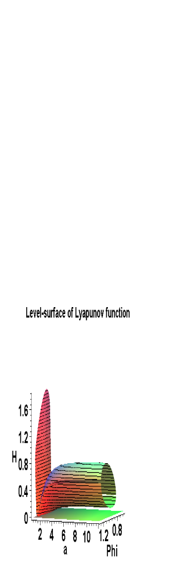
Figure 1:   Level surface of the Lyapunov function $\eta$ (102) for the potential $V(\Phi)$ (73) in presence of radiation and $k=+1$.          

One can see two main specific parts of this quite complicated surface:

1) A high “vertical” part at small values of the RW scale factor $a$. We shall see that the solutions that go into the inner part of the $\{a,\Phi,H\}$-space through this part of the surface describe the regime of inflation of the Universe.

2) An infinitely long “horizontal” tube along the $a$-axes. The solutions that enter the inner part of the $\{a,\Phi,H\}$-space through this part of surface go to de Sitter asymptotic regime winding around the axis of the tube and approaching it for $t\to\infty$.

The behavior of the solutions in these completely different regimes, and the transition of given solution from inflation to asymptotically de Sitter regime will be described in Section VI. C in more detail.

Second Normal Form of the Dynamical Equations

We need one more normal form of the dynamical equations to study the behavior of their solutions for $x_{1},x_{2}\to\infty$. The standard techniques for investigation of the solutions in this limit Arnold show that the infinite point is a complex singular point, and one has to use the so called $\sigma$-process to split this singular point into elementary ones. This dictates the following change of variables:

$$x_{1}={\frac{3}{16}}p_{{}_{\Phi}}^{-2}z^{-4}g^{-4},\,\,\,x_{2}=g^{-1},\,\,\,t={\frac{4}{\sqrt{3}}}\,p_{{}_{\Phi}}\Theta\,,$$ (105)

which transforms the equations (99) with right hand sides (100) into a new system:

$$g^{\prime}=g\,{\cal D},\,\,\,z^{\prime}=z{\cal Z},\,\,\,\Theta^{\prime}=z^{2}g^{2}$$ (106)

where

$${\cal D}(g,z,a;p_{{}_{\Phi}}^{2},k) = 1-{\frac{1}{3}}z^{4}g^{5}w(g)$$

$$- \left(\!{\frac{4p_{{}_{\Phi}}}{3}}\!\right)^{\!2}\!\!g^{3}z^{4}\!\left(\!1\!+\!g^{2}\epsilon(a)\!-\!3g{\frac{k}{a^{2}}}\!\right)\!$$

$$= {\cal D}_{0}(g,z)\!+\!{\cal O}_{2}(p_{{}_{\Phi}}^{2})$$

$${\cal Z}(g,z,a;p_{{}_{\Phi}}^{2},k) = {\frac{1}{4}}z^{4}g^{7}v{,_{g}}(g)$$ (107)

$$+ \left(\!{\frac{4p_{{}_{\Phi}}}{3}}\!\right)^{\!2}\!g^{4}z^{4}\!\left(\!g\epsilon(a)\!-\!{\frac{3}{2}}{\frac{k}{a^{2}}}\!\right)\!$$

$$= \!{\cal Z}_{0}(g,z)\!+\!{\cal O}_{2}(p_{{}_{\Phi}}^{2})\,.$$

Here we have introduced the functions $v(g)\!=\!{\frac{16}{3}}p_{{}_{\Phi}}^{2}\!V({\frac{1}{g}})$ and $w(g)\!=\!{\frac{16}{3}}p_{{}_{\Phi}}^{2}\!W({\frac{1}{g}})$ which do not depend on the parameter $p_{{}_{\Phi}}$ and are simply related: $w=3/2g^{-2}\int_{1}^{g}g^{3}dv$. The functions ${\cal D}$ and ${\cal Z}$ are defined according to formulae

$${\cal D}={\frac{d(\ln g)}{d(\ln a)}}\,,\quad{\cal Z}={\frac{d(\ln z)}{d(\ln a)}}\,.$$ (108)

The representation (107) shows that one can develop a simple perturbation theory for the highly nonlinear system (106) using the extremely small parameter $p_{{}_{\Phi}}^{2}$ as a perturbation parameter.

It is interesting to emphasize that in the domain $a\!\gg\!p_{{}_{\Phi}}^{2/{\bf n}}$ one can consider both the space-curvature term ${\frac{k}{a^{2}}}$ and the matter density $\epsilon(a)$ as small perturbations. Here ${\bf n}=\max\{2,n_{max}\}$ and $n_{max}$ is the largest degree in formula (86). Thus, 4D-DG gives an immediate contribution to the solution of the so-called flatness problem in cosmology. Without further tuning of the model and for any admissible cosmological potential, it becomes clear that at the epoch with $a\sim 1$ the curvature term can be neglected because of the extremely small factor $p_{{}_{\Phi}}^{2}\lesssim 10^{-60}$ in (107). At such epoch, the influence of the matter on the dynamics of the gravi-dilaton sector is negligible as well because of the same reason. Only at very early stages of the evolution of the Universe these terms may have had a significant impact on the gravy-dilaton sector and on the space-time curvature, according to the basic relation (46). In a later epoch, the Universe will look spatially flat if some space-curvature is not accumulated during the Beginning.

From the dynamical equations (99), (100) and (106), one easily obtains the following contour-integral representation for the number of e-folds ${\cal N}$ and for the elapsed time $\Delta t_{\cal N}={\frac{4}{\sqrt{3}}}\,p_{{}_{\Phi}}\Theta_{\cal N}$:

$${\cal N}(p_{{}_{\Phi}}^{2},k)\!=\!\int_{\tau_{in}}^{\tau_{fin}}\limits H^{2}(\tau)d\tau\!=\!\!\int_{{\cal C}_{in}^{fin}}\limits\!{\frac{dg/g}{{\cal D}(g,z,a;p_{{}_{\Phi}}^{2},k)}},$$ (109)

and

$$\Theta_{\cal{}_{N}}(p_{{}_{\Phi}}^{2},k)=\int_{{\cal C}_{in}^{fin}}\limits\!{\frac{z^{2}g\,dg}{{\cal D}(g,z,a;p_{{}_{\Phi}}^{2},k)}}.$$ (110)

Here, a start from some initial (in) state of the 3D-DG-RW Universe, followed by a motion on a contour ${\cal C}_{in}^{fin}$ (determined by corresponding solution of system (106)), and an end at some final (fin) state, are assumed.

VI.3 General Properties of the Solutions in the 4D-DG RW Universe

VI.3.1 Properties of the Solutions in a Vicinity of dSV

Let us first consider the simplest case when $k=0$ and $\epsilon=0$. The system (99) in this case splits into a single equation for $x_{3}$, which is solved by the monotonic function $x_{3}(\tau)=x_{3}^{0}+\int_{\tau_{0}}^{\tau}x_{1}(\tau)d\tau$, and the independent of $x_{3}$ system

$${\frac{d}{d\tau}}{x_{1}}=4x_{1}\left(Z_{1}(x_{2})-x_{1}\right),$$

$${\frac{d}{d\tau}}{x_{2}}=\,\,x_{2}\left(Z_{2}(x_{2})-x_{1}\right).\hskip 0.0pt$$ (111)

Now it is clear that the curves $\hat{x}_{1}=Z_{1}(\hat{x}_{2})$ and $\check{x}_{1}=Z_{2}(\check{x}_{2})$ are the zero-isoclinic lines for the solutions of (111). These curves describe the points of local extrema of the functions $x_{1}(\tau)$ and $x_{2}(\tau)$, respectively, in the domain $x_{1,2}>0$. Because of the condition $U(\Phi)>0$ and the existence of a unique minimum of the cosmological potential (see Propositions 1 and 2), these lines have a unique intersection point – a dSV state with $\bar{x}_{1}=1/3$, $\bar{x}_{2}=1$. This singular point represents the standard de Sitter solution, which in usual variables reads

$$\bar{H}=1/\sqrt{3},\,\,\,\bar{\Phi}=1,\,\,\,a(t)=a_{0}\exp(t/\sqrt{3}).$$ (112)

One can see the typical behavior of the solutions of the system (111) in the domain $x_{1,2}>0$, together with the curves $Z[1]:=\{\hat{x}_{1}=Z_{1}(\hat{x}_{2})\}$, and $Z[2]:=\{\check{x}_{1}=Z_{2}(\check{x}_{2})\}$, in Fig.2, where the corresponding phase portrait is shown for the case of the potentials (73) and $p_{{}_{\Phi}}=1/4$.

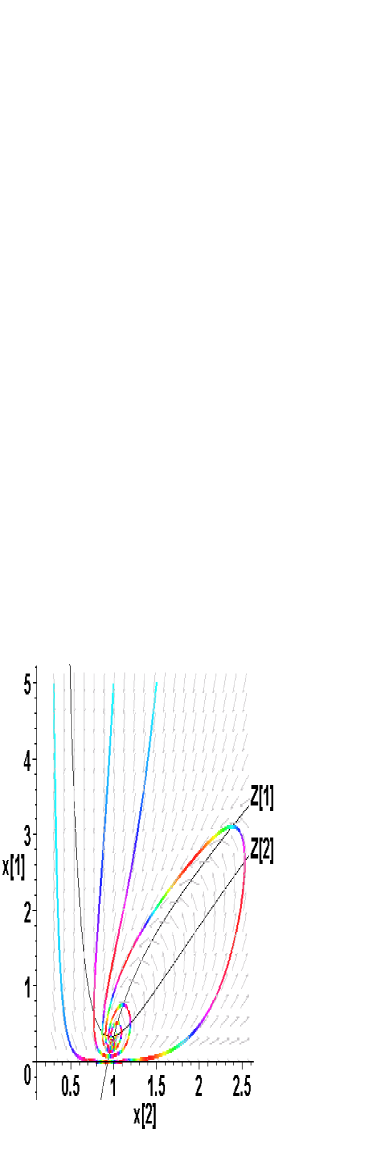
Figure 2:   A typical phase portrait of the system (111). The parts of solutions with the same color are covered by the Universe for equal $\tau$-intervals.          

Consider the solutions of the system (111) of the form $x_{1,2}(\tau)=\bar{x}_{1,2}+\delta x_{1,2}(\tau)$ that are close to dSV, i.e., with $|\delta x_{1,2}(\tau)|\ll 1$. Using the relations (75), one obtains in linear approximation

$$\delta x_{1}(t)=\delta x_{1}^{0}\,\exp\!\left({-{\frac{\sqrt{3}}{2}}t}\right)\cos\left(\omega_{{}_{\Phi}}t\right),\hskip 39.83368pt$$

$$\delta x_{2}(t)\!=\!{\frac{3}{2}}{\frac{p_{{}_{\Phi}}\delta x_{1}^{0}}{\sqrt{p_{{}_{\Phi}}^{2}\!+\!{\frac{3}{4}}}}}\exp\!\left(\!{-{\frac{\sqrt{3}}{2}}t}\!\right)\!\cos\left(\omega_{{}_{\Phi}}t\!-\!\psi_{{}_{\Phi}}\right)$$

$$\delta x_{3}(t)\!=\!\delta x_{3}^{0}\!+\!\sqrt{3}p_{{}_{\Phi}}\delta x_{1}^{0}\exp\!\left(\!{-{\frac{\sqrt{3}}{2}}t}\!\right)\!\times\hskip 34.14322pt$$

$$\bigl{(}\cos\left(\omega_{{}_{\Phi}}t\!-\!\psi_{a}\right)-\cos\left(\psi_{a}\right)\bigr{)}\,,$$ (113)

where

$$\omega_{{}_{\Phi}}=\sqrt{p_{{}_{\Phi}}^{-2}-3/4}\,,\hskip 42.67912pt$$

$$\tan\psi_{{}_{\Phi}}={\frac{2\sqrt{3}}{5}}\,\omega_{{}_{\Phi}},\,\,\,\tan\psi_{a}=-{\frac{2\sqrt{3}}{3}}\,\omega_{{}_{\Phi}},$$ (114)

$\delta x_{1}^{0}=\delta x_{1}(0)$ is the small initial amplitude of $\delta x_{1}(t)$, and the solution for the deviation $\delta x_{3}(t)$ has been added for completeness and for later use.

The frequency $\omega_{{}_{\Phi}}$ is a real and positive number if $p_{{}_{\Phi}}<2/\sqrt{3}$. According to the estimate (82), in 4D-DG we have $\omega_{{}_{\Phi}}\geq 10^{30}$ in cosmological units, or $\omega_{{}_{\Phi}}\geq 10^{3}\,{\rm GHz}$ in usual units, and $\psi_{{}_{\Phi}}\approx\pi/2\approx-\psi_{a}$.

Thus, we see that dSV is a stable focus in the phase portrait of the system (111). For $k=0$ and $\epsilon=0$, all solutions of this system that lie in a small enough vicinity of dSV oscillate with an ultra-high frequency $\omega_{{}_{\Phi}}$ (114), and approach dSV in the limit $t\to\infty$.

Now we generalize this statement for the case of arbitrary $k=0,\pm 1$ and $\epsilon\neq 0$.

Proposition 3: The de Sitter solution $(\ref{dSS})$ is an attractor in the 4D-DG-RW Universe if for $a\to\infty$ we have $\epsilon(a)\sim a^{-n}$ with $n>3/2$. In this case, all solutions that are in a small enough vicinity of the de Sitter solution tend to that solution in the limit $t\to\infty$, oscillating with an ultra-high frequency $(\ref{omega})$. All solutions with an arbitrary $k=0,\pm 1$, and an arbitrary $\epsilon$ have the asymptote $x_{1}(t)\sim{\frac{1}{3}}+\delta x_{1}(t)$, $x_{2}(t)\sim 1+\delta x_{2}(t)$, and $x_{3}(t)\sim x_{3}^{0}+t/\sqrt{3}+\delta x_{3}(t)$, with the same functions $\delta x_{1,2,3}(t)$ $(\ref{dxt})$. In general, the constants $\delta x_{1,3}^{0}$ may depend on $k$ and $\epsilon$.

This turns out to be possible even in the presence of 3-space-curvature and energy-density terms, because in the limit $t\to\infty$ we have $x_{3}\to\infty$, $ke^{-x_{3}}\to 0$ for all $k\!=\!0,\pm 1$ and $\epsilon\!\to\!0$ fast enough, according to formula (86). One can find the proof of this result in Appendix A.

We see that one important general prediction for the 4D-DG-RW Universe is the existence of ultra-high dilatonic oscillations with frequency $\omega_{\Phi}$ (114) in 3-spaces with any curvature and in the presence of any kind of normal matter.

If $p_{{}_{\Phi}}\geq 2/\sqrt{3}$, i.e., if $m_{{}_{\Phi}}\leq 10^{-33}\,{\rm eV}$ (as in inflation models with a slow-rolling scalar field and in quintessence models), the above ultra-high dilatonic oscillations do not exist in the 4D-DG-RW Universe. In this case, the frequency $\omega_{{}_{\Phi}}$ becomes imaginary and, instead of a stable focus, we have an unstable saddle point in the phase portrait of the system (111). Such a situation was considered first in Starobinsky80 in a different model of nonlinear gravity based on a quadratic with respect to scalar curvature $R$ Lagrangian (47), but with some additional terms that originate from quantum fluctuations in curved space-time QNLG . These additional terms vanish in the case of RW metric but yield an essentially different theory in other cases. Therefore, for RW Universe the model described in Starobinsky80 is equivalent to 4D-DG with the non-physical quadratic cosmological potential (72).

An immediate consequence of Proposition 3 is the existence of ultra-high frequency oscillations of the effective gravitational factor $G_{eff}=G_{{}_{N}}/\Phi$, accompanied with an extremely slow exponential decrease of its amplitude $\sim\exp\left(-{\frac{1}{2}}\sqrt{3\Lambda^{obs}}\,ct\right)$ (in usual units). From Eq. (51), one obtains $\bar{H}^{2}/H^{2}_{0}=\Omega_{\Lambda}$ and $\delta H^{2}_{0}={\frac{1}{3}}{\frac{1-\Omega_{\Lambda}}{\Omega_{\Lambda}}}$. Hence, at the present epoch with $\Omega_{\Lambda}\approx{\frac{2}{3}}$, we have $\delta x_{1}^{0}\approx{\frac{1}{6}}$. Then the second equation of the system (113) gives

$$g(t)\approx 1-p_{{}_{\Phi}}{\frac{\sqrt{3}}{2}}\exp\!\left({-{\frac{\sqrt{3}}{2}}t}\right)\cos\left(\omega_{{}_{\Phi}}t-\psi_{{}_{\Phi}}\right)\,,$$ (115)

where we have introduced a dimensionless gravitational factor, $g(t)={{G_{eff}(t)}/{G_{{}_{N}}}}=1/\Phi(t)$.

Because of the extremely small amplitude $\!p_{{}_{\Phi}}\!\leq\!10^{-30}$, these variations are beyond the possibilities of present-day experimental techniques (see Section III. C.).

In contrast, the oscillations of the Hubble parameter $H$ have a relatively big amplitude $\delta H_{0}=\sqrt{\delta x_{0}}\approx 0.4$, and the same huge frequency $\omega_{{}_{\Phi}}$, as the oscillations of gravitational factor. It is very interesting to find possible observational consequences of such phenomena.

High frequency oscillations of the effective gravitational factor were considered first in the context of Brans-Dicke field with BD parameter $\omega>1$ in Steinhardt . These oscillations were induced by an independent inflation field, but the analysis of the existing astrophysical and cosmological limits on the oscillations of $G_{eff}(t)$ is applicable for our 4D-DG model as well. The conclusion in Steinhardt is that the oscillations in the considered frequency-amplitude range, being proportional to $\dot{g}/(gH)$, do not affect the Earth-surface laboratory measurements, Solar System gravitational experiments, stellar evolution, nucleosynthesis, but can produce significant cosmological effects because the frequency is too large and the Hubble parameter is small (in usual units). It can be seen explicitly from Eq. (113) that this is precisely what happens in 4D-DG, although in it the oscillations are self-induced.

As stressed in Steinhardt , despite the fact that the variations of the type (115) have extremely small amplitudes, they can produce significant cosmological effects because of the nonlinear character of gravity. The 4D-DG version of the corresponding formula – analogous to the one in the first of references Steinhardt – is

$$H={\frac{1}{2}}{\frac{\dot{g}}{g}}\pm\sqrt{{\frac{1}{4}}\left({\frac{\dot{g}}{g}}\right)^{2}+{\frac{1}{3}}g(U+\epsilon)-{\frac{k}{a^{2}}}}\,.$$ (116)

Being a direct consequence of Eq. (89), this formula shows that, after averaging of the oscillations, the term ${{\dot{g}}/g}$ has a non-vanishing contribution because it enters the Hubble parameter (116) in a nonlinear manner. A more detailed mathematical treatment of this new phenomenon in 4D-DG is needed to derive reliable conclusions. The standard averaging techniques for differential equations with fast oscillating solutions and slowly developing modes seem to be the most natural mathematical method for this purpose, but the applications of these techniques to 4D-DG lies beyond the scope of the present article.

VI.3.2 Inflation in 4D-DG-RW Universe

Having in mind that: 1) the essence of inflation is a fast and huge re-scaling of Universe, and 2) the dilaton is the scalar field responsible for the scales in Universe, it seems natural to relate these two fundamental physical notions instead of inventing some specific “inflation field”. In this section we show that our 4D-DG model indeed offers such a possibility.

The Phase-Space Domain of Inflation

As seen from the phase portraits in Fig. 2–3, for values $H\geq H_{crit}$ and $\Phi\geq\Phi_{crit}$, the ultra-high-frequency-oscillations do not exist. The evolution of the Universe in this domain of phase space of the system (89) reduces to some kind of monotonic expansion, according to the equation ${\frac{d}{d\tau}}x_{3}=H^{2}>0$. We call this expansion an inflation. As we shall see, it indeed has all needed properties to be considered as an inflation phenomenon inflation .

The transition from inflation to high-frequency oscillations is a nonlinear phenomenon, and we will describe it in the present article very approximately. Here our goal is to have some approximate criteria for determining the end of the inflation. It is needed for evaluation of the basic quantities that describe the inflation.

As seen from Eq. (113), the amplitude, $\delta\Phi_{0}$, of the oscillations of $\Phi$ is extremely small compared with the amplitude $\delta H^{2}$ of the oscillations of $H^{2}$:   $\delta\Phi_{0}\lesssim{\frac{3}{2}}p_{{}_{\Phi}}/\sqrt{p_{{}_{\Phi}}^{2}+{\frac{3}{4}}}\,\delta H_{0}^{2}$. An obvious crude estimate for the amplitude $\delta H_{0}^{2}$ is $\delta H_{0}^{2}\leq 1/3\,(=\bar{H}^{2})$. Then, for $p_{{}_{\Phi}}\leq 2/\sqrt{3}$ (which is the condition for existence of oscillations), we obtain $\delta\Phi_{0}\lesssim\delta H_{0}^{2}\lesssim 1/3$. The last estimate is indeed very crude for the physical model at hand, in which $p_{{}_{\Phi}}\leq 10^{-30}$. This consideration gives the constraint $H_{crit}\lesssim\sqrt{2/3}$ and $\Phi_{crit}\lesssim 4/3$, but, taking into account the extremely small value of $p_{{}_{\Phi}}$, we will use for simplicity the very crude estimate $H_{crit},\Phi_{crit}\sim 1$.

Now it becomes clear that the study of the inflation requires to consider big values of the variables $x_{1,2}$, i.e., to use the second normal form (106) of the dynamical equations.

The Case $k=0$, $\epsilon=0$

Let us consider first the case $k=0$, $\epsilon=0$. From Eq. (106) one obtains the simple first order equation

$${\frac{dz}{dg}}={\frac{z^{5}g^{6}}{4}}{\frac{v_{,_{g}}(g)}{{\cal D}(g,z;p_{{}_{\Phi}}^{2})}}$$ (117)

with

$${\cal D}(g,z;p_{{}_{\Phi}}^{2})=1-{\frac{1}{3}}z^{4}g^{5}u(g)=\hskip 85.35826pt$$

$$1\!-\!{\frac{1}{3}}z^{4}g^{5}w(g)\!-\!\left(\!{\frac{4p_{{}_{\Phi}}}{3}}\!\right)^{\!2}\!\!g^{3}z^{4}\!=\!{\cal D}_{0}(g,z)\!+\!{\cal O}_{2}(p_{{}_{\Phi}}^{2}),\,\,\,\,$$ (118)

where $u(g)={\frac{16}{3}}p_{{}_{\Phi}}^{2}U(1/g)$.

Some basic properties of the solutions of Eq. (117) are derived in Appendix B. It turns out that, for all solutions in the case $k=0$, $\epsilon=0$, there is a Beginning, defined as a time instant $t=0$ at which RW scale factor vanishes, $a(0)=0$, as in GR. In a small vicinity of the Beginning, for the potentials (74), one obtains a different behavior of the solutions, depending on the parameter $\nu_{+}>0$ (see Appendix B).

For $0<\nu_{+}<6$, we have:

$$a(t)\sim\left({\frac{t}{p_{{}_{\Phi}}}}\right)^{1/2}\!\!,\,\,\,g(t)={\frac{1}{z_{0}}}\left({\frac{\sqrt{3}}{4p_{{}_{\Phi}}}}t\right)^{1/2}\!\!+{\cal O}_{3/2}(t),$$

$$z(t)\!=\!z_{0}\!-\!{\frac{4z_{0}^{\nu_{+}-1}\left(\!{\frac{\sqrt{3}}{4p_{{}_{\Phi}}}}t\!\right)^{3\!-\!\nu_{+}/2}}{3(\nu_{+}\!+\!\nu_{-})(6\!-\!\nu_{+})}}\!+\!{\cal O}_{4\!-\!\nu_{+}/2}(t).\,\,\,$$ (119)

Since the behavior of the RW scale factor $a(t)$ for small $t$ is similar to its behavior in GR in the presence of radiation, one can conclude that, if $0<\nu_{+}<6$, at the Beginning the dilaton plays a role, similar to the role of radiation.

For $6\leq\nu_{+}$, we obtain

$$a(t)\sim\left({\frac{t}{p_{{}_{\Phi}}}}\right)^{\alpha}\!\!,\,\,\,g(t)=\left({\frac{\sqrt{3}}{4\alpha z_{1}^{2}p_{{}_{\Phi}}}}t\right)^{\alpha}\!\!+{\cal O}_{\alpha\!+\!1}(t)\!\!,$$

$$z(t)={\rm const}\left(\!{\frac{t}{p_{{}_{\Phi}}}}\!\right)^{\gamma}\!\!+{\cal O}_{\gamma\!+\!1}(t),\hskip 56.9055pt$$

$$\alpha\!=\!{\frac{1}{\nu_{+}-1}}\!\in\!\left(0,{1/5}\right],\,\,\gamma\!=\!{\frac{\nu_{+}-3}{2(\nu_{+}-1)}}\!\in\!\left[3/10,1/2\right).\,\,$$ (120)

For all potentials (74) in 4D-DG, we have zero gravity at the Beginning, i.e., $g(0)=0$. This leads to some sort of an initial power-law expansion, which for $\nu_{+}\geq 6$ is stronger then in GR. The number of e-folds ${\cal N}(t)\to-\infty$ as $t\to+0$ like $\ln t$, since ${\cal N}(t)=\ln a(t)$. For fixed initial time instant $t_{in}>0$, final time instant $t_{fin}>t_{in}$, and number ${\cal N}$, one obtains for the duration of this expansion $\Delta t_{infl}=t_{fin}(1-\alpha/{\cal N})=t_{in}({\cal N}/\alpha-1)$. Hence, the smaller $\alpha$, the faster the initial (hyper)inflation.

The general conclusion is that the potentials (74) do not help to overcome the initial singularity problem in the 4D-DG-RW Universe with $k=0$ and $\epsilon=0$. However, we would like to emphasize that 4D-DG is not applicable for times smaller then the Planck time $t_{Pl}\sim 10^{-44}\,{\rm sec}$, because it is a low-energy theory and ignores quantum corrections in (S)ST. But one can expect 4D-DG to be valid after some initial time instant, $t_{in}\sim t_{{}_{\Phi}}=\hbar/(m_{{}_{\Phi}}c^{2})$. If $m_{{}_{\Phi}}\ll M_{Pl}$, we will have $t_{in}\gg t_{Pl}$ and our results for the case under consideration may have a physical meaning, leaving open the initial singularity problem.

As seen from Eq. (109) and Eq. (107), one can represent the RW scale factor $a(t)$ in the form:

$$a(t)=g(t)\exp(\Delta{\cal N}(t)),$$ (121)

where the re-normalized number of e-folds:

$$\Delta{\cal N}=\int_{{\cal C}_{in}^{fin}}\limits\!{\frac{dg}{g}}\,{\frac{1-{\cal D}(g,z,a;p_{{}_{\Phi}}^{2},k)}{{\cal D}(g,z,a;p_{{}_{\Phi}}^{2},k)}}$$ (122)

is a finite quantity in the entire time interval $t\in[0,\infty)$. Obviously, $\Delta{\cal N}(t^{(i)})\equiv{\cal N}(t^{(i)})$ at the special time instants $t^{(i)}$, $i=0,1,...$, when $g(t)$ reaches its dSV value, i.e., when $g(t^{(i)})=1$, for example, in the limit $t\to\infty$.

The phase portrait of Eq. (117) and the time-dependence of the dimensionless gravitational factor $g(t)$ for the potentials (73) are shown in Fig. 3 and Fig. 4, respectively. From Fig. 4 we see that one can define analytically the time of duration of the initial inflation $\Delta t_{infl}^{(0)}$ as the time spent by Universe from the Beginning to the first time instant $t^{(0)}$, when the gravitational factor $g(t^{(0)})=1$. In addition, we see in Fig. 4 that this time interval is finite and has different values for different solutions of Eq. (117).

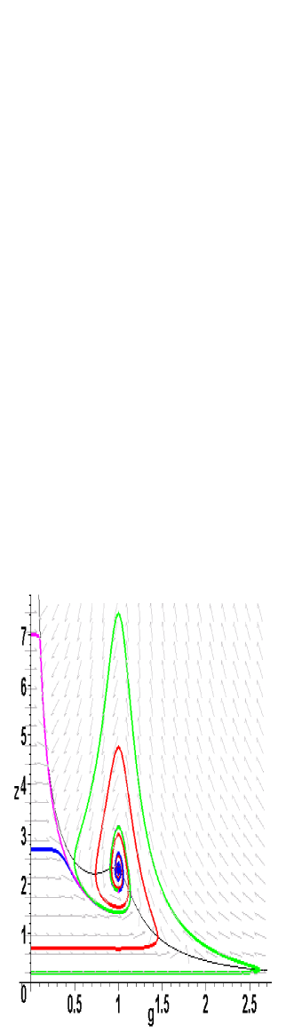
Figure 3:   The phase portrait of Eq. (117). The black line shows the zero line Z[2] of the denominator ${\cal D}$.          

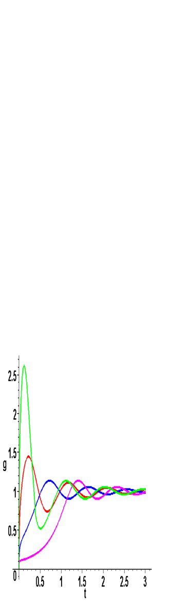
Figure 4:   The dependence of dimensionless gravitational factor g on cosmic time t for solutions of Eq. (117).          

In Fig. 2 and Fig. 3 one can see a new specific feature of 4D-DG: the solutions may enter many times the phase-space domain of inflation and the function $g(t)$ oscillates around its dSV value $\bar{g}=1$ with a variable preriod. Between two successive maxima of $g(t)$, the squared logarithmic derivative $H^{2}$ of $a(t)$ has its own maxima, just at the already defined time instants $t^{(i)}$. In the vicinity of each maximum of $H^{2}$, the function a(t) increases very fast – like $\exp({\rm const}\times t^{\aleph})$, with ${\rm const}>0$, and parameter $\aleph\geq 2$. Therefore, we call such inflation, which is much faster than the usual exponential de Sitter inflation, a hyper-inflation. Hence, in 4D-DG, we have some sort of successive hyper-inflations in the Universe. For simplicity, we define the time-duration $\Delta t_{infl}^{(i)}=t^{(i)}-t^{(i-1)}$, $i=0,1,...$ (by definition $\Delta t_{infl}^{(0)}=t^{(0)}$) of each of these periods of hyper-inflation as the time period between two successive dSV values of the function $g(t)$, although the hyper-inflation itself takes place only around the maxima of the function $H^{2}(t)$. The corresponding number of e-folds is ${\cal N}_{infl}^{(i)}$. It is clear that ${\cal N}_{infl}^{(i)}$ is a decreasing function of the number $i$. The inflation can be considered as cosmologically significant only if for some short total time period $\Delta t_{infl}^{total}=\sum_{i=0}^{i_{max}}\Delta t_{infl}^{(i)}$, the total number of e-folds ${\cal N}_{infl}^{total}=\sum_{i=0}^{i_{max}}{\cal N}_{infl}^{(i)}$ exceeds some large enough number ${\cal N}$. It is known that one needs to have ${\cal N}\gtrsim 60$ to be able to explain the special-flatness problem, the horizon problem, and the large-scales-smoothness problem in cosmology C .

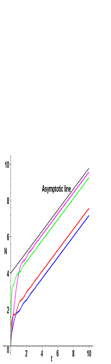
Figure 5:   The dependence of the number of e-folds ${\cal N}$ on the cosmic time $t$ for solutions of Eq. (117). The straight black line gives an example of an asymptotic line for some solution.          

Fig. 5 illustrates both the inflation and the asymptotic behavior of the function ${\cal N}(t)$ for $t\to\infty$. The small oscillations of this function are “averaged” by the crude graphical abilities of the drawing device, and for large values of time $t$ we actually can see in Fig. 5 only the limiting de Sitter regime (112), when the averaged finction $\langle{\cal N}(t)\rangle\equiv\langle\Delta{\cal N}(t)\rangle$. In this regime, for $t\to\infty$, we have an obvious asymptotic of the form  $\langle{\cal N}(t)\rangle\sim\bar{\cal N}+\bar{H}t$ for the averaged with respect to dilatonic oscillation (113) function $\langle{\cal N}(t)\rangle$. We accept the constant $\bar{\cal N}$ as our final definition of total number of e-folds during inflation:

$$\bar{\cal N}=\lim_{t\to\infty}\left(\langle{\cal N}(t)\rangle-\bar{H}t\right)=\lim_{t\to\infty}\left(\langle\Delta{\cal N}(t)\rangle-\bar{H}t\right).\,\,$$ (123)

It is clear that this integral characteristic describes precisely the number of e-folds due to the true inflation in 4D-DG, i.e., during the fast initial expansion of the Universe, as a new physical phenomenon. To obtain this quantity, one obviously must subtract the asymptotic de Sitter expansion from the total function $\langle{\cal N}(t)\rangle$. According to Proposition 3, one can apply the same definition for solutions in the general case of arbitrary values of the space-curvature parameter $k$ and physically admissible energy densities $\epsilon(a)$ since they have the same asymptotic. Hence, in all cases the solutions with a cosmologically significant inflation must have values $\bar{\cal N}\gtrsim 60$.

As we see in Fig. 5, the total number of e-folds $\bar{\cal N}$ decreases, starting from the ’green” solution (with $z_{0}=0.2$) to the “red” one (with $z_{0}=0.7$) and to the “blue” one (with $z_{0}=2.7$), reaches a minimum ($\approx 1$) for some initial value $z_{0}^{*}$, and then increases for the “magenta” solution (with $z_{0}=7$), and for solutions with larger values of $z_{0}$. Thus, we see that inflation is a typical behavior for all solutions of Eq. (117), and that most of them have large values of $\bar{\cal N}$. (In Fig. 5, we show only solutions with small values of $\bar{\cal N}$ that are close to its minima.)

The value of the constant $\bar{\cal N}$ depends on the closeness of the given solution to the zero curve $Z[2]$ of the denominator of the integrand in the right-hand side of (110). The equation ${\cal D}=0$ can be explicitly solved. Its solution reads $z=\left({\frac{1}{3}}g^{5}u(g)\right)^{-1/4}$. The corresponding curve is shown both in Fig. 2 and Fig. 3.

The value of the quantity ${\cal N}(t)$ increases essentially each time when the solution approaches this curve. The corresponding increment of ${\cal N}(t)$ remains finite, even if the solution crosses this curve, although in this case the denominator in the integrals (109), or (122), reaches a zero value (see Appendix B). Hence, an essential increase in ${\cal N}(t)$ is accumulated when the solution becomes close and parallel to the curve $Z[2]$. This is possible both for big values of $g$ and small values of $z$ (the “green” solution), or for small values of $g$ and big values of $z$ (the “magenta” solution). All this results in a big value of $\bar{\cal N}$. Only a small fraction of the solutions (like the “blue” one and “red” one) stay all the time relatively far from the line ${\cal D}=0$, and therefore acquire relatively small number of e-folds, $1\lesssim\bar{\cal N}\lesssim 2$.

This qualitative consideration, combined with the structure of the phase portrait shown in Figures 2 and 3, not only explains the universal character of the inflation in 4D-DG, but gives us a better understanding of its basic characteristics. Hence, we do not need fine tuning of the model to describe the inflation as a typical physical phenomenon.

Using Eqs. (109), (110), and (118), we obtain

$${\cal N}_{infl}^{(i)}(p_{{}_{\Phi}}^{2})={\cal N}_{infl}^{(i)}(0)+{\cal O}_{2}(p_{{}_{\Phi}}),\hskip 5.69046pt$$

$$t_{infl}^{(i)}(p_{{}_{\Phi}}^{2})={\frac{4}{\sqrt{3}}}p_{{}_{\Phi}}\Theta_{infl}^{(i)}(0)+{\cal O}_{3}(p_{{}_{\Phi}}),$$

where

$${\cal N}_{infl}^{(i)}(0)=\int_{{\cal C}_{in}^{fin}(i)}\limits{\frac{dg/g}{{\cal D}(g,z;0)}},\,\,\,\hbox{and}$$

$$\Theta_{infl}^{(i)}(0)=\int_{{\cal C}_{in}^{fin}(i)}\limits{\frac{z^{2}g\,dg}{{\cal D}(g,z;0)}},\hskip 4.26773pt$$ (124)

are independent of the parameter $p_{{}_{\Phi}}$. Taking into account the extremely small physical value of this parameter, one can conclude that the higher order terms in ${\cal N}_{infl}^{(i)}(p_{{}_{\Phi}}^{2})$ and $\Delta t_{infl}^{(i)}(p_{{}_{\Phi}}^{2})$ are not essential. Neglecting them, we actually ignore the contribution of the term $\Phi/3$ in the functions $Z_{1,2}$ (101), or the corresponding term $\Phi^{2}$, in the cosmological potentials $U(\Phi)$ (61), (73), (74). It is natural to ignore these terms in the domain of inflation, because they are essential only in a small vicinity of dSV. In the function $W(\Phi)$, we have a term that dominates for $\Phi-1\gg p_{{}_{\Phi}}^{2}$, having a huge coefficient $\sim p_{{}_{\Phi}}^{-2}$. Physically this approximation means that we are neglecting the small pure cosmological constant term in the cosmological potential and preserve only the terms, which are proportional to the mass of dilaton.

The relation $\Delta t_{infl}^{(i)}(p_{{}_{\Phi}}^{2})\sim{\frac{4}{\sqrt{3}}}p_{{}_{\Phi}}\Theta_{infl}^{(i)}$, written in physical units, reads

$$E_{{}_{\Phi}}\Delta t_{infl}^{(i)}\sim\hbar{\frac{4}{\sqrt{3}}}\Theta_{\cal N}^{(i)}(0).$$ (125)

It resembles some kind of a quantum “uncertainty relation” for the rest energy $E_{{}_{\Phi}}$ of the dilaton and the time of inflation and maybe indicates the quantum character of the inflation as a physical phenomenon.

More important for us is the fact that Eq. (125) shows the relationship between the mass of dilaton, $m_{{}_{\Phi}}$, and the time duration of inflation. Having large enough mass of dilaton, we will have small enough time duration of inflation. This recovers the real meaning of the mass $m_{{}_{\Phi}}$ as a physical parameter in 4D-DG, and gives possibility to determine it from astrophysical observations as a basic cosmological parameter.

The Case $k\neq 0$ and $\epsilon\neq 0$

The nonzero space-curvature term with $k=\pm 1$, and the presence of matter with $\epsilon(a)\neq 0$ of the form (86) change drastically the behavior of the solution for small values of $g$ and $a$. They yield a multitude of new possibilities. Indeed, if one assumes the physically natural value $n_{max}=4$ in Eq. (86), the system of differential equations (106) has to be rewritten in two new forms. The first one, for the case $0<\nu_{+}<6$, is

$${\frac{dg}{d\sigma_{1}}}\!=\!g\!\left(\!{\cal D}_{\nu_{+}\nu_{-}}^{(0,0)}(g,z)a^{4}\!-\!\left(\!{\frac{4p_{{}_{\Phi}}}{3}}\!\right)^{\!2}\!\!g^{4}z^{4}\!\Bigl{(}ga^{4}\epsilon\!-\!3ka^{2}\!\Bigr{)}\!\right),$$

$${\frac{dz}{d\sigma_{1}}}\!=\!z\!\left(\!{\cal Z}_{\nu_{+}\nu_{-}}^{(0,0)}(g,z)a^{4}\!+\!\left(\!{\frac{4p_{{}_{\Phi}}}{3}}\right)^{\!2}\!\!g^{4}z^{4}\!\Bigl{(}\!ga^{4}\epsilon\!-\!{\frac{3}{2}}ka^{2}\!\Bigr{)}\!\right),$$

$${\frac{da}{d\sigma_{1}}}\!=\!a^{5}.\hskip 187.78836pt$$ (126)

If $6<\nu_{+}$, one has to introduce, instead of regularizing parameter $\sigma_{1}$, another one, $\sigma_{2}$, by $d\sigma_{1}=g^{\nu_{+}-6}d\sigma_{2}$, and to rewrite the system (126) in a similar form by multiplying the right hand sides by $g^{\nu_{+}-6}$. Here ${\cal D}_{\nu_{+}\nu_{-}}^{(0,0)}(g,z)$ and ${\cal Z}_{\nu_{+}\nu_{-}}^{(0,0)}(g,z)$ are polynomials in the variables $g$ and $z$, described in Appendix B, and under our assumption that $n_{max}=4$, the expression $a^{4}\epsilon(a)$ is a polynomial in $a$ of degree less than $4$. The canonical polynomial form of the right-hand sides of Eqs. (126), and in the analogous system in the second case, makes transparent the fact that the point $a=0$, $g=0$, $z=0$ is a complex singular point which has a rich structure – different for $0<\nu_{+}<6$ and for $6<\nu_{+}$.

For different initial conditions and different cosmological potentials, one can observe numerically different types of solutions: bouncing ones, oscillating ones, and solutions that are similar to the one we have discussed in the case $k=\epsilon=0$. They have inflation regime and de Sitter asymptotic for $t\to\infty$ (in accordance with Proposition 3).

Hence, in the presence of space-curvature and matter, a novel approach to the initial singularity problem is possible in 4D-DG. The systematic study of properties of solutions of both systems of type (126) which arise for potentials (74) is a complicated mathematical issue and deserves independent investigation.

Static and Turning Points in the Case $k=+1$

In the case $k=+1$, there may exist turning points in the evolution of $a(t)$ with $\dot{a}=0$ and $\ddot{a}=0$, some of them being unstable static solutions, $a(t)\equiv{\rm const}$, similar to the original Einstein static solution in GR with $\Lambda>0$. In the $(\Phi,a)$-plane, these points lie on the line

$$\epsilon_{pot}=U(\Phi)+\epsilon(a)-{{3\Phi}\over{a^{2}}}=0,$$ (127)

which may have a complicated structure depending on $U(\Phi)$ and $\epsilon(a)$. The analytical form of the solutions and the form of the corresponding level surface of the Lyapunov function $\eta$ in a vicinity of this line are interesting from mathematical point of view, but we will not describe them in the present article. In the cases $k=-1$ and $k=0$, such phenomena are not possible in 4D-DG.

VI.4 The Inverse Cosmological Problem in 4D-DG

Instead of representing the system (97) in the normal form (99), we can exclude the cosmological potential $U(\Phi)$, and arrive at a linear differential equation of second order for the function $\Phi(x_{3})$,

$$\Phi^{\prime\prime}\!+\!\left({\frac{H^{\prime}}{H}}\!-\!1\right)\Phi^{\prime}\!+\!2\left({\frac{H^{\prime}}{H}}\!-{\frac{k}{H^{2}}}e^{-2x_{3}}\right)\Phi\!=\!{\frac{\epsilon^{\prime}}{3H^{2}}},\,\,\,\,$$ (128)

equivalent to Eq. (90) because of the relation $\epsilon^{\prime}+3(\epsilon+p)=0$ .

In terms of the function $\psi(a)=\sqrt{|H(a)|/a}\,\Phi(a)$ the equation (128) reads

$$\psi^{\prime\prime}+n^{2}\psi=\delta,$$ (129)

where we have introduced the new functions

$$-n^{2}={\frac{1}{2}}{\frac{H^{\prime\prime}}{H}}-{\frac{1}{4}}\left({\frac{H^{\prime}}{H}}\right)^{2}\!-{\frac{5}{2}}{\frac{H^{\prime}}{H}}+{\frac{1}{4}}+{\frac{2k}{H^{2}}}e^{-2x_{3}},$$

$$\delta={\frac{\epsilon^{\prime}\,e^{-x_{3}/2}}{3\,|H|^{3/2}}}.\hskip 143.6865pt$$ (130)

The Schrödinger-like equation (129) for $\psi(x_{3})$ can be analyzed with some well known mathematical tools. For example, the condition $n(x_{3})<0$ ensures the absence of a new type of oscillations of the field $\Phi(x_{3})=\sqrt{1/|H(x_{3})|}e^{x_{3}/2}\,\psi(x_{3})$ in domains where $H(x_{3})$ is a monotonic function. In the opposite case, $n(x_{3})\!>\!0$, we do have such oscillations – only of the dilaton field $\Phi$ as a function of scale parameter $a=e^{x_{3}}$. This type of dilaton oscillations is different from the one described in Section VI.B.1.

Now we are ready to consider the inverse cosmological problem:

Find the cosmological potential $U(\Phi)$ and the dilatonic potential $V(\Phi)$ that yield a given evolution of the Universe, determined by the function $a(t)$.

It is remarkable that in 4D-DG the following result take place:

Proposition 4: For any three times differentiable function $a(t)$ in 4D-DG, there exist a two-parameter family of local solutions of the inverse cosmological problem.

Indeed, given $a(t)$, we can construct the function $H(x_{3})$ and find the general solution $\Phi(x_{3};\tilde{x}_{3},\tilde{\Phi},\tilde{\Phi}^{\prime})$ of the linear second order differential equation (128) in the following Cauchy form:

$$\Phi(x_{3};\tilde{x}_{3}\tilde{\Phi},\tilde{\Phi}^{\prime})\!=\!C_{1}\Phi_{1}(x_{3})\!+\!C_{2}\Phi_{2}(x_{3})\!+\!\Phi_{\epsilon}(x_{3}).$$ (131)

Here

$$C_{1}=(\tilde{\Phi}_{2}^{\prime}\tilde{\Phi}-\tilde{\Phi}_{2}\tilde{\Phi}^{\prime})/\tilde{\Delta},\,\,\,\,C_{2}=(\tilde{\Phi}_{1}\tilde{\Phi}^{\prime}-\tilde{\Phi}_{1}^{\prime}\tilde{\Phi})/\tilde{\Delta},$$

the functions $\Phi_{1}(x_{3})$ and $\Phi_{2}(x_{3})$ constitute a fundamental system of solutions of the homogeneous equation associated with the non-homogeneous one, (128), (nontrivial examples for such solutions can be found in F00 ),

$$\Delta(x_{3}):=\Phi_{1}\Phi_{2}^{\prime}-\Phi_{2}\Phi_{1}^{\prime}=(\tilde{\Delta}\tilde{H})e^{x_{3}-\tilde{x}_{3}}/H(x_{3})\neq 0,$$

and the term

$$\Phi_{\epsilon}\!=\!{\frac{1}{3\tilde{H}\tilde{\Delta}}}\!\!\left(\!\Phi_{2}\!\int_{\tilde{x}_{3}}^{x_{3}}\limits\!\Phi_{1}{\frac{e^{-(x_{3}-\tilde{x}_{3})}}{H}}d\epsilon-\Phi_{1}\!\int_{\tilde{x}_{3}}^{x_{3}}\limits\!\Phi_{2}{\frac{e^{-(x_{3}-\tilde{x}_{3})}}{H}}d\epsilon\!\right).$$

describes the contribution of matter. The point $\tilde{x}_{3}$ lies in the admissible domain, and $\tilde{\Phi}$ and $\tilde{\Phi}^{\prime}$ are some initial values at $\tilde{x}_{3}$. The tilde sign shows that the corresponding quantities are calculated at the initial point $\tilde{x}_{3}$.

Then, the cosmological potential and the dilatonic potential, as functions of $x_{3}$, are determined by equations

$$U(x_{3};\tilde{\Phi},\tilde{\Phi}^{\prime})\!=\hskip 179.25244pt$$

$$3\Phi(x_{3};\tilde{\Phi},\tilde{\Phi}^{\prime})\left(H^{2}\!+\!ke^{-2x_{3}}\right)\!+\!3H^{2}\Phi^{\prime}(x_{3};\tilde{\Phi},\tilde{\Phi}^{\prime})\!-\!\epsilon,\hskip 0.0pt$$

$$V(x_{3};\tilde{\Phi},\tilde{\Phi}^{\prime})\!={\frac{2}{3}}\Phi(x_{3};\tilde{\Phi},\tilde{\Phi}^{\prime})U(x_{3};\tilde{\Phi},\tilde{\Phi}^{\prime})\!-\hskip 42.67912pt$$

$$\!2\int d\Phi(x_{3};\tilde{\Phi},\tilde{\Phi}^{\prime})U(x_{3};\tilde{\Phi},\tilde{\Phi}^{\prime}),\hskip 34.14322pt$$ (132)

which define the functions $U(\Phi;\tilde{\Phi},\tilde{\Phi}^{\prime})$ and $V(\Phi;\tilde{\Phi},\tilde{\Phi}^{\prime})$ implicitly, i.e., via the inverse function $x_{3}(\Phi;\tilde{\Phi},\tilde{\Phi}^{\prime})$ of the function $\Phi(x_{3};\tilde{\Phi},\tilde{\Phi}^{\prime})$.

Hence, one can construct a two-parameter family of cosmological and dilaton potentials for a given scalar factor $a(t)$. This way, we see that in the 4D-DG-RW model of Universe one can find potentials for which there exist solutions without initial singularities: $a(t_{in})=0$ (which are typical for GR), with any desired kind of inflation, or with other needed properties of RW scale factor $a(t)$. But, in general, one cannot guarantee all necessary properties of these potentials, like the existence of only one minimum, or even the single-valuedness of the functions (132). The sufficient conditions on the function $a(t)$ that which guarantee such properties of the potentials $U$ and $V$ are not known at present.

Here we shall make one more step – to consider the choice of the point $\tilde{x}_{3}$, and of initial values $\tilde{\Phi}$ and $\tilde{\Phi}^{\prime}$. These have to reflect some known basic properties of 4D-DG. So far, the only established general properties of this type are the corresponding values for the unique de Sitter vacuum (75) (see Section IV.C.3).

Proposition 5: In the unique dSV-state of Universe:

$$\bar{x}_{3}=\infty,\hskip 17.07182pt$$

$$\bar{\Phi}=1,\,\,\,\bar{\Phi}^{\prime}=0,$$

$$\bar{H}=1/\sqrt{3},\,\,\,\bar{H}^{\prime}=0,$$

$$\hbox{and}\,\,\,\bar{\Delta}e^{-\bar{x}_{3}}=1.$$ (133)

The corresponding quantities approach these values in the limit $x_{3}\to\infty$.

The proof is based on the following observations:

1) For dSV-state of Universe we have $\epsilon=0$, according to definition (62). Then, from Eq. (86), we see that this unique state corresponds to $\bar{x}_{3}=\infty$. Hence, other quantities for dSV must be considered in the limit $x_{3}\to\infty$. The second of Eq. (86) shows that $\bar{p}=0$, and, together with the conservation of energy-momentum of matter, it leads to the relation $\bar{\epsilon}^{\prime}=0$. (Actually, one can weaken the conditions on the behavior of these quantities simply by requiring that $\bar{\epsilon}=0$ and $\bar{\epsilon}^{\prime}=0$. This is enough for our purposes in this section.)

2) Then, from the above equations, we obtain the values described in Proposition 5:

i) from Eq. (60) – $\bar{\Phi}=1$;

ii) from Eq. (112) – $\bar{H}=1/\sqrt{3}$;

iii) from Proposition 3 and Eq. (113) – $\bar{\Phi}^{\prime}=\bar{H}^{\prime}=0$;

iv) from Eq. (128), which reduces in this limit to $\Phi^{\prime\prime}-\Phi^{\prime}=0$, we see that there exist two fundamental solutions, $\Phi_{1,\infty}(x_{3})\sim 1$ and $\Phi_{2,\infty}(x_{3})\sim e^{x_{3}}(=a)$. Hence, for them $\Delta(x_{3})\sim e^{x_{3}}$ and this proves the last relation in Eq. (133).

As a result of Proposition 5, we obtain the following final form of solution (131):

$$\Phi_{\infty}(x_{3})=\Phi_{1,\infty}(x_{3})+\Phi_{\epsilon,\infty}(x_{3}),$$ (134)

where $\Phi_{1,\infty}(x_{3})$ is the fundamental solution of Eq. (128) that has the asymptotic behavior $\Phi_{1,\infty}(x_{3})\sim 1$ as $x_{3}\to\infty$. Then

$$\Phi_{\epsilon,\infty}\!=\!{\frac{1}{\sqrt{3}}}\!\!\left(\!\Phi_{1}\!\int_{x_{3}}^{\infty}\limits\!\Phi_{2}{\frac{e^{-x_{3}}}{H}}d\epsilon-\Phi_{2}\!\int_{x_{3}}^{\infty}\limits\!\Phi_{1}{\frac{e^{-x_{3}}}{H}}d\epsilon\!\right).$$ (135)

If we wish to reconstruct the cosmological potential $U(\Phi)$ and the dilaton potential $V(\Phi)$ according to relations (132), Eq. (135) requires to know the value of the function $H(x_{3})$ in the future! Of course, if we know the exact dependence of Hubble parameter on $x_{3}$ in the past, we can obtain its values in the future using standard mathematical techniques for analytical continuation. It is interesting to reconsider the available observational data from this point of view, taking into account the theoretical restrictions (133), but this problem lies beyond the scope of the present article.

VII A Novel Adjustment Mechanism for the Cosmological Constant Problem

VII.1 Value of $\Lambda^{obs}$ and Number of Degrees of Freedom in the Observable Universe

Concerning the observed small positive value of the cosmological constant (51), which seems mysterious from point of view of quantum field theory, we see that the real problem one has to solve is to explain the extremely small value $P\approx 10^{-61}$ of Planck number. This number appears not only in the formula (57) for the cosmological constant, but also in the formula (58) for the unit of action and in expression (50) for the action of the gravy-dilaton sector. This observation yields a new possible direction for investigations: one can try to transform the cosmological constant problem to the problem of explaination of the value of the total action in the Universe. It seems natural to think that the huge ratio ${\cal A}/\hbar\sim 10^{122}$ is produced during the long evolution of the Universe in the time interval $\Delta t_{U}\sim 4\times 10^{17}{\rm sec}$. Then the new question is, how many degrees of freedom do we have in the observable Universe, and what is the amount of action accumulated in them since the Beginning.

To answer this question in 4D-DG, we need estimates for the amount of matter action and the action in the gravi-dilaton sector.

1. Amount of action in the matter sector:

We can obtain a crude estimate for the amount of matter action in the observable Universe by using the following purely qualitative analysis PF003 .

First we consider the simplest model of the Universe built only of Bohr hydrogen atoms in ground state, i.e., we describe the whole content of the Universe by using such effective Bohr hydrogen (EBH) atoms. Then for the time of the existence of Universe, $\Delta t_{U}\sim 4\times 10^{17}{\rm sec}$, one EBH atom with Bohr angular velocity $\omega_{B}=m_{e}e^{4}\hbar^{-3}\sim 4\times 10^{16}{\rm sec}^{-1}$ accumulates classical action ${\cal A}_{EBH}=3/2\,\omega_{B}T_{U}\,\hbar\sim 2.4\times 10^{34}\,\hbar$. Hence, the number of EBH in Universe that is needed to explain the value of the present-epoch action ${\cal A}\sim{\cal A}_{c}$, must be $N_{EBH}\sim 5\times 10^{87}$. This seems to be quite a reasonable number, taking into account that the number of barions in observable Universe is $N_{barions}^{obs}\sim 10^{78}$.

Thus, we see that within our “action approach”, when applied to the observed Universe, the discrepancy between the above primitive model and observations is only about $10^{9}$ times. One has to compare this very crude estimate with the corresponding one in quantum field “derivation” of cosmological constant that differs from observation $10^{54}$ – $10^{122}$ times. We have at our disposal some $9$ powers of 10 to solve the problem by taking into account the contribution of all other constituents of matter and radiation (quarks, leptons, gamma quanta, etc.), and the contribution of the gravi-dilaton sector during the evolution of the Universe from the Beginning to the present epoch.

Neglecting the temperature evolution of the Universe during the hot Big Bang phase, we obtain an accumulated action ${\cal A}_{\gamma}\sim\omega_{\gamma}T_{U}\,\hbar\sim 10^{30}\,\hbar$ for one $\gamma$-quantum of CMB (which is the most significant part of present days radiation in Universe).

A simple estimate for the Bohr-like angular velocity of the constituent quarks in a proton is $\omega_{Bq}=m_{e}/m_{q}(r_{B}/r_{p})^{2}\omega_{B}\approx 10^{7}\omega_{B}$ (where the mass of the constituent quark, $m_{q}\sim 5{\rm MeV}$, the standard Bohr radius $r_{B}$ and the known radius of proton $r_{p}\sim 8\times 10^{-13}{\rm cm}$ have been used). Then the action accumulated by the constituent quarks in one proton during the evolution of the Universe is ${\cal A}_{p}\sim\omega_{Bq}T_{U}\,\hbar\sim 10^{42}\,\hbar$. This gives an unexpectedly good estimate for the number of effective protons (ep) in the Universe: $N_{ep}\sim 10^{80}$.

We may use the two remaining orders of magnitude to take into account the contribution of the other matter constituents, of the dark matter (see Primack and the references therein), and of the temperature evolution of Universe – during the short-time initial hot phase, some additional action must be produced in the matter sector.

Using the same arguments in opposite direction (i.e., using them to obtain an estimate of the total action in the matter sector instead of obtaining the number of particles in it), we can say that according to our crude analysis, the amount of action ${\cal A}_{matt}$ accumulated in the matter sector during the evolution of the observable Universe is between $10^{-2}$ and $1$ (in cosmological units).

2) Amount of action in the gravi-dilaton sector:

A similar crude estimate of the amount of action in the gravi-dilaton sector of 4D-DG, based on completely different reasoning, can be derived from formula (50). Unfortunately, at the moment we do not know the form of the solutions in the 4D-DG-RW Universe during the short inflation epoch in the presence of matter. But we know them during the infinite time interval of de Sitter regime – see formulae (113). Ignoring the inflation epoch and the small oscillations of the dilaton $\Phi$ during de Sitter regime (which will be averaged in the integration in expression (50)), we can substitute the simple de Sitter solution (112) in the integral (50). This gives immediately the value $1$ of the integrand, independently of the choice of a cosmological potential $U(\Phi)$ (see (75)). Hence, for the 4D-DG gravi-dilaton action in a unit 3-volume, we obtain in cosmological units ${\cal A}_{g,\Phi}\sim\Delta t_{U}\sim 1$, independently of the choice of a cosmological potential.

If the inflation epoch gives a small additional contribution to both ${\cal A}_{matt}$ and ${\cal A}_{g,\Phi}$, then ${\cal A}_{tot}={\cal A}_{matt}+{\cal A}_{g,\Phi}\sim 1$ (in cosmological units), and we obtain a physical explanation of relation (58) which defines the value of Planck number in this approach. Thus we would have reached an explanation of small value $\Lambda^{obs}=1$ (in cosmological units) in phenomenological frame having explanation of the huge value of the present-epoch-action in Universe.

We see that, in the framework of 4D-DG, the answer to the question, why the cosmological constant is so small in the phenomenological frame, might be: Because the Universe is old and has a huge, but limited, number of degrees of freedom in it. The first part of this answer was proposed in the quintessence models developed in the last decade Q . As we saw, 4D-DG is physically an essentially different model, but it leads to the same conclusion.

In addition, the above consideration gives us some idea how to explain the cosmological coincidence problem when reformulated in terms of action: the actions ${\cal A}_{matt}$ and ${\cal A}_{g,\Phi}$ are of the same order of magnitude, at least in our crude approximation. This result will still hold if the inflation epoch gives comparable contributions to both of actions.

The main conclusion of the above crude arguments is that within the framework of 4D-DG the observed small positive value of the cosmological constant $\Lambda^{obs}$  (51) actually restricts the number of degrees of freedom in the observable Universe. Similar conclusion was reached recently in Fischler by using completely different arguments. Thus, it is possible that a small positive $\Lambda^{obs}$ forbids the existence of a large number of more fundamental levels of matter below the quark level.

It is obvious that these considerations need deeper investigation based on quantum field theory, on the Standard Model, on the modern cosmological results about the evolution of the Universe and the Big Bang. To make them rigorous, one needs to know the detailed description of the 4D-DG inflation in the presence of matter and space-curvature. Another possible scenario is an inflation without matter after dilaton-scale time $t_{{}_{\Phi}}=\hbar/m_{{}_{\Phi}}c^{2}$ (described in Section VI.C), accomplished with some mechanism of creation of matter by gravi-dilaton sector at the end, or after this stage of inflation.

VII.2 A Possible Novel Adjustment Mechanism for $\Lambda$

Here we describe a possibility to solve the cosmological constant problem by employing a novel adjustment mechanism. The basic idea is very simple: one can have a huge cosmological constant in the stringy frame, as a result of vacuum fluctuations of different quantum fields introduced by string theory. In spite of this, the transition to phenomenological frame may reduce the value of this huge constant to the observable one (51) because of the corresponding Weyl transformation (12).

Indeed, taking into account the relations (14), (23), (41), and (42) connecting the SF cosmological potential and the PhF$\equiv$TF one, we obtain

$$\Lambda^{obs}U(\Phi)={}_{{}_{S}\!}\Lambda(\phi)\exp(D{}_{{}_{T}\!}\sigma_{\!{}_{S}}(\phi)).$$ (136)

Hence, to solve the cosmological constant problem, in dS-vacuum state we must have

$${}_{{}_{T}\!}\sigma_{\!{}_{S}}(\bar{\phi})={\frac{1}{D}}\ln\left(\!{\frac{{}_{{}_{S}\!}\Lambda(\bar{\phi})}{\Lambda^{obs}}}\!\right)\!=\!{\frac{1}{D}}\ln P^{-2},\,\,\,$$ (137)

where we have used the normalization (60). For $D=4$ and for the value of Planck number given by (57), we obtain ${}_{{}_{T}\!}\sigma_{\!{}_{S}}(\bar{\phi})\approx 70$. Then, in tree-level approximation (45), we see that one needs vacuum values of the SF dilaton

$$\bar{\phi}\approx 45,\,\,\,\hbox{or}\,\,\,\bar{\phi}\approx 166$$ (138)

to rescale the huge value of ${}_{{}_{S}\!}\Lambda(\bar{\phi})$ in SF to the observed value (51) in PhF$\equiv$TF.

At present, the vacuum value of the SF dilaton $\phi$ is not known as physical quantity, and the above values (138) do not seem to be unacceptable. These preliminary estimates indicate that it is not excluded to find the solution of cosmological constant problem in this direction.

VIII Concluding Remarks

In this section, we would like to stress one general result: Our analysis of 4D-DG leads us to the conclusion that the best way to study SUSY breaking is to look at the sky and to try to reconstruct the real time evolution of the Universe.

Below, we discuss some open problems in 4D-DG.

The main open physical problem at the moment seems to be the precise determination of the dilaton mass. The restriction (84) on it is too weak. It is convenient to have a dilaton $\Phi$ with mass $m_{{}_{\Phi}}$ in the range $10^{-3}$–$10^{-1}\,{\rm eV}$. In this case, the dilaton will not be able to decay into other particles of SM, since they would have greater masses E-F_P . On the other hand, in 4D-DG we do not need such a suppressing mechanism since a direct interaction of the dilaton $\Phi$ with matter of any kind is forbidden by the WEP. This gives us the freedom to enlarge significantly the mass of the dilaton without contradiction with the known physical experiments. One of the important conclusions of the present article is that $m_{{}_{\Phi}}$ is related to the time duration of the inflation. One is tempted to try a new speculation – to investigate a 4D-DG with dilaton mass, $m_{{}_{\Phi}}$, in the domain $100\,{\rm GeV}$–$1\,{\rm TeV}$, and dilaton Compton wave length, $l_{{}_{\Phi}}$, between $10^{-18}$ and $10^{-16}\,{\rm cm}$. In this case the time-duration of inflation, $t_{{}_{\Phi}}$, will be of order of $10^{-28}\,{\rm sec}$; the dimensionless dilaton parameter, $p_{{}_{\Phi}}$, will be about $10^{-45}$, and the ultra-high frequency, $\omega_{{}_{\Phi}}$, of dilatonic oscillations during de Sitter asymptotic regime will be approximately $10^{19}\,{\rm GHz}$. Such new values of the basic dilaton parameters are very far from the Planck scales. They seem to be accessible for the particle accelerators in the near future, and raise new physical problems.

Our 4D-DG is certainly not applicable to time instants smaller then, or of order of, the Planck time, $t_{Pl}\sim 10^{-44}\,{\rm sec}$, because 4D-DG is a low-energy theory and ignores quantum corrections in (S)ST. One must take into account these corrections in order to obtain a correct physical description in this domain.

The most important open problems in the development of a general theoretical framework of 4D-DG are the detailed theory of cosmological perturbations, structure formation, and possible consequences of our model for the CMB parameters. The properties of the solutions of the basic equation for linear perturbations $\delta\Phi$ differ essentially from the ones in other cosmological models with one scalar field. This equation yields a strong “clusterization” of the dilaton $\Phi$ at very small distances E-F_P . Actually, the equation for dilaton perturbations shows the existence of ultra-high frequency oscillations (described in Section VI.C.1) and non-stationary gravi-dilaton waves with length $l_{{}_{\Phi}}\leq 10^{-2}\,{\rm cm}$. Such new phenomena cannot be viewed as a clusterization at astrophysical scales. Thus, their investigation as unusual cosmological perturbations is an independent interesting issue. For example, it is interesting to know whether it is possible to consider these space-time oscillations as a kind of dark matter in the Universe.

A more profound description of the inflation in 4D-DG, both in the absence and in the presence of matter and space-curvature, is needed. It requires correct averaging of dilatonic oscillations.

Other open problems are the development of the theory of binary systems, relativistic collapse, gravi-dilaton waves, and other non-static phenomena. A special attention must be paid to the search for exact analytical or numerical solutions like the black holes in 4D-DG, where we have no asymptotically flat space-time.

For completeness, we would like to mention that in the present article we have ignored one basic property of physics in the phenomenological frame, namely, the well-known barion-anti-barion asymmetry. It seems to us that this phenomenon can be naturally connected with an anti-symmetric (axion-like) field of the universal sector of (S)ST which we have ignored so far.

We intend to present the corresponding results elsewhere.

Appendix A Proof of Proposition 3

The proof of Proposition 3 in Section VI. B is based on linearization of the system (99) with respect the small deviations $\delta{\bf x}(\tau)$ from the functions (112). Note that in the case $k\neq 0$, $\epsilon\neq 0$, the functions (112) are not a solution of the system (99). Therefore, the corresponding linearized system is a non-homogeneous one:

$${\frac{d}{d\tau}}\delta{\bf x}=\bigl{(}M+N(\tau)\bigr{)}\delta{\bf x}+{\bf f}(\tau).$$ (139)

The $3\times 3$ constant matrix $M$ is given by the formula:

$$M=\pmatrix{-{\frac{4}{3}}&{\frac{4}{9}}\left(1\!+\!{\frac{3}{4}}p_{{{}_{\Phi}}}^{-2}\right)&0\cr-1&1&0\cr 1&0&0\cr}.$$ (140)

It has eigenvalues $\mu_{\pm}=-{\frac{1}{2}}\pm i\omega_{{}_{\Phi}}$ with a huge frequency $\omega_{{}_{\Phi}}$ (given by Eq. (114)), and $\mu_{0}=0$.

The $3\times 3$ matrix $N(\tau)$ depends on $\tau$ as follows:

$$N(\tau)\!=\!ke^{-{\frac{2}{3}}\tau}\!\pmatrix{2&0&{\frac{4}{3}}\cr 0&-1&2\cr 0&0&0\cr}\!+\!{\frac{\epsilon^{\prime}(\tau)}{3}}\!\pmatrix{0&0&0\cr 0&0&1\cr 0&0&0\cr}.$$ (141)

The inhomogeneous term in Eq. (139) is

$${\bf f}(\tau)\!=\!-ke^{-{\frac{2}{3}}\tau}\!\pmatrix{2\cr 1\cr 0\cr}\!+\!{\frac{\epsilon(\tau)}{3}}\!\pmatrix{0\cr 1\cr 0\cr}.$$ (142)

In these formulae, in accordance with Eq. (86) and Eq. (112), we have $\epsilon(\tau)=\sum_{n}\Phi_{n}e^{-n\tau/3}$ and $\epsilon^{\prime}(\tau)=-\sum_{n}n\Phi_{n}e^{-n\tau/3}$. Hence, for the norms $||N(\tau)||$ and $||{\bf f(\tau)}||$, we obtain an asymptotic behavior $\sim e^{-\nu\tau/3}\to 0$ as $\tau\to\infty$, where $\nu=\min\{2,n\}>0$. We have $\nu=2$, and the asymptotics of the above two norms are dominated by space-curvature term if $k\neq 0$, and the condition $n\in[3,4]$ for the matter is fulfilled. (Note that it is possible to prove Proposition 3 under weaker requirements, then the condition $n\in[3,4]$ for matter.)

The solution of the system (139) can be represented in the form $\delta{\bf x}(\tau)=e^{M\tau}\delta{\bf y}(\tau)$, where

$$\delta{\bf y}(\tau)=\tilde{U}_{\tau\tau_{0}}\delta{\bf y}_{0}+\int_{\tau_{0}}^{\tau}\tilde{U}_{\tau\tau^{\prime}}\tilde{\bf g}(\tau^{\prime})d\tau^{\prime}.$$

Here $\tilde{U}_{\tau\tau_{0}}=T\!\!-\!\exp\left(\int_{\tau_{0}}^{\tau}\tilde{N}(\tau^{\prime})d\tau^{\prime}\right)$, and $\tilde{N}(\tau)=e^{-M\tau}N(\tau)e^{M\tau}$. Hence, we have the estimate $||\tilde{U}_{\tau\tau_{0}}||\leq\exp\left(\int_{\tau_{0}}^{\tau}\tilde{|}|N(\tau^{\prime})||d\tau^{\prime}\right)\leq\exp\left({\rm const}\int_{\tau_{0}}^{\tau}e^{\left(1/2-\nu/3\right)\tau}d\tau\right)\to{\rm const}<\infty$ as $\tau\to\infty$ if $\nu>3/2$. Under the same condition, we obtain $||\int_{\tau_{0}}^{\tau}\tilde{U}_{\tau\tau^{\prime}}\tilde{\bf g}(\tau^{\prime})d\tau^{\prime}||\leq\int_{\tau_{0}}^{\tau}||\tilde{U}_{\tau\tau^{\prime}}||\,||\tilde{\bf g}(\tau^{\prime})||\,d\tau^{\prime}\leq{\rm const}\int_{\tau_{0}}^{\tau}e^{\left(1/2-\nu/3\right)\tau}d\tau\to 0$.

As a result, under the condition $\nu>3/2$, we obtain the asymptotic behavior

$$\delta{\bf y}(\tau)\to\delta{\bf z}_{0}={\rm const}\,\,\,\hbox{with}\,\,\,\,\,\,||\delta{\bf z}_{0}||<\infty,$$

which in turn yields

$$\delta{\bf x}(\tau)\sim e^{M\tau}\delta{\bf z}_{0}.$$

This is a solution of the homogeneous modification of the system (139) with $N=0$ and ${\bf f}=0$ under the initial condition $\delta{\bf z}_{0}$. This solution is described in Proposition 3.

Let us mention that in the mathematically simpler case of one-dimensional equation (139) (when $M$ and $N$ are numbers instead of non-commutative matrices), the condition $\nu>3/2$ is not needed for the proof. However, since this condition is more than enough to cover all physically interesting cases of standard matter, we will not look for stronger mathematical results.

Appendix B Some Properties of the Solutions of Eq. (117)

Here we give some properties of the solutions of Eq. (117) for potentials (74) with $\nu_{\pm}>0$. In this case we obtain

$$v_{\nu_{+}\nu{-}}(g)\!=\!{\frac{16}{3(\nu_{+}\!+\!\nu_{-})}}\left({\frac{g^{-\nu_{+}}\!-\!1}{\nu_{+}}}\!+\!{\frac{g^{\nu_{-}}\!-\!1}{\nu_{-}}}\right),$$

$$w_{\nu_{+}\nu{-}}(g)\!=\!{\frac{8}{(\nu_{+}\!+\!\nu_{-})}}\Bigl{(}{\frac{g^{1\!-\!\nu_{+}}}{\nu_{+}\!-\!3}}\!+\!{\frac{g^{1\!+\!\nu_{-}}}{\nu_{-}\!+\!3}}\!-\!$$

$${\frac{(\nu_{+}\!+\!\nu_{-})g^{-2}}{(\nu_{+}\!-\!3)(\nu_{-}\!+\!3)}}\Bigr{)}:\hbox{for}\,\nu_{+}\neq 3,$$

$$w_{3\nu{-}}(g)\!=\!{\frac{8g^{-2}}{(3\!+\!\nu_{-})}}\Big{(}{\frac{g^{3\!+\!\nu_{-}}\!-\!1}{3\!+\!\nu_{-}}}\!-\!\ln g\Bigr{)}:\hbox{for}\,\nu_{+}\!=\!3.\,$$ (143)

Then,

$${\cal Z}_{\nu_{+}\nu_{-}}^{(0,0)}(g,z)=-{\frac{4z^{4}}{3(\nu_{+}\!+\!\nu_{-})}}\left(g^{6-\nu_{+}}-g^{6+\nu_{-}}\right)$$ (144)

and

$${\cal D}_{\nu_{+}\nu_{-}}^{(0,0)}(g,z)\!=\!1\!-\!{\frac{8z^{4}}{3(\nu_{+}\!+\!\nu_{-})}}\Bigl{(}{\frac{g^{6\!-\!\nu_{+}}}{\nu_{+}\!-\!3}}\!+\!{\frac{g^{6\!+\!\nu_{-}}}{\nu_{-}\!+\!3}}\!-\!$$

$${\frac{(\nu_{+}\!+\!\nu_{-})g^{3}}{(\nu_{+}\!-\!3)(\nu_{-}\!+\!3)}}\Bigr{)}\!-\!\left({\frac{4p_{{}_{\Phi}}}{3}}\right)^{2}z^{4}g^{3}:\hbox{for}\,\nu_{+}\neq 3,$$

$${\cal D}_{3\nu_{-}}^{(0,0)}(g,z)\!=\!1\!-\!{\frac{8z^{4}g^{3}}{3(3\!+\!\nu_{-})}}\Big{(}{\frac{g^{3\!+\!\nu_{-}}\!-\!1}{\nu_{-}\!+\!3}}\!-\!\ln g\Bigr{)}\!-$$

$$\!\left({\frac{4p_{{}_{\Phi}}}{3}}\right)^{2}z^{4}g^{3}:\,\,\,\,\,\,\,\hbox{for}\,\nu_{+}\!=\!3.\hskip 19.91684pt$$ (145)

Here the upper index $(0,0)$ indicates the case $k\!=\!0$, $\epsilon\!=\!0$.

a) As we see, for all values $0<\nu_{+}<6$

$$\lim_{g\to 0}{\cal D}_{\nu_{+}\nu_{-}}^{(0,0)}(g,z)=1,$$

and, taking into account only the leading terms, we obtain from Eq. (106), (108), (110), (117), and (118) the following results in the limit $g\to 0$:

$$a(g)\sim g,\hskip 147.95424pt$$

$$z(g)\!=\!z_{0}\!-{\frac{4z_{0}^{5}g^{6-\nu_{+}}}{3(\nu_{+}\!+\!\nu_{-})(6-\nu_{+})}}+{\cal O}_{7-\nu_{+}}(g),$$

$$t(g)\!=\!{\frac{4p_{{}_{\Phi}}}{\sqrt{3}}}z_{0}^{2}g^{2}\!+\!{\cal O}_{3}(g).\hskip 86.78099pt$$ (146)

b) For $6<\nu_{+}$, we have

$$\lim_{g\to 0}g^{\nu_{+}-6}{\cal D}_{\nu_{+}\nu_{-}}^{(0,0)}(g,z)={\frac{8z^{4}}{3(\nu_{+}\!+\!\nu_{-})(\nu_{+}\!-\!3)}},$$

and the leading terms are different. Therefore, in this case we obtain in limit $g\to 0$

$$a(g)\sim g,\,\,\,z(g)=z_{1}g^{\frac{\nu_{+}-3}{2}}+{\cal O}_{\frac{\nu_{+}-1}{2}}(g),$$

$$t(g)\!=\!{\frac{4p_{{}_{\Phi}}}{\sqrt{3}}}{\frac{z_{1}^{2}}{\nu_{+}-1}}g^{\nu_{+}-1}\!+\!{\cal O}_{\nu_{+}}(g).\hskip 22.76228pt$$ (147)

These formulae show:

1) the existence of the Beginning, i.e., the existence of a time instant $t=0$ at which $a(0)=0$;

2) the zero value of gravity at the Beginning: $g(0)=0$;

3) the finiteness of the time interval needed for reaching nonzero values of $a$ and $g$, starting from the Beginning;

4) the constancy of $z(t)$ at the Beginning;

5) when solved with respect to time $t$, they give Eqs. (119) and (120).

In addition, we can derive another important result: the time $t$ and the number of e-folds ${\cal N}$ increase by a finite amount when the solution of Eq. (117) crosses the zero line $Z[2]$ – ${\cal D}=0$, although the denominator in the integrals (109) and (110) vanishes. Indeed, taking into account that the points where the solution crosses the curve $Z[2]$ are extreme points of function $g(z)$, and using the expansion $\Delta z=\left(-{\frac{3}{8}}z{\frac{gv{,_{g}}}{u}}\Delta g\right)^{1/2}+{\cal O}_{1}(\Delta g)$ in a vicinity of such a point, we easily obtain

$$\Delta{\cal N}=z^{-4}g^{-6}u^{-1}\sqrt{-{\frac{6u}{gv{,_{g}}}}\Delta g}+{\cal O}_{1}(\Delta g),$$

$$\Delta t={\frac{4p_{{}_{\Phi}}}{\sqrt{3}}}z^{-2}g^{-4}u^{-1}\sqrt{-{\frac{6u}{gv{,_{g}}}}\Delta g}+{\cal O}_{1}(\Delta g)$$ (148)

for potentials $u(g)$ and $v(g)$ of the most general type. Here the values of the coefficients are taken on the curve ${\cal D}=0$.

Combined with the previous results, this proves that the time intervals of inflation $t_{infl}^{(i)}$ are finite for all values of $i=0,1,\ldots$.

References

- (1) S. Perlmutter et al., ApJ 517, 565 (1998); Nature 391, 51 (1998); A. G. Riess et al., Astron. J. 116, 1009 (1988); B. Schmidt et al., ApJ 507, 46 (1998); P. M. Garnavich et al., ibid. 493, L53 (1998).
- (2) G. F. Smoot et al., ApJ 396, L1 (1992); J. C. Mather et al., ibid. 512, 511 (1999); C. Lineweaver, astro-ph/9909301; P. de Bernardis et al., Nature 404, 995 (2000); S. Hanany et al., ApJL 545, L5 (2000); J. R. Primack, astro-ph/0007187; P. de Bernardis et al., astro-ph/0011469; W. Hu, S. Dodelson, Annu. Rev. Astron. and Astrophys. (2000); astro-ph/0110414.
- (3) N. Bahcall, J. P. Ostiker, S. Perlmutter, P. J. Steinhardt, Science 285, 1481 (1999); M. Rowan-Robinson, astro-ph/0012026; C. H. Lineweaver, asro-ph/0212381.
- (4) J. Sellwood, A. Kosowsky, astro-ph/0009074; D. S. Akerib, S. M. Carroll, M. Kamionkowski, S. Ritz, hep-ph/0201178; M. S. Turner, astro-ph/0202007.
- (5) S. Weinberg, Gravitation and Cosmology (Wiley, New York, 1972); C. M. Will, Theory and Experiment in Gravitational Physics (Cambridge University Press, 1993).
- (6) E. W. Kolb, M. S. Turner, The Early Universe (Addison-Wesley, 1990); P. Coles, F. Lucchin, Cosmology: The Origin and Evolution of Cosmic Structure (Willey, New York, 1995).
- (7) A. Linde, Particle Physics and Inflationary Cosmology (Harwood Acad. Publ., Chur, 1990); for the most complete list of references, see the recent review article G. Lazaridis, hep-ph/0111328.
- (8) S. Weinberg, Rev. Mod. Phys. 61, 1 (1989); astro-ph/0005265; gr-qc/0110062; L. M. Krauss, hep-ph/9807276; S. M. Carroll, astro-ph/0004075.
- (9) M. Green, J. Schwarz, E. Witten, Superstring Theory, Vols. 1 and 2 (Cambridge University Press, 1987); E. Kiritsis, hep-th/9709062; J. Polchinski, String Theory, Vols. 1 and 2, (Cambridge University Press, 1998); S. Förste, hep-ph/0110055.
- (10) O’Hanlon, Phys. Rev. Lett. 29, 137 (1974).
- (11) Y. Fujii, Nature (London) Phys. Sci. 234, 5 (1971); Ann. Phys. 69, 874 (1974); Phys. Rev. D 9, 874 (1974).
- (12) Y. Fujii, Gravitation and Scalar Field (Kodan-sha, Tokyo, 1997).
- (13) P. P. Fiziev, gr-qc/9809001; gr-qc/9909003; Mod. Phys. Lett. A15 (32), 1977 (2000).
- (14) P. P. Fiziev, S. Yazadjiev, T. Boyadjiev, M. Todorov, Phys. Rev. D 61, 124018 (2000).
- (15) G. Esposito-Farése, D. Polarski, Phys. Rev. D 63, 063504 (2001).
- (16) S. Nojiri and S.D. Odintsov, Int. J. Mod. Phys. A16, 1015 (2001).
- (17) P. Jordan, Nature 164, 637 (1949); M. Fierz, Helv. Phys. Acta 29, 128 (1956); P. Jordan, Z. Phys. 157, 112 (1959); C. Brans, R. H. Dicke, Phys. Rev. 124, 925 (1961); P. G. Bergmann, Int. J. Th. Phys. 1, 25 (1968); K. Nordtvedt, ApJ 161, 1059 (1970); R. V. Wagoner, Phys. Rev. D 1, 3209 (1970); S. Sen, A. A. Sen, gr-qc 0010092.
- (18) T. Damour, J. H. Taylor, Phys. Rev. D 545, 1840 (1992); T. Damour, G. Esposito-Farése, Class. Quant. Grav. 9, 2093 (1992); Phys. Rev. Lett. 70, 2220 (1993); Phys. Rev. D 53, 5541 (1996); ibid. 54, 1474 (1996).
-
(19)
R. Ratra, P. J. Peebles, Phys. Rev. D 37,
3406 (1988);
D. La, P. J. Steinhardt, Phys. Rev. Lett. 62, 376 (1989);
Phys. Lett. B 220, 375 (1989);
231, 231 (1989);
R. R. Caldwell, R. Dave, P. J. Steinhardt, Phys.
Rev. Lett. 80, 1582 (1998);
I. Zlatev, L. Wang, P. J. Steinhardt, ibid.
82, 896 (1999);
P. J. Steinhardt,
Quitessential Cosmology and Cosmic Acceleration,
http://feynman.princeton.edu/
~steinh/; V. Sahni, astro-ph/0202076. - (20) P. K. Townsend, hep-th/0110072; R. Kallosh, A. Linde, S. Prokushkin, M. Shmakova, hep-th/00110089; A. Anisov, M. Dine, M. Graesser, S. Thomas, hep-th/0111235.
- (21) T. Damour, A. M. Polyakov, Nucl. Phys. B423, 532 (1994); Gen. Rel. Grav. 26 1171 (1994); T. Damour, gr-qc/9904032; E. Kiritsis, C. Kounnas, P. M. Petropoulos, Nucl. Phys. B 483, 141, (1997).
- (22) V. Faraoni, E. Gunzig, P. Nardone, Fund. Cosmic Phys. 20, 121, (1999); K. A. Bronnikov, V. N. Melnikov, Gen. Rel. Grav. 33 1549 (2001); E. Alvarez, J. Conde, gr-qc/0111031.
- (23) C. M. Will, Theory and Experiment in Gravitational Physics, 2nd ed. (Cambridge University Press, 1993); Living Rev. Rel. 4 (2001).
- (24) S. D. Odintsov and I. L. Shapiro, Phys. Lett. B263, 183, (1991); T. Banks and M. O’Loughlin, Nucl. Phys. B362, 649 (1991); C. Callan, S. Giddings, J. Harvey, A. Strominger, Phys. Rev. D 45, 1005 (1992); R. Jackiw, hep-th/9309082; D. Louis-Martinez, J. Gegenberg, and G. Kunstatter, Phys. Lett. B321, 193 (1994); D. Louis-Martinez, J. Gegenberg, and G. Kunstatter, Phys. Rev. D 51, 1781 (1995); A. T. Filippov, Mod. Phys. Lett. A11, 1691 (1996); D. Louis-Martinez, Phys. Rev. D 55, 782 (1997); A. T. Filippov, Int. Journ. of Mod. Phys. A12, 13 (1997); M. Navarro, Phys. Rev. D 56, 2384 (1997); Y. Kiem, C. Y. Lee, D. Park, Class. Quant. Grav. 15, 2973 (1998); J. Cruz, J. M. Izquierdo, D. J. Navarro, J. Navarro-Salas, Phys. Rev. D 58, 044010 (1998); J. Cruz, J. Navarro-Salas, Mod. Phys. Lett. A12, 2345 (1997); G. Kunstatter, R. Petryk, S. Shelemy, Phys. Rev. D 57, 3537 (1998); W. Kummer, D. V. Vassilevich, Annalen Phys. 8, 801 (1999); M. Cavagliá, Phys. Rev. D 59, 084011 (1999); S. Cassemiro F. F., V. O. Rivelles, Phys. Lett. B452, 234 (1999); M. Cavaglia, Mod. Phys. Lett. A15, 2113 (2000); D. Grumiller, D. Hofmann, W. Kummer, gr-qc/0012026.
- (25) G. Magnano, L. M. Sokolowski , Phys. Rev. D 50, 5039 (1994).
- (26) T. Damour, gr-qc/9904057.
- (27) T. Chiba, gr-qc/0110118.
- (28) S. E. Thorsett, Phys. Rev. Lett. 77, 1432 (1996).
- (29) P. P. Avelino, C. J. A. P. Martins, G. Rocha, P.T.P. Viana, Phys. Rev. D 62, 123508 (2000); P. P. Avelino et al., ibid. 64, 103505 (2001).
- (30) M. T. Murphy et al., Phys. Rev. Lett. 82, 884 (1990); Mon. Not. Roy. Astron. Soc. 327, 1244 (2001); astro-ph/0101519; Phys. Rev. Lett. 87, 091301 (2001).
- (31) A. V. Ivanchik et al., astro-ph/0112323.
- (32) X. Calmet, H. Fritzsch, hep-ph/0112110; P. Langacker, G. Segré, M. J. Strassler, hep-ph/0112233.
- (33) T. Dent, M. Fairbairn, hep-ph/0112279.
- (34) P. J. Peebles, A. Vilenkin, Phys. Rev. D 59, 063505 (1999); W. H. Kinney, A. Riotto, Astropart. Phys. 10, 387 (1999); M. Peloso, F. Rosati, JHEP 9912, 026 (1999); A. B. Kaganovich, Phys. Rev. D 63, 025022 (2001); G. Huey, J. E. Lidsey, Phys. Lett. B514, 217 (2001); A. S. Majumbar, Phys. Rev. D 64, 083503 (2001); K. Dimopoulos, J. W. F. Valle, astro-ph/0111417; K. Dimopoulos, astro-ph/0111500.
- (35) J. L. Islam, Phys. Lett. A97, 239 (1983); I. P. Neupane, gr-qc/9902039.
- (36) P. A. M. Dirac, Proc. Roy. Soc. (London) A 165, 198 (1938).
- (37) J. Scherk, J. H. Schwarz, Phys. Lett. B52, 347 (1994).
- (38) J. E. Lidsey, A. R. Lidle, E. W. Kolb, E. J. Copeland, T. Barreiro, M. Abney, Rev. Mod. Phys. 69 (2), 373 (1997); A. A. Starobinsky, JETP Lett. 68, 757 (1998); V. Sahni, A. A. Starobinsky, astro-ph/990439; T. D. Saini, S. Raychaudhury, V. Sahni, A. A. Starobinsky, astro-ph/9910231; B. Boisseau, G. Esposito-Farése, D. Polarski, A. A. Starobinsky, gr-qc/0001066; G. Esposito-Farése, gr-qc/0011115.
- (39) A. De Rújula, Phys. Lett. B 180, 213 (1986); T. Helbig, ApJ 382, 223 (1991).
- (40) E. Fischbah, C. L. Talmadge, The Search for Non-Newtonian Gravity (Springer, 1998).
- (41) C. D. Hoyle et al., hep-ph/0011014.
- (42) A. A. Starobinsky, Phys. Lett. B91, 99 (1980); Sov. Astron. Lett. 9, 302 (1983). J. D. Barrow, A. C. Ottewill, J. Phys. A 16, 3757 (1983). A. Vilenkin, Phys. Rev. D 32, 2511 (1985). M. B. Mijic, M. M. Morris, W. M. Suen, Phys. Rev. D 34, 2934 (1986).
- (43) N. D. Birrell, P. C. W. Davies, Quantum Fields in Curved Space (Cambridge University Press, Cambridge, 1982); I. L. Buchbinder, S. D. Odintsov, I. L. Shapiro, Effective Action in Quantum Gravity (IOP Publishing, Bristol and Philadelphia, 1992).
- (44) F. S. Accetta. P. J. Stenhardt, Phys. Rev. Lett. 67, 298 (1991); J. McDonald, Phys. Rev. D 44, 2325, (1991); P. J. Steinhardt, in Sixth Marcel Grassman Meeting on General Relativity, edited by M. Sato and T. Nakamura (World Scientific, Singapore, 1992); P. J. Steinhardt, C. M. Will, Phys. Rev. D 52, 628 (1995).
- (45) V. I. Arnol’d, Geometrical Methods in the Theory of Ordinary Differential Equations (Springer, New York, 1983); A. D. Bruno, Power Geometry in Algebraic and Differential Equations (Elsevier, Amsterdam, 2000).
- (46) P. Fiziev, gr-qc/0009003.
- (47) W. Fischler, L. Susskind, hep-th/9806039; R. Bousso, hep-th/0010252; hep-th/0012052; T. Banks, hep-th/0007146; S. Hellerman, N. Kaloper, L. Susskind, hep-th/0104180; W. Fischler, A. Kashani-Poor, R. McNees, S. Paban, hep-th/0104181.
- (48) A. D. Dolgov, hep-ph/9910532; M. S. Turner, astro-ph/9912211; J. R. Primack, M. A. K. Gross, astro-ph/0007165; B. Moore, astro-ph/0103452; S. Khalil, C. Munos, hep-ph/0110122; J. R. Primack, astro-ph/0112255.