Classical Boundary-value Problem in Riemannian Quantum Gravity and Self-dual Taub-NUT-(anti)de Sitter Geometries

Abstract

The classical boundary-value problem of the Einstein field equations is studied with an arbitrary cosmological constant, in the case of a compact ($S^{3}$) boundary given a biaxial Bianchi-IX positive-definite three-metric, specified by two radii $(a,b).$ For the simplest, four-ball, topology of the manifold with this boundary, the regular classical solutions are found within the family of Taub-NUT-(anti)de Sitter metrics with self-dual Weyl curvature. For arbitrary choice of positive radii $(a,b),$ we find that there are three solutions for the infilling geometry of this type. We obtain exact solutions for them and for their Euclidean actions. The case of negative cosmological constant is investigated further. For reasonable squashing of the three-sphere, all three infilling solutions have real-valued actions which possess a “cusp catastrophe” structure with a non-self-intersecting “catastrophe manifold” implying that the dominant contribution comes from the unique real positive-definite solution on the ball. The positive-definite solution exists even for larger deformations of the three-sphere, as long as a certain inequality between $a$ and $b$ holds. The action of this solution is proportional to $-a^{3}$ for large $a\,(\sim b)$ and hence larger radii are favoured. The same boundary-value problem with more complicated interior topology containing a “bolt” is investigated in a forthcoming paper.

DAMTP-2002-26

1 Introduction

In quantum gravity, as treated by the combined approaches of the Dirac canonical quantization and its dual, the Feynman path integral [9], one studies (for example) the amplitude for $n$ disconnected compact three-surfaces to have given spatial three-metrics, respectively $h^{1}_{ij},h^{2}_{ij},...,h^{n}_{ij}.$ The amplitude is given formally by a path integral. In the simplest case $n=1$, with only one connected three-surface, which could then be regarded as a spatial cross-section of a cosmological model, the amplitude is given by the ‘no-boundary’ or ‘Hartle-Hawking’ state [14]

$${\Psi}_{HH}(h_{ij})={\int}{\cal D}g_{{\mu}{\nu}}{\exp}(-I_{E}[g_{{\mu}{\nu}}]),$$ (1.1)

where the integral is over Riemannian four-geometries $g_{{\mu}{\nu}}$ on compact manifolds-with-boundary, where the three-metric induced on the boundary agrees with the prescribed $h_{ij}$ above. Here $I_{E}$ denotes the Euclidean action [10] of the four-dimensional configuration, as in Eq.(3.15) below.

Naturally, in considering semi-classical approximations to this integral, one is led first to study the classical Riemannian boundary-value problem: namely, to find one (or more) Riemannian solutions to the classical Einstein field equations, possibly including a cosmological constant ${\Lambda},$ obeying

$$R_{{\mu}{\nu}}={\Lambda}g_{{\mu}{\nu}},$$ (1.2)

which are smooth on the interior manifold, and which agree with the spatial three-metric $h_{ij}$ at the boundary. Below, we shall see examples in which (different) such classical solutions exist, for a class of choices of the three-metric $h_{ij}$ on a boundary diffeomorphic to the three-sphere $S^{3}$, on a manifold-with-boundary with the simplest possibility of a four-ball topology.

Here, the boundary-value problem is studied within the class of biaxial Bianchi-IX models [7, 13], which may be written locally in the form

$$ds^{2}=dr^{2}+a^{2}(r)({\sigma}_{1}^{~{}2}+{\sigma}_{2}^{~{}2})+b^{2}(r){\sigma}_{3}^{~{}2}.$$ (1.3)

Here ${\sigma}_{i},{\;}i=1,2,3,$ denote the left-invariant one-forms on $S^{3}$ (see, for example, [13]). The boundary 3-metric at a given value $r_{0}$ of $r$ is then a Berger three-sphere [19, 22], with intrinsic three-metric

$$ds^{2}=a^{2}(r_{0})({\sigma}_{1}^{~{}2}+{\sigma}_{2}^{~{}2})+b^{2}(r_{0}){\sigma}_{3}^{~{}2}.$$ (1.4)

Subject to condition (1.2), the metrics (1.3) are known in a closed form – they are the well-known family of Riemannian Taub-NUT-(anti)de Sitter metrics [4, 7, 13]. For the topologically simplest case that we are studying in this paper, we insist that the $S^{3}$ with the given intrinsic metric (1.4) bound a four-ball with smooth four-metric; this corresponds to requiring the Taub-NUT-(anti)de Sitter metrics to close with a regular “nut” and to have half-flat Weyl curvature. We find that the problem can be translated into an algebraic system of degree three which can be solved exactly to find the possible infilling geometries of this type and their actions for any boundary data $a,b$. Depending on $a,b,$ one may therefore have three real roots, or one real root together with one complex conjugate pair, for this third-degree equation. A similar study was carried out in [17], for large three-volume and small anisotropy, assuming a positive cosmological constant. However, we have been able to find all complex- and real-valued self-dual Taub-NUT-(anti)de Sitter solutions on the 4-ball and their actions for arbitrary values of $(a,b)$ for both positive and negative cosmological constants. The case of zero cosmological constant can be obtained by taking the cosmological constant to zero (equivalently) from either the positive or the negative direction.

Self-dual Riemannian Einstein spaces with a negative cosmological constant and of biaxial Bianchi-IX type have also been studied, for example, by Pedersen [19], in connection with the conformal boundary-value problem with a three-sphere (topologically) at infinity. The more general case of generic (non-biaxial) Bianchi-IX models has been treated in this context by Hitchin [16] and by Tod [23].

Since a strictly negative cosmological constant ${\Lambda}$ is needed to have any hope of incorporating gauge theories of matter with local supersymmetry in a four-dimensional field theory [6, 24], we have given a more detailed analysis for $\Lambda<0$; the real and complex solutions have been classified completely in terms of the boundary values $a,b$, and the numerical behaviour of the solutions and Euclidean action $I_{E}$ has been investigated in greater detail.

2 Einstein Biaxial Bianchi-IX Metrics of Riemannian Signature

The general form of a biaxial Bianchi-IX four-metric is given by Eq.(1.3). Such metrics are invariant under the group action of $SU(2)\times U(1)$, whose Lie algebra is isomorphic to that of $U(2)$. When one further imposes the Einstein equations with a $\Lambda$ term, one arrives at the two-parameter Taub-NUT-(anti)de Sitter family [4, 7, 13] :

$$ds^{2}=\frac{\rho^{2}-L^{2}}{\Delta}d\rho^{2}+\frac{4L^{2}\Delta}{\rho^{2}-L^{2}}(d\psi+\cos\theta\,d\phi)^{2}+(\rho^{2}-L^{2})(d\theta^{2}+\sin^{2}\theta\,d\phi^{2}),$$ (2.1)

where

$$\Delta=\rho^{2}-2M\rho+L^{2}+\Lambda\left(L^{4}+2L^{2}\rho^{2}-\frac{1}{3}\rho^{4}\right).$$ (2.2)

Here $L$ and $M$ are the two parameters and $0\leq\theta\leq\pi$, $0\leq\phi\leq 2\pi$, $0\leq\psi\leq 4\pi/k$ ($k$ is a natural number). When $k=1$, the surfaces of constant $\rho$ are topologically $S^{3}$. The general form (2.1), however, is only valid for a coordinate patch for which $\Delta\neq 0$. In general $\Delta$ will have four roots. At the roots the metric degenerates to that of a round $S^{2}$, and each such root therefore corresponds to a two-dimensional set of fixed points of the Killing vector field $\partial/{\partial\psi}$. However, if a root occurs at $\rho=|L|$, the fixed-point set is zero-dimensional (as the two-sphere then collapses to a point). Such two- and zero-dimensional fixed point sets have been given the names “bolts” and “nuts” respectively [11]. The coordinate $\rho$ ranges continuously from a root of $\Delta$ until it encounters another root of $\Delta$, if there is any; otherwise $\rho$ ranges from the root to infinity. In general, the bolts of the above Taub-NUT family of metrics are not regular points of the metric. For them to be regular, the metric has to close smoothly at the bolts, for which the condition is [18]:

$$\frac{d}{d\rho}\left(\frac{{\Delta}}{\rho^{2}-L^{2}}\right)_{(\rho=\rho_{bolt})}=\frac{1}{2kL}.$$ (2.3)

For finite $L\neq 0$ and $k=1$, condition (2.3) leads to the self-dual Taub-NUT-(anti)de Sitter metric (see below) and the Taub-Bolt-(anti)de Sitter metric [7, 12], which reduce to the Euclidean Taub-NUT [15] and the Taub-Bolt metrics [18] respectively for $\Lambda=0$. For the limiting cases $L\rightarrow\infty$ and $L=0$, for which (2.1) is not well-defined, one can obtain regular solutions by suitable coordinate transformations and assigning correct periodicities to the coordinate parametrizing the $S^{1}$ fibre. For example, for $\Lambda=0$, the Eguchi-Hanson metric [8] and the Schwarzschild metric can be obtained from (2.1) in these limits [18]. In the next section we will encounter more examples of Bianchi-IX metrics that arise at these limits as we discuss the self-dual Taub-NUT-(anti)de Sitter solutions. For a recent discussion on obtaining different biaxial Bianchi-IX metrics as various limits of (2.1) see [5].

2.1 Self-dual Weyl tensor and Regularity

It will become evident below that the regular, positive-definite geometries of this type on a four-ball interior are Weyl half-flat, that is, having either self-dual or anti-self-dual Weyl curvature [2, 12] which requires:

$$M=\pm L(1+\frac{4}{3}\Lambda L^{2})$$ (2.4)

For either sign, such metrics are often called (by physicists) half-flat – a name which we will be using in this paper.

It is easy to check that, when the metric has a nut – or equivalently $\Delta$ has a (double) root at $\rho=L$ (or $\rho=-L$) – then the two parameters $L$ and $M$ are related by

$$M=\pm L(1+\frac{4}{3}\Lambda L^{2}),$$ (2.5)

which is precisely the condition above for self-duality of the Weyl tensor. One can further check that Eq.(2.3) is automatically satisfied at the nut of the metric (2.1). Therefore, within the Taub-NUT-(anti)de Sitter family, self-duality of the Weyl tensor will imply regularity at the origin.

Without loss of generality, we will work with the positive sign of Eq.(2.4) (and (2.5)). The condition (2.4) of half-flatness (or condition (2.5) of nut-regularity) implies that $\Delta$ simplifies:

$$\Delta=(\rho-L)^{2}-\frac{1}{3}\Lambda(\rho+3L)(\rho-L)^{3}.$$ (2.6)

One can note that the terms involving $\Lambda$ vanish as $\rho\rightarrow L$, and that the metric near the origin is that of the $\Lambda=0$ case, namely Hawking’s (Taub-NUT) solution [15]:

$$ds^{2}=\left(\frac{\rho+L}{\rho-L}\right)d\rho^{2}+4L^{2}\left(\frac{\rho-L}{\rho+L}\right)(d\psi+\cos\theta d\phi)^{2}+(\rho^{2}-L^{2})(d\theta^{2}+\sin\theta^{2}d\phi^{2})$$ (2.7)

Apart from the double root at $\rho=L$, $\Delta$ has two more roots or “bolts” at $\rho=\pm\sqrt{(4L^{2}+3/\Lambda)}-L$. Beyond these two roots $\Delta$ is negative. So, the permissible range of $\rho$ is from $L$ to $\sqrt{(4L^{2}+3/\Lambda)}-L$ (when $L$ is positive) or from $L$ to $-\sqrt{(4L^{2}+3/\Lambda)}-L$ (when $L$ is negative). For a complete nonsingular metric, we have to check whether such points are regular, i.e., whether

$$\left(\frac{2}{3}\frac{(L-\rho)(\rho^{2}+3L\rho+4L^{2})+3L}{(\rho+L)^{2}}\right)_{(\rho=\rho_{bolt})}=\frac{1}{2L}$$ (2.8)

which is identically satisfied at the nut (at $\rho=L$) as we have seen already. However, for $\rho=\sqrt{(4L^{2}+3/\Lambda)}-L$, which is positive definite and greater than $L$, this would require:

$$\frac{4}{3}\Lambda L-\frac{2}{3}\sqrt{(4\Lambda^{2}L^{2}+3\Lambda)}=\frac{1}{2L}$$ (2.9)

which can only happen for $L$ negative ($=-\frac{1}{8}\sqrt{6/\Lambda}$) and hence we find a contradiction. (In other words, this would give a regular bolt at $\rho=\frac{7}{8}\sqrt{6/\Lambda}$ – on the “other side” of $\rho=L$ which is negative, and hence cannot be reached continuously starting from $L$.) The same argument applies for the other root at $\rho=-\sqrt{(4L^{2}+3/\Lambda)}-L$. Therefore, for positive cosmological constant, the half-flat (equivalently, regular-nut) solution, has a singular bolt at finite $\rho$ which exists and cannot be made regular for any finite value of the parameter $L\neq 0$. However, in the limit $L\rightarrow 0$, one can obtain the standard round metric on $S^{4}$ by suitable coordinate transformations; this is regular everywhere and has a regular nut at each of the two poles. For the $L\rightarrow\infty$ limit, on the other hand, one can obtain the regular Fubini-Study metric on ${\mathchoice{\hbox{\hbox to0.0pt{\kern 2.88884pt\vrule height=6.14993pt\hss}\hbox{$\displaystyle\rm C$}}}{\hbox{\hbox to0.0pt{\kern 2.88884pt\vrule height=6.14993pt\hss}\hbox{$\textstyle\rm C$}}}{\hbox{\hbox to0.0pt{\kern 2.02219pt\vrule height=4.30496pt\hss}\hbox{$\scriptstyle\rm C$}}}{\hbox{\hbox to0.0pt{\kern 1.44441pt\vrule height=3.07497pt\hss}\hbox{$\scriptscriptstyle\rm C$}}}}P^{2}$. This is regular everywhere and has a regular nut at the origin and a regular bolt at infinity [13].

The case with a negative cosmological constant is different. Writing $\Lambda=-\lambda$ ($\lambda$ is positive), one has

$$\Delta=(\rho-L)^{2}+\frac{1}{3}\lambda(\rho+3L)(\rho-L)^{3}.$$ (2.10)

$\Delta$ now has two roots at at $\rho=L$ and two others at $\rho=\pm\sqrt{(4L^{2}-3\lambda)}-L$, which are beyond the permissible range of $\rho\geq L$ ($L$ positive) and $\rho\leq L$ ($L$ negative). So, for a fixed negative $\Lambda$, the one-parameter family of half-flat solutions of the Taub-NUT-anti de Sitter type are necessarily regular for $\rho\in[L,\infty)$ for any finite, non-zero value of $L$. Using similar coordinate transformations as in the case of positive cosmological constant, one can obtain the canonical metric on $H^{4}$ and the Bergman metric on $\overline{{\mathchoice{\hbox{\hbox to0.0pt{\kern 2.88884pt\vrule height=6.14993pt\hss}\hbox{$\displaystyle\rm C$}}}{\hbox{\hbox to0.0pt{\kern 2.88884pt\vrule height=6.14993pt\hss}\hbox{$\textstyle\rm C$}}}{\hbox{\hbox to0.0pt{\kern 2.02219pt\vrule height=4.30496pt\hss}\hbox{$\scriptstyle\rm C$}}}{\hbox{\hbox to0.0pt{\kern 1.44441pt\vrule height=3.07497pt\hss}\hbox{$\scriptscriptstyle\rm C$}}}}P^{2}}$ in the limits of $L\rightarrow 0$ and $L\rightarrow\infty$ respectively, both of which are nut-regular at the origin.

So, for both $\Lambda>0$ and $\Lambda<0$, in this half-flat Taub-NUT-(anti) de Sitter family any hypersurface of constant $\rho$ (which is a Berger sphere with a given 3-metric) bounds a four-ball with a regular 4-metric. The singular bolt at $\rho=\pm\sqrt{(4L^{2}+3/\Lambda)}-L$, in the case of $\Lambda>0$, poses no problem as the Berger sphere lies between the (regular) nut and the (singular) bolt when we are interested in filling the Berger sphere with positive-definite regular metrics. It remains to see which classical 4-metrics of Taub-NUT-(anti)de Sitter type can be given on the four-ball inside a given Berger sphere. In other words, how many members in this one-parameter ($L$) family of metrics are there for which a given Berger sphere is a possible hypersurface at some constant $\rho$?

In addressing this question we can include complex solutions in the interior of the 3-sphere. For this we let $\rho$ and $L$ and hence the 4-metric be in general complex-valued as long as the 4-metric induces the prescribed positive-definite 3-metric on the boundary and is non-singular in the interior. We will return to this issue in the next section. Real positive-definite infilling 4-metrics therefore form a subclass of the complex-valued solutions to this boundary-value problem and do not necessarily exist for arbitrary boundary data. However, it is possible to find the necessary and sufficient condition on the boundary data for the existence of real positive-definite solutions as we will see in Sections 4 and 5.

3 Infilling Geometries and their Action

Following the discussion above, the problem of finding classical infilling regular/(anti)self-dual Einstein metrics of Taub-NUT-(anti)de Sitter type on the four-ball bounded by a typical Berger sphere with two radii $(a,b)$ can be translated into solving the following two equations in $\rho$ and $L$:

$$a^{2}-\rho^{2}+L^{2}=0,$$ (3.1)

and

$$b^{2}(\rho^{2}-L^{2})-4\,{L}^{2}\left(\left(\rho-L\right)^{2}-\frac{1}{3}\,\Lambda\,\left(\rho+3\,L\right)\left(\rho-L\right)^{3}\right)=0.$$ (3.2)

These are polynomial equations of degree two and six in the variables $\rho$ and $L$ and hence, by Bézout’s Theorem (see, for example, [21]), would intersect at at most twelve points in ${\mathchoice{\hbox{\hbox to0.0pt{\kern 2.88884pt\vrule height=6.14993pt\hss}\hbox{$\displaystyle\rm C$}}}{\hbox{\hbox to0.0pt{\kern 2.88884pt\vrule height=6.14993pt\hss}\hbox{$\textstyle\rm C$}}}{\hbox{\hbox to0.0pt{\kern 2.02219pt\vrule height=4.30496pt\hss}\hbox{$\scriptstyle\rm C$}}}{\hbox{\hbox to0.0pt{\kern 1.44441pt\vrule height=3.07497pt\hss}\hbox{$\scriptscriptstyle\rm C$}}}}^{2}$. However, trying to solve Eq.(3.1)-(3.2) explicitly for $\rho$ and $L$ is not very easy and not to be recommended. However, there is a more “symmetric” approach, which will enable us to find explicit solutions, and first of all enables us to count the number of infilling geometries.

3.1 Number of Infilling Geometries

Theorem: For any boundary data $(a,b)$, where $a$ and $b$ are the radii of two equal and one unequal axes of a Berger 3-sphere (squashed 3-sphere with two axes equal) respectively, there are precisely three (modulo “orientation”) self-dual Taub-NUT-(anti)de Sitter geometries which contain the 3-sphere as their boundary.
Proof: Note that the system of equations (3.1)-(3.2) admits the discrete symmetry $(\rho,L)\leftrightarrow(-\rho,-L)$. (This is what we mean by “orientation”). Make the substitution:

$$\begin{array}[]{rcl}x&=&\rho+L\\ y&=&\rho-L.\end{array}$$ (3.3)

The problem now reduces to solving

$$a^{2}=xy$$ (3.4)

and

$$b^{2}=\frac{y}{3x}\left(x-y\right)^{2}\left(3-2\,\Lambda\,xy+\Lambda\,{y}^{2}\right).$$ (3.5)

Note that this preserves the discrete symmetry, $(\rho,L)\leftrightarrow(-\rho,-L)$ in $(x,y)\leftrightarrow(-x,-y)$. Substitution of $x$ in Eq.(3.5) now gives the univariate equation:

$$\Lambda y^{6}+(3-4a^{2}\Lambda)y^{4}+(5a^{4}\Lambda-6a^{2})y^{2}-(3a^{2}b^{2}-3a^{4}+2\,a^{6}\Lambda)=0$$ (3.6)

which is a cubic equation in $y^{2}$. The six solutions for $y$ therefore will appear in pairs of opposite signs. Since $a^{2}$ is positive, this implies that the six corresponding solutions of $(x,y)$ are of the form $(x_{1},y_{1})$, $(x_{2},y_{2})$, $(x_{3},y_{3})$ and $(-x_{1},-y_{1})$, $(-x_{2},-y_{2})$, $(-x_{3},-y_{3})$.

Since the set of solutions have the symmetry $(x_{i},y_{i}{})\rightarrow(-x_{i},-y_{i})$, by applying the transformation $(x,y)\rightarrow(-x,-y)$, we would obtain no new solutions for $(x,y)$ (hence for $(\rho,L)$) and would reproduce the same set. Therefore there are six points in ${\mathchoice{\hbox{\hbox to0.0pt{\kern 2.88884pt\vrule height=6.14993pt\hss}\hbox{$\displaystyle\rm C$}}}{\hbox{\hbox to0.0pt{\kern 2.88884pt\vrule height=6.14993pt\hss}\hbox{$\textstyle\rm C$}}}{\hbox{\hbox to0.0pt{\kern 2.02219pt\vrule height=4.30496pt\hss}\hbox{$\scriptstyle\rm C$}}}{\hbox{\hbox to0.0pt{\kern 1.44441pt\vrule height=3.07497pt\hss}\hbox{$\scriptscriptstyle\rm C$}}}}^{2}$ where the two polynomials meet, i.e., six solutions for $(\rho,L)$ which are related by the reflection symmetry $(\rho,L)\leftrightarrow(-\rho,-L)$. Hence the number of geometries modulo orientation for any given boundary data $(a,\,b)$ is three.   $\Box$

3.2 Real/Complex Roots and Real Infilling Metrics

It is more convenient to rewrite Eq.(3.6) for $z=y^{2}$ in the form

$$\Lambda z^{3}+(3-4A\Lambda)z^{2}+(5A^{2}\Lambda-6A)z-(3AB-3A^{2}+2\,A^{3}\Lambda)=0$$ (3.7)

where we have denoted $(a^{2},b^{2})$ by $(A,B)$. It is easy to see that the real solutions for $(x,y)$ (and hence for $(\rho,L)$) come from the positive roots of Eq.(3.7). Depending on the boundary data $(A,B)$, the number of positive solutions for $z$ can range from zero to three. However, a positive solution of $z$ and, hence a real solution $(\tilde{\rho},\tilde{L})$, would not necessarily correspond to a real positive-definite infilling geometry. For it to qualify as a regular real solution in the interior, the metric should be well-defined for $\rho$ taking values on the real line from $\tilde{L}$ to $\tilde{\rho}$. As we discussed in Section $2.1$, this can happen if and only if $\tilde{\rho}$ and $\tilde{L}$ have the same sign and $|\tilde{\rho}|>|\tilde{L}|$. The latter condition is automatically satisfied as a consequence of $a^{2}$ being positive irrespective of whether the signs of $\tilde{\rho}$ and $\tilde{L}$ are similar or not. If $\tilde{\rho}$ and $\tilde{L}$ have opposite signs, the metric will not be positive definite for values of $\rho$ within the interval $(\tilde{L},-\tilde{L})$ on the real line, and will be singular at $\rho=-\tilde{L}$. Therefore, it would not qualify as a real positive-definite solution. Such solutions for $(\tilde{\rho},\tilde{L})$ should be considered to correspond to complex metrics where $\rho$ is generally complex-valued in the interior and real-valued on the given $S^{3}$ boundary and at $\tilde{L}$. (One can choose contours for $\rho$ in the complex plane which avoid the singularity on the real line at $-\tilde{L}$ and ensure regularity at $\tilde{L}$; see discussions in [17].) We will discuss the dependence of positivity (and complexity) of $z$ on the boundary data $(A,B)$ in detail for $\Lambda<0$ in Section $5$ to explore the structure of (real) solutions and their actions and shall return to this issue. We will show that for a given boundary data $(A,B)$ the real regular infilling solution is unique and exists when a certain inequality holds between $A$ and $B$.

For negative or complex roots of Eq.(3.7), the interior metrics are necessarily complex-valued.

3.3 Explicit Solutions

We now write down explicit solutions for our boundary-value problem. Rewrite Eq.(3.7) with the conformal rescaling

$$\begin{array}[]{rcl}A|\Lambda|&\rightarrow&A,\\ B|\Lambda|&\rightarrow&B,\\ z|\Lambda|&\rightarrow&z,\\ \end{array}$$ (3.8)

so that $A,B$ are now dimensionless. For positive cosmological constant, this gives

$$f(z):=z^{3}+(3-4A)z^{2}-(5A^{2}-6A)z+(3AB-3A^{2}+2A^{3})=0,$$ (3.9)

and, for negative cosmological constant,

$$g(z):=z^{3}-(4A+3)z^{2}+(5A^{2}+6A)z+(3AB-3A^{2}-2A^{3})=0.$$ (3.10)

Since we will be more interested in the case of negative cosmological constant, we only write down the solutions of $g(z)=0$. These are

$$z_{1}=\frac{1}{6}\,\sqrt[3]{Q}+{\frac{\frac{2}{3}\,{A}^{2}+4\,A+1}{\sqrt[3]{Q}}}+1+\frac{4}{3}\,A,$$ (3.11)

$$z_{2}=-\frac{\sqrt[3]{Q}}{12}-{\frac{\frac{1}{3}\,{A}^{2}+2A+3}{\sqrt[3]{Q}}}+1+\frac{4}{3}\,A+\frac{i}{2}\,\sqrt{3}\left(\frac{1}{6}\,\sqrt[3]{Q}-{\frac{\frac{2}{3}\,{A}^{2}+6\,A+6}{\sqrt[3]{Q}}}\right),$$ (3.12)

and

$$z_{3}=z_{2}^{*},$$ (3.13)

where

$$Q=72\,{A}^{2}+8\,{A}^{3}+216\,A-324\,AB+216+36\,\sqrt{AB\left(81\,AB-108-108\,A-36\,{A}^{2}-4\,{A}^{3}\right)}$$ (3.14)

The solutions of $f(z)=0$ can be found by just flipping the signs of $A$ and $B$. It is important to note here that, the appearance of explicit factors of $i$ in the expressions (3.11)-(3.13) for the roots may not be an accurate guide as to whether a root is real or complex. In Section $4$, we will see how to analyse the roots of $g(z)$ (in a way that would enable one to determine whether the roots are complex or real, for different values of $(A,B)$) without invoking the explicit solutions (3.11)-(3.13). However, we do need the explicit solutions in order to calculate the action for such geometries.

3.4 Action Calculation

The Euclidean action is given by [10]:

$$8\pi\,G\,I_{E}=-\int_{{\mathcal{M}}}d^{4}x\sqrt{g}\,\left(\frac{1}{2}R-\Lambda\right)-\int_{\partial{\mathcal{M}}}d^{3}x\sqrt{h}\,K$$ (3.15)

where ${\mathcal{M}}$ is the Riemannian 4-manifold with boundary $\partial{\mathcal{M}}$, and the 4-geometry $g_{\mu\nu}$ agrees with the specified three-metric $h_{ij}$ on the boundary, i.e., $g_{{ij}|_{\partial{\mathcal{M}}}}=h_{ij}$. $K$ is the trace of the extrinsic curvature $K_{ij}$ of the boundary.

For a classical solution, obeying the Euler-Lagrange equations of the action (3.15) (the Einstein equations $R_{\mu\nu}=\Lambda g_{\mu\nu}$), one has

$$8\pi\,G\,I_{E}=-{\Lambda}\int_{{\mathcal{M}}}d^{4}x\sqrt{g}-\int_{\partial{\mathcal{M}}}d^{3}x\sqrt{h}\,K.$$ (3.16)

Now $\int_{{\mathcal{M}}}d^{4}x\sqrt{g}$ is just the volume of ${\mathcal{M}}$, which for the self-dual Taub-NUT-(anti)de Sitter metric gives

$$-{\Lambda}\int_{{\mathcal{M}}}d^{4}x\sqrt{g}=-\frac{32{\Lambda}}{3}\pi^{2}\,L\,(\rho-L)^{2}\,(\rho+2L)=-\frac{8{\Lambda}}{3}\,{\pi}^{2}\left({y}^{2}-A\right)\left({y}^{2}-3\,A\right).$$ (3.17)

The trace of the extrinsic curvature is $(2\frac{a^{\prime}}{a}+\frac{b^{\prime}}{b})/N$ for any metric of the form

$$ds^{2}=N(r)^{2}dr^{2}+a^{2}(r)({\sigma}_{1}^{~{}2}+{\sigma}_{2}^{~{}2})+b^{2}(r){\sigma}_{3}^{~{}2}$$ (3.18)

giving

$$-\int_{\partial{\mathcal{M}}}d^{3}x\sqrt{h}\,K=-\frac{1}{N}\left(2\frac{a^{\prime}}{a}+\frac{b^{\prime}}{b}\right)(16\pi^{2}a^{2}b).$$ (3.19)

For the self-dual Taub-NUT-(anti)de Sitter metric the surface term in Eq.(3.15) is therefore

$$-\int_{\partial{\mathcal{M}}}d^{3}x\sqrt{h}\,K=\frac{8}{3}{\pi}^{2}\,{\frac{\left({y}^{2}-A\right)\left(\Lambda\,{y}^{4}+\Lambda\,A{y}^{2}+3\,{y}^{2}+9\,A-8\,\Lambda\,{A}^{2}\right)}{A}}.$$ (3.20)

The total action is then:

$$8\pi\,G\,I_{E}=\frac{8}{3}\,{\frac{{\pi}^{2}\left({y}^{2}-A\right)\left(-5\,\Lambda\,{A}^{2}+9\,A+3\,{y}^{2}+\Lambda\,{y}^{4}\right)}{A}}$$ (3.21)

Using Eq.(3.7), $I_{E}$ can be further simplified to give:

$$8\pi\,G\,I_{E}=\frac{8}{3}\,{\pi}^{2}\left(7\,\Lambda\,{A}^{2}-12\,A+12\,z+3\,\Lambda\,{z}^{2}-10\,\Lambda\,Az+3\,B\right)$$ (3.22)

which in terms of the scaled variables gives, in the case $\Lambda>0$

$$8\pi\,G\,(\Lambda I_{E})=\frac{8}{3}\,{\pi}^{2}\left(7\,{A}^{2}-12\,A+12\,z+3\,{z}^{2}-10\,Az+3\,B\right)$$ (3.23)

In the case of a negative cosmological constant, this is just:

$$8\pi\,G\,(\lambda I_{E})=-\frac{8}{3}\,{\pi}^{2}\left(7\,{A}^{2}+12\,A-12\,z+3\,{z}^{2}-10\,Az-3\,B\right)$$ (3.24)

Clearly, the substitutions (3.3) have led to considerable simplifications. The action is a quadratic function of $z$ – the solution of the third-degree equation – and hence would, in general, be complex (real) for $z$ complex (real). Corresponding to every solution of Eq.(3.9) or Eq.(3.10), one can calculate the action merely by substitution in Eq.(3.23) or Eq.(3.24) – one does not need to find $y$ (or $x$) at all to evaluate the action. As we discussed in Section $3.2$, not all positive solutions for $z$ correspond to real positive-definite solutions in the interior. Therefore all real- and complex-valued solutions in the interior corresponding to the positive solutions for $z$ have real-valued Euclidean actions. This is because the two limits (here $\tilde{\rho}$ and $\tilde{L}$) of the integral (3.17) of $\rho$ lie on the real-line. Interestingly, for negative solutions for $z$, which correspond to $\tilde{\rho}$ and $\tilde{L}$ being purely imaginary, the actions are real as well. This is not surprising given that the middle expression of (3.17) is a quartic polynomial in $\rho$ and $L$. Only the complex solutions for $z$ would in general have complex actions.

4 Vacuum Case

Before embarking on solutions with non-zero cosmological constant, it is desirable to understand the $\Lambda=0$ case. This will also provide us with an example and illustrate the utility of the method developed so far. For this case, the regular Taub-NUT metrics are given by the Hawking solution (2.7). The corresponding (quadratic) polynomial equation and actions are obtained by simply setting $\Lambda=0$ in Eq.(3.7) and Eq.(3.22) respectively. The two solutions and their actions are

$$z=A\pm\sqrt{AB}$$ (4.1)

and

$$I_{E}=\frac{\pi}{G}(B\pm 4\sqrt{AB}).$$ (4.2)

Following the discussions in Section $3.2$, it is easy to check that the negative-sign solution of (4.1) corresponds to a real positive-definite metric on the four-ball provided that

$$a>b.$$ (4.3)

This can be confirmed by solving for $\rho$ and $L$ directly (which is possible in this case). For the negative and positive signs of Eq.(4.1) they are

$$\rho=\frac{a}{2}\frac{(2a-b)}{\sqrt{a^{2}-ab}},\,\,\,\,\,L=\frac{b}{2}\sqrt{\frac{a(a-b)}{a-b}},$$ (4.4)

and

$$\rho=\frac{a}{2}\frac{(2a+b)}{\sqrt{a^{2}+ab}},\,\,\,\,\,L=-\frac{b}{2}\sqrt{\frac{a(a+b)}{a+b}}.$$ (4.5)

(Two other solutions are obtained by changing orientation.) Note that, in contrary to the statement made in [17], positive-definite real infilling solutions do not exist for arbitrary boundary data although the actions (4.2) are real-valued for any value of $A$ and $B$. The issue of positive-definite real solutions on the four-ball will be made clearer in the following sections where we discuss the case of non-zero cosmological constant (which includes $\Lambda=0$ as a special case).

5 Solutions for $\Lambda<0$ and their Actions

We now treat the case of a negative cosmological constant in greater detail and systematically discuss the structure of the solutions of

$$g(z):=z^{3}-(4A+3)z^{2}+(5A^{2}+6A)z+(3AB-3A^{2}-2A^{3})=0$$ (5.1)

as functions of boundary data $(A,B)$. Recall that $(\rho,L)$ can have a real solution only when $z$ is positive. Therefore, by studying the solutions of Eq.(5.1), we are able to see the real and complex solutions of this boundary-value problem quite readily. However, before doing so we discuss the possibility of real positive-definite infilling solutions.

5.1 Real, Positive-definite Infilling Solutions

For a given boundary data $(A,B)$, let the infilling solutions be denoted by $(\tilde{\rho},\tilde{L})$. Recall from our discussion in Section $3.2$ that a real positive-definite infilling solution exists if $\tilde{\rho}$ and $\tilde{L}$ have like signs (and if $|\tilde{\rho|}>|\tilde{L}|$ which holds automatically). Assuming without any loss of generality, that both $\tilde{\rho}$ and $\tilde{L}$ are positive, the equivalent requirement in the variables $x$, $y$ is $x>y$. It then follows from Eq.(3.4) that the corresponding requirement on the possible solutions for $z\equiv y^{2}$ is the following:

$$z<a^{2}.$$ (5.2)

Therefore, only positive roots of Eq.(3.9) or Eq.(3.10) within the interval $(0,A)$ give positive-definite real solutions on the four-ball which are regular everywhere including the origin, i.e., at $\rho=\tilde{L}$. Note that the requirement (5.2) is independent of the size or sign of the cosmological constant.

We now analyse the case of negative cosmological constant and find the necessary and sufficient conditions on the boundary data for roots of Eq.(5.1) to satisfy the inequality (5.2).
Lemma: There is a unique real, positive-definite self-dual Taub-NUT-anti de Sitter solution on the four-ball bounded by a given Berger-sphere of radii $(a,b)$, if and only if

$$b^{2}<\frac{1}{3}a^{2}\,(2a^{2}|\Lambda|+3).$$ (5.3)

Proof: Recall that, for any function $F(x)$, if $F(a)$ and $F(b)$ have unlike signs, then an odd number of roots of $F(x)=0$ lie between $a$ and $b$ (see, for example, [3]). Depending on the boundary data there are two distinct possibilities for the sign of the constant term in Eq.(5.1). For $B<\frac{1}{3}A(2A+3)$, $g(0)$ is negative and $g(A)=3AB$ and is strictly positive. Therefore, for $B<\frac{1}{3}A(2A+3)$, there will be either one root or three roots in the interval $(0,A)$. By direct differentiation, one can show that $g^{\prime}(z)$ and $g^{\prime\prime}(z)$ are strictly non-negative within the interval $[0,A]$. It therefore follows from Fourier’s theorem that the number of roots in the interval $(0,A)$ is one. If, on the other hand, $B\geq\frac{1}{3}A(2A+3)$, there will be no root within the interval $(0,A)$.   $\Box$

Note that (5.3) gives (4.3) in the $|\Lambda|=0$ limit. There are certain particular features of the coefficients of $g(z)$ that simplified our analysis. Firstly, it is only in the constant ($z^{0}$) term that $B$ appears. Also, and more importantly, except for the constant term the coefficients of $g(z)$ are either positive or negative definite for arbitrary $(A,B)$. (In the case of a positive $\Lambda$, we are not fortunate enough to have this particular advantage – the corresponding analysis is therefore just a step lengthier, although the methodology developed in this section equally applies. Possible positive-definite real solutions are unique as in the case of negative cosmological constant.)

5.2 Structure of Roots

We now discuss how the roots of Eq.(5.1) change as the boundary data is varied. Since for real (complex) roots the action is real (complex) this would enable us to study the real (complex) actions. In fact, as we will see below, regions of physical interest are covered by real solutions of Eq.(5.1).

As is apparent from the previous discussions, we must look carefully at the two different cases, for which the constant term is positive or negative. The condition determining the reality of the roots of $g(z)$ is following (see, for example, [1]):

$$\begin{array}[]{rcl}B&<&\frac{4}{81}\,\frac{(A+3)^{3}}{A}\;\;\;\;\;\;\;\;\;\;{\rm(three\;\;real\;\;roots)}\\ B&=&\frac{4}{81}\,\frac{(A+3)^{3}}{A}\;\;\;\;\;\;\;\;\;\;{\rm(three\;\;real,\;\;at\;\;least\;\;two\;\;equal)}\\ B&>&\frac{4}{81}\,\frac{(A+3)^{3}}{A}\;\;\;\;\;\;\;\;\;\;{\rm(one\;\;real\;\;two\;\;complex\;\;roots)}\end{array}$$ (5.4)

However, for the discussion below one further needs to know Descartes’ Rule [3]: the equation $g(z)=0$ can not have more positive roots than $g(z)$ has changes of sign, or more negative roots than $g(-z)$ has changes of sign. (It is also convenient to remember the elementary fact that the product of the roots of a polynomial equation of odd degree is minus the constant term.)

Case $1$: $B<\frac{1}{3}A(3+2A)$

In this case $(3AB-3A^{2}-2A^{3})$ is negative and hence $g(z)$ has three changes of sign and $g(-z)$ has none. Therefore, there will be either $(1)$ three positive roots of $g(z)$ or $(2)$ two complex and one positive roots, depending on which condition of (5.4) $(A,B)$ satisfies. One of the positive roots in the former case and the positive root in the latter case will correspond to real positive-definite regular solutions in the interior.

Case $2$: $B>\frac{1}{3}A(3+2A)$

In this case, $(3AB-3A^{2}-2A^{3})$ is positive and hence $g(z)$ has two changes of sign and $g(-z)$ has one. So $g(z)$ has either $(1)$ two positive roots and one negative or $(2)$ two complex and one negative, depending on which condition of (5.4) $(A,B)$ satisfies.

Case $3$: $B=\frac{1}{3}A(3+2A)$

For this special case $(3AB-3A^{2}-2A^{3})=0$ and hence the valid roots are the solutions of

$$z^{2}-(4A+3)z+(5A^{2}+6A)=0$$ (5.5)

which will have either two positive or two complex roots. (The other root is $z=0$ which is not physically meaningful.) However, neither of the positive roots, which exist if $A\leq\frac{3}{2}$, will be less than $A$ and hence there is no real infilling solution in the interior.

We now combine Descartes’ rule with the conditions of (5.4) (Fig. 1). We plot the

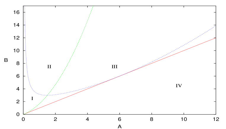
Figure 1: Structure of Roots (for $\Lambda<0$)

curves $B=\frac{1}{3}A(3+2A)$ (green line) and $B=\frac{4}{81}\,\frac{(A+3)^{3}}{A}$ (blue line). For physical interest, we have also plotted the line $A=B$ which represents isotropy. The two curves divides the $(B,A)$ plane in four regions.

Region I

This is the region bounded between the two curves on the left-hand side of their intersection point, with the green line included. One root is negative and two others positive. The positive roots become equal on the blue line and the negative root become zero on the green line. None of the positive roots corresponds to a real infilling solution in the interior of the Berger sphere.

Region II

This is the region above the intersection point of the two curves. So there is one pair of complex roots and a negative root. On the green line there are only a pair of complex roots, the real one being zero.

Region III

Two roots are complex and one is real and positive. The positive root corresponds to a real positive-definite infilling solution in the interior. As above, on the green line, the real root is zero.

Region IV

This is the region bounded by the two lines below their point of intersection, with the blue line included. All roots are positive and one of them corresponds to a real infilling solution. Two roots are equal on the blue line.

5.3 Numerical Study

In the previous section we have studied the general behaviour of the roots systematically. Although $B$ appears only in the constant term of $g(z)$, its role is rather crucial in determining the sign and reality of the roots. In this section we will study the roots of $g(z)$ and their corresponding actions numerically, and demonstrate an interesting connection with catastrophe theory.

First we study the roots and actions for fixed values of $A$, as functions of $B$. From the analysis in the previous section (and from Fig. 1), one would expect to study three distinct generic cases, determined by the value of $A$ less than, equal to and greater than its value where the two curves meet, i.e., at $A=3/2$ (and $B=3$).

Case 1: $A<3/2$

For a fixed $A<3/2$, by varying $B$ one moves continuously from region IV (three positive roots) to the green line where one of the roots become zero (two still being positive), then into region I, where two roots continue to be positive, but the other is now negative, and then to the blue line where the positive roots become equal, and then to region II where they turn complex (the other still being negative).

The behaviour of the three roots and the corresponding Euclidean actions are plotted in Figs. 2 and 3 (as long as they remain real), as functions of $B$ for $A=0.2$ and $A=1$ respectively. (The same colour is used to show the correspondence.)

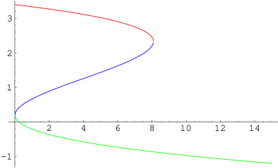
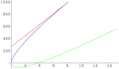
Figure 2: Real Roots and corresponding Actions as functions of $B$ ($A=0.2$)

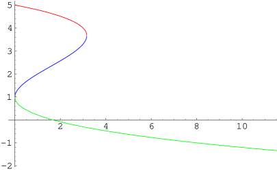
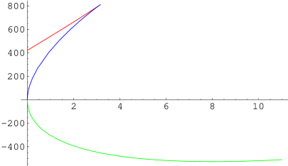
Figure 3: Real Roots and corresponding Actions as functions of $B$ ($A=1$)

Case 2: $A=3/2$

For the special value of $A=3/2$, all roots are positive in region IV, where, on the point that the green and blue lines meet two become equal and the other becomes zero. On entering region II the two equal roots become a complex-conjugate pair and the other turns negative. The behaviour of the three roots is therefore similar to the previous behaviour, except that they all turn complex and become negative at the same value ($B=3$) (Fig. $4$). The corresponding actions also have a structure similar to those in $A<3/2$.

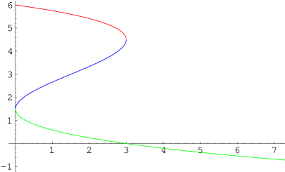
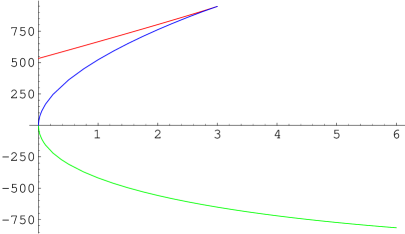
Figure 4: Real Roots and corresponding Actions as functions of $B$ ($A=3/2$)

Case 3: $A>3/2$

For $A>3/2$ one starts in region IV with three positive roots, two of which become equal on the blue line and then turn complex and remain so in region II. The other root remains positive in region III and becomes zero on the green line to become negative in region II. See Fig. $5$ ($A=3$) and Fig. $6$ ($A=100$).

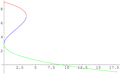
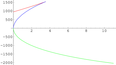
Figure 5: Real Roots and corresponding Actions as functions of $B$ when $A>3/2$ ($A=3$)

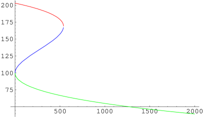
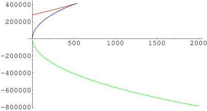
Figure 6: Real Roots and corresponding actions as functions of $B$ for large $A$($A=100$)

The “Catastrophe Manifold” of $I_{E}$

One can see that certain patterns emerge for both $g(z)$ and $I_{E}$. For fixed values of $A$, the real solutions of $g(z)$ form a two-fold pattern as functions of $B$. One can check that this occurs for all $A$, large and small. The upper and lower folds turn over at $B=\frac{4}{81}\frac{(A+3)^{3}}{A}$ and at $B=0$ respectively. This is easily understood with the help of Fig. $1$: the curves (of two roots) in the upper fold meet when the two roots become equal at $B=\frac{4}{81}\frac{(A+3)^{3}}{A}$, i.e., before entering the combined region of II and III where they turn complex. On the other hand, on $B=0$, $g(z)$ has a double root equal to $A$ (the other root is $2A$) – therefore the lower folds turn over around the $B=0$ line. The surface $g(z)=0$ thus formed by placing such images successively (Fig. $11$) is similar in structure to a cusp catastrophe manifold familiar in dynamical systems driven by a quartic potential with two control parameters (see, for example, [20]). The minima of a quartic potential occur when its derivative (a polynomial of degree three) is set to zero and hence the catastrophe manifold represents the equilibrium points of the system. The “catastrophe map” is then the part of projection of the catastrophe manifold onto the plane of the control variables bounded between the lines along which the folds turn over – in our case this is the region bounded between $B=0$ and $B=\frac{4}{81}\frac{(A+3)^{3}}{A}$ curves in Fig. $1$, i.e., the union of region I and IV. However, one may wonder why a cusp does not appear in this case. This is because of the (particular) way in which $A$ and $B$ combine in the coefficients of $g(z)$ and also because they are constrained to be positive – both facts are dictated by the physical configuration. One can obtain a cusp, however, by working with the new variable $D(=AB)$ instead of $B$. A cusp will appear at $A=-3$, which is obviously outside the range of our physical interest.

It is not difficult to see that $I_{E}$ has the same catastrophe map, namely the union of region I and IV. However, the more important observation is that the relative orientation of the folds of $I_{E}$ is the same as that of the corresponding roots of $g(z)$, i.e., they do not cross each other. This pattern persists even when one gets very close to $A=0$ as shown in Fig. $7$. For very small values of $A$ the green and blue lines nearly overlap and coincide completely for $A=0$. They therefore meet the red line at infinity. For higher values of $A$ one gets a persistent behaviour as in Figs. $8$-$10$. Therefore the “catastrophe manifold” of $I_{E}$ is “diffeomorphic” to the one found above for $z$, i.e., the surface $I_{E}$ is obtainable from that of $z$ by a deformation which preserves the catastrophe map. This is not automatic or obvious given the form of $I_{E}$ which is a quadratic function of $z$. Note, however, that the surface of $I_{E}$ is not smooth where the upper fold occurs.

The two-dimensional catastrophe map in a dynamical system with a quartic potential demarcates the regions of three stable minima and one stable minimum. In our case they indicate a demarcation between the regions where there are three real $I_{E}$ and one real $I_{E}$ for the boundary-value problem.

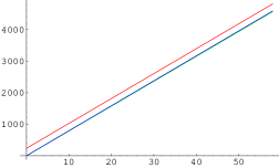
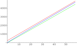
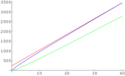
Figure 7: Actions as functions of $B$ ($A=25\times 10^{-6},\,25\times 10^{-4},3\times 10^{-2}$)

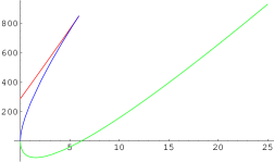
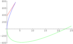
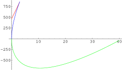
Figure 8: Actions as functions of $B$ ($A=3\times 10^{-1},\,8\times 10^{-1},\,1.2$)

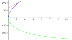
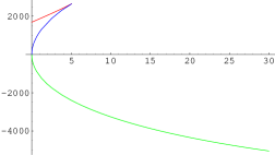
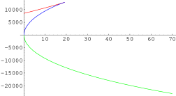
Figure 9: Actions as functions of $B$ ($A=2.0,\,5.0,\,15.0$)

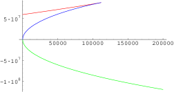
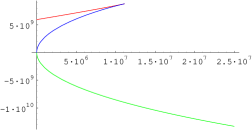
Figure 10: Actions as functions of $B$ ($A=1500,\,15000,\,150000$)

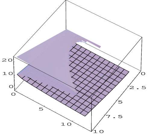
Figure 11: The “catastrophe manifold” $g(z)=0$ : the surface of $I_{E}$ is similar in shape and orientation except at the upper fold where it is not smooth.

5.4 Large Radii and Small Anisotropy

The observations that the space of $I_{E}$ is diffeomorphic to that of $z$ and that it does not intersect itself have immediate physical implications. This means that the dominant contribution will always come from one solution, namely the one represented by the green curve in Figs. $2$-$10$ (and the meshed surface in Fig. $11$). Note that this is the solution which gives a positive-definite infilling solution as long as $b^{2}<\frac{1}{3}a^{2}\,(2a^{2}+3)$. One can verify from Figs. $2$-$6$ that this solution always takes values within the interval $(0,A)$.

In cosmology, one is more interested in regions where $b$ is not greatly different from $a$ and usually when they are both large. All three roots are positive in this latter region. Taking $A=B$, the roots of $g(z)$ are

$$\begin{array}[]{rcl}z_{1}&=&A+\frac{3}{2}-\frac{1}{2}\,\sqrt{12\,A+9},\\ z_{2}&=&2\,A,\\ z_{3}&=&A+\frac{3}{2}+\frac{1}{2}\,\sqrt{12\,A+9}.\\ \end{array}$$ (5.6)

It is easy to check that only $z_{1}<A$ and, hence, $z_{1}$ corresponds to the positive-definite real infilling solution in the interior. The dominant contribution to the path integral (1.1) will therefore come from $z_{1}$ (which can also be checked explicitly in this case). The action of this solution is given by

$$8\pi\,G\,(\lambda I_{E})=-\frac{4}{3}\,{\pi}^{2}\left(-9+3\,\sqrt{12\,A+9}+4\,A\sqrt{12\,A+9}\right)\,\,\sim\,\,-\frac{32}{{\sqrt{3}}}\,{\pi}^{2}\,A^{\frac{3}{2}},$$ (5.7)

so becoming more negative as $A$ grows. Actions for $z_{2}$ and $z_{3}$ are positive and become more positive as $A$ grows, as can be checked explicitly by direct substitution.

6 Conclusion

We have shown that, for a given boundary which is a Berger sphere (a squashed $S^{3}$ with two axes equal), there are in general three distinct ways in which one can fill in with a self-dual Taub-NUT-(anti)de Sitter metric. With suitable choice of variables, the problem of finding explicit solutions for such infilling metrics can be translated into a univariate algebraic equation of degree three and hence can be solved exactly. The Euclidean action $I_{E}$ is a quadratic function of the solutions of this third-degree equation and hence, corresponding to every solution of this equation, the action can be found purely in terms of the boundary data – the two radii $(a,b)$ of the Berger sphere, for both positive and negative cosmological constants. The positive and negative roots of this equation correspond to metrics for which actions are real – only complex solutions correspond to complex-valued actions in general.

In the case of a negative cosmological constant, we have further discussed systematically the ranges of $a$ and $b$ where the solutions of the algebraic system lead to real- and complex-valued solutions in the interior and have studied the structure of the three roots. We found that one of the roots corresponds to a positive-definite infilling solution if and only if $b^{2}<\frac{1}{3}a^{2}\,(2a^{2}+3)$. For small squashing, i.e., when $a$ and $b$ are of the same order and not too small, all three roots are positive. When $a$ and $b$ are exactly equal, this holds for small radius as well. We therefore investigated the roots and their corresponding actions numerically in this range (i.e., until two of them turn complex) as functions of the boundary variables $a$, $b$. We found that both the roots and the actions have structures similar to those of the cusp catastrophe in dynamical systems. The “catastrophe manifold” of $I_{E}$ does not intersect itself which implies that the the dominant contribution will come from the positive-definite infilling solution. Further, the classical actions for large values of the radii $(a,b)$ in their isotropic limit (of particular interest for cosmology) have been discussed. The (dominant) contribution coming from the positive-definite solution has an action proportional to $-a^{3}$, thereby favouring large radii.

Acknowledgements

We would like to thank Gary Gibbons, Stefano Kovacs, Alexei Kovalev, Jorma Louko, Henrik Pedersen, Nick Shepherd-Barron and Galliano Valent for helpful discussions and comments. MMA was supported by awards from the Cambridge Commonwealth Trust and the Overseas Research Scheme.

References

- [1] M. Abramowitz and I. A. Stegun (1965). Handbook of Mathematical Functions (Dover, New York).
- [2] M. F. Atiyah, N. J. Hitchin and I. M. Singer, “Self-duality in four-dimensional Riemannian geometry,” Proc. Roy. Soc. Lond. A 362 (1978) 425.
- [3] S. Barnard, and J. M. Child (1936). Higher Algebra (Macmillan, India).
- [4] B. Carter, “Hamilton-Jacobi And Schrödinger Separable Solutions Of Einstein’s Equations,” Commun. Math. Phys. 10 (1968) 280.
- [5] M. Cvetič, G. W. Gibbons, H. Lu and C. N. Pope, “Bianchi IX Self-dual Einstein Metrics and Singular G(2) Manifolds,” arXiv:hep-th/0206151.
- [6] P. D. D’Eath (1996). Supersymmetric Quantum Cosmology (Cambridge University Press)
- [7] T. Eguchi, P. B. Gilkey and A. J. Hanson, “Gravitation, gauge theories and differential geometry,” Phys. Rep. 66 (1980) 213.
- [8] T. Eguchi and A. J. Hanson, “Asymptotically Flat Self-dual Solutions to Euclidean Gravity,” Phys. Lett. B 74 (1978) 249.
- [9] R. P. Feynman and A. R. Hibbs (1965). Quantum Mechanics and Path Integrals (McGraw-Hill, New York, 1965).
- [10] G. W. Gibbons and S. W. Hawking, “Action Integrals And Partition Functions In Quantum Gravity,” Phys. Rev. D 15 (1977) 2752.
- [11] G. W. Gibbons and S. W. Hawking, “Classification of Gravitational Instanton Symmetries,” Commun. Math. Phys. 66 (1979) 291.
- [12] G. W. Gibbons and C. N. Pope, “ as a Gravitational Instanton,” Commun. Math. Phys. 61 (1978) 239.
- [13] G. W. Gibbons and C. N. Pope, “The Positive Action Conjecture and Asymptotically Euclidean Metrics in Quantum Gravity,” Commun. Math. Phys. 66 (1979) 267.
- [14] J. B. Hartle and S. W. Hawking, “Wave Function of the Universe,” Phys. Rev. D 28 (1983) 2960.
- [15] S. W. Hawking, “Gravitational Instantons,” Phys. Lett. A 60 (1977) 81.
- [16] N. J. Hitchin, “Twistor Spaces, Einstein Metrics and Isomonodromic Deformations,” J. Differential Geom. 42 (1995), no. 1, 30–112.
- [17] L. G. Jensen, J. Louko and P. J. Ruback, “Biaxial Bianchi Type IX Quantum Cosmology,” Nucl. Phys. B 351 (1991) 662.
- [18] D. N. Page, “Taub-Nut Instanton with an Horizon,” Phys. Lett. B 78 (1978) 249.
- [19] H. Pedersen, “Einstein metrics, spinning top motions and monopoles,” Math. Ann. 274 (1986) 35.
- [20] T. Poston and I. Stewart (1978). Catastrophe Theory and its Applications (Pitman, London).
- [21] M. Reid (1988). Undergraduate Algebraic Geometry (Cambridge University Press).
- [22] T. Sakai, “Cut loci of Berger’s spheres”, Hokkaido Math. J. 10(1981), no. 1, 143-155.
- [23] K. P. Tod, “Self-dual Einstein metrics from the Painlevé VI equation,” Phys. Lett. A 190 (1994) 221.
- [24] J. Wess and J. Bagger (1992). Supersymmetry and Supergravity (Princeton University Press).