Abstract

One can try to define the theory of quantum gravity as the sum over geometries. In two dimensions the sum over Euclidean geometries can be performed constructively by the method of dynamical triangulations. One can define a proper-time propagator. This propagator can be used to calculate generalized Hartle-Hawking amplitudes and it can be used to understand the the fractal structure of quantum geometry. In higher dimensions the philosophy of defining the quantum theory, starting from a sum over Euclidean geometries, regularized by a reparametrization invariant cut off which is taken to zero, seems not to lead to an interesting continuum theory. The reason for this is the dominance of singular Euclidean geometries. Lorentzian geometries with a global causal structure are less singular. Using the framework of dynamical triangulations it is possible to give a constructive definition of the sum over such geometries, In two dimensions the theory can be solved analytically. It differs from two-dimensional Euclidean quantum gravity, and the relation between the two theories can be understood. In three dimensions the theory avoids the pathologies of three-dimensional Euclidean quantum gravity. General properties of the four-dimensional discretized theory have been established, but a detailed study of the continuum limit in the spirit of the renormalization group and asymptotic safety is till awaiting.

1 Introduction

We are still searching for the theory of quantum gravity. While the four dimensional theory of quantum gravity may have to go beyond the conventional framework of quantum field theory it is possible to discuss two- and three-dimensional quantum gravity in terms of conventional field theoretical concepts. In this way one may hope to learn important lessons about the “real” theory of four-dimensional gravity, whether or not it can be defined as a non-perturbative quantum field theory.

Two-dimensional quantum gravity is an example of the subtlety present in a reparameterization invariant theory. In two dimensions the Einstein action is trivial as long as we do not sum over different topologies of space-time (which we are not attempting here). Thus we are left only with the cosmological term in the action and the classical theory is trivial. Diffeomorphism invariance ensures that no field degrees of freedom exist. Nevertheless, a finite number of quantum mechanical degrees of freedom survives, which still have a rich (quantum) geometrical description. Despite the fact that no field degrees of freedom exist, it still makes sense to talk about generalized Hartle-Hawking like amplitudes: the sum over all Euclidean two-geometries with boundaries of of lengths $L_{k}$, $k\!=\!1,\ldots,n$. Similarly one can define the concept of correlators, depending on geodesic distance and show that standard concepts, derived from Euclidean quantum field theory or the theory of critical phenomena, make sense even in a framework of fluctuating geometries.

Three-dimensional quantum gravity can be addressed in the same spirit. The new aspects of three-dimensional quantum gravity compared to two-dimensional quantum gravity are the following: the theory is a perturbative non-renormalizable theory in the gravitational coupling constant and the Euclidean action is unbounded from below. It is thus a priori unclear how to make sense of an Euclidean three-dimensional path integral. On the other hand we know that the conformal factor only appears as a constraint in a reduced phase-space quantization and thus should not really pose a problem in a Lorentzian quantization of three-dimensional quantum gravity. It is of interest to understand if it is possible at all to think about three-dimensional quantum gravity as a path integral involving the sum over a certain class of three-dimensional Euclidean geometries of a given topology.

Contrary to the situation in two dimensions this “purely” Euclidean approach has not been successful in three dimensions. This led to the concept of “Lorentzian” gravity, the idea being that only Lorentzian geometries with a global causal structure should be included in the path integral, and that a possible rotation to Euclidean geometries should respect this. Returning to two-dimensional quantum gravity where analytic solutions can be found, one can implement this program and one finds that Lorentzian quantum gravity is different from Euclidean quantum gravity. Using proper-time as an evolution parameter, two-dimension Euclidean quantum gravity can be understood as two-dimensional Lorentzian quantum gravity where it is possible to create at each space-time point a baby universe, which at later proper-time remains separated from the “parent” universe. In three-dimensions the path-integral over Lorentzian geometries can be studied by numerical as well as analytical methods, and it seems an interesting candidate for a theory of quantum gravity, defined as the sum over geometries, with relative weights dictated by the Einstein-Hilbert action.

2 Non-perturbative regularization

In a theory of quantum gravity it is not enough to study perturbation theory. The examples of the $\phi^{4}$ field theory and $QCD$ in four dimensions illustrates this. Both theories have well defined perturbative expansions, and observables can be calculated to any order in the coupling constant in both theories. Since both theories are renormalizable one can express the observables entirely in terms of the renormalized mass and coupling constant. However, it does not ensure that a genuine quantum field exists without a cut-off. In order to address this question one first has to define the theory outside perturbation theory and then show that observables calculated in the non-perturbatively defined theory become independent of a possible cut-off, used in the definition of the non-perturbative framework. Finally, one can then discuss to what extend the perturbation expansion, which is usually at most an asymptotic expansion, contains information about the non-perturbatively defined theory.

All the evidence suggests that $QCD$ exists as a genuine quantum field theory in four-dimensional space-time. One needs a cut-off at an intermediate step when defining the theory, but this cut off will never show up in any continuum physical observables. The situation is opposite for the $\phi^{4}$ theory. It seems impossible to define a non-trivial theory where the renormalized coupling constant is different from zero when the cut-off is removed. This situation is of course already hinted by low order perturbation theory where one observes a Landau pole at large energies.

In the case of a $\phi^{4}$ theory, as it appears for instance in the Standard Model, one considers it as an effective low energy approximation to a more more elaborate, yet to be understood, theory at the GUT scale or the Planck scale. Clearly, if we want to apply conventional quantum field theoretical concepts to the theory of quantum gravity, such a situation is not good enough: it has to be a quantum theory independent of cut-off in the same way as $QCD$, since the quantum phenomena we want to consider take place precisely at the Planck scale. In order to understand whether or not the theory exists as a conventional quantum theory a non-perturbative framework is thus mandatory.

For non-Abelian gauge theories and the $\phi^{4}$ scalar field theory the use of a space-time lattice has provided a useful regularization, in particularly when combined with the use of Monte Carlo simulations, taking advantage of the fast present days computers. It has allowed us to related Euclidean quantum field theory to the statistical theory of critical phenomena. Stated very shortly Euclidean quantum field theories can be extracted from second order phase transitions of generalized spin systems defined on the lattice. The way the continuum field theory is recovered from the lattice spin model is as follows: by fine-tuning the coupling constants of the model , generically denoted $\lambda$, one can approach the phase transition point $\lambda_{c}$. The spin-spin correlation length $\xi$, measured in lattice spacings, will diverge as

$$\xi(\lambda)\sim\frac{1}{|\lambda-\lambda_{c}|^{\nu}}.$$ (1)

The lattice spacing $a$ serves as the cut-off. By Fourier transformation it is seen that the (lattice) momentum must be less that $\pi/a$. We introduce the physical correlation length $L$ as $L\!=\!\xi(\lambda)\cdot a$. One now take the limit

$$L=\xi(\lambda)\cdot a~{}~{}~{}{\rm fixed},~{}~{}~{}\xi(\lambda)\to\infty,~{}~{}~{}~{}a\to 0.$$ (2)

From eq. (1) we see that the interpretation of this continuum limit is that while the correlation length measured in lattice units diverges when $\lambda\to\lambda_{c}$, the lattice spacing (the cut-off) goes to zero as:

$$a(\lambda)\sim|\lambda-\lambda_{c}|^{\nu}~{}~{}~{}{\rm for}~{}~{}~{}\lambda\to\lambda_{c}.$$ (3)

In this scaling limit the lattice becomes increasingly fine-grained compared to the physical correlation length $L$. The lattice structure becomes unimportant for the physics associated with these long range fluctuations and Euclidean invariance will be restored for the physics related to these fluctuations. Let $\phi(x_{n})$ denote the spin at lattice point $x_{n}\!=\!n\cdot a$. Since the spin correlation functions will behaves

$$\langle\phi(x_{n})\phi(0)\rangle\sim\mbox{e}^{-n/\xi(\lambda)}\sim\mbox{e}^{-x_{n}/L}$$ (4)

for large $n$, we see that the renormalized physical mass should be identified with $1/L$:

$$m_{ph}=1/L.$$ (5)

The choice of physical correlation length in (2) is equivalent to a choice of renormalized mass in the continuum quantum field theory. We have used $\lambda$ as a generic coupling constant and usually the “spin” system will have a number of coupling constants. Combined fine-tuning will allow to fix in addition the other renormalized coupling constants of the continuum theory. Finally the lattice “spin” $\phi(x_{n})$ is assigned a dimension from the short distance behavior of the spin-spin correlation function. In eq. (4) it was assumed that $n\gg\xi(\lambda)$. In the opposite limit $1\ll n\ll\xi(\lambda)$ one expects

$$\langle\phi(x_{n})\phi(0)\rangle\sim n^{-d+2+\eta}\sim\frac{a^{d-2+\eta}}{x_{n}^{d-2+\eta}},~{}~{}~{}~{}a\ll x_{n}\ll L.$$ (6)

The factor $a^{d-2+\eta}$ reflects the scaling dimension of the physical field

$$\phi_{phys}=a^{-(d-2+\eta)/2}\phi_{lattice},$$ (7)

and the anomalous scaling dimension $\eta$ is related to wave function renormalization.

This way of defining a quantum field theory is closely related to use of the renormalization group in quantum field theory and it emphasizes the concept of universality: many different “spin” systems defined on lattices will lead to the same class of continuum field theories, characterized by critical exponents like $\nu$ and $\eta$. One can imagine an idealized spin system where all possible spin interactions are included in the spin Hamiltonian. The key assumption is then that in this infinite dimensional coupling constant space the critical surfaces where one can define continuum theories are of finite co-dimensions. Thus there is only a finite number of coupling constants which need to be fine-tuned in order that the system becomes critical. Translated to continuum physics only a finite number of coupling constants need renormalizations. In the context of a perturbative expansion around free field theory this leads to the usual concept of renormalizable theories. But the philosophy also applies to expansions about non-trivial critical points where there exist no free fields. Since four-dimensional quantum gravity is not renormalizable viewed as a perturbation theory around flat space, the simplest possible scenario still using the framework of conventional quantum field theory is that of a non-trivial fixed point in the sense described above. In the context of quantum gravity this was first emphasized by Weinberg, who called it “asymptotic safety” since only a finite number of coupling constants needed adjustment in order to recover continuum physics.

While the lattice formulation of quantum field theories has the virtues mentioned above it also has a number of drawbacks:

• The lattice formulation is usually not a convenient framework for analytic calculations.

• space-time symmetries are explicitly broken. In particular, the lattice seems not to be the best regularization for theories with local space-time symmetries.

It is no necessarily so. Two-dimensional Euclidean quantum gravity provides a counter example. There exists a simple lattice regularization of 2d Euclidean quantum gravity, called dynamical triangulation, which is

• convenient for analytic calculations,

• has no problems recovering the diffeomorphism invariant continuum limit,

• is defined directly on the space of geometries,

• serves as a textbook example of universality when viewed as a statistical field theory.

The use of dynamical triangulations is an attempt to approximate the space of geometries by the class of piecewise linear geometries which can be constructed from an elementary building block. In two dimensions the building block is an equilateral triangle and the piecewise linear geometries are obtained by gluing together the triangles in all possible ways consistent with a given two-dimensional topology. If we consider the triangles as flat, the (piecewise linear) geometry is uniquely determined by the connectivity pattern of the triangulation. The length $a$ of the links serves as the cut-off as for a regular lattice, and with the interpretation given here it is a diffeomorphism invariant cut-off, since we work directly with geometries. The hope is that when $a\to 0$ this set of geometries will be “dense” in the set of all geometries which enters into the path integral. Also, it is important to understand that in the spirit of universality there is nothing special about the use of equilateral triangles. For instance, one could have used squares as building blocks, and if we wanted a piecewise linear geometry associated with such generalized “quadrangulations” one could subdivide the square into two triangles at one of the diagonals, considering each triangle as “flat”. The results we will mention in the following will indeed be independent of such details.

Using a lattice to define the path integral also includes defining the discretized action. In conventional lattice theories the action is usually chosen such that it for $a\to 0$ converges to the classical continuum action of the field theory one tries to quantize. There is a large freedom in choosing such discretized actions, all leading to the same continuum theory by the universality mentioned above. In the case of piecewise linear geometries the Einstein-Hilbert action can actually be implemented entirely in terms of the piecewise linear geometry, as first noted by Regge [5]. For a piecewise linear d-dimensional geometry the integrated curvature is

$$\int\mbox{d}^{d}\xi\sqrt{g}\,R=\sum_{\sigma_{d-2}}V(\sigma_{d-2})\,\varepsilon(\sigma_{d-2}),$$ (8)

where $\sigma_{d-2}$ denotes a $(d\!-\!2)$-dimensional simplex in the $d$-dimensional triangulation, $V(\sigma_{d-2})$ the volume of the simplex and $\varepsilon(\sigma_{d-2})$ the deficit angle associated with the simplex. Eq. (8) is “exact” in the sense that it is the natural curvature one can associate to a piecewise linear geometry. As an example it leads to Eulers formula in the case of two-dimensional manifolds.

In our case it becomes even simpler because the piecewise linear geometries are constructed from a fundamental building block. The space-time volume is thus proportional to the total number of building blocks and the curvature associated with a $(d\!-\!2)$-simplex $\sigma_{d\!-\!2}$ is related to the number $o(\sigma_{d\!-\!2})$ of $d$-simplices sharing it in the following way: call the angle in a $d$-simplex between two $(d\!-\!1)$-simplices sharing a $(d-2)$-simplex $\theta$. Then the deficit angle associated with $\sigma_{d\!-\!2}$ is

$$\varepsilon(\sigma_{d\!-\!2})=2\pi-\theta\,o(\sigma_{d\!-\!1}).$$ (9)

The Einstein-Hilbert action

$$S[g]=-\frac{1}{G}\int\mbox{d}^{d}\xi\sqrt{g}R+\Lambda\int\mbox{d}^{d}\xi\sqrt{g}$$ (10)

associated with this kind of piecewise linear geometries is thus very simple and can be expressed as

$$S_{T}=-k_{d-2}N_{d-2}(T)+k_{d}N_{d},$$ (11)

where $N_{d-2}(T)$ denotes the number of $(d\!-\!2)$-simplices and $N_{d}(T)$ denotes the number of $d$-simplices of the triangulation $T$. The dimensionless coupling constants $k_{d\!-\!2}$ and $k_{d}$ are related to the coupling constants $G$ and $\Lambda$ as

$$k_{d-2}\sim\frac{a^{d-2}}{G},~{}~{}~{}~{}~{}k_{d}\sim\frac{a^{d-2}}{G}+a^{d}\Lambda.$$ (12)

This has the implication that in any dimension the calculation of the functional integral associated with the Einstein-Hilbert action is purely combinatorial:

$$Z(G,\Lambda)=\int{\cal D}[g_{\mu\nu}]\;\mbox{e}^{-S[g]}~{}~{}\to~{}~{}Z(k_{d\!-\!2},k_{d})=\sum_{T}\mbox{e}^{-S_{T}},$$ (13)

where the sum can be rewritten as

$$Z(x,y)=\sum_{N_{d},N_{d\!-\!2}}x^{N_{d}}y^{N_{d\!-\!2}}{\cal N}(N_{d},N_{d\!-\!2}).$$ (14)

In this formula $x\!=\!e^{k_{d\!-\!2}}$, $y\!=\!e^{-k_{d}}$ and ${\cal N}(N_{d},N_{d\!-\!2})$ denotes the number of different piecewise linear geometries one can construct from $N_{d}$ simplices, having $N_{d\!-\!2}$ $(d\!-\!2)$-simplices. In this way the partition function $Z(x,y)$ becomes the generating function for the numbers ${\cal N}(N_{d},N_{d\!-\!2})$ as it is used in standard combinatorial analysis. This kind of remarkable simplification is only possible because we have restricted the sum over geometries to the ones with can be constructed from the cut-off size building blocks and because the Einstein action by the Regge-prescription is very simple for piecewise linear geometries.

2.1 The continuum limit

The combinatorial aspect of the sum over geometries allows us to understand how to approach the continuum limit in the simplest situations: the number of geometries of a given space-time topology and space-time volume grows exponentially with space-time volume:

$$\sum_{N_{d\!-\!2}}{\cal N}(N_{d\!-\!2},N_{d})\sim\mbox{e}^{k_{d}^{c}N_{d}+o(N_{d})}.$$ (15)

From this it follows that for each value of $k_{d\!-\!2}$ there exists a critical value $k_{d}^{c}(k_{d\!-\!2})$ such that

• For $k_{d}>k_{d}^{c}(k_{d\!-\!2})$ the partition function $Z(k_{d\!-\!2},k_{d})$ is convergent, while it is divergent for $k_{d}<k_{d}^{c}(k_{d\!-\!2})$.

• The infinite volume limit is obtained by fine-tuning $k_{d}\to k_{d}^{c}(k_{d\!-\!2})$. This can be viewed as an additive renormalization of the bare “cosmological” constant:

  $$k_{d}=k_{d}^{c}(k_{d\!-\!2})+\Lambda a^{d},$$ (16)

  where $\Lambda$ is viewed as a renormalized cosmological constant.

• It might require an additional fine-tuning of $k_{d\!-\!2}$ to obtain a continuum limit, if it exists at all. Such a fine-tuning can be viewed as a renormalization of the gravitational coupling constant. (The analogy with the spin models might be helpful: the infinite volume limit means that the lattice is infinite, but it does not imply that we have a continuum field theory. That might require a fine-tuning of the coupling constants of the spin model).

If a continuum limit of the kind discussed above can be constructed, the corresponding quantum field theory might serve as a candidate for the asymptotic safe non-renormalizable theory in the sense of Weinberg.

3 Two-dimensional Euclidean quantum gravity

3.1 Hartle-Hawking wave functions

Two-dimensional gravity, defined via dynamical triangulations, serves as a test of some of the above mentioned ideas. The integral of the curvature term is a topological invariant in two dimensions. Thus, as long as we do not consider topology changes of space-time we can ignore the curvature term in two dimensions and we are left with the cosmological term. We write:

$$Z_{a}(k_{2})=\sum_{T}\mbox{e}^{-k_{2}N_{2}(T)}=\sum_{N}\mbox{e}^{-k_{2}N}{\cal N}(N),$$ (17)

where ${\cal N}(N)$ denotes the number of different triangulations constructed from $N$ equilateral triangles with link length $a$. Objects of interest in the context of quantum gravity are the (generalized) Hartle-Hawking wave functions where the geometry of spatial boundaries are kept fixed, and the amplitude for such a configuration is obtained by summing over all two-dimensional geometries which have the prescribed spatial boundary geometries. In two dimensions the geometry of the boundary is uniquely fixed by its length. In the regularization mentioned above a boundary will consist of $l$ links of length $a$ from the adjacent triangles. The length of the boundary is thus $L\!=\!l\cdot a$. The regularized Hartle-Hawking wave function can thus be written as

$$G_{a}(l_{1},\ldots,l_{n};k_{2})=\sum_{T(l_{1},\ldots,l_{n})}\mbox{e}^{-k_{2}N_{2}(T)}=\sum_{N}\mbox{e}^{-k_{2}N}{\cal N}_{l_{1},\ldots,l_{n}}(N),$$ (18)

where ${\cal N}_{l_{1},\ldots,l_{n}}(N)$ denotes the number of different triangulations constructed from $N$ triangles and with $n$ boundaries consisting of $l_{1},\ldots,l_{n}$ links, respectively.

It is seen that the calculation of $Z_{a}(k_{2})$ and $G_{a}(l_{1},\ldots,l_{n};k_{2})$ can be reduced to purely combinatorial problems: the counting of distinct triangulations of various kinds. One finds, using either combinatorial methods or so-called matrix models, that

$${\cal N}(N)\sim\mbox{e}^{k_{2}^{c}N}N^{\gamma-3},$$ (19)

where $\sim$ means the leading asymptotic behavior when $N$ is large, and where $\gamma$ depends on the topology of two-dimensional space-time. For the simplest topology of a sphere $\gamma\!=\!-1/2$. Thus we find

$$Z_{a}(k_{2})\sim\sum_{N}\mbox{e}^{-(k_{2}-k_{2}^{c})N}\;N^{\gamma-3}\sim\frac{1}{(k_{2}-k_{2}^{c})^{\gamma-2}}.$$ (20)

One observes a singular structure for $k_{2}\to k_{2}^{c}$ which governs the large $N$ behavior of the sum, and a continuum limit can be obtained by an additive renormalization of the cosmological constant:

$$k_{2}=k_{2}^{c}+a^{2}\Lambda.$$ (21)

An additive renormalization is expected since $\Lambda$ has a positive mass dimension. The renormalization is “natural” in the sense that

$$(k_{2}-k_{2}^{c})N=(\Lambda a^{2})N=\Lambda(a^{2}N)=\Lambda\,V,$$ (22)

where $V$ denotes the continuum space-time volume. The partition function becomes

$$Z_{a}(k_{2})\sim(a^{2}\Lambda)^{2-\gamma}\sim a^{2-\gamma}\cdot Z(\Lambda),~{}~{}~{}~{}Z(\Lambda)=\Lambda^{2-\gamma}.$$ (23)

The divergent $a$-factor can be viewed as the kind of wave function renormalization which is always present in the path integral version of quantum field theory.

The counting can also be performed in the case of triangulations with boundaries. The result is as follows:

$${\cal N}_{l_{1},\ldots,l_{n}}(N)\sim\mbox{e}^{k_{2}N}\mbox{e}^{k_{b}(l_{1}+\cdots+l_{n})}N^{\gamma_{n}}(l_{1}\cdots l_{n})^{\gamma_{b}}F(l_{i}/\sqrt{N}).$$ (24)

The exponential growth with $N$ is counteracted by a renormalization of the cosmological constant as above while the exponential growth with respect to the boundary length can be controlled by adding a boundary cosmological constant to the action. This should anyway be done when we have space-like boundaries (see [6] for details). In this way we can take a continuum limit by scaling $l_{i}\sim\sqrt{N}$, which is what one expects from the canonical dimensions of boundaries and bulk in two-dimensional quantum gravity. The resulting continuum Hartle-Hawking wave functions can be found (see [6, 7]). We list the results in the case three boundaries (which is particularly simple):

$$G(L_{1},L_{2},L_{3},\Lambda)=\Lambda^{-1/2}\sqrt{L_{1}L_{2}L_{3}}\;\mbox{e}^{-\sqrt{L}(L_{1}+L_{2}+L_{3})}.$$ (25)

3.2 Universality

It is important to understand that the results mentioned above are universal. The precise nature of the short distance regularization used is not important. We could have constructed our two-dimensional complexes from any combination of triangles, squares, pentagons etc with relative weights $g_{3},g_{4},g_{5},\ldots$ and we would have obtained the same continuum Hartle-Hawking wave function as long as the relative weights of the various kinds of polygons are non-negative. If some of the weights are taken negative the system can no longer be given a simple interpretation as two-dimensional quantum gravity. However, it can be shown that they can be given the interpretation as certain matter fields coupled to two-dimensional random lattices of the kind used above in constructing the theory of two-dimensional quantum gravity. The fine-tuning of the coupling constants give us new continuum systems which can be viewed as certain conformal field theories coupled to two-dimensional quantum gravity [6, 8, 9].

Thus we can view these generalized systems as a school book example of critical systems: they are defined in an infinite dimensional coupling constant space $g_{3},g_{4},\ldots$. Fine-tuning the coupling constants bring us to a critical hyper-surface of co-dimension one, describing two-dimensional quantum gravity, and further fine-tuning leads to the critical behavior of certain conformal field theories coupled to two-dimensional quantum gravity. The critical exponents of the conformal field theories are changed (relative to their value in flat two-dimensional space) due to the influence of the fluctuating geometry, and likewise the behavior of two-dimensional quantum gravity is changed by the back-reaction of matter (see [6] for details).

3.3 Quantum geodesic distance

The critical behavior of the conformal field theories coupled to quantum gravity can be calculated by looking at globally defined matter correlators. Let $\phi(x)$ be a scalar matter field. Then

$$\int{\cal D}[g(x)]{\cal D}\phi(x)\;\mbox{e}^{-S[g,\phi]}\int\mbox{d}^{2}x\sqrt{g(x)}\int\mbox{d}^{2}y\sqrt{g(y)}\;\phi(x)\phi(y)$$ (26)

is reparameterization invariant and the scaling behavior of this correlator with respect to the cosmological constant $\Lambda$ determines the scaling dimension of the fields and the critical exponents. The reason for this is that the average volume of space-time is monitored by the cosmological constant,

$$\langle V\rangle\sim\Lambda^{-1},$$ (27)

and thus the finite-size scaling relations of the system are determined as functions of the cosmological constant.

However, from the theory of critical phenomena we know that the underlying universality of large scale fluctuations originating from quite different microscopic interactions is due to a divergent correlation length $\xi(g_{3},g_{4},\ldots)$. How do we define such a length in quantum gravity? An object like $\langle\phi(x)\phi(y)\rangle$ has clearly no reparameterization invariant meaning if we view $x$ and $y$ as coordinates. Further, we have to integrate over all geometries and the (geodesic) distance between $x$ and $y$ will vary. One can define the concept of an invariance correlation function as follows [10, 11]:

$$\langle\phi(D)\phi(0)\rangle \equiv \int{\cal D}[g(z)]{\cal D}\phi(z)\;\mbox{e}^{-S[g,\phi]}$$

$$\int\mbox{d}^{2}x\sqrt{g(x)}\int\mbox{d}^{2}y\sqrt{g(y)}\;\delta\Big{(}D_{g}(x,y)-D\Big{)}\,\phi(x)\phi(y).$$

In (3.3) $D_{g}(x,y)$ denotes the geodesic distance between the space-time points labeled $x$ and $y$. Let us consider the simplest case where there are no matter Lagrangian at all and $\phi(x)\!=\!1$ in (3.3). In this case (3.3) can be viewed as the partition function $G(D)$ for universes where two marked points are separated a given geodesic distance $D$. Again the calculation of this partition function reduces to the combinatorial problem of counting a certain class of two-geometries. And again one can solve the combinatorial problem. In the regularized theory one obtains for $k_{2}$ close to the critical point [10]:

$$G_{a}(d;k_{2})=(k_{2}-k_{2}^{c})^{3/4}\frac{\cosh d\sqrt[4]{k_{2}-k_{2}^{c}}\,d}{\sinh^{3}d\sqrt[4]{k_{2}-k_{2}^{c}}}.$$ (29)

Here $d$ denotes a suitable discretized geodesic distance 

If we take the continuum limit for the above “two-point” function it is seen that we are forced to scale geodesic distance anomalously:

$$D=d\sqrt{a}.$$ (30)

With this scaling we obtain

$$G(D;\Lambda)=\Lambda^{3/4}\frac{\cosh\sqrt[4]{\Lambda}D}{\sinh^{3}\sqrt[4]{\Lambda}D}.$$ (31)

This function behaves as two-point function: it falls of exponentially for large distances and it behaves power-like for distances smaller that $1/\sqrt[4]{\Lambda}$. The anomalous dimension of the geodesic distance is also reflected in the average space-time volume $V$ enclosed in disc of (geodesic) radius $D$. One finds

$$\langle V\rangle_{D}\sim R^{4},~{}~{}~{}~{}~{}~{}R\ll 1/\sqrt[4]{\Lambda}.$$ (32)

Thus the Hausdorff dimension of a typical two-dimensional geometry is four, as first realized in [12]. This is a genuine quantum phenomenon.

Until now it has not been possible to calculate analytically the two-point function (3.3) when matter fields are present. However, it can be studied numerically and it can be verified that for the Ising model and the three-state Potts model coupled to two-dimensional quantum gravity one really obtains a divergent spin-spin correlation length when the spin couplings approach their critical values (see [13, 14] for details).

3.4 The proper-time propagator and quantum geometry

An important tool used in the calculation of $G(D;\Lambda)$ is the proper-time propagator. In Euclidean geometry proper-time $T$ is equivalent to geodesic distance, which we have denoted $D$. Let $B_{1}$ be a boundary. The distance of a point $P$ to $B_{1}$ is defined as the minimal geodesic distance of $P$ to the points of $B_{1}$. We define another boundary $B_{2}$ to be separated from it by a geodesic distance $D$, or proper-time $T$, if the distance of each point on $B_{2}$ to $B_{1}$ is $D$ (note that the definition is asymmetric with respect to $B_{1}$ and $B_{2}$). The proper-time propagator $G_{\Lambda}(B_{1},B_{2};T)$ is defined by summing over all two-geometries with boundaries $B_{1}$ and $B_{2}$, such that $B_{2}$ has geodesic distance $T$ to $B_{1}$, the weight of each configuration given as usually by $\mbox{e}^{-S}$. It was first calculated in [12], and in [15] it was shown that the equation which determines it can be obtained by very simple “quantum geometric” reasoning. Consider Fig. 1. It shows a disc amplitude with one marked interior point $P$ (the marked point on the boundary is irrelevant for the considerations to follow)

Figure 1: A geometry contributing to the punctured disc amplitude (the punctured Hartle-Hawking wave function), decomposed into geometries contributing to the proper-time propagator and the disc amplitude.

Since $P$ can be anywhere, marking a point corresponds to multiplying with the space-time volume $V$ or (equivalently) differentiating after the cosmological constant. However, one can also make the following decomposition: $P$ has a geodesic distance $T$ to the boundary “1”. Form the connected loop through $P$ which has distance $T$ to the boundary. One obtains all geometries with one marked point by integrating over $T$ and the length of the loop through $P$. We thus have the following consistency equation involving the Hartle-Hawking wave function and the proper-time propagator:

$$\frac{\partial G(L_{1};\Lambda)}{\partial\Lambda}=\int\mbox{d}T\mbox{d}L_{2}\;G_{\Lambda}(L_{1},L_{2};T)G(L_{2};\Lambda)$$ (33)

Under reasonable scaling assumptions one can show that eq. (33) determines the behavior of both $G(L;\Lambda)$ and $G_{\Lambda}(L_{1},L_{2};T)$. Quite surprisingly one finds two different solutions [15]. One scaling behavior leads to the Hartle-Hawking wave function already encountered. The other consistent scaling behavior leads to a different two-dimensional theory of quantum gravity which we call “Lorentzian” quantum gravity for reasons which will become clear in Sec. 5. At the moment we concentrate on the “Euclidean” quantum gravity theory discussed until now. Rather than discussing the explicit form of the proper-time propagator, let us give a further example of simple relations derived using “quantum geometry” (for more examples and a description of “operator product expansions” in two-dimensional quantum gravity see [16]). The example will illustrate that the proper-time propagator contains all information about quantum gravity. We have already mentioned that the usual Hartle-Hawking wave function $G(L;\Lambda)$ can be derived from properties of $G_{\Lambda}(L_{1},L_{2};T)$. Let us consider instead the two-loop function $G(L_{1},L_{2};\Lambda)$. It is not simply obtained from by integrating $G_{\Lambda}(L_{1},L_{2};T)$ over $T$ since boundary “2” of the space-times included in $G_{\Lambda}(L_{1},L_{2};T)$ has a well-defined distance to boundary “1”. No such relation exists between the boundaries in $G(L_{1},L_{2};\Lambda)$. However, starting at boundary “1” and moving in successive proper-time steps one will end in the situation shown in Fig. 2.

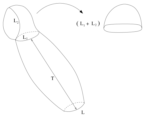
Figure 2: A geometry contributing to $G(L,L_{2};\Lambda)$ decomposed into geometries contributing to $G_{\Lambda}(L,L_{1};T)$ and $G_{fig\!-\!8}(L_{1}+L_{2};\Lambda)$. The latter is related to the disc amplitude (the Hartle-Hawking wave function) $G(L_{1}+L_{2};\Lambda)$ as shown.

The “figure 8” amplitude [17] with a boundary of length $L$ is related to the disc amplitude by

$$G_{fig-8}(L;\Lambda)\sim LG(L;\Lambda),$$ (34)

simply because it is obtained by pinching the boundary of the disc amplitude. Finally we can write:

$$G(L_{1},L_{2};\Lambda)=\int\mbox{d}T\mbox{d}L_{3}\;G_{\Lambda}(L_{1},L_{3};T)\,(L_{2}+L_{3})G(L_{2}+L_{3};\Lambda).$$ (35)

Like the expression for the disc amplitude, which could be derived from general properties of the proper-time propagator, (35) is also an example of “quantum geometric” considerations, which in essence are just combinatorial identities.

3.5 Summary

Euclidean two-dimensional quantum gravity as described above as the continuum limit of a regularized theory of two-dimensional geometries is still awaiting a precise mathematical description. What is meant by this is the following: Consider the random walk process in $R^{d}$. One can take the continuum limit in much the same way as we did in the construction of $G(L_{1},\ldots,L_{n};\Lambda)$. The number of random walks between point $x$ and $y$ in $R^{d}$ grows exponentially with the number of steps in the random walk process and by fine-tuning the fugacity or stopping probability of the random walk process one can obtain the relativistic scalar particle propagator from point $x$ to point $y$. This is in fact the typical “first quantized” path integral derivation of the free propagator. In this case we know the correct mathematical measure on the space of continuous path from $x$ to $y$: it is the Wiener measure . We would like to construct the corresponding measure on the space of two-dimensional continuous geometries. It should exist! Let us list the analogies between the the random walk and the “random geometries”: Their numbers grow exponentially with the number of “elements” (steps in the random walk, triangles etc in the case of random geometries). The constants in the exponents are non-universal, but the leading corrections to the exponential growth are universal. A “typical” path or random geometry is fractal, in fact in almost the same way. The length of a “typical” path between $x$ and $y$ grows like $|x\!-\!y|^{2}$ rather than like $|x\!-\!y|$. In the same way the area of a random two-geometry of (geodesic) diameter $D$ grows as $D^{4}$ rather than $D^{2}$. It thus seems that the class of continuous two-dimensional geometries constitutes a well-defined class of geometries, not much “wilder” than the class of continuous path . Our results suggest that it should be possible to define a measure on this set, since we can constructively define the path integral over the set of two-geometries.

Some of the results mentioned above can be “guessed” from the continuum formulation of two-dimensional quantum gravity known as “Liouville quantum gravity”. Let us consider a fixed topology, for instance that of the sphere, which we represent as the complex plane with $\infty$ identified as the north-pole. Any metric can be decomposed as

$$g_{\mu\nu}=\mbox{e}^{\phi}\delta_{\mu\nu},$$ (36)

and has to satisfy certain regularity conditions at $\infty$. The corresponding classical action is simply

$$S=\Lambda\int\mbox{d}^{2}x\sqrt{g}=\Lambda\int\mbox{d}^{2}x\;\mbox{e}^{\phi}.$$ (37)

However, $\phi(x)$ is not a genuine dynamical field and the kinetic term comes entirely from the gauge fixing in the path integral:

$$Z(\Lambda)=\int{\cal D}\phi\;\mbox{e}^{-\int\mbox{d}^{2}x(\Lambda\mbox{e}^{\phi}+\alpha(\partial\phi)^{2})}.$$ (38)

There are two problems associated with this partition function. The first is that a cut-off $a$ should be invariant under reparameterization, i.e.

$$a^{2}=\mbox{e}^{\phi(x)}(dx_{1}^{2}+dx_{2}^{2}),$$ (39)

and the cut-off in parameter space $R^{2}$ is thus field dependent. The next problem is the geometric observables we have discussed so far become non-local and complicated when formulated in terms of $\phi(x)$. For instant the concept of geodesic distance as used above in the combinatorial approach is difficult to treat in terms of $\phi(x)$. Nevertheless, a number of the results from the combinatorial approach has been verified in quantum Liouville theory via the study of vertex operators of the theory in the following sense: the study of the scaling properties of vertex operators allows one to make reasonable guesses of the scaling behavior of the “observables” $G(L_{1},\ldots,L_{n};\Lambda)$ and in this way recover the results obtained constructively by combinatorial methods (see for instance [18]). It is worth emphasizing this, because it shows that there is an underlying continuum quantum theory at the critical point of the discretized theory, described by a Lagrangian and some standard rules of quantization, which however are technically difficult to implement because of the reparameterization invariance of the theory.

4 Higher dimensions

Encouraged by the success of two-dimensional Euclidean quantum gravity one can try to follow the program outlined in the introduction and look for a non-trivial fixed point of four-dimensional quantum gravity in the spirit of asymptotic safety as defined by Weinberg. It is indeed possible to find a candidate fixed point using the simplest action mentioned in Sec. 2 [19, 20]. This fixed point seemed originally to relate in very interesting ways to various other proposals for a theory quantum gravity [21, 22], but extensive computer simulations eventually established that the phase transition was a (weakly) first order transition [23] and thus could not serve as the desired fixed point of second or higher order . In terms of the properties of “typical” configurations of four-dimensional Euclidean geometries there is a sharp contrast with the two-dimensional case: a typical geometry, constructed by gluing together equilateral four-simplices with weight “one” is singular: the four-dimensional space-time volume grows at least exponentially with geodesic radius of the universe: Thus one cannot talk about a definite fractal dimension of a “typical” geometry. The first order phase transition observed in the numerical simulations is a transition from such “crumpled” geometries of no extension to another phase where the geometries are “maximally elongated” and fractal, of fractal dimension two, namely so-called branched polymers [24]. Neither set of geometries can serve as an underlying set of geometries defining an interesting theory of four-dimensional quantum gravity.

The original hope was that at the transition point one could define a set of geometries of a well defined fractal dimension larger than or equal to four, which could serve as the underlying set of geometries used in the definition of the continuum path integral. However, the first order transition rules out this possibility: there is no smooth interpolation between to two extreme classes of geometries mentioned above.

No simple modification of the Einstein-Hilbert action seems to change the order of the transition [25]. The conclusion is that a continuum theory of Euclidean four-dimensional quantum gravity does not exist as a limit of the simplicial formulation given here.

5 Lorentzian quantum gravity

The relation between the theory of critical phenomena and Euclidean quantum field theory is well established. However, if the field theory in question is “quantum gravity” the situation is unclear. The results for Euclidean gravity mentioned in the former Section indicate that in higher than two dimensions one should not sum over Euclidean geometries if one wants a viable theory of quantum gravity. Twenty years ago Teitelboim suggested [26] that one should only sum over causal space-time histories in the (Minkowskian) path integral if one wanted to maintain causality in the quantum theory of gravity . This idea was made concrete in simplicial quantum gravity in [15, 27] and was denoted Lorentzian simplicial quantum gravity. More precisely, consider the proper-time propagator already defined above in the context of Euclidean quantum gravity. Let the allowed geometries entering in the sum between two spatial boundaries, separated by proper time $T$ be all non-degenerate causal geometries which allow a proper time slicing . In the context of simplicial gravity this can be made precise (see [15] for details): starting with a given spatial geometry one defines constructively the class of space-time geometries with a boundary separated from initial spatial surface by proper-time $a$, $a$ been the lattice spacing, i.e. the cut-off. This is illustrated in the simplest case of two-dimensional Lorentzian gravity in Fig. 3, but can be generalized to three– and four-dimensional cases [27].

Figure 3: Two successive spatial slices connected by fundamental building blocks. The spatial link of a triangle has $ds^{2}=a^{2}$ while the (two) time-like links have $ds^{2}=-a^{2}$ before rotating to Euclidean space-time.

Proceeding this way one defines the simplicial space-time geometries with two spatial boundaries separated a proper-time $T\!=\!a\cdot n$ and which allow a proper-time slicing.

The class of simplicial geometries defined this way has the virtue that each geometry allows a natural rotation to Euclidean signature. Also the action is rotated as follows: $iS_{M}\to-S_{E}$, as in ordinary quantum field theory. This opens for the possibility to follow the standard procedure and first rotate to Euclidean signature, then perform the summation over space-time histories and finally to rotate proper-time back to Minkowskian signature. The difference from the Euclidean path integral considered in Sec. 4 is the requirement that each Euclidean geometry entering in the sum over space-time histories comes from a Minkowskian non-degenerate geometry which allows a proper-time slicing. In particular, this implies that the spatial geometry obtained at a given proper-time is always connected. This is quite natural from the point of view of canonical quantization. The possibility of splitting space in several components is not natural in the framework of canonical quantization. However, if we return to two-dimensional Euclidean quantum gravity it is seen that the proper-time slicing does not respect this. Starting out with a connected boundary of a “typical” two-dimensional Euclidean geometry and implementing a proper-time slicing, the spatial slices will in general consist of many disconnected components. In fact, the main difference between the class of of geometries used in Euclidean two-dimensional quantum gravity and Lorentzian two-dimensional quantum gravity can be understood by looking at the proper-time slicing [30]. In Lorentzian quantum gravity the typical fluctuating geometry is genuining two-dimensional . One obtains a typical Euclidean geometry by allowing the outgrowth of a baby universe at each space-time point. In this way the four-dimensional fractal structure of a typical quantum configuration can be understood as a kind of “product” of ordinary two-dimensional space-times.

In view of the universality mentioned in connection with two-dimensional Euclidean quantum gravity it is surprising that there exists another fixed point belonging to a different universality class and corresponding to Lorentzian two-dimensional quantum gravity, but this universality class is now well understood in the context of critical phenomena [31]. To make this possibility of two different types of critical behavior more clear let us consider a model which allows for the creation of baby universes along with the propagation of the two-dimensional Lorentzian space-time. Such a possibility is shown in Fig. 4. Compared to Fig. 3 one allows for the possibility of a baby universe to be created at any point at the spatial slice at proper time $t$ and then to develop independently of the “parent universe”.

Figure 4: The creation of a baby universe in the time-evolution of two-dimensional space-times indicated in Fig. 3. At successive time-steps the baby universe should be considered as detached from the “parent universe”.

Let $G_{\Lambda}(L_{1},L_{2};T)$ be the proper-time propagator mentioned above, $T$ being the proper-time and let $G_{\Lambda}(X,Y;T)$ be the Laplace transform of $G_{\Lambda}(L_{1},L_{2};\Lambda)$ (and similarly $G(X;\Lambda)$ the Laplace transform of the Hartle-Hawking wave function $G(L;\Lambda)$). Again it has a combinatorial interpretation and from this one can derive the following equation (see [15] for details):

$$a^{\varepsilon}\frac{\partial}{\partial T}G_{\Lambda}(X,Y;T)=-a\frac{\partial}{\partial X}\Big{(}[X^{2}\!-\!\Lambda\!+\!\kappa a^{\eta-2}G(X;\Lambda)]G_{\Lambda}(X,Y;T)\Big{)}$$ (40)

Here $\kappa$ is the coupling constant for creating a baby universe at a space-time point. The exponents $\varepsilon$ and $\eta$ are related to the dimension of proper-time (or geodesic distance) and the Hartle-Hawking wave function: $T\sim a^{\varepsilon}$ and $G(X,\Lambda)\sim a^{-\eta}$, where $\sim$ just indicates the dimension. One can show, using eq. 33 (i.e. Fig. 1) that there are only two consistent choices: (1) $\kappa=0$, $\varepsilon\!=\!1$, and $\kappa>0$, $\varepsilon\!=\!1/2$ and $\eta\!=\!3/2$ (see again [15] for details). The first case corresponds to two-dimensional Lorentzian quantum gravity where proper-time scales canonically in accordance with the fact that the fractal dimension of a typical geometry is two. The second case corresponds to two-dimensional Euclidean quantum gravity where the geodesic distance scales anomalously and the fractal dimension of a typical geometry is four.

The coupling of matter to two-dimensional Lorentzian gravity is also (partially) understood. The Ising model maintains its flat space critical exponents [32], and the interaction between matter fields and quantum gravity is weak  as long as the central change $c$ of the matter field is less than one . This is in contrast to Euclidean quantum gravity where the critical exponents of matter as well as the critical exponents of quantum gravity itself are changed due to the coupling.

5.1 Higher dimensional Lorentzian quantum gravity

The theory of Lorentzian simplicial quantum gravity has been formulated in two, three and four dimensions. It has been solved analytically in two dimensions, as described above and its relation to two-dimensional Euclidean quantum gravity is understood. The main question is of course if it provides us with a viable four dimensional theory of quantum gravity in the spirit of asymptotic safety. So far only the three-dimensional theory has been investigated in some detail, this made possible because it can be mapped on a matrix model which allows us to do perform some analytical calculations [34] and because it is possible to perform numerical simulations [35]. Three-dimensional quantum gravity is not without interest. Although it contains no propagating gravitons, i.e. no field-theoretical degrees of freedom, it is formally non-renormalizable when expanded around a fixed background geometry. The results obtained so far are quite encouraging. They indicate that one can take a continuum limit which describe quantum fluctuations around a background geometry created by the presence of a positive cosmological constant. However, more work is needed to substantiate this interpretation. If this works out and one can establish a firm connection to canonically quantized three-dimensional quantum gravity, Lorentzian simplicial quantum gravity will be a most interesting candidate for a regularized, background independent theory of four-dimensional quantum gravity, formulated entirely in terms of fluctuating geometries.

References

- [1] V. A. Kazakov, A. A. Migdal and I. K. Kostov, Critical Properties Of Randomly Triangulated Planar Random Surfaces, Phys. Lett. B 157 (1985) 295.
- [2] F. David, A Model Of Random Surfaces With Nontrivial Critical Behavior, Nucl. Phys. B 257 (1985) 543.
-
[3]
J. Ambjørn, B. Durhuus and J. Frohlich,
Diseases Of Triangulated Random Surface Models, And Possible Cures,
Nucl. Phys. B 257 (1985) 433;
The Appearance Of Critical Dimensions In Regulated String Theories, II., Nucl. Phys. B 275 (1986) 161. - [4] J. Ambjørn, B. Durhuus, J. Frohlich and P. Orland, The Appearance Of Critical Dimensions In Regulated String Theories, Nucl. Phys. B 270 (1986) 457.
- [5] T. Regge: General relativity without coordinates, Nuovo Cim. A 19 (1961) 558-571. [hep-th/9807216].
- [6] J. Ambjørn, B. Durhuus and T. Jonsson, Quantum Geometry. A Statistical Field Theory Approach, Cambridge Univ. Press (1997) 363 p.
- [7] J. Ambjørn, J. Jurkiewicz and Y. M. Makeenko, Multiloop Correlators For Two-Dimensional Quantum Gravity, Phys. Lett. B 251 (1990) 517.
- [8] V. A. Kazakov, The Appearance Of Matter Fields From Quantum Fluctuations Of 2-D Gravity, Mod. Phys. Lett. A 4 (1989) 2125.
- [9] M. Staudacher, The Yang-Lee Edge Singularity On A Dynamical Planar Random Surface, Nucl. Phys. B 336 (1990) 349.
- [10] J. Ambjørn and Y. Watabiki: Scaling in quantum gravity, Nucl. Phys. B 445 (1995) 129-144 [hep-th/9501049].
- [11] J. Ambjørn, J. Jurkiewicz and Y. Watabiki: On the fractal structure of two-dimensional quantum gravity, Nucl. Phys. B 454 (1995) 313-342 [hep-lat/9507014].
- [12] H. Kawai, N. Kawamoto, T. Mogami and Y. Watabiki: Transfer matrix formalism for two-dimensional quantum gravity and fractal structures of space-time, Phys. Lett. B 306 (1993) 19-26 [hep-th/9302133].
- [13] J. Ambjørn, K. N. Anagnostopoulos, U. Magnea and G. Thorleifsson, Phys. Lett. B 388 (1996) 713 [hep-lat/9606012].
- [14] J. Ambjørn and K. N. Anagnostopoulos, Nucl. Phys. B 497, 445 (1997) [hep-lat/9701006].
- [15] J. Ambjørn and R. Loll: Non-perturbative Lorentzian quantum gravity, causality and topology change, Nucl. Phys. B 536 (1998) 407-434 [hep-th/9805108].
- [16] H. Aoki, H. Kawai, J. Nishimura and A. Tsuchiya: Operator product expansion in two-dimensional quantum gravity, Nucl. Phys. B 474 (1996) 512-528 [hep-th/9511117].
- [17] E. Adi and S. Solomon, The Solution to Wheeler-DeWitt is eight, Phys. Lett. B 336 (1994) 152 [hep-th/9404079].
- [18] G. W. Moore, N. Seiberg and M. Staudacher, From loops to states in 2-D quantum gravity, Nucl. Phys. B 362 (1991) 665.
- [19] J. Ambjørn and J. Jurkiewicz: Four-dimensional simplicial quantum gravity, Phys. Lett. B 278 (1992) 42-50.
- [20] M.E. Agishtein and A.A. Migdal: Simulations of four-dimensional simplicial quantum gravity, Mod. Phys. Lett. A 7 (1992) 1039-1061.
-
[21]
I. Antoniadis, P. O. Mazur and E. Mottola,
Scaling behavior of quantum four - geometries,
Phys. Lett. B 323 (1994) 284
[hep-th/9301002].
Criticality and scaling in 4D quantum gravity,’ Phys. Lett. B 394 (1997) 49 [hep-th/9611145]. -
[22]
H. Kawai and M. Ninomiya,
Renormalization Group And Quantum Gravity,
Nucl. Phys. B 336 (1990) 115.
H. Kawai, Y. Kitazawa and M. Ninomiya, Ultraviolet stable fixed point and scaling relations in (2+epsilon)-dimensional quantum gravity, Nucl. Phys. B 404 (1993) 684 [hep-th/9303123]. - [23] P. Bialas, Z. Burda, A. Krzywicki and B. Petersson: Focusing on the fixed point of 4-d simplicial gravity., Nucl. Phys. B 472 (1996) 293-308 [hep-lat/9601024].
- [24] J. Ambjørn and J. Jurkiewicz, Scaling in four-dimensional quantum gravity, Nucl. Phys. B 451 (1995) 643 [hep-th/9503006].
- [25] J. Ambjørn, K. N. Anagnostopoulos and J. Jurkiewicz, Abelian gauge fields coupled to simplicial quantum gravity, JHEP 9908 (1999) 016 [hep-lat/9907027].
- [26] C. Teitelboim, Causality Versus Gauge Invariance In Quantum Gravity And Supergravity, Phys. Rev. Lett. 50 (1983) 705.
-
[27]
J. Ambjørn, J. Jurkiewicz and R. Loll:
A nonperturbative Lorentzian path integral for gravity,
Phys. Rev. Lett. 85 (2000) 924-927 [hep-th/0002050].
Dynamically triangulating Lorentzian quantum gravity, Nucl. Phys. B 610 (2001) 347 [hep-th/0105267]. -
[28]
F. Markopoulou and L. Smolin,
Causal evolution of spin networks, Nucl. Phys. B 508 (1997)
409-430, [gr-qc/9702025;
Quantum geometry with intrinsic local causality, Phys. Rev. D 58 (1998) 084032, [gr.qc/9712067]. -
[29]
L. Bombelli, J. Lee, D. Meyer and R. Sorkin,
Space-time as a causal set, Phys. Rev. Lett. 59
(1987) 521-524.
D.P. Rideout and R.D. Sorkin, Classical sequential growth dynamics for causal sets, Phys. Rev. D 61 (2000) 024002 [gr-qc/9904062]. - [30] J. Ambjørn, J. Correia, C. Kristjansen and R. Loll: The relation between Euclidean and Lorentzian 2D quantum gravity, Phys. Lett. B 475 (2000) 24-32 [hep-th/9912267].
-
[31]
P. Di Francesco, E. Guitter and C. Kristjansen:
Integrable 2-d Lorentzian gravity and random walks,
Nucl. Phys. B 567 (2000) 515-553 [hep-th/9907084];
Generalized Lorentzian gravity in (1+1)D and the Calogero Hamiltonian, Nucl. Phys. B 608 (2001) 485 [hep-th/0010259]. - [32] J. Ambjørn, K.N. Anagnostopoulos and R. Loll: A new perspective on matter coupling in 2d quantum gravity, Phys. Rev. D 60 (1999) 104035 [hep-th/9904012].
- [33] J. Ambjørn, K.N. Anagnostopoulos and R. Loll: Crossing the c1 barrier in 2d Lorentzian quantum gravity, Phys. Rev. D 61 (2000) 044010 [hep-lat/9909129].
- [34] J. Ambjørn, J. Jurkiewicz, R. Loll and G. Vernizzi, Lorentzian 3d gravity with wormholes via matrix models, JHEP 0109 (2001) 022 [hep-th/0106082].
- [35] J. Ambjørn, J. Jurkiewicz and R. Loll, Non-perturbative 3d Lorentzian quantum gravity, Phys. Rev. D 64 (2001) 044011 [hep-th/0011276].