On a class of stable, traversable Lorentzian wormholes in classical general relativity

Abstract

It is known that Lorentzian wormholes must be threaded by matter that violates the null energy condition. We phenomenologically characterize such exotic matter by a general class of microscopic scalar field Lagrangians and formulate the necessary conditions that the existence of Lorentzian wormholes imposes on them. Under rather general assumptions, these conditions turn out to be strongly restrictive. The most simple Lagrangian that satisfies all of them describes a minimally coupled massless scalar field with a reversed sign kinetic term. Exact, non-singular, spherically symmetric solutions of Einstein’s equations sourced by such a field indeed describe traversable wormhole geometries. These wormholes are characterized by two parameters: their mass and charge. Among them, the zero mass ones are particularly simple, allowing us to analytically prove their stability under arbitrary space-time dependent perturbations. We extend our arguments to non-zero mass solutions and conclude that at least a non-zero measure set of these solutions is stable.

I Introduction and Summary

The study of Lorentzian wormholes Visser in general relativity has suffered from the absence of conventional microscopic descriptions of the matter that holds open the throat of the wormhole. Indeed, it is known on one hand that such matter has to violate the null energy condition, while on the other hand, most known matter forms do not MorrisThorne . Thus, many wormholes have been investigated in alternative theories of gravity, such as Brans-Dicke theory, or quantum effects have been invoked. However, in principle, classical general relativity admits stable wormhole solutions supported by simple matter forms. In this paper we introduce a general class of matter Lagrangians and study the properties they have to satisfy in order to allow the existence of wormholes. These matter forms necessarily violate some of the standard energy conditions, and hence, their study also offers the possibility to address the physical nature of these conditions and their relation to issues, such as the stability of vacuum.

A phenomenological way of microscopically characterizing an unknown form of matter is to describe it by a scalar field. Whereas an ordinary scalar field always satisfies the null energy condition, a scalar field with non-standard kinetic terms (different from the conventional squared gradient) can violate any desired energy condition ArMu . In this paper we assume that the matter that threads a wormhole consists of a scalar field $\varphi$ whose Lagrangian $p$ is an a-priori undetermined function of the squared gradient $(\nabla\varphi)^{2}$. It turns out that the existence of wormhole solutions in general relativity essentially determines the form of this Lagrangian. It has to describe a massless scalar field whose kinetic term has the opposite sign as conventionally assumed ($p=-\frac{1}{2}(\nabla\varphi)^{2}$ instead of $p=\frac{1}{2}(\nabla\varphi)^{2}$). Although we must agree that the issue is yet unsettled, we have not discovered any inconsistency in this choice and we are not aware of any physical principle that forbids such a field. In particular, we have analysed in Appendix A the stability of Minkowski vacuum against second order perturbations in such a theory, and our analysis has not shown any substantial difference to the Minkowski vacuum in the presence of a conventional massless scalar field. In a certain sense, the opposite sign is preferable to the conventional one. It is known that all spherically symmetric solutions of Einstein’s field equations coupled to a massless scalar field Fisher have naked singularities (admittedly, these solutions are unstable JetzerScialom ). However, if the massless scalar field is coupled to gravity with the opposite sign, most of the solutions are regular everywhere, and describe in fact wormholes Ellis ; Bronnikov . Even cosmological solutions are better-behaved. Instead of running or originating at a big-bang singularity, the universe bounces at a finite value of the scalar factor in a transition form contraction to expansion. Obviously, the non-singular behavior of these solutions is linked to the violation of the standard energy conditions by such a field.

Ironically, in their quest of non-singular particle-like solutions in general relativity, Einstein and Rosen EinsteinRosen already pointed out in 1935 that by reversing the sign of the free Maxwell Lagrangian, one can obtain solutions free from singularities, which may be in fact interpreted as charged particles. Scalar fields with the opposite sign of their kinetic terms have been also previously considered in the literature. As mentioned, they have been already shown to allow wormhole solutions Ellis ; Bronnikov ; Kodama , they appear in certain models of inflation ArMu , they have been proposed as dark energy candidates Caldwell , and they also appear in certain unconventional supergravity theories which admit de Sitter solutions Hull . In this work we conclude on one hand that the existence of wormhole solutions forces such a negative kinetic term, but on the other hand, we argue that although the physical significance and relevance of such a field is unclear, these wormhole solutions are perfectly sensible. For instance, one may suspect that due to the unconventional form of the scalar field Lagrangian, those wormhole solutions are unstable. We have analysed the stability of a particular class of solutions, those of zero mass, against arbitrary linear perturbations of the metric and the scalar field. These perturbations can be decomposed into spherical harmonics of definite “angular momentum” $L$, and the stability of each mode $L$ can be studied separately. We find that all modes are stable, proving this way that the zero mass solutions are stable against arbitrary linear perturbations.

The paper is organized as follows. In Section II we review the basic properties of wormholes and discuss how their existence constrains the forms of matter that may support them. In Section III this matter is characterized by an a-priori undetermined scalar field Lagrangian. The requirements of asymptotic flatness and existence of a wormhole throat essentially fix the previously undetermined Lagrangian. As mentioned, it has to describe a minimally coupled scalar field with a sign reversed kinetic term. Section IV discusses static, spherically symmetric solutions of Einstein’s field equations sourced by an ordinary massless scalar field. All of them contain naked singularities at the origin. By assuming the field to be purely imaginary, which is equivalent to assume that the kinetic term of the scalar field has the opposite sign, we rediscover the regular wormhole solutions of Ellis . They are parametrized by a mass and a charge, and Section V addresses the stability of a subset of these wormholes, namely, those of zero mass. It is found that all solutions in this subset are stable, and that this stability can be also extended to sufficiently small values of the mass. Finally, Appendix A illustrates the extent an unconventional sign in the massless scalar field Lagrangian affects the stability of Minkowski space, and concludes that in any case even the Minkowski vacuum in the presence of a conventional scalar field is in a certain sense gravitationally unstable.

II Wormhole geometries

Roughly speaking, a (Lorentzian) wormhole is a spacetime whose spatial sections contain two asymptotically flat regions joined by a “throat” (see Figure 1). The first recognized example of a wormhole, the Einstein-Rosen bridge EinsteinRosen , is part of the maximally extended Schwarzschild solution of Einstein’s vacuum field equations. In the former, the presence of an event horizon prevents observers from traveling between the two asymptotically flat regions. By definition, traversable wormholes are wormhole geometries that do not contain horizons, in such a way that an observer may travel in both ways through the throat of the wormhole. For simplicity, we shall consider only spherically symmetric, static wormholes in this paper. Any static, spherically symmetric metric can be cast in the form

$$ds^{2}=e^{2\nu(l)}dt^{2}-dl^{2}-r^{2}(l)\,d\Omega^{2},$$ (1)

where $d\Omega^{2}=d\theta^{2}+\sin^{2}\theta\,d\phi^{2}$ is the line element on a unit 2-sphere. The function $\nu(l)$ determines the frequency of freely propagating photons as measured by static observers, and it is hence called the redshift function. The variable $l$ is a proper distance coordinate and surfaces of constant $l$ have areas equal to $4\pi\,r^{2}(l)$. In order to describe a traversable wormhole, the metric (1) has to satisfy the following conditions:

• Existence of two asymptotically flat regions

  The spatial sections of (1) contain two different asymptotically flat infinities, if as $l\to\pm\infty$, the function $r^{2}$ approaches $l^{2}$. These two different regions of space, $l\to\infty$ and $l\to-\infty$, are connected by a “throat” if the function $r(l)$ is regular everywhere. Without loss of generality, we can choose the wormhole throat, the $l=const$ surface of minimal area, to be at $l=0$. Then, at the throat,

  $$r^{\prime}(0)=0\quad\mathrm{and}\quad r^{\prime\prime}(0)>0,$$ (2)

  where a prime (^′) means a derivative with respect to $l$. A spatial geometry that satisfies these conditions is shown in Figure 1.

• Absence of horizons

  So that no horizons prevent the passage between the two asymptotically flat regions, the function $e^{2\nu}$ should be non-zero. At the same time, observers should be able to travel between two arbitrary points in space in a finite time, implying that $\nu(l)$ should be finite everywhere.

It turns out, that the mere existence of a wormhole throat severely constrains the properties of the matter that threads it. Let $T_{\alpha\beta}$ be the stress-energy tensor of the matter that supports the wormhole and lets denote its different components by

$$\rho\equiv T^{t}{}_{t},\quad\tau\equiv T^{l}{}_{l},\quad p\equiv-T^{\theta}{}_{\theta}=-T^{\phi}{}_{\phi}.$$ (3)

Hence, $\rho$, $\tau$ and $p$ are the energy density, the radial tension and the “angular” pressure measured by a static observer. We work in units where $4\pi G=1$ and our metric signature is $(+,-,-,-)$. The only non-trivial Einstein equations for the metric (1) are then

$$\rho = -\frac{r^{\prime\prime}}{r}+\frac{1-r^{\prime}{}^{2}}{2r^{2}}$$ (4a)

$$\tau = -\frac{\nu^{\prime}r^{\prime}}{r}+\frac{1-r^{\prime}{}^{2}}{2r^{2}}$$ (4b)

$$p = \frac{1}{2}\left(\nu^{\prime\prime}+\nu^{\prime}{}^{2}+\frac{\nu^{\prime}r^{\prime}+r^{\prime\prime}}{r}\right),$$ (4c)

which in turn automatically imply what can be considered as the equation of motion of matter

$$\tau^{\prime}+(\nu^{\prime}+2\frac{r^{\prime}}{r})\,(\tau+p)=0.$$ (5)

If one subtracts equation (4b) from (4a) and evaluates the result at the throat ($l=0$), one gets using the finiteness of $\nu$ and (2)

$$(\rho-\tau)\big{|}_{\mathrm{throat}}=-\frac{r^{\prime\prime}(0)}{r(0)}<0.$$ (6)

Recall that $\tau$ is a tension, i.e. a negative pressure. Hence, as it is well-known MorrisThorne , the matter that threads the throat of the wormhole violates the null, the weak and the strong energy conditions HawkingEllis . We call such matter “exotic”.

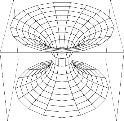
Figure 1: A spatial section $t=const$ of the wormhole (1) (one dimension suppressed). The coordinate $l$ labels the proper distance to the throat along “radial” directions. Surfaces of constant $l$ have area $4\pi r^{2}(l)$ (shown here as circles of circumference $2\pi r(l)$). As one approaches $l=\pm\infty$, the location of the two distinct asymptotic infinities, the circumference of the circles approaches $2\pi|l|$, the geometry becomes flat.

III Wormholes supported by a k-field

One can draw two different conclusions from the fact that only exotic matter may be able to support a wormhole. If one assumes that all matter forms satisfy the above mentioned energy conditions, then our previous result excludes wormholes from general relativity. On the other hand, if one insists upon the existence of wormholes, it follows that the matter that threads them has to be “exotic”. Let us point out that, to our knowledge, there is no reason why all matter forms should satisfy the null, weak and strong energy conditions. In fact, recent indications that the universe is currently accelerating Supernova directly imply that the strong energy condition is violated in nature, by what seems to be acting as a non-vanishing positive cosmological constant. The weak energy condition is violated by a negative cosmological constant, and the study of spaces with such a negative cosmological constant has recently attracted significant attention (see references to Maldacena ). Finally a scalar field with non-linear kinetic terms, a k-field, can basically violate any desired energy condition ArMu . One of the purposes of this paper is to show that, at least in principle, a simple k-field may indeed support wormholes in general relativity. It turns out, that the Lagrangian we are going to consider respects the arguably only physically motivated energy condition, the requirement that the energy-momentum current $T^{\beta}{}_{\alpha}u^{\alpha}$ measured by an observer with arbitrary four velocity $u^{\alpha}$ be non-spacelike.

A k-field is a scalar field $\varphi$ minimally coupled to Einstein gravity. By definition, its action is given by

$$S[g_{\alpha\beta},\varphi,\psi_{m}]=\int d^{4}x\sqrt{-g}\left[-\frac{R}{4}+p(X)\right]+S_{m}[g_{\alpha\beta},\psi_{m}].$$ (7)

Here, the k-field Lagrangian $p(X)$ is an arbitrary function of the squared scalar field gradient,

$$X\equiv\frac{1}{2}g^{\alpha\beta}\nabla_{\alpha}\varphi\nabla_{\beta}\varphi,$$ (8)

which for a static, spherically symmetric configuration is negative, $X=-\frac{1}{2}(\varphi^{\prime})^{2}$. For simplicity we assume that the k-field Lagrangian $p$ only depends on the squared gradient $X$ and not on the k-field $\varphi$ itself. Therefore, the theory is symmetric under constant shifts of the field $\varphi\to\varphi+\epsilon$ and the corresponding current conservation yields the equation of motion of the k-field,

$$\nabla_{\alpha}\left(p_{,X}\nabla^{\alpha}\varphi\right)=0,$$ (9)

where $,X$ denotes a derivative with respect to $X$. The action (7) can be regarded as the simplest generic phenomenological way of providing a microscopic description of the unknown matter that supports a wormhole. We assume that the field only couples to Einstein gravity, and not to additional matter fields $\psi_{m}$.

The energy-momentum tensor of the k-field is given by functional differentiation of the k-field action

$$T_{\alpha\beta}\equiv\frac{2}{\sqrt{-g}}\frac{\delta S}{\delta g^{\alpha\beta}}=\frac{dp}{dX}\nabla_{\alpha}\varphi\nabla_{\beta}\varphi-p\,g_{\alpha\beta}.$$ (10)

If the scalar field gradient is space-like (as is the case in a static field configuration) it can be cast in the form $T_{\alpha\beta}=(\rho-\tau)\,n_{\alpha}n_{\beta}-p\,g_{\alpha\beta}$, where $n_{\alpha}$ is a space-like unit vector pointing in the direction of the field gradient,

$$\tau=2X\frac{dp}{dX}-p$$ (11)

is the radial tension, $\rho=-p$ is the energy density and $p$ is the pressure as defined in (3). Notice that, unlike in a situation where the field gradient is time-like ArMu , the energy-momentum tensor does not have perfect fluid form. The k-field equation of motion (9) can be derived both by functional differentiation of the k-field action or by requiring the energy momentum tensor to be covariantly conserved. For a static, spherically symmetric field configuration, the field equation is given by the “energy conservation” law (5).

The different properties of a wormhole severely restrict the possible Lagrangians $p(X)$ which may support it. According to (6), the null energy condition has to be violated at the throat of the wormhole. Using the properties of the k-field energy momentum tensor, one finds that $\tau+p$ should be positive at $l=0$ and hence there should exist an $X_{T}$, the value of $X$ at the throat, such that

$$\frac{dp}{dX}\Big{|}_{X_{T}}<0.$$ (12)

On the other hand, the requirement of asymptotic flatness also yields important information about the form of the pressure $p$ at infinity. The gravitational field of any isolated source in asymptotically flat spacetime can be expanded in multipole moments. If the source is static and spherically symmetric only monopole moments contribute to the gravitational field, and there exists then a coordinate system where the metric admits an asymptotic expansion of the form Thorne

$$ds^{2}=\left(1+\frac{\phi_{1}}{r}+\frac{\phi_{2}}{r^{2}}+\cdots\right)dt^{2}-\left(1-\frac{\psi_{1}}{r}-\frac{\psi_{2}}{r^{2}}-\cdots\right)\left[dr^{2}+r^{2}d\Omega^{2}\right].$$ (13)

Of course, the k-field cannot be considered as a localized (finite-size) source. We assume that the k-field decays sufficiently fast at infinity, in such a way that the expansion (13) still applies. Plugging the above metric expansion coefficients into Einstein’s field equations (we shall not write them down here), one can derive analogous expansions for $p$ and $\tau$,

$$p = -\frac{3\psi_{1}^{2}+8\psi_{2}}{8\,r^{4}}+\mathcal{O}(r^{-5})$$

$$\tau = \frac{\phi_{1}-\psi_{1}}{2\,r^{3}}-\frac{4\phi_{1}^{2}-8\phi_{2}-2\phi_{1}\psi_{1}+5\psi_{1}^{2}+8\psi_{2}}{8\,r^{4}}+\mathcal{O}\left(r^{-5}\right).$$

Substituting these expansions into the field equation of motion in these coordinates, one finds $\phi_{1}=\psi_{1}$ (as appropriate for a mass term) and $2\phi_{2}=\psi_{1}^{2}$. Therefore,

$$p=-\frac{3\psi_{1}^{2}+8\psi_{2}}{8\,r^{4}}+\mathcal{O}(r^{-5})=\tau+\mathcal{O}(r^{-5}).$$ (14)

At infinity both pressure and radial tension vanish and in the asymptotic limit $r\to\infty$ the ratio of the pressure to the radial tensor tends to 1. We conclude that there should exist an $X_{\infty}$, the asymptotic value of $X$ as $l\to\infty$, where

$$p(X_{\infty})=0,\quad\tau(X_{\infty})=2X_{\infty}\cdot p_{,X}(X_{\infty})=0$$ (15)

and such that, around $X_{\infty}$,

$$\frac{p(X_{\infty}+\Delta X)}{\tau(X_{\infty}+\Delta X)}\approx\frac{p_{,X}(X_{\infty})}{\tau_{,X}(X_{\infty})}=1.$$ (16)

We will argue below that $\tau_{,X}$ should be non-zero between $X_{\infty}$ and $X_{T}$. Then, in order for (16) to be satisfied, $p_{,X}(X_{\infty})$ should be also different from zero. Therefore, it follows from (15) that $X_{\infty}=0$, and thus, around the origin

$$p=\tau\approx c\cdot X,$$ (17)

where $c$ is an arbitrary non-zero coefficient which can be chosen to be $\pm 1$ by a field redefinition. Hence, up to a sign, the k-field behaves at infinity as a massless scalar field. This is consistent with the pressure decaying as $1/r^{4}$ in the limit $r\to\infty$, which corresponds to a $1/r$ decay of the field $\varphi$ at infinity. Finally, as pointed out above, a well defined field equation of motion requires

$$\tau_{,X}\neq 0\quad\mathrm{for}\quad X_{T}\leq X\leq X_{\infty}=0.$$ (18)

The reason is that the points where $\tau_{,X}=0$ are barriers over which the field equation of motion (5) cannot be integrated, so that a continuous field configuration interpolating between $X_{T}$ and $X_{\infty}$ requires $\tau_{,X}$ to be non-zero within that interval.

Conditions (12), (17) and (18) essentially determine the form of the Lagrangian $p$ (as illustrated in Figure 2). Around the origin $p$ must be linear and, in addition, there must exist a point $X_{T}$ where the slope of $p$ is negative. Suppose that $p\approx X$ around the origin. Then there must exist a local minimum of $X_{*}$ between $X_{T}$ and $X=0$ where $p_{,X}=0$. At the minimum $\tau_{,X}(X_{*})\equiv 2X_{*}\,p_{,XX}\,(X_{*})$ is negative, whereas at the origin $\tau_{,X}(0)=1$ is positive. By continuity there is a point $X_{**}$ where $\tau_{,X}$ is zero, violating condition (18). We are forced to choose $p\approx-X$ around $X_{\infty}=0$. An analogous argument implies that the function $p$ cannot have a local maximum, so we conclude that $p(X)$ should be a monotonically decreasing function which is linear at the origin. The simplest function which satisfies this criterion is $p=-X$.

Figure 2: Possible forms of the Lagrangian $p$. It must have a negative slope at $X_{T}$, it must be linear around the origin but because of (18), it cannot have local maxima or minima. Thus, $p$ has to be a monotonically decreasing function of $X$ with a negative slope at the origin.

IV Wormhole solutions

Our previous analysis has determined that $p=-X$ is the simplest Lagrangian which may allow a wormhole solution. From now on, we shall concentrate on this form of the Lagrangian. Notice that for a conventional massless scalar field $p=X$. Hence, the field we are considering is a massless field with a reversed sign kinetic term. As long as the effect of the field on gravity can be ignored, the overall sign of the matter Lagrangian is a matter of convention. In particular, in any given gravitational background the equation of motion of such a field is the same as the one of a conventional massless scalar, $\nabla^{\alpha}\nabla_{\alpha}\varphi=0$. It is the way the field couples to gravity that determines the sign of the Lagrangian. If the scalar field couples only to gravity, this sign can be chosen at will, as long as this does not yield any inconsistency.

Static, spherically symmetric solutions of Einstein’s equations minimally coupled to a conventional massless scalar field have been repeatedly discovered in the literature Fisher . Particularly useful for our purposes are the solutions as presented by Wyman (see also AgneseLaCamera ):

$$ds^{2}=e^{-2m/\tilde{r}}dt^{2}-e^{2m/\tilde{r}}\left(\frac{\eta/\tilde{r}}{\sinh(\eta/\tilde{r})}\right)^{4}d\tilde{r}^{2}-e^{2m/\tilde{r}}\left(\frac{\eta/\tilde{r}}{\sinh(\eta/\tilde{r})}\right)^{2}\tilde{r}^{2}d\Omega^{2},$$ (19)

where $\eta^{2}=m^{2}+q^{2}$ and $q$ is defined by the form of the scalar field solution

$$\varphi=\frac{q}{\tilde{r}}.$$ (20)

These solutions are characterized by two integration constants, a mass $m$ and a “charge” $q$. Because the scalar field solution (20) is proportional to $q$ and the energy-momentum tensor (10) is quadratic in $\varphi$, a real $q$ describes a conventionally coupled scalar field, while a purely imaginary $q$ is equivalent to considering a field with a negative kinetic term. For an ordinary coupling ($q^{2}>0$) the above solutions describe a spacetime with a naked singularity at $\tilde{r}=0$. In fact, after a coordinate transformation, (19) can be cast in the form

$$ds^{2}=\left(1-\frac{2\eta}{r}\right)^{m/\eta}dt^{2}-\left(1-\frac{2\eta}{r}\right)^{-m/\eta}dr^{2}-\left(1-\frac{2\eta}{r}\right)^{1-m/\eta}r^{2}d\Omega^{2},$$ (21)

where one sees that the would-be Schwarzschild horizon has shrunk to a point at $r=2\eta$. If the charge vanishes, $q=0$, equation (21) obviously reduces to the Schwarzschild metric.

If $\eta^{2}=m^{2}+q^{2}$ itself is negative, the metric (21) is not well defined. Of course, $\eta^{2}$ can be negative only if $q$ is purely imaginary (we assume the mass $m$ to be real.) This is physically equivalent to a real scalar field whose kinetic term has the opposite sign, which is precisely the coupling we are interested in. In what follows, we assume that both $\eta^{2}$ and $q^{2}$ are negative. By a change of radial coordinates, the metric (19) can be rewritten as

$$ds^{2}=e^{-2m/\tilde{r}}dt^{2}-e^{2m/\tilde{r}}\left[dr^{2}+(r^{2}-\eta^{2})\,d\Omega^{2}\right],$$ (22)

where the old coordinate $\tilde{r}$ is implicitly expressed in terms of the new coordinate $r$ by the relation

$$\sin^{2}\left(\frac{|\eta|}{\tilde{r}}\right)=\frac{-\eta^{2}}{r^{2}-\eta^{2}},$$ (23)

and the explicit functional dependence $\tilde{r}(r)$ is determined by the requirements of continuity and differentiability. The metric (22) was first discovered in a different coordinate system in Ellis (see also Bronnikov ), and classical scattering in such a geometry has been studied in ChetouaniClement .

Although we shall not cast (22) in proper distance coordinates, it is quite clear that it describes a traversable wormhole. Due to the presence of the $-\eta^{2}$ term, the coordinate $r$ may take values in the range $-\infty\leq r\leq\infty$. The form of $|\eta|/\tilde{r}$ as a function of $r$ is shown in Figure 3. The function $\exp(-2m/\tilde{r})$ is finite everywhere and in particular, the metric (22) does not contain any horizon. In the limit $r\to\infty$, $\exp(-2m/\tilde{r})=1-2m/r+\mathcal{O}(r^{-2})$, and in the limit $r\to-\infty$, $\exp(-2m/\tilde{r})\to\exp(-2\pi m/|\eta|)(1-2m/r+\mathcal{O}(r^{-2}))$. Hence, the spatial sections of (22) contain two asymptotically flat regions and the masses of the wormhole as observed in those regions are $m$ and $-m\exp(\pi m/|\eta|)$ respectively. Notice that the two masses have opposite sign. In addition, because the redshift function is not symmetric under reflections $r\to-r$, clocks tick at different rates in both asymptotic regions and a photon emitted at $r=\infty$ will appear to be blue shifted at $r=-\infty$. The $r$ dependence of the scalar field also has the form of Figure 3. The scalar field solutions is proportional to $q$ and that is the reason why it can be interpreted as a scalar charge (this identification will be made more precise below.)

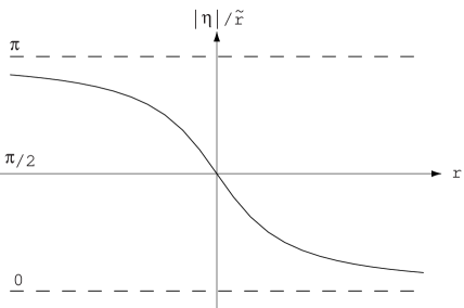
Figure 3: The form of $|\eta|/\tilde{r}$ as a function of the coordinate $r$.

The zero mass wormhole solutions have a remarkably simple form. Setting $m=0$ in (22) and using (20) to compute $p=-\frac{1}{2}(\nabla\varphi)^{2}$ one gets

$$ds^{2} = dt^{2}-dl^{2}-(l^{2}-q^{2})\,d\Omega^{2},$$ (24a)

$$p = \tau=\frac{1}{2}\frac{-q^{2}}{(l^{2}-q^{2})^{2}}.$$ (24b)

Recall that $q^{2}$ is negative for the solutions under consideration, that is, the pressure and radial tension are positive, in agreement with the fact that $p=-X>0$. The reader can easily verify that, indeed, (24) satisfy Einstein’s field equations (4). The static metric (24a) has the wormhole form (1). Its spatial sections $t=const$ contain two asymptotically flat regions at $l=\pm\infty$. The minimal area of a $l=const$ surface occurs at $l=0$, and is given by $-4\pi q^{2}$. The redshift function is constant everywhere, and in particular, there are no tidal forces which could prevent the passage of a person through the wormhole if $|q|$ is sufficiently big. The metric in (24) is in fact the simplest traversable wormhole geometry one may think of.

Suppose that observers living in (24) were able to measure the value of the scalar field. They would realize that it obeys the equation $\Delta\varphi\propto(r^{2}\varphi^{\prime})^{\prime}=0$. By computing the flux of the field gradient through surfaces of constant $l$, they would conclude that this flux is independent of the value of $l$ and is given by $4\pi|q|$. If these observers did not have enough resolving power to explore lengths of size $|q|$, they would hence arrive at the conclusion that there is a scalar source of charge $|q|$ sitting within $l<q$. However, there is no scalar source present. In reality there is a sourceless incoming flux which originates at $l=-\infty$, passes through the wormholes mouth at $l=0$, and emerges again for $l>0$ as an outgoing flux reaching $l=\infty$. This is one example of Wheeler’s “charge without charge” Wheeler .

V Wormhole stability

One of the advantages of a microscopic description of the matter that threads a wormhole is that such a description allows us to address issues which would have not been treatable otherwise. The stability of wormholes is such an example. In the following, we analyse in first order perturbation theory the stability of the wormhole solutions we have previously discussed. Because of their extreme simplicity, we concentrate on the zero mass solutions (24), although we shall later argue that solutions with sufficiently small $m$ are also stable. Our analysis closely resembles an analogous investigation in ReggeWheeler (see also Vishveshwara and Zerilli ), although we will not work in Schwarzschild coordinates but in the proper distance coordinate system (1), where all metric coefficients are regular functions.

The strategy is the following. We introduce metric and field perturbations, $g_{\alpha\beta}\to g_{\alpha\beta}+h_{\alpha\beta}$, $\varphi\to\varphi+\delta\varphi$ around the background solution (24). Linearizing Einstein’s equations one gets a closed system of equations for the metric and field perturbations, $\delta G_{\alpha\beta}=\delta T_{\alpha\beta}$. If these equations admit spatially well behaved solutions, that is, perturbations that decay sufficiently fast at spatial infinity, which grow exponentially in time, our background solutions are unstable. The symmetries of the background solution allow us to simplify the analysis of its perturbations. Due to the staticity of the background, we can decompose the perturbations into Fourier modes proportional to $e^{i\omega t}$ which do not couple to each other in the linear regime. Similarly, because the background is spherically symmetric, it is convenient to decompose the perturbations into spherical harmonics $Y_{Lm}(\theta,\phi)$ and its derivatives, and again, the symmetry under rotations makes possible to consider only perturbations with azimuthal eigenvalue $m=0$. Finally, the inversion symmetry of the background ($l\to l$, $\theta\to\pi-\theta$, $\phi\to\pi+\phi)$ allows us to consider perturbations of definite parity $P$ under inversion. Perturbations of “electric” (or even) type have $P=(-1)^{L}$ and perturbations of “magnetic” (or odd) type have parity $P=(-1)^{L+1}$. In linearized perturbation theory, perturbations with different “quantum numbers” $\omega$, $L$ and $P$ decouple from each other.

In Regge-Wheeler gauge, the electric type metric perturbations (denoted by $\mathrm{(e)}$) are

$$h^{\mathrm{(e)}}_{\alpha\beta}=\left(\begin{array}[]{cccc}H_{0}(l)&H_{1}(l)&0&0\\ H_{1}(l)&H_{2}(l)&0&0\\ 0&0&r^{2}K(l)&0\\ 0&0&0&r^{2}K(l)\sin^{2}\theta\end{array}\right)P_{L}(\cos\theta)e^{i\omega t}.$$ (25)

The indices $\alpha$ and $\beta$ run over the coordinates $t,l,\theta$ and $\phi$. The Legendre polynomial $P_{L}$ is the $m=0$ spherical harmonic $Y_{L\,m}$. As previously mentioned, the time and angular dependence of the perturbations has been explicitly separated and hence, only their dependence on the $l$ variable remains to be determined. Similarly, the magnetic perturbations (denoted by the label $\mathrm{(m)}$) are

$$h^{\mathrm{(m)}}_{\alpha\beta}=\left(\begin{array}[]{cccc}0&0&0&h_{0}(l)\\ 0&0&0&h_{1}(l)\\ 0&0&0&0\\ h_{0}(l)&h_{1}(l)&0&0\end{array}\right)\sin\theta\frac{d}{d\theta}P_{L}(\cos\theta)e^{i\omega t},$$ (26)

so that there are 4 electric and 2 magnetic metric perturbation functions in total. The remaining 4 functions needed to complete the most general metric perturbation are zero in Regge-Wheeler gauge. The scalar field perturbations are

$$\delta\varphi^{\mathrm{(e)}}=\delta\varphi^{\mathrm{(e)}}(l)P_{L}(\cos\theta)e^{i\omega t}\quad\rm{and}\quad\delta\varphi^{\mathrm{(m)}}=0,$$ (27)

and in particular, because a scalar field is a scalar under parity transformations, there are no magnetic type field perturbations. It turns out that both for electric and magnetic perturbations, one can derive an equation for a single perturbation variable $Q^{\rm(e,m)}$. The equation has the form of a Schrödinger eigenvalue problem

$$-\frac{d^{2}}{dl^{2}}Q^{{\rm(e,m)}}+V_{L}(l)Q^{{\rm(e,m)}}=\omega^{2}Q^{{\rm(e,m)}},$$ (28)

where the potential $V_{L}$ also depends on the angular momentum $L$ of the perturbations. Solutions of this equation with negative $\omega^{2}$ correspond to exponentially growing and decaying modes. Hence, our task consists in verifying whether (28) admits spatially well behaved solutions of negative $\omega^{2}$ . Because the potential goes to 0 as $l\to\pm\infty$, this is equivalent to verifying whether $V_{L}$ admits any bound state, that is, an eigenfunction of negative energy.

Electric perturbations

For these perturbations, the relevant linearized equations read (dropping the (e)-label)

$$[L(L+1)+2]H_{2}+2H_{2}^{\prime}rr^{\prime}+(L+2)(L-1)K-6K^{\prime}rr^{\prime}-2K^{\prime\prime}r^{2}=r^{2}\varphi^{\prime}\delta\varphi^{\prime}$$ (29a)

$$L(L+1)H_{1}-2i\omega Krr^{\prime}+2i\omega H_{2}rr^{\prime}-2i\omega K^{\prime}r^{2}=i\omega r^{2}\varphi^{\prime}\delta\varphi$$ (29b)

$$2H_{2}-L(L+1)H_{0}+(L+2)(L-1)K+(2H_{0}^{\prime}-2K^{\prime}-4i\omega H_{1})rr^{\prime}-\hskip 56.9055pt$$

$${}-2\omega^{2}Kr^{2}=-r^{2}\varphi^{\prime}\delta\varphi^{\prime}$$ (29c)

$$\frac{dP_{L}}{d\cos\theta}\left[H_{0}r^{\prime}-H_{2}r^{\prime}-H_{0}^{\prime}r+K^{\prime}r+i\omega H_{1}r\right]=-\frac{dP_{L}}{d\cos\theta}r\varphi^{\prime}\delta\varphi$$ (29d)

$$\frac{d^{2}P_{L}}{d(\cos\theta)^{2}}\cdot(H_{0}-H_{2})=0$$ (29e)

$$-\omega^{2}\delta\varphi-\delta\varphi^{\prime\prime}-2\frac{r^{\prime}}{r}\delta\varphi^{\prime}+\frac{L(L+1)}{r^{2}}\delta\varphi-\frac{1}{2}(H_{0}^{\prime}+H_{2}^{\prime}-2K^{\prime}-2i\omega H_{1})\,\varphi^{\prime}=0,$$ (29f)

where the background equations (4) have been used. The cases $L=0$, $L=1$ and $L\geq 2$ require separate treatment. If $L\geq 2$ equation (29e) yields $H_{0}=H_{2}$. Then, equation (29d) can be used to express the metric perturbations of the linearized scalar field equation (29f) in terms of the field perturbation $\delta\varphi$. The latter equation reduces to (28), where the potential is given by

$$V_{L}(l)=\frac{L(L+1)}{r^{2}}-3\frac{r^{\prime\prime}}{r}=\frac{L(L+1)\,l^{2}-q^{2}(L^{2}+L-3)}{(l^{2}-q^{2})^{2}},$$ (30)

and $Q^{\rm(e)}\equiv r\delta\varphi$. For $L\geq 2$ the potential is positive everywhere. Because positive potentials do not admit bound states ($E<0$), it is clear that all electric modes with $L\geq 2$ are stable.

Although for $L=1$ the linearized equation (29e) identically vanishes, it is still possible to choose a gauge where $H_{0}=H_{2}$, since $L=1$ perturbations have fewer free functions than $L\geq 2$ perturbations. The potential is thus still given by (30), but in the latter case it has a negative minimum at $l=0$. The $L=1$ Schrödinger equation (28) can be solved exactly for $\omega^{2}=0$. One solution is Meijer’s G-function $G^{11}_{22}\left(1-l^{2}/q^{2}\,\big{|}{\tiny\begin{array}[]{cc}1/2&2\\ 3/2&-1/2\end{array}}\!\right)$ GraRyz . This solution is shown in Figure 4. It is even, decays at infinity and it has no nodes. Hence it is the ground state of the potential $V_{1}$ MorseFeshbach . In particular there are no spatially well-behaved solutions at infinity with $\omega^{2}<0$, and the $L=1$ mode is stable.

The most general metric perturbation for $L=0$ (spherically symmetric) has fewer free functions than for $L\geq 1$. In fact, it is possible to choose a gauge where $K=H_{1}=0$. Using the linearized equations (29a), (29b) and (29), equation (29f) can be cast in the form (28), where the potential is given by

$$V_{0}(l)=\frac{r^{\prime\prime}}{r}+2\frac{r^{\prime\prime}}{r\,r^{\prime}{}^{2}}=\frac{2\,q^{4}-3\,q^{2}\,l^{2}}{l^{2}\,(l^{2}-q^{2})^{2}}.$$ (31)

The latter potential is everywhere positive, and hence, equation (28) does not admit any $\omega^{2}<0$ solutions. Electric spherically symmetric perturbations are also stable.

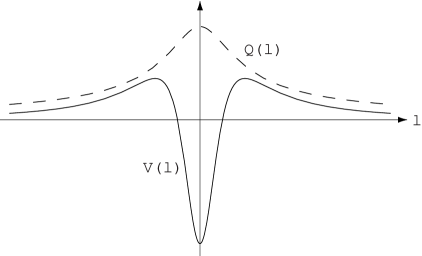
Figure 4: The $L=1$ potential for even perturbations (continuous) and its ground state (dashed).

Magnetic perturbations

The only non-trivial linearized Einstein field equations it suffices to consider are the $x\phi$ and $l\phi$ respectively,

$$(h_{1}^{\prime}-i\omega h_{0})\frac{d^{2}P_{L}}{d(\cos\theta)^{2}}=0$$ (32a)

$$-\omega^{2}h_{1}-i\omega h_{0}^{\prime}+2i\omega\frac{r^{\prime}}{r}h_{0}+2\frac{r^{\prime\prime}}{r}h_{1}+\frac{(L+2)(L-1)}{r^{2}}h_{1}=2\,\varphi^{\prime}{}^{2}\,h_{1}.$$ (32b)

There are no magnetic perturbations with $L=0$. For $L=1$ equation (32a) does not contain significant information and the remaining equation, (32b), provides a relation between $h_{1}$ and $h_{0}$ that allows us to gauge these perturbations away. For $L\geq 2$ equation (32a) yields the relation $h_{1}^{\prime}=i\omega h_{0}$, which when substituted into (32b) allows us to put it in the form (28), where $Q^{\rm(m)}\equiv h_{1}/r$ and the potential is the same as for electric perturbations, (30). Therefore, $L\geq 2$ magnetic modes are also stable.

Up to now, our discussion has focused on the stability of the zero mass solutions. Because of that, we have only considered time dependent perturbations, i.e on non-zero values of $\omega$. If one studies time-independent $L=0$ perturbations, one has to recover non-zero mass solutions (22) for sufficiently small values of $m$ as time-independent perturbations of the zero-mass solutions. Due to linearity, the time-dependent perturbations around these non-zero mass solutions satisfy, of course, the same perturbation equations (29) and (32). Since these equations do not have any spatially well-behaved growing solution, we conclude that at least for sufficiently small values of $m$ the solutions (22) are also stable. This completes our wormhole stability analysis.

Up to some extent, the stability of the wormhole solutions we have considered was to be expected in the light of the results of GaMu . In that work, it is shown that the speed of propagation of linear perturbations in a cosmological background, $c_{s}$, is given by

$$c_{s}^{2}=\frac{p_{,X}}{\rho_{,X}}.$$ (33)

If the squared speed of happened to be negative, one would anticipate instabilities of the wormhole associated with the exponential growth of short-wavelength modes. Because $c_{s}^{2}=1>0$ in our model, there is no reason to expect those instabilities. However, this argument only addresses the issue partially, since static, spherically symmetric solutions of Einstein’s equations coupled to a canonical field ($c_{s}^{2}=1$) are unstable JetzerScialom . (In the latter case the instability appears in the $L=0$ mode.)

VI Conclusions

Non-canonical scalar field Lagrangians allow the existence of wormhole solutions in general relativity. The conditions of asymptotic flatness and the existence of a wormhole throat essentially force the non-canonical scalar field to be a massless scalar field with a reversed sign Lagrangian. Zero mass wormhole solutions to Einstein’s equations coupled to such a field turn out to be extremely simple and are useful as toy models to explore different aspects of wormhole physics. As a particular application, it is possible to show their stability against linear perturbations analytically. The issue about the physical viability of such a scalar field is yet unsettled, although at the level of our investigation we have not discovered any internal inconsistency. Rather, it turns out that because such a field violates some of the standard energy conditions, cosmological and spherically symmetric solutions of Einstein’s field equations are singularity-free.

Appendix A Stability of Minkowski space

Our work has mainly focused on a massless scalar field described by a Lagrangian $p$ whose sign has been reversed. In other words, we have considered a Lagrangian

$$p=\frac{\kappa}{2}\nabla_{\alpha}\varphi\,\nabla^{\alpha}\varphi$$ (34)

where $\kappa$ is $-1$ instead of $+1$. One of the main objections against such an assumption is that for such a scalar field, Minkowski space should be unstable. Indeed, on general grounds one expects small scalar field fluctuations to radiate positive energy in form of gravitational waves, making the negative energy density of the initial field fluctuations even more negative and leading to a complete instability of the vacuum. Let us verify whether one observes this kind of behavior in perturbation theory. In order to establish the difference with respect to an ordinary scalar field, we will keep $\kappa$ as a free parameter. Consider perturbations of Minkowski space to second order,

$$g_{\alpha\beta}=\eta_{\alpha\beta}+h^{(1)}_{\alpha\beta}+h^{(2)}_{\alpha\beta}+\cdots,$$

where the notation should be obvious, and consider equally second order perturbations of of a constant massless scalar field,

$$\varphi=\varphi^{(0)}+\varphi^{(1)}+\varphi^{(2)}+\cdots,$$

where $\partial_{\alpha}\varphi^{(0)}=0$. To first order in perturbation theory, the Einstein and Klein-Gordon equations are

$$\eta^{\mu\nu}\partial_{\mu}\partial_{\nu}\left(h^{(1)}_{\alpha\beta}-\frac{1}{2}\eta_{\alpha\beta}h^{(1)}\right) = 0,$$ (35)

$$\eta^{\mu\nu}\partial_{\mu}\partial_{\nu}\varphi^{(1)} = 0.$$ (36)

Upon gauge fixing, the first of the equations describes gravitational waves propagating in Minkowski spacetime, while the second one describes scalar field waves propagating in the same background. Notice that these equations are the same regardless of $\kappa$ in (34). At this level, both signs are equally valid.

Consider then the second order Einstein equations,

$$\eta^{\mu\nu}\partial_{\mu}\partial_{\nu}\left(h^{(2)}_{\alpha\beta}-\frac{1}{2}\eta_{\alpha\beta}h^{(2)}\right)=4\kappa\left(\partial_{\alpha}\varphi^{(1)}\partial_{\beta}\varphi^{(1)}-\frac{1}{2}\eta_{\alpha\beta}\partial_{\gamma}\varphi^{(1)}\partial^{\gamma}\varphi^{(1)}\right)-2G^{(2)}(h^{(1)}).$$ (37)

The sign of the first term on the right hand is determined by the conventional/unconventional coupling of the massless scalar field to gravity and the second term on the right hand side contains all terms of the Einstein tensor quadratic in the first order perturbations $h^{(1)}$. Thus, the right hand side of the above equation describes how the first order scalar field and gravitational waves respectively back-react on the background geometry. Whereas the gravitational wave back-reaction is the same for both signs of the scalar field coupling, the scalar field wave back-reaction on the metric does depend to this order on the sign of the energy momentum tensor, as expected. The Klein-Gordon equation to second order

$$\eta^{\mu\nu}\partial_{\mu}\partial_{\nu}\varphi^{(2)}=-\partial_{\alpha}\left(h^{(1)}{}^{\alpha\beta}\partial_{\beta}\varphi^{(1)}-\frac{1}{2}h^{(1)}\partial^{\alpha}\varphi^{(1)}\right)$$

describes how first order scalar and gravitational waves generate second order field perturbations. For given perturbations, it is the same for both signs of the scalar field coupling.

Suppose that we solve equation (37) in a given background of first order scalar waves (assume for the sake of the argument that there are no gravitational waves.) The solution is given by the convolution of the (known) source terms in the right hand side with the appropriate retarded Green’s function. In particular, the solutions for both values of $\kappa$ differ only by a sign. If the solution is well behaved for $\kappa=1$, it is also well behaved for $\kappa=-1$. Thus, at second order there is not yet any evidence that $\kappa=+1$ is preferable to $\kappa=-1$. It seems that if we want to single out $\kappa=1$ as the preferred choice of the scalar field coupling, we have to go to higher orders.

Due to the structure of the perturbation equations, even if we proceeded to higher orders it would be difficult to discover why $\kappa=+1$ is essentially different from $\kappa=-1$ (as in the “analogous” system of two coupled scalar fields, one with a conventional, the other with an unconventional kinetic term.) At this point let us try a non-perturbative analysis and point out that even the conventional coupling $\kappa=1$ leads to instabilities. Consider for that purpose an homogeneous spatially flat universe filled by a canonical scalar field,

$$ds^{2}=dt^{2}-a(t)^{2}\left[dr^{2}+r^{2}d\Omega^{2}\right].$$

It is known that the solution of Einstein’s and Klein-Gordon equations in such a spacetime is given by

$$a(t) \propto |t|^{1/3}$$

$$\left(\frac{d\varphi}{dt}\right)^{2} \propto \frac{1}{t^{2}}.$$

This solution has two branches, related to each other by time reversal. For positive times, the universe starts expanding at the big bang singularity at $t=0_{+}$ and approaches Minkowski space at $t=\infty$ (the Hubble parameter $d\log a/dt$ approaches zero). For negative times the universe starts from Minkowski space at $t=-\infty$ and contracts into a “pre-big bang” singularity at $t=0_{-}$. This latter branch implies that a canonical massless scalar field in Minkowski space is “unstable” upon contraction. As a matter of fact, this instability is one of the ideas behind the pre-big bang scenario and reflects nothing else other than the gravitational instability upon collapse of the scalar and gravitational waves around Minkowski spacetime DamourVeneziano we have previously encountered. Notice that an analogous argument applies for $p=-X$, though there is a crucial difference too. In the latter case, the scalar field has a negative energy density, and the spatial sections of the universe have to be negatively curved. Expanding solutions hence asymptotically approach the “Milne universe”, which is just a portion of Minkowski space. On the other hand contracting solutions (the time reversed expanding solutions) originate from Minkowski space and instead of running into a singularity, bounce at a finite value of $a$ and expand again into Minkowski spacetime (this is possible because our field violates the null energy condition VisserMolina ).

References

- (1) M. Visser, Lorentzian Wormholes: From Einstein to Hawking, American Institute of Physics (1995).
- (2) M. Morris and K. Thorne, Wormholes in spacetime and their use for interstellar travel: A tool for teaching general relativity, Am. J. Phys. 56, 395 (1988).
- (3) C. Armendariz-Picon, T. Damour and V. Mukhanov, k-Inflation, Phys. Lett. B458, 209 (1999). C. Armendariz-Picon, V. Mukhanov and P. Steinhardt, Essentials of k-Essence, Phys. Rev. D63, 103510 (2001).
- (4) I. Fisher, Scalar mesostatic field with regard for gravitational effects, Zhurnal Experimental’noj Teoreticheskoj 18, 636 (1948), gr-qc/991100. A. Janis, E. Newman and J. Winicour, Reality of the Schwarzschild Singularity, Phys. Rev. Lett. 20, 878 (1968). M. Wyman, Static spherically symmetric scalar fields in general relativity, Phys. Rev. D24, 839 (1981).
- (5) P. Jetzer and D. Scialom, Dynamical instability of the static real scalar field solitons to the Einstein-Klein-Gordon equations, Phys. Lett. A169, 12 (1992).
- (6) H. Ellis, Ether flow through a drainhole: A particle model in general relativity, J. Math. Phys. 14, 104 (1973).
- (7) K. Bronnikov, Scalar-Tensor Theory and Scalar Charge, Acta Phys. Pol. B4, 251 (1973).
- (8) A. Einstein and N. Rosen, The Particle Problem in the General Theory of Relativity, Phys. Rev. 48, 73 (1935).
- (9) T. Kodama, General-relativistic nonlinear field: A kink solution in a generalized geometry, Phys. Rev. D18, 3529 (1978).
- (10) R. Caldwell, A Phantom Menace?, astro-ph/9908168. A. Schulz and M. White, The Tensor to Scalar Ratio of Phantom Dark Energy Models, Phys. Rev. D64, 043514 (2001).
- (11) C. Hull, de Sitter space in supergravity and M theory, JHEP 0111, 012 (2001).
- (12) S. Hawking and G. Ellis, The large scale structure of spacetime, Cambridge University Press (1973).
- (13) P. Garnavich et al., Supernova Limits on the Cosmic Equation of State, Astrophys. J. 509, 74 (1998). S. Perlmutter, M. Turner and M. White, Constraining dark energy with SNe Ia and large-scale structure, Phys. Rev. Lett. 83, 670 (1999).
- (14) J. Maldacena, The large limit of superconformal field theories and supergravity, Adv. Theor. Math. Phys. 2, 231 (1998). [Int. J. Theor. Phys. 38, 1113 (1998).]
- (15) K. Thorne, Multipole expansions of gravitational radiation, Rev. Mod. Phys. 52, 299 (1980).
- (16) A. Agnese and M. La Camera, Gravitation without black holes, Phys. Rev. D31, 1280 (1985).
- (17) L. Chetouani and G. Clement, Geometrical Optics in the Ellis Geometry, Gen. Rel. Grav. 16, 111 (1984).
- (18) J. Wheeler, Geometrodynamics, Academic Press (1962).
- (19) T. Regge and J. Wheeler, Stability of a Schwarzschild Singularity, Phys. Rev. 108, 1063 (1957).
- (20) C. Vishveshwara, Stability of the Schwarzschild Metric, Phys. Rev. D1, 2870 (1970).
- (21) F. Zerilli, Gravitational Field of a Paricle Falling in a Schwarzschild Geometry Analyzed in Tensor Harmonics, Phys. Rev. D2, 2141 (1970).
- (22) I. Gradshteyn and I. Ryzhik, Table of Integrals, Series, and Products, Academic Press, Inc. (1980).
- (23) P. Morse and H. Feshbach, Methods of Theoretical Physics, McGraw-Hill (1953).
- (24) J. Garriga and V. Mukhanov, Perturbations in k-inflation, Phys. Lett. B458, 219 (1999).
- (25) A. Buonanno, T. Damour and G. Veneziano, Pre-big bang bubbles from the gravitational instability of generic string vacua, Nucl. Phys. B543, 275 (1999).
- (26) C. Molina-Paris and M. Visser, Minimal conditions for the creation of a Friedman-Robertson-Walker universe from a ’bounce’, Phys. Lett. B455, 90 (1999).