Analogue models of and for gravity

Abstract

Condensed matter systems, such as acoustics in flowing fluids, light in moving dielectrics, or quasiparticles in a moving superfluid, can be used to mimic aspects of general relativity. More precisely these systems (and others) provide experimentally accessible models of curved-space quantum field theory. As such they mimic kinematic aspects of general relativity, though typically they do not mimic the dynamics. Although these analogue models are thereby limited in their ability to duplicate all the effects of Einstein gravity they nevertheless are extremely important — they provide black hole analogues (some of which have already been seen experimentally) and lead to tests of basic principles of curved-space quantum field theory. Currently these tests are still in the realm of gedanken-experiments, but there are plausible candidate models that should lead to laboratory experiments in the not too distant future.
PACS: 04.40.-b; 04.60.-m; 11.10.-z; 45.20.-d; gr-qc/0111111.
Keywords: analogue models, general relativity, acoustic horizon.

Plenary talk presented by Matt Visser.
Australasian Relativity Conference.
Perth, Australia, July 2001.
Proceedings to appear in General Relativity and Gravitation.

1 Introduction

Analogue models of (and to some extent for) general relativity have recently become a growth industry [1]. Typically based on various condensed-matter systems, these analogue models are most often used for devising gedanken-experiments that probe the structure of curved-space quantum field theory. More boldly, they seem promising routes to providing real laboratory tests of the foundations of curved-space quantum field theory. (The most spectacular suggestion along these lines is that analogue models may make experimental tests of the Hawking radiation phenomenon a realistic possibility.)

Ideas along these lines have, to some extent, been quietly in circulation almost since the inception of general relativity itself. Walther Gordon (of the Klein–Gordon equation) introduced a notion of “effective metric” to describe the effect of a refractive index on the propagation of light [2]. The Russian school, as epitomized by Landau and Lifshitz, used notions developed in optics to represent gravitational fields in terms of an “equivalent refractive index” [3]. There is an extensive, but largely neglected samizdat literature (of extremely variable quality) that explores these issues. (For an extensive, though still not comprehensive, bibliography see [4].)

The modern revival is due largely to Unruh [5] (and to some extent Moncrief [6]) who in the early eighties considered the use of hydrodynamic analogues, in which sound waves in a flowing fluid are mapped into a suitable scalar field theory in an effective curved spacetime — the “acoustic geometry”. (The precise statement, as will be described more fully below, is that sound in an irrotational inviscid barotropic fluid is identical to a massless minimally coupled scalar field in curved spacetime; and quantized sound [the phonon field] is identical to curved-space quantum field theory.)

The nineties saw considerable work on the nature of Hawking radiation in these analogue models, still largely with the attitude that one was performing gedanken-experiments. It is only now, at the turn of the millennium, that serious consideration is being given to the actual construction of laboratory experiments. Three classes of system stand out as being the most likely to lead to useful experimental probes:

• Acoustics in Bose–Einstein condensates.

• Slow light.

• Quasiparticles in superfluids.

2 Acoustics in BECs

In this mini-survey we will mainly concentrate on acoustics in BECs, and give some feel for where we stand and what the near-term prospects are. Acoustic analogues of black holes are formed by supersonic fluid flow [5, 7]. The flow entrains sound waves and forms a trapped region from which sound cannot escape. The surface of no return, the acoustic horizon, is qualitatively very similar to the event horizon of a general relativity black hole; in particular Hawking radiation (in this case a thermal bath of phonons with temperature proportional to the “surface gravity”) is expected to occur [5, 7]. There are at least three physical situations in which acoustic horizons are known to occur: Bondi–Hoyle accretion [8], the Parker wind [9] (coronal outflow from a star), and supersonic wind tunnels. Recent improvements in the creation and control of Bose–Einstein condensates (see e.g., [10, 11]) have lead to a growing interest in these systems as experimental realizations of acoustic analogs of event horizons. In reference [12] we considered supersonic flow of a BEC through a Laval nozzle (converging-diverging nozzle) in a quasi-one-dimensional approximation. We showed that this geometry allows the existence of a fluid flow with acoustic horizons without requiring any special external potential, and we then studied this flow with a view to finding situations in which the Hawking effect is large. We were able to present simple physical estimates for the “surface gravity” and Hawking temperature, and so to identify an experimentally plausible configuration with a Hawking temperature of order $70$ n K; this figure should be contrasted with the critical condensation temperature which is of the order of $90$ n K. We stress that in present day experiments the actual physical temperature of the condensate, although difficult to measure, is believed to lie well below this critical temperature.

2.1 From Gross–Pitaevskii to hydrodynamics

Bose–Einstein condensates are most usefully described by the nonlinear Schrödinger equation, also called the Gross–Pitaevskii equation, or sometimes the time-dependent Landau–Ginsburg equation:

$$-i\hbar\;\partial_{t}\psi(t,\vec{x})=-{\hbar^{2}\over 2m}\nabla^{2}\psi(t,\vec{x})+\lambda\;||\psi||^{2}\;\psi(t,\vec{x}).$$ (2.1)

(We have suppressed the externally applied trapping potential for algebraic simplicity. For many technical details, and various extensions of the model, see Barceló et al. [13]. That reference also contains an extensive background bibliography.) Now use the Madelung representation [14] to put the Schrödinger equation in “hydrodynamic” form:

$$\psi=\sqrt{\rho}\;\exp(-i\theta\;m/\hbar).$$ (2.2)

Take real and imaginary parts: The imaginary part is a continuity equation for an irrotational fluid flow of velocity $\vec{v}\equiv\nabla\theta$ and density $\rho$; while the real part is a Hamilton–Jacobi equation (Bernoulli equation; its gradient leads to the Euler equation). Specifically:

$$\partial_{t}\rho+\nabla\cdot(\rho\;\nabla\theta)=0.$$ (2.3)

$$\frac{\partial}{\partial t}\theta+{1\over 2}(\nabla\theta)^{2}+{\lambda\;\rho\over m}-{\hbar^{2}\over 2m^{2}}\;{\Delta\sqrt{\rho}\over\sqrt{\rho}}=0.$$ (2.4)

That is, the nonlinear Schrödinger equation is completely equivalent to irrotational inviscid hydrodynamics with a particular form for the enthalpy

$$h=\int{{\mathrm{d}}p\over\rho}={\lambda\;\rho\over m},$$ (2.5)

plus a peculiar derivative self-interaction:

$$V_{Q}=-{\hbar^{2}\over 2m^{2}}\;{\Delta\sqrt{\rho}\over\sqrt{\rho}}.$$ (2.6)

The equation of state for this “quantum fluid” is calculated from the enthalpy

$$p={\lambda\;\rho^{2}\over 2m}.$$ (2.7)

The corresponding speed of sound is

$$c_{s}^{2}={{\mathrm{d}}p\over{\mathrm{d}}\rho}={\lambda\;\rho\over m}.$$ (2.8)

2.2 Acoustic metric

To now extract a Lorentzian geometry, linearize around some background. In the low-momentum limit it is safe to neglect $V_{Q}$. It is a by now standard result that the phonon is a massless minimally-coupled scalar that satisfies the d’Alembertian equation in the effective (inverse) metric [5, 7, 13]

$$g^{\mu\nu}(t,\vec{x})\equiv{\rho_{0}\over c_{s}}\left[\matrix{-1&\vdots&-v_{0}\cr\cdots\cdots&\cdot&\cdots\cdots\cdots\cdots\cr-v_{0}&\vdots&(c_{s}^{2}\;{\mathbf{I}}-v_{0}\otimes v_{0})\cr}\right].$$ (2.9)

Here

$$c_{s}^{2}\equiv{\lambda\;\;\rho_{0}\over m};\qquad\qquad v_{0}={\nabla\theta_{0}}.$$ (2.10)

It cannot be overemphasized that low-momentum phonon physics is completely equivalent to (scalar) quantum field theory in curved spacetime. That is, everything that theorists have learned about curved space QFT can be carried over to this acoustic system, and conversely acoustic experiments can in principle be used to experimentally investigate curved space QFT. In particular, it is expected that acoustic black holes (dumb holes) will form when the condensate flow goes supersonic, and that they will emit a thermal bath of Hawking radiation at a temperature related to the physical acceleration of the condensate as it crosses the acoustic horizon [5, 7, 13, 15]. For completeness we mention that the metric is

$$g_{\mu\nu}(t,\vec{x})\equiv\;{\rho_{0}\over c_{s}}\;\left[\matrix{-(c_{s}^{2}-v_{0}^{2})&\vdots&-{\vec{v}}_{0}\cr\cdots\cdots\cdots\cdots&\cdot&\cdots\cdots\cr-{\vec{v}}_{0}&\vdots&\mathbf{I}\cr}\right],$$ (2.11)

so the space-time interval can be written 

$${\mathrm{d}}s^{2}={\rho_{0}\over c_{s}}\;\left[-c_{s}^{2}\;{\mathrm{d}}t^{2}+||{\mathrm{d}}\vec{x}-\vec{v}_{0}\;{\mathrm{d}}t||^{2}\right].$$ (2.12)

The low-momentum phonon physics looks completely Lorentz invariant. (This is an acoustic Lorentz invariance mind you, with the speed of sound doing duty for the speed of light [7].)

2.3 Hawking effect

2.3.1 Laval nozzle

A general problem with the experimental construction of acoustic horizons is that many of the background fluid flows so far studied seem to require very special fine-tuned forms for the external potential. (See e.g., the Schwarzschild-like geometry in reference [16].) In this respect a possible improvement toward the realizability of acoustic horizons is the construction of a flow in a trap which “geometrically constrains” the flow in such a way as to replace the need for a special external potential. An example of such a geometry is the so called Laval nozzle (converging-diverging nozzle). In particular we shall consider a pair of Laval nozzles; this provides a system which includes a region of supersonic flow bounded between two subsonic regions.

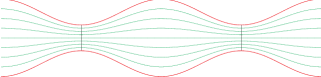
Figure 1: A pair of Laval nozzles: The second constriction is used to bring the fluid flow back to subsonic velocities.

Consider such a nozzle pointing along the $z$ axis. Let the cross sectional area be denoted $A(z)$. We apply, with appropriate modifications and simplifications, the calculations of references [12] and [16]. The crucial approximation is that transverse velocities (in the $x$ and $y$ directions) are small with respect to velocity along the $z$ axis. Then, assuming steady flow, we can write the continuity equation in the form

$$\rho(z)\;A(z)\;v(z)=J;\qquad J=\hbox{constant.}$$ (2.13)

The Euler equation (which we simplify by excluding external forces ${\mathrm{d}}\Phi/{\mathrm{d}}z$, and excluding internal viscous friction $f_{v}$) reduces to

$$\rho\;v\;{{\mathrm{d}}v\over{\mathrm{d}}z}=-{{\mathrm{d}}p\over{\mathrm{d}}z}.$$ (2.14)

Finally, we assume a barotropic equation of state $\rho=\rho(p)$, and define $X^{\prime}={\mathrm{d}}X/{\mathrm{d}}z$. Then continuity implies

$$\rho^{\prime}=-\rho\;{(Av)^{\prime}\over(Av)}=-\rho\left[{A^{\prime}\over A}+{v^{\prime}\over v}\right]=-\rho\left[{A^{\prime}\over A}+{a\over v^{2}}\right],$$ (2.15)

while Euler implies

$$\rho\;a=-{{\mathrm{d}}p\over{\mathrm{d}}\rho}\;\rho^{\prime}.$$ (2.16)

Defining the speed of sound by $c^{2}={\mathrm{d}}p/{\mathrm{d}}\rho$, and eliminating $\rho^{\prime}$ between these two equations yields a form of the well-known “nozzle equation”

$$a=-{v^{2}\;c^{2}\over c^{2}-v^{2}}\left[{A^{\prime}\over A}\right].$$ (2.17)

The presence of the factor $c^{2}-v^{2}$ in the denominator is crucial and leads to several interesting physical effects. For instance, if the physical acceleration is to be finite at the acoustic horizon, we need

$$A^{\prime}\;\to\;0.$$ (2.18)

This is a fine-tuning condition that forces the acoustic horizon (technically, the acoustic ergosurface) to form at exactly the narrowest part of the nozzle. (If external body forces and internal friction are not neglected, then there is a precise relationship between these forces and the location of the horizon.) Experience with wind tunnels has shown that the flow will indeed self-adjust (in particular, the location of the acoustic horizon will self-adjust) so as to satisfy this fine tuning. We can now calculate the acceleration of the fluid at the acoustic horizon by adopting L’Hôpital’s rule.

$$a_{H}={-c^{4}_{H}A^{\prime\prime}_{H}/A_{H}\over(c^{2})^{\prime}_{H}-2a_{H}}.$$ (2.19)

Now use the fact that

$$(c^{2})^{\prime} \equiv {{\mathrm{d}}^{2}p\over{\mathrm{d}}\rho^{2}}\;\rho^{\prime}=-\rho\;{{\mathrm{d}}^{2}p\over{\mathrm{d}}\rho^{2}}\;{(A\;v)^{\prime}\over A\;v}\to-\rho_{H}\;{{\mathrm{d}}^{2}p\over{\mathrm{d}}\rho^{2}}\bigg{|}_{H}\;\left[{a_{H}\over c_{H}^{2}}\right].$$ (2.20)

Therefore

$$a_{H}^{2}={c^{4}\;A^{\prime\prime}/A\over 2+\rho({\mathrm{d}}^{2}p/{\mathrm{d}}\rho^{2})/c^{2}}\bigg{|}_{H}.$$ (2.21)

That is

$$a_{H}=\pm{c^{2}\over\sqrt{2A}}\;\left.\sqrt{A^{\prime\prime}\over 1+{\rho\over 2c^{2}}[{\mathrm{d}}^{2}p/{\mathrm{d}}\rho^{2}]}\right|_{H}.$$ (2.22)

Thus the physical acceleration of the fluid as it crosses an acoustic horizon is tightly constrained in terms of the speed of sound, the geometry of the horizon ($A_{H}$ and $A^{\prime\prime}_{H}$), plus some information coming from the equation of state.

2.3.2 “Surface gravity”

It is more useful to consider the “surface gravity” defined by the limit of the quantity [7]

$$g=-{1\over 2}{{\mathrm{d}}(c^{2}-v^{2})\over{\mathrm{d}}z}$$ (2.23)

It is this combination $g$, rather than the physical acceleration of the fluid $a$, that more closely tracks the general relativistic notion of “surface gravity”, and it is the limit of this quantity as one approaches the acoustic horizon that enters into the Hawking radiation calculation [17]. Note that

$$g=a-{1\over 2}(c^{2})^{\prime}.$$ (2.24)

This implies, in particular, that the fine-tuning (2.18) used to keep $a$ finite at the acoustic horizon will also keep $g$ finite there. In particular

$$g_{H}=a_{H}\left[1+{\rho\over 2c^{2}}{{\mathrm{d}}^{2}p\over{\mathrm{d}}\rho^{2}}\right]_{H},$$ (2.25)

and so

$$g_{H}=\pm{c^{2}_{H}\over\sqrt{2A_{H}}}\;\left.\sqrt{1+{\rho\over 2c^{2}}{{\mathrm{d}}^{2}p\over{\mathrm{d}}\rho^{2}}}\right|_{H}\;\sqrt{A^{\prime\prime}_{H}}.$$ (2.26)

The first factor is of order $c^{2}_{H}/R$, with $R$ the minimum radius of the nozzle, while the second and third factors are square roots of dimensionless numbers. This is in accord with our intuition based on dimensional analysis [7, 16]. If $A^{\prime\prime}<0$, corresponding to a maximum of the cross section, then $a_{H}$ and $g_{H}$ are imaginary which means no event horizon can form there. The two signs $\pm$ correspond to either speeding up and slowing down as you cross the horizon, both of these must occur at a minimum of the cross sectional area $A^{\prime\prime}>0$. (If the flow accelerates at the horizon this is a black hole horizon [future horizon]; if the flow decelerates there it is a white hole horizon [past horizon]. See Figure 1.) If the nozzle has a circular cross section, then the quantity $A^{\prime\prime}_{H}$ is related to the longitudinal radius of curvature $R_{c}$ at the throat of the nozzle, in fact

$$A_{H}^{\prime\prime}=\pi{R\over R_{c}}.$$ (2.27)

2.3.3 Bose–Einstein condensate

The technological advantages provided by the use of BECs as a working fluid for acoustic black holes have been discussed by Garay et al. [15] (see also reference [13] for a discussion of plausible extensions to that model). The present discussion can be interpreted as a somewhat different approach to the same physical problem, side-stepping the technical complications of the Bogoliubov equations in favour of a more fluid dynamical point of view. For a standard BEC

$$c^{2}={\lambda\rho\over m}.$$ (2.28)

Then

$$\rho\left[{{\mathrm{d}}^{2}p\over{\mathrm{d}}\rho^{2}}\right]=\rho{{\mathrm{d}}(c^{2})\over{\mathrm{d}}\rho}=c^{2},$$ (2.29)

while

$$1+{1\over 2}{\rho\over c^{2}}\left[{{\mathrm{d}}^{2}p\over{\mathrm{d}}\rho^{2}}\right]={3\over 2}.$$ (2.30)

So we have, rather simply

$$a_{H}=\pm{c^{2}_{H}\over\sqrt{A_{H}}}\;\sqrt{A^{\prime\prime}_{H}/3}.$$ (2.31)

Similarly

$$g_{H}=\pm{c^{2}_{H}\over\sqrt{A_{H}}}\;\sqrt{3A^{\prime\prime}_{H}/4}.$$ (2.32)

This implies, at a black hole horizon [future horizon], a Hawking temperature [5, 7, 17]

$$k_{\rm B}T_{H}={\hbar g_{H}\over 2\pi c_{H}}=\hbar{c_{H}\over 2\pi\sqrt{A_{H}}}\;\sqrt{3A^{\prime\prime}_{H}\over 4}.$$ (2.33)

Ignoring the issue of gray-body factors (they are a refinement on the Hawking effect, not really an essential part of the physics), the phonon spectrum peaks at

$$\omega_{\mathrm{peak}}={c_{H}\over 2\pi\sqrt{A_{H}}}\;\sqrt{3A^{\prime\prime}_{H}\over 4},$$ (2.34)

that is

$$\lambda_{\mathrm{peak}}=4\pi^{2}\sqrt{A_{H}}\;\sqrt{4\over 3A^{\prime\prime}_{H}}.$$ (2.35)

This extremely simple result relates the typical wavelength of the Hawking emission to the physical size of the constriction and a factor depending on the flare-out at the narrowest point. Note that you cannot permit $A^{\prime\prime}_{H}$ to become large, since then you would violate the quasi-one-dimensional approximation for the fluid flow that we have been using in this note. (There is of course nothing physically wrong with violating the quasi-one-dimensional approximation, it just means the analysis becomes more complicated. In particular, if there is no external body force and the viscous forces are zero then by slightly adapting the analysis of [16] the acoustic horizon [more precisely the ergo-surface] is a minimal surface of zero extrinsic curvature.) The preceding argument suggests strongly that the best we can realistically hope for is that the spectrum peaks at wavelength

$$\lambda_{\mathrm{peak}}\approx\sqrt{A_{H}}.$$ (2.36)

(Note that this is the analog, in the context of acoustic black holes, of the fact that the Hawking flux from general relativity black holes is expected to peak at wavelengths near the physical diameter of the black hole, its Schwarzschild radius — up to numerical factors depending on charge and angular momentum.) You can (in principle) try to adjust the equation of state to make the second factor in (2.26) larger, but this is unlikely to be technologically feasible.

2.3.4 Physical estimates

It is the fact that the peak wavelength of the Hawking radiation is of order the physical dimensions of the system under consideration that makes the effect so difficult to detect. This suggests that it might be useful to look for indirect effects. In particular, in BECs it is common to have a sound speed of order $6\;\hbox{mm/s}$. If one then chooses a nozzle of diameter about 1 micron, and a flare-out of $A^{\prime\prime}_{H}\approx 1$, then $T_{H}\approx 7\;\hbox{n K}$. Compare this to the condensation temperature required to form the BEC

$$T_{\mathrm{condensate}}\approx 90\;\hbox{n K}.$$ (2.37)

We see that in this situation the Hawking effect, although tiny, is at least comparable in magnitude to other relevant temperature scales. Moreover recent experiments indicate that it is likely that these figures can be improved. In particular, the scattering length for the condensate can be tuned by making use of the so called Feshbach resonance [18]. This effect can be used to increment the scattering length; factors of up to 100 have been experimentally obtained [19]. Therefore the acoustic propagation speed, which scales as the square root of the scattering length, could thereby be enhanced by a factor up to 10. This suggests that it might be experimentally possible to achieve $c_{H}\approx 6\;\hbox{cm/s}$, and so

$$T_{H}\approx 70\;\hbox{n K};$$ (2.38)

which places us much closer to the condensation temperature. The speed of sound can also be enhanced by increasing the density of the condensate (propagation speed scales as the square root of the density). In all of these situations there is a trade-off: For fixed nozzle geometry the Hawking temperature scales as the speed of sound, so larger sound speed gives a bigger effect but conversely makes it more difficult to set up the supersonic flow.

The current analysis is purely “hydrodynamic”, and does not seek to deal with the “quantum potential” — the fact that the dispersion relation is at high momenta modified in such a way as to recover “infinite” propagation speed as in the Bogoliubov dispersion relation [20]. This issue has relevance to the so-called trans-Planckian problem (which in this BEC condensate context becomes a trans-Bohrian problem). Fortunately it is known, thanks to model calculations in field theories with explicit high-momentum cutoffs, that the low energy physics of the emitted radiation is largely insensitive to the nature and specific features of the cutoff.

To summarize: this analysis complements that of Garay et al. [15], in that it provides a rationale for simple physical estimates of the Hawking radiation temperature without having to solve the full Bogoliubov equations. Additionally, the current analysis provides simple numerical estimates of the size of the effect and identifies several specific physical mechanisms by which the Hawking temperature can be manipulated: via the speed of sound, the nozzle radius, the equation of state, and the degree of flare-out at the throat.

2.4 Bogolubov dispersion relation

However, there is a bit of a puzzle hiding in this analysis: We started with the nonlinear Schrödinger equation. That equation is parabolic, so we know that the characteristics move at infinite speed. How did we get a hyperbolic d’Alembertian equation with a finite propagation speed? The subtlety resides in neglecting the higher-derivative term $V_{Q}$. To see this, keep $V_{Q}$, and go to the eikonal approximation. One obtains the dispersion relation [13, 20]

$$\left(\omega-\vec{v}_{0}\cdot\vec{k}\right)^{2}={c_{s}^{2}\;k^{2}}+\left({\hbar\over 2m}k^{2}\right)^{2}.$$ (2.39)

This is the curved-space generalization of the well-known Bogolubov dispersion relation. Equivalently

$$\omega=\vec{v}_{0}\cdot\vec{k}+\sqrt{{c_{s}^{2}\;k^{2}}+\left({\hbar\over 2m}k^{2}\right)^{2}}.$$ (2.40)

The group velocity is

$${\vec{v}}_{g}={\partial\omega\over\partial\vec{k}}=\vec{v}_{0}+{\left(c_{s}^{2}+{\hbar^{2}\over 2m^{2}}k^{2}\right)\over\sqrt{c_{s}^{2}k^{2}+\left({\hbar\over 2m}\;k^{2}\right)^{2}}}\;\vec{k},$$ (2.41)

while for the phase velocity

$$\vec{v}_{p}={\omega\;\hat{k}\over||k||}=(v_{0}\cdot\hat{k})\;\hat{k}+\sqrt{c_{s}^{2}+{\hbar^{2}\;k^{2}\over 4m^{2}}}\;\;\hat{k}.$$ (2.42)

Both group and phase velocities have the appropriate relativistic limit at low momentum, but then grow without bound at high momentum, leading to an infinite signal speed and the recovery of the parabolic nature of the differential equation at high momentum. ($k\gg k_{c}\equiv m\;c_{s}/\hbar$; equivalently in terms of the acoustic Compton wavelength $\lambda\ll\lambda_{C}\equiv\hbar/(m\;c_{s})$.)

To investigate the situation a little more deeply, consider:

$$\omega(k)=\sqrt{m_{0}^{2}+k^{2}+\left({k^{2}\over 2m_{\infty}}\right)^{2}}.$$ (2.43)

(This is equivalent to the original Bogolubov dispersion relation. We have set the background flow $v_{0}$ to zero. In BEC condensates $m_{0}=0$ but there are other condensed matter systems where it need not be zero. Additionally $c=\hbar=1$ for simplicity.) Then at low momenta ($k\ll m_{0}$) the dispersion relation is Newtonian

$$\omega(k)=m_{0}+{k^{2}\over 2m_{0}}+O(k^{4}).$$ (2.44)

while at intermediate momenta ($m_{0}\ll k\ll m_{\infty}$) it is (approximately) relativistic. Perhaps surprisingly at large momenta ($k\gg m_{\infty}$) the dispersion relation again takes on Newtonian form

$$\omega(k)={k^{2}\over 2m_{\infty}}+m_{\infty}+O(k^{-2}),$$ (2.45)

and explicitly deviates from Lorentz symmetry. (Even more complicated deviations from Lorentz symmetry are possible, see for example reference [21].)

The implication is this: If we consider a mode that far away from the horizon has a wave vector $k$ that is well inside the “phonon” region of the dispersion relation, and then follow that mode back until it approaches the horizon, then near the horizon $k$ diverges and the mode leaves the “phonon” region. It enters the “particle” region of the dispersion relation. This is the analog, in this particular condensed matter context, of the so-called trans-Planckian problem of general relativistic black hole physics. Fortunately it is now realised that the low-$k$ far-from-the-horizon physics of the Hawking effect is largely insensitive to the precise details of how the dispersion relation is modified by high-$k$ near-horizon physics. It is only part of the near-horizon physics, specifically the “surface gravity” that is really important in regards to the Hawking effect.

As a closing comment we would like to add that dispersion relation of the form (2.43), and with quadratic or cubic deviations from Lorentz invariance, have also been encountered in several approaches to quantum gravity (see e.g. [22]) and that there have been recent attempts to test these ideas via astrophysical observation. (See e.g. [23, 24] and references therein.)

3 Slow light

Slow light systems, photon pulses with anomalously low group velocities engendered by electromagnetically induced transparency (EIT) in an otherwise opaque medium, have also been mooted as being experimentally interesting avenues towards building analogue black holes [25, 26, 27]. One of the key issues here is that EIT intrinsically requires one to work in a narrow frequency range close to an atomic resonance; the resulting analogue black hole will trap pulses of light only over a very narrow frequency range, outside of which the medium is typically opaque.

Although the technology for building and manipulating slow light systems is developing at an extremely rapid pace [11], this intrinsic limitation to working in a narrow frequency range somewhat obscures the meaning of Hawking radiation and makes it less clear just what signal should be looked for. For a discussion of the possibilities see [28].

4 Quasiparticles

The use of superfluid quasiparticles, in particular the quasiparticles and domain walls of liquid He₃A, has been investigated by Jacobson and Volovik [29]. A particularly nice feature is due to the two-fluid nature of the system, in that in this system it seems possible to arrange a wide separation between the Landau critical velocity and the velocity relevant to defining the horizon at which the Hawking phenomenon is expected to occur.

5 Normal modes

The sheer number of different physical systems in which analogue models for general relativity may be found is indicative of a deep underlying principle. Indeed, finding an approximate Lorentzian geometry is really just a matter of picking an arbitrary physical system, isolating a particular degree of freedom that is approximately decoupled from the rest of the physics, and doing a low-momentum field-theory normal-modes analysis [30, 31].

Roughly speaking: in any hyperbolic system of differential equations (no matter how derived) there are by definition wave-like solutions [32, 33]. The set of admissible wavevectors associated with these wave-like solutions can be used to define (modulo some nasty complications we defer to the technical literature [34]) a cone-like structure in momentum space, and hence a conformal class of Lorentzian-signature metrics. For this reason the emergence of Lorentzian-signature effective metrics is an almost generic aspect of low-momentum physics.

6 Emergent gravity

So far, the entire discussion has been about models of gravity, models that reproduce the kinematics. If one wants to make a bolder proposal, that analogue models might be useful for generating models for gravity, models that reproduce the Einstein–Hilbert dynamics (or some approximation thereto), then the situation is considerably more subtle and tentative. Kinematics is relatively easy, and is in some sense generic. Einstein–Hilbert dynamics is trickier — to get an “emergent gravity” arising from these analogue models will require some variant of Sakharov’s notion of “induced gravity” [35]. A useful observation in this regard is that any curved-space relativistic quantum field theory will automatically generate an Einstein–Hilbert counterterm through one-loop effects [31]. In heat kernel language, the first Seeley–DeWitt coefficient generically contains a term proportional to the Einstein–Hilbert action, and after renormalization this generically provides an Einstein–Hilbert term in the effective action [36]. Unfortunately the same logic provides an uncontrolled cosmological constant from the zeroth Seeley–DeWitt coefficient, plus quadratic curvature-squared terms from the second Seeley–DeWitt coefficient, so the argument is not fully acceptable. Furthermore there are technical issues involved in specifying the volume of the function space on which this effective action is defined. To get Einstein gravity one needs both an Einstein–Hilbert action and the freedom to perform arbitrary metric variations. Though the situation is still far from clear, interest in these possibilities is both long-standing (see for instance the sub-manifold models in references [37, 38]) and ongoing [31, 34, 39, 40].

7 Discussion

In this mini-survey we have seen how an effective metric emerges as a low-energy low-momentum approximation in certain physical systems. Indeed we have been able to argue that the emergence of such effective metrics is an almost generic consequence of performing a “normal modes” analysis on an arbitrary field theory. Once one has an effective metric in hand (no matter how derived), all kinematic aspects of general relativity can in principle be carried over to these analogue systems — in particular all curved-space field theory (both classical and quantum) finds a natural home in these systems.

The most stunning feature of these analogue models is the ability to generate analogue horizons (analogue black holes) and more specifically, the possibility of detecting an analogue form of Hawking radiation. In the body of this article we have specifically considered the use of acoustics in Bose–Einstein condensates as a particularly promising analogue system. This particular model stands out for purely technological reasons — the condensation temperature, required to form the condensate in the first place is of order $90\;\hbox{nK}$, which is considerably less than 1 order of magnitude away from the estimates of the relevant Hawking temperature. It is this congruence between two important physical scales that makes this particular system so interesting. Many condensed matter systems are capable of mimicking curved space quantum field theory; this particular condensed matter system does so in a particularly interesting manner that seems amenable to experimental probes in the not too distant future.

References

-
[1]
Workshop on “Analog Models of General Relativity” (Rio de Janeiro,
October, 2000);
http://www.physics.wustl.edu/ visser/Analog
or
http://www.cbpf.br/ bscg/analog - [2] W. Gordon, “Zur Lichtfortpflanzung nach der Relativitätstheorie”, Ann. Phys. Leipzig 72, 421 (1923).
-
[3]
L.D. Landau and E.M. Lifshitz,
The classical theory of fields.
See the end of chapter 10, paragraph 90, and the problem immediately thereafter: “Equations of electrodynamics in the presence of a gravitational field”. -
[4]
For an online bibliography, see:
http://www.physics.wustl.edu/ visser/Analog/bibliography.html
or
http://www.cbpf.br/ bscg/analog/bibliography.html -
[5]
W.G. Unruh,
“Experimental black hole evaporation?”,
Phys. Rev. Lett. 46, 1351 (1981);
“Dumb holes and the effects of high frequencies on black hole evaporation”, Phys. Rev. D 51, 2827 (1995) [gr-qc/9409008]. (Title changed in journal: “Sonic analog of black holes and…”) - [6] V. Moncrief, “Stability of a stationary, spherical accretion onto a Schwarzschild black hole”, Ap. J. 235, 1038 (1980).
-
[7]
M. Visser,
“Acoustic propagation in fluids: An Unexpected example of Lorentzian geometry”,
gr-qc/9311028;
“Acoustic black holes: Horizons, ergospheres, and Hawking radiation”, Class. Quantum Grav. 15, 1767 (1998) [gr-qc/9712010];
“Acoustic black holes”, gr-qc/9901047. - [8] H. Bondi, “On spherically symmetric accretion”, Mon. Not. Roy. Astron. Soc. 112, 195–204 (1952).
- [9] E.N. Parker, “Dynamical properties of stellar coronas and stellar winds V. Stability and wave propagation”, Ap. J. 143, 32 (1966).
- [10] F. Dalfovo, S. Giorgini, L.P. Pitaeveskii, and S. Stringari, “Theory of Bose–Einstein condensation in trapped gases”, Rev. Mod. Phys. 71, 463 (1999).
- [11] L. V. Hau, S. E. Harris, Z. Dutton, and C. H. Behroozi, “Light speed reduction to 17 metres per second in an ultracold atomic gas”, Nature 397, 594 (1999).
- [12] C. Barceló, S. Liberati, and M. Visser, “Towards the observation of Hawking radiation in Bose–Einstein condensates”, gr-qc/0110036.
- [13] C. Barceló, S. Liberati, and M. Visser, “Analogue gravity from Bose-Einstein condensates”, Class. Quantum Grav. 18, 1137 (2001) [gr-qc/0011026].
- [14] E. Madelung, “Quantentheorie in hydrodynamischer Form”, Zeitschrift für Physik 38, 322 (1926).
-
[15]
L. J. Garay, J. R. Anglin, J. I. Cirac and P. Zoller,
“Black holes in Bose–Einstein condensates”,
Phys. Rev. Lett. 85, 4643 (2000)
[gr-qc/0002015];
“Sonic black holes in dilute Bose–Einstein condensates”, Phys. Rev. A 63, 023611 (2001) [gr-qc/0005131]. - [16] S. Liberati, S. Sonego and M. Visser, “Unexpectedly large surface gravities for acoustic horizons?” Class. Quantum Grav. 17, 2903 (2000) [gr-qc/0003105].
- [17] M. Visser, “Essential and inessential features of Hawking radiation”, hep-th/0106111.
- [18] J.L. Roberts, N.R. Claussen, S.L. Cornish, and C.E. Wieman, “Magnetic field dependence of ultracold inelastic collisions near a Feshbach resonance”, Phys. Rev. Lett. 85, 728 (2000).
- [19] S.L. Cornish, N.R. Claussen, J.L. Roberts, E.A. Cornell, and C.E. Wieman, “Stable 85Rb Bose–Einstein condensates with widely tunable interactions”, Phys. Rev. Lett. 85, 1795 (2000).
- [20] M. Visser, C. Barceló, and S. Liberati, “Acoustics in Bose-Einstein condensates as an example of broken Lorentz symmetry”, hep-th/0109033.
- [21] G. E. Volovik, “Reentrant violation of special relativity in the low-energy corner”, Pisma Zh. Eksp. Teor. Fiz. 73 (2001) 182 [JETP Lett. 73 (2001) 162] [hep-ph/0101286].
- [22] Proceedings of the Second Meeting on CPT and Lorentz Symmetry, August 15-18, 2001 Indiana University, Bloomington.
-
[23]
G. Sigl,
“Particle and astrophysics aspects of ultrahigh energy cosmic rays”,
Lect. Notes Phys. 556, 259 (2000) [astro-ph/0008364].
G. Sigl, “Ultrahigh-energy cosmic rays: A Probe of physics and astrophysics at extreme energies”, Science 291, 73 (2001) [astro-ph/0104291]. - [24] S. Liberati, T. A. Jacobson and D. Mattingly, “High energy constraints on Lorentz symmetry violations”, hep-ph/0110094.
-
[25]
U. Leonhardt and P. Piwnicki,
“Optics of non-uniformly moving media”,
Phys. Rev. A 60, 4301 (1999)
[physics/9906038];
“Relativistic effects of light in moving media with extremely low group velocity”, Phys. Rev. Lett. 84, 822 (2000) [cond-mat/9906332];
“Reply to the Comment on Relativistic Effects of Light in Moving Media with Extremely Low Group Velocity”, Phys. Rev. Lett. 85, 5253 (2000), [gr-qc/0003016]. - [26] M. Visser, “Comment on Relativistic effects of light in moving media with extremely low group velocity”, Phys. Rev. Lett. 85, 5252 (2000) [gr-qc/0002011].
- [27] U. Leonhardt, “A Primer to Slow Light”, gr-qc/0108085.
-
[28]
U. Leonhardt,
“Quantum catastrophe of slow light”,
Nature (in press), [physics/0111058].
U. Leonhardt, “Theory of a slow-light catastrophe”, physics/0111170. -
[29]
T. A. Jacobson and G. E. Volovik,
“Effective spacetime and Hawking radiation from moving domain wall in
thin film of He-3-A”,
Pisma Zh. Eksp. Teor. Fiz. 68, 833 (1998)
[gr-qc/9811014];
“Event horizons and ergoregions in He-3”, Phys. Rev. D 58, 064021 (1998). - [30] C. Barceló, S. Liberati and M. Visser, “Analogue gravity from field theory normal modes?”, Class. Quant. Grav. 18 (2001) 3595 [gr-qc/0104001].
- [31] C. Barceló, M. Visser and S. Liberati, “Einstein gravity as an emergent phenomenon?”, gr-qc/0106002.
- [32] R. Courant and D. Hilbert, Methods of Mathematical Physics, Vol II, Wiley, John and Sons, (1990).
- [33] Encyclopedic Dictionary of Mathematics, K. Ito, K. Ito and N.S. Ugakkai (Editors), 2nd ed, MIT Press (1987).
- [34] C. Barceló, S. Liberati and M. Visser, “Refringence, field theory, and normal modes”, gr-qc/0111059.
- [35] A. D. Sakharov, “Vacuum Quantum Fluctuations In Curved Space And The Theory Of Gravitation”, Sov. Phys. Dokl. 12 (1968) 1040 [Dokl. Akad. Nauk Ser. Fiz. 177 (1968) 70].
- [36] S. Blau, M. Visser and A. Wipf, “Zeta Functions And The Casimir Energy”, Nucl. Phys. B 310 (1988) 163.
- [37] T. Regge and C. Teitelboim, “General Relativity a la string: a progress report”, in Proceedings of the Marcel Grossman meeting, Trieste (1975).
- [38] S. Deser, F.A.E. Pirani and D.C. Robinson, “New embedding model of general relativity”, Phys. Rev. D 14, 3301 (1976).
- [39] G. Chapline, E. Hohlfeld, R. B. Laughlin and D. I. Santiago, “Quantum phase transitions and the breakdown of classical general relativity”, gr-qc/0012094.
- [40] G. E. Volovik, “Superfluid analogies of cosmological phenomena”, Phys. Rept. 351 (2001) 195 [gr-qc/0005091].