Notations

This is a table of symbols and acronyms used in the thesis. Sign conventions and notations are as in the classic book Gravitation by C.W. Misner, K.S. Thorne and J.A. Wheeler if otherwise not stated. In particular, Greek indices may take integer values $0-3$ and Latin indices may take integer values $1-3$.

SYMBOL	NAME/EXPLANATION
KE/NKE	kinematical/non-kinematical evolution (of the FHSs)
FOs/FHSs	fundamental observers/fundamental hypersurfaces
NKR	non-kinematical redshift
GTCS	global time coordinate system
HOCS	hypersurface-orthogonal coordinate system
WEP/EEP	weak/Einstein equivalence principle
GWEP/SEP	gravitational weak/strong equivalence principle
LLI/LPI	local Lorentz/position invariance
SR/GR	special/general relativity
SC	Schiff’s conjecture
$t=t(x^{\mu})$	global time function, conventionally we define $t=x^{0}/c$ when using a GTCS (where $x^{0}$ is a global time coordinate)
${\cal M}$/${\overline{\cal M}}$	metric space-time manifold obtained by holding $t$ constant
${\cal N}$	quasi-metric space-time manifold $({\cal N},{\bf g}_{t})$
${\overline{\cal N}}$	shorthand notation for $({\cal N},{\bf{\bar{g}}}_{t})$
${\bf g}_{t}$ or $g_{(t){\mu}{\nu}}$	one-parameter family of space-time metric tensors
${\bf{\bar{g}}}_{t}$ or ${\bar{g}}_{(t){\mu}{\nu}}$	auxiliary one-parameter family of space-time metric tensors (${\bf{\bar{g}}}_{t}$ is found as a solution of the field equations)
${\bf n}_{t}$ or $n_{(t)}^{\mu}$	unit vector field family normal to the FHSs in ${\cal N}$
${\bf{\bar{n}}}_{t}$ or ${\bar{n}}_{(t)}^{\mu}$	unit vector field family normal to the FHSs in ${\overline{\cal N}}$
${\bf h}_{t}$ or $h_{(t)ij}$	metric tensor family intrinsic to the FHSs in ${\cal N}$
${\bf{\hat{h}}}_{t}$ or ${\hat{h}}_{(t)ij}$	defined as ${\frac{t_{0}^{2}}{t^{2}}}{\bf h}_{t}$
${\bf{\bar{h}}}_{t}$ or ${\bar{h}}_{(t)ij}$	metric tensor family intrinsic to the FHSs in ${\overline{\cal N}}$
${\bf{\tilde{h}}}_{t}$ or ${\tilde{h}}_{(t)ij}$	defined as ${\frac{t_{0}^{2}}{t^{2}}}{\bar{N}}_{t}^{-2}{\bf{\bar{h}}}_{t}$
$N(x^{\mu})$	lapse function field in ${\cal N}$
${\bar{N}}_{t}(x^{\mu},t)$	lapse function field family in ${\overline{\cal N}}$

${\frac{t_{0}}{t}}N^{j}_{(t)}(x^{\mu},t)$	components of the shift vector field family in ${\cal N}$
${\frac{t_{0}}{t}}{\bar{N}}^{j}_{(t)}(x^{\mu},t)$	components of the shift vector field family in ${\overline{\cal N}}$
${\Gamma}^{\alpha}_{(t){\beta}{\gamma}}$	components of the family of metric connections ${\nabla}_{t}$ compatible with ${\bf g}_{t}$
${\bar{\Gamma}}^{\alpha}_{(t){\beta}{\gamma}}$	components of the family of metric connections ${\bar{\nabla}}_{t}$ compatible with ${\bf{\bar{g}}}_{t}$
${\begin{picture}(2.0,0.0)(-1.0,-1.4)\put(0.0,0.0){\makebox(0.0,0.0)[]{$\Gamma$}} \put(0.0,2.4){\makebox(0.0,0.0)[]{\mbox{\tiny$\star$}}} \end{picture}}^{{\,}{\alpha}}_{t{\gamma}}$, ${\begin{picture}(2.0,0.0)(-1.0,-1.4)\put(0.0,0.0){\makebox(0.0,0.0)[]{$\Gamma$}} \put(0.0,2.4){\makebox(0.0,0.0)[]{\mbox{\tiny$\star$}}} \end{picture}}^{{\,}{\alpha}}_{{\beta}{\gamma}}$	components of the 5-dimensional connection associated with the family ${\bf g}_{t}$
${\begin{picture}(2.0,0.0)(-1.0,-1.4)\put(0.0,0.0){\makebox(0.0,0.0)[]{$\bar{\Gamma}$}} \put(0.0,2.4){\makebox(0.0,0.0)[]{\mbox{\tiny$\star$}}} \end{picture}}^{{\,}{\alpha}}_{t{\gamma}}$, ${\begin{picture}(2.0,0.0)(-1.0,-1.4)\put(0.0,0.0){\makebox(0.0,0.0)[]{$\bar{\Gamma}$}} \put(0.0,2.4){\makebox(0.0,0.0)[]{\mbox{\tiny$\star$}}} \end{picture}}^{{\,}{\alpha}}_{{\beta}{\gamma}}$	components of the 5-dimensional connection ${\stackrel{{\scriptstyle\star}}{{\bf{\bar{\nabla}}}}}$ associated with the family ${\bf{\bar{g}}}_{t}$
${\bf a}_{t}$ or ${a}_{(t)}^{\mu}$	family of metric 4-accelerations in $\cal M$ (any observer)
$()_{{\bar{*}}{\alpha}}$	coordinate expression for a covariant derivative obtained from ${\stackrel{{\scriptstyle\star}}{{\bf{\bar{\nabla}}}}}$ and compatible with ${\bf{\bar{g}}}_{t}$
$()_{{\mid}j}$	coordinate expression for a spatial covariant derivative compatible with ${\bf h}_{t}$ or ${\bf{\bar{h}}}_{t}$ as appropriate (holding $t$ constant)
$()_{;{\alpha}}$	coordinate expression for a metric covariant derivative compatible with ${\bf g}_{t}$ or ${\bf{\bar{g}}}_{t}$ as appropriate (holding $t$ constant)
${\perp}$/${\bar{\perp}}$	projection symbols (projection onto the normal direction to the FHSs)
£${}_{{\bf y}_{t}}$/£${}_{{\bf{\bar{y}}}_{t}}$	Lie derivative with respect to ${\bf y}_{t}/{\bf{\bar{y}}}_{t}$ in ${\cal M}/{\overline{\cal M}}$
${\begin{picture}(2.0,0.0)(-1.0,-1.4)\put(0.0,0.0){\makebox(0.0,0.0)[]{$\pounds$}} \put(0.0,2.4){\makebox(0.0,0.0)[]{\mbox{\tiny$\star$}}} \end{picture}}_{{\,}{\bf y}}/{\,}{\begin{picture}(2.0,0.0)(-1.0,-1.4)\put(0.0,0.0){\makebox(0.0,0.0)[]{$\pounds$}} \put(0.0,2.4){\makebox(0.0,0.0)[]{\mbox{\tiny$\star$}}} \end{picture}}_{{\,}{\bf{\bar{y}}}}$	Lie derivative with respect to ${\bf y}/{\bf{\bar{y}}}$ in ${\cal N}/{\overline{\cal N}}$
${\cal L}_{{\bf y}_{t}}/{\cal L}_{{\bf{\bar{y}}}_{t}}$	projected Lie derivative with respect to ${\bf y}_{t}/{\bf{\bar{y}}}_{t}$ in ${\cal M}/{\overline{\cal M}}$
${\begin{picture}(2.0,0.0)(-1.0,-1.4)\put(0.0,0.0){\makebox(0.0,0.0)[]{$\cal L$}} \put(0.0,2.4){\makebox(0.0,0.0)[]{\mbox{\tiny$\star$}}} \end{picture}}_{{\,}{\bf y}}/{\,}{\begin{picture}(2.0,0.0)(-1.0,-1.4)\put(0.0,0.0){\makebox(0.0,0.0)[]{$\cal L$}} \put(0.0,2.4){\makebox(0.0,0.0)[]{\mbox{\tiny$\star$}}} \end{picture}}_{{\,}{\bf{\bar{y}}}}$	projected Lie derivative with respect to ${\bf y}/{\bf{\bar{y}}}$ in ${\cal N}/{\overline{\cal N}}$
${\bf a}_{\cal F}$/${\bf{\bar{a}}}_{\cal F}$ or $a^{i}_{\cal F}$/${\bar{a}}^{i}_{\cal F}$	four-acceleration of the FOs in $\cal M$/${\overline{\cal M}}$
${\bf{\bar{x}}}_{\cal F}$ or ${\bar{x}}^{i}_{\cal F}$	“local distance vector from the centre of gravity” generalized from the spherically symmetric case
${\bf{\bar{e}}}_{\cal F}$/${\bf{\bar{\omega}}}_{\cal F}$ or ${\frac{t_{0}}{t}}{\bar{e}}_{\cal F}^{i}$/${\frac{t}{t_{0}}}{\bar{\omega}}_{{\cal F}i}$	unit 3-vector/covector field in the ${\bf{\bar{x}}}_{\cal F}$-direction
${\bf w}_{t}/{\bf{\bar{w}}}_{t}$ or $w^{i}_{(t)}/{\bar{w}}^{i}_{(t)}$	3-velocity family of test particles (or fluid sources) with respect to the local FOs in ${\cal M}/{\overline{\cal M}}$
${\bf u}_{t}$ or $u^{\mu}_{(t)}$	4-velocity family (of test particles) in $\cal M$
${\bf{\bar{u}}}_{t}$ or ${\bar{u}}^{\mu}_{(t)}$	4-velocity family (of test particles or fluid sources) in ${\overline{\cal M}}$
${\bf v}_{t}$ or $v^{\mu}_{(t)}$	3-vector field family determining norm-preserving transformations ${\bf{\bar{Y}}}_{t}{\rightarrow}{\bf Y}_{t}$ of tensor field families (any rank)
${\stackrel{{\scriptstyle\star}}{{\bf a}}}$ or ${\begin{picture}(2.0,0.0)(-1.0,-1.4)\put(0.0,0.0){\makebox(0.0,0.0)[]{$a$}} \put(0.0,2.4){\makebox(0.0,0.0)[]{\mbox{\tiny$\star$}}} \end{picture}}^{\mu}$	degenerate 4-acceleration in $\cal N$ (any observer)
$m_{t}/M_{t}$	active masses (scalar fields measured dynamically)

${\bf{\bar{R}}}_{t}$/${\bf{\bar{G}}}_{t}$ or ${\bar{R}}_{(t){\mu}{\nu}}$/ ${\bar{G}}_{(t){\mu}{\nu}}$	Ricci/Einstein tensor family in ${\overline{\cal M}}$
${\bf{\bar{C}}}_{t}$ or ${\bar{C}}_{(t){\alpha}{\beta}{\mu}{\nu}}$	Weyl tensor family in ${\overline{\cal M}}$
${\bf{\bar{H}}}_{t}$/${\bf{\tilde{H}}}_{t}$ or ${\bar{H}}_{(t)ij}$/${\tilde{H}}_{(t)ij}$	Einstein tensor families intrinsic to the FHSs in ${\overline{\cal M}}$
${\bf{\bar{P}}}_{t}$ or ${\bar{P}}_{(t)ij}$	Ricci tensor family intrinsic to the FHSs in ${\overline{\cal M}}$
${\bar{P}}_{t}$	Ricci scalar family intrinsic to the FHSs in ${\overline{\cal M}}$
${\bf{\bar{K}}}_{t}$ or ${\bar{K}}_{(t)ij}$	extrinsic curvature tensor family of the FHSs in ${\overline{\cal M}}$
${\bf{\bar{Q}}}_{t}$ or ${\bar{Q}}_{(t){\mu}{\nu}}$	family of foliation-defined gravitational tensors in ${\overline{\cal M}}$
${\bf{\hat{Z}}}_{t}$	the space-time tensor family ${\bf Z}_{t}$ fully projected onto the FHSs (several different projections are possible)
${\bar{H}}_{t}$/${\bar{y}}_{t}$	global+local/local measure of the NKE
${\bar{x}}_{t}$	measure of the KE
$d{\tau}_{t}$/$\overline{d{\tau}}_{t}$	proper time interval (any observer) in $\cal N$/${\overline{\cal N}}$
$d{\tau}_{\cal F}$/$\overline{d{\tau}}_{\cal F}$	proper time interval for a FO in $\cal N$/${\overline{\cal N}}$
${\bf T}_{t}$ or $T^{{\mu}{\nu}}_{(t)}$	total stress-energy tensor family as an active source of gravitation (in ${\overline{\cal M}}$)
${\cal T}_{t}$ or ${\cal T}^{{\mu}{\nu}}_{(t)}$	total passive stress-energy tensor family (in ${\cal M}$)
${\bf T}^{\rm(EM)}_{t}$ or $T^{{\rm(EM)}{\mu}{\nu}}_{(t)}$	electromagnetic stress-energy tensor family as an active source of gravitation (in ${\overline{\cal M}}$)
${\bf T}^{\rm(MA)}_{t}$ or $T^{{\rm(MA)}{\mu}{\nu}}_{(t)}$	stress-energy tensor family for a fluid of material particles as an active source of gravitation (in ${\overline{\cal M}}$)
$G^{\rm S}/{\kappa}^{\rm S}{\equiv}{\frac{8{\pi}G^{\rm S}}{c^{4}}}$	gravitational coupling “constant” for material particles
$G^{\rm B}/{\kappa}^{\rm B}{\equiv}{\frac{8{\pi}G^{\rm B}}{c^{4}}}$	gravitational coupling “constant” for the electromagnetic field
$G^{\rm eff}$	effective gravitational coupling “constant” measured in a given experiment
${\bar{F}}_{t}{\equiv}{\bar{N}}_{t}ct$	scale factor family of the FHSs in ${\overline{\cal N}}$
${\Psi}_{t}{\equiv}{\bar{F}}_{t}^{-1}$	a scalar field describing how atomic time units vary in space-time
${\varrho}_{\rm m}$	passive mass density in local rest frame of the source
$p$	passive pressure
${\tilde{\varrho}}_{\rm m}$	active mass density in local rest frame of the source
${\tilde{p}}$	active pressure
${\bar{\varrho}}_{\rm m}$	properly scaled active mass density defined as ${\frac{t^{2}}{t_{0}^{2}}}{\bar{N}}_{t}^{2}{\tilde{\varrho}}_{\rm m}$
${\bar{p}}$	properly scaled active pressure defined as ${\frac{t^{2}}{t_{0}^{2}}}{\bar{N}}_{t}^{2}{\tilde{p}}$

Prologue

Observationally, the Hubble law in its most famous form may be found by measuring spectral shifts of “nearby” galaxies and thereby inferring their motion; it relates the average recessional velocity $v{\ll}c$ of such galaxies to their distance $d$ via the equation

$$v=Hd,{}$$

where $H$ is the Hubble parameter. We see that the Hubble law does not depend on direction. This is merely a consequence of the fact that it is an empirical law; had the observations suggested the existence of anisotropic recessional velocities, the Hubble law could still be formulated but in an anisotropic version.

The question now is if this apparent lack of anisotropy may follow from some hitherto undiscovered physical principle rather than being a consequence of some rather special cosmic initial conditions. Once one suspects this, it is natural to assume that the potential new fundamental law is local in nature. If so, the Hubble law should be important not only for cosmological scales but it should also be relevant for local gravitational scales. For this to make sense, a local version of the Hubble law should follow as a natural consequence of some general geometrical property of a relativistic space-time framework.

Since the Hubble parameter is a scalar and not a tensor (as it would have to be in an anisotropic version of the Hubble law), one may suspect that the Hubble parameter in fact may be expressed as a piece of the affine connection obtained from some kind of spatial scale factor somewhat similar to that present in the Robertson-Walker (RW) models in standard cosmology. Howevever, the particular geometrical structure of the RW-models is merely due to the high symmetry present in these isotropic and homogeneous universe models. This means that a spatial scale factor is not and cannot be any fundamental general constituent of any space-time geometrical framework based on a pseudo-Riemannian manifold. Contrary to this, a spatial scale factor must be a fundamental constituent of any alternative space-time geometrical framework where a local version of the Hubble law is required to hold in general. That is, such a space-time framework should not be based on a pseudo-Riemannian manifold. Moreover, within such a framework, the physical interpretation of the Hubble law is expected to differ from its interpretation in standard cosmology.

In standard cosmology, the Hubble law applies only to a particular set of observers associated with the smeared-out motion of the galaxies (i.e., said observers are at rest with respect to the “cosmic rest frame”). This suggests that a hypothetical local version of the Hubble law should also be associated with a privileged class of observers. At least parts of the interrelationship between nearby privileged observers should consist of an “expansion”. For reasons explained in the thesis, this kind of expansion is called “non-kinematical”. Furthermore, to define the local version of the Hubble law, there must exist a “preferred” foliation of space-time into space and time. That is, the one-parameter family of 3-dimensional spatial hypersurfaces defined by the privileged observers, taken at constant values of some privileged time coordinate, should play the role as a privileged notion of “space”. This means that said privileged time coordinate then acts as a (unique) global notion of “simultaneity” and it should be a basic element of the alternative space-time framework.

It should be clear from the above, that any attempt to construct a local version of the Hubble law and implementing this into a general geometrical structure, in fact necessitates the construction of a new framework of space and time. We show in this thesis that this new framework disposes of the space-time metric as a global field. So as suggested above, the mathematical structure of the new framework is not based on pseudo-Riemannian geometry. Thus not all aspects of metric theory will hold in the new framework. On the other hand, important physical principles, previously thought to hold only for metric theory, also hold within the new framework. For this reason, we call the new framework “quasi-metric”. Since the quasi-metric framework must be relativistic, one may always construct a local space-time metric on the tangent space of each event by identifying the local inertial frames with local Lorentz frames. But rather than demanding that the set of local metrics constitutes a global space-time metric field, we require the less stringent condition that the set of local metrics constitutes a semi-global metric field. That is, the domain of validity for the semi-global metric field is not the entire space-time manifold, but rather a 3-dimensional submanifold defined by some constant value of the privileged time coordinate. The quasi-metric space-time manifold may then be thought of as consisting of a family of such submanifolds, each of being equipped with a semi-global space-time metric field. The crucial fact is, that the set of such semi-global space-time metric fields does not necessarily constitute a single global space-time (non-degenerate) metric field. The reason for this, is that the affine connection compatible with the set of semi-global metric fields depends directly on the existence of a privileged time coordinate. That is, unlike the Levi-Civita connection, the affine connection compatible with the set of semi-global metrics cannot in general be derived from any single space-time (non-degenerate) metric field.

In this thesis, it is shown that the absence of a global Lorentzian metric field and the existence of a (unique) privileged time coordinate, does not make it necessary to give up important physical principles such as, e.g., the various versions of the principle of equivalence (but the strong principle of equivalence will not hold in its most stringent form). On the other hand, the generalization of non-gravitational physical laws to curved space-time is more complicated for the quasi-metric framework than for the metric framework. This should not be surprising, since non-gravitational fields may possibly couple to fields characterizing the quasi-metric geometrical structure in a way not possible in metric geometry, but such that terms representing such couplings vanish in the local inertial frames. (That is, in the local inertial frames, the non-gravitational physics takes its standard special-relativistic form just as for metric theory.)

The fact that there is a preferred notion of space and time via a preferred foliation of quasi-metric space-time into space and time means that this foliation should be determined from the field equations, i.e., it should be dynamical. Also, the field equations should have no gauge freedom in this context, i.e., said foliation must necessarily be determined rigidly. Moreover, the uniqueness of such a foliation is assured if the associated spatial hypersurfaces are compact (with positive curvature). Besides, just as for standard cosmology, at cosmic scales it is natural to assume that said privileged class of observers should be be at rest, on average, with respect to the cosmic rest frame. This could then be interpreted as indicating the existence of a “preferred frame” being relevant for the local gravitational dynamics of isolated systems. However, for small isolated systems one may, to good approximation, ignore the global curvature of space and rather assume that space is asymptotically flat. In this approximation, the privileged class of observers is not unique. In particular, rather than the class of observers associated with the cosmic rest frame, one may select a second class of “privileged” observers being at rest with respect to the barycentre of some isolated system. Any errors introduced by this approximation should depend on the global curvature of space, i.e., such errors should be negligible for sufficiently small isolated systems. So one expects that in quasi-metric gravity, there will be no “preferred frame”-effects of the type encountered in metric gravity.

The uniqueness of the privileged time coordinate implies that there exists a set of “preferred” coordinate systems especially well adapted to the geometrical structure of quasi-metric space-time. This is a consequence of the fact that the preferred time coordinate represents an “absolute” geometrical element. However, the existence of non-dynamical fields is possible in metric theory also. Thus there should not be any a priori objections to constructing theories of gravity based on the quasi-metric framework. Consequently, in this thesis it is shown how to construct such a theory. This theory corresponds with General Relativity in particular situations and may possibly be viable.

When it comes to comparison of testable models based on the quasi-metric theory to experiment, it still remains to develop a suitable weak-field expansion analogous to the parametrized post-Newtonian expansion valid for the metric framework. Obviously this is a subject for further work. However, even if a suitable weak-field expansion is missing, one may still try to construct specific models for idealized situations. In the thesis, this is done for certain spherically symmetric systems and it is shown that the classical solar system tests come in just as for General Relativity. But one important difference is that the quasi-metric theory predicts that the gravitational field of the solar system is expanding according to the Hubble law whereas General Relativity predicts no such thing. Moreover, gravitationally bound bodies made of ideal gas are predicted to expand in this manner also. As discussed in chapter 3, chapter 4 and chapter 5 of the thesis, observational evidence for expanding gravitational fields so far seems to favour the quasi-metric theory over General Relativity. Thus the observational evidence seems to indicate that the recessional velocities of galaxies are non-kinematical in nature and moreover that space is not flat at cosmological scales. If the observational evidence holds up, one must have in mind that the quasi-metric framework in general and the predictions of expanding gravitational fields and certain gravitationally bound bodies in particular, are based on a reinterpretation of the Hubble law.

It may be surprising that a reinterpretation of the simple empirical Hubble law leads to nothing less than the construction of a new geometrical framework as the basis for relativistic physics. However, from a philosophical point of view, one should prefer a theoretical framework having the property that general empirical laws follow from first principles. Thus seen, the existence of general empirical laws which do not follow from first principles, may be interpreted as a sign of incompleteness for any theoretical framework and may potentially lead to the demise of that framework.

Now that the reader has had a foretaste of what this thesis is all about, it is useful to get a overview of the mathematical concepts used in the thesis before starting on its main parts.

Preliminaries:
 
Some Basic Mathematical Concepts

Some Basic Mathematical Concepts

by

Dag Østvang

Institutt for Fysikk, Norges teknisk-naturvitenskapelige universitet, NTNU
N-7491 Trondheim, Norway

Abstract

The canonical viewpoint of space-time is taken as fundamental by requiring the existence of a global time function $t$ corresponding to a global foliation of space-time into a set of spatial hypersurfaces. Moreover, it is required that space-time can be foliated into a set of timelike curves corresponding to a family of fundamental observers and that these two foliations are orthogonal to each other. It is shown that this leads to a “quasi-metric” space-time geometry if $t$ is taken to represent one extra degenerate time dimension. The quasi-metric framework then consists of a differentiable manifold equipped with a one-parameter family of Lorentzian 4-metrics ${\bf g}_{t}$ parameterized by the global time function $t$, in addition to a non-metric connection compatible with the family ${\bf g}_{t}$.

Abstract

This document surveys the basic concepts underlying a new geometrical framework of space and time developed elsewhere [2]. Moreover, it is shown how this framework is used to construct a new relativistic theory of gravity.

Abstract

We introduce the “quasi-metric” framework, consisting of a 4-dimensional differential space-time manifold equipped with two one-parameter families of Lorentzian 4-metrics parametrized by a global time function. Within this framework, we define the concept “non-kinematical evolution of the 3-geometry” and show how this is compatible with a new relativistic theory of gravity. It is not yet clear whether or not this theory is viable. However, it does agree with the classic solar system tests. Besides, the non-metric sector of the theory leads to additional testable predictions.

Abstract

Working within the “quasi-metric” framework (QMF) described elsewhere [3], we find an approximate expression for a spherically symmetric, vacuum gravitational field in a ${\bf S}^{3}{\times}{\bf R}$-background and set up equations of motion applying to inertial test particles moving in this field. It is found that such a gravitational field is not static with respect to the cosmic expansion; i.e., distances between circular orbits increase according to the Hubble law. Furthermore, it is found that the dynamically measured mass of the source increases with cosmic scale; this is a consequence of the fact that within the QMF, the cosmic expansion is not a kinematical phenomenon. Also it is shown that, if this model of an expanding gravitational field is taken to represent the gravitational field of the solar system, this has no serious consequences for observational aspects of planetary motion.

Abstract

According to the “quasi-metric” space-time framework (QMF) developed elsewhere [1], the apparently anomalous force acting on the Pioneer 10/11, Galileo and Ulysses spacecraft as inferred from radiometric data [2, 9], may be naturally explained as resulting from an extra time delay (compared to standard theory), of the radio signals sent to and received from the spacecraft. The extra time delay originates from the cosmic expansion in the solar system as predicted from the QMF, via a piece of the quasi-metric affine connection having no counterpart in standard theory. That is, we show that the illusion of an anomalous acceleration of the right size, and acting towards the observer, arises as a consequence of the mismodelling of null paths in standard theory. The apparently anomalous acceleration is of size $cH$ [2, 9] (where $H$ is the Hubble parameter) as predicted by a simple non-static model of the solar system gravitational field [3].

Abstract

It is found that one of the predictions of a so-called “quasi-metric” theory of gravity developed elsewhere [1], is that the gravitational field inside a metrically static, spherically symmetric, isolated body modelled as a perfect fluid obeying a linear equation of state (i.e., $p{\propto}{\varrho}_{\rm m}$), should expand according to the Hubble law. That is, for such a body, its radius should increase like the expansion of the Universe; this is the counterpart to the similar result found for the corresponding exterior gravitational field [2]. On the other hand, if the body consists of a perfect fluid obeying some other equation of state (i.e., $p{\not}{\propto}{\varrho}_{\rm m}$, as for a polytrope for example), the expansion will induce instabilities and the body cannot be metrically static; such a body will not in general expand.

1 Introduction

In this thesis we construct a new relativistic theory of gravity. This theory is compatible with a geometric framework that differs from the usual metric framework. While there is nothing remarkable about the mathematical description of the new “quasi-metric” framework (it is just ordinary differential geometry), the mathematics and its applications may seem unfamiliar to the traditional relativist who is used to working only with metric geometry. For this reason, we give an intuitive introduction to the basic mathematical concepts of the quasi-metric geometry; the physical motivation for introducing it will have to wait until the main part of the thesis.

2 From 3-geometry to 4-geometry

The basic premise defining metric space-time geometry is that space-time can be described as a 4-dimensional pseudo-Riemannian manifold. In particular, in metric geometry, the affine geometry follows uniquely from the space-time metric (barring torsion). Thus, since the affine geometry does not depend on any preferred time coordinate, the viewpoint is taken as fundamental, that there is no need to specify any particular split-up of space-time into space and time except for reasons of convenience. And certainly no such split-up can have anything to do with fundamental physics.

Yet one may wish to describe the geometry of space-time via the evolution with time of fields defined on a spatial hypersurface as in the ADM formalism [1] (this is called a canonical description of the space-time geometry). However, in metric theory, the choice of said spatial hypersurface is arbitrary, and its deformation along some arbitrary timelike vector field is totally dependent on the exact form of the space-time metric tensor field ${\bf g}$. In particular, this implies that in metric theory, one cannot impose general requirements that certain canonical structures should exist without simultaneously imposing restrictions on the form of ${\bf g}$. And from a physical point of view this is unacceptable since in metric theory, the affine structure follows directly from the space-time metric, so any restrictions on that will interfere with the dynamics of any potential theory of gravity.

Suppose then, that for some reason one wishes to take the canonical viewpoint of space-time as fundamental but such that space-time needs not be metric. Then there is no reason to believe that the requirement that certain canonical structures exist should restrict the affine geometry unduly. In particular, one may require that a preferred time coordinate should exist. In this case, the affine geometry does not necessarily depend exclusively on a space-time metric. We illustrate this in the next section. Meanwhile, we describe the canonical structures that are required to exist within our quasi-metric framework.

Mathematically, to justify the view that a canonical description of space-time is fundamental, such a description must involve canonical structures that are taken as basic. Thus such structures must always exist, and they should in some way be “simpler” than canonical structures in metric theory. One should regard these criteria as fulfilled if one requires that the space-time manifold $\cal N$ always can be foliated into a particular set of spatial fundamental hypersurfaces (FHSs) ${\cal S}_{t}$ parametrized by the global time function $t$. To ensure that the parametrization in terms of $t$ exists independent of any space-time metric, we let $t$ represent one extra degenerate time dimension. Besides, we require that $\cal N$ can always be foliated into a family of time-like curves corresponding to a set of fundamental observers (FOs), and such that these two foliations are orthogonal to each other, see figure 1.

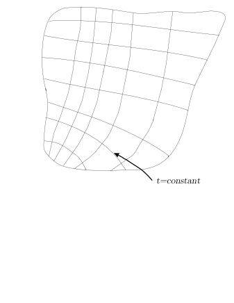
Figure 1: Basic canonical structure: space-time accepting two mutually orthogonal foliations.

If this is going to make sense, there must be a space-time metric tensor available at each tangent space such that scalar products can be taken. To be sure that such a space-time tensor does exist, we require that on ${\cal S}_{t}$, there must exist a family of scalar fields $N_{t}$ and a family of intrinsic spatial metrics ${\bf h}_{t}$. Moreover, there must exist a set of preferred coordinate systems where the time coordinate $x^{0}$ can be identified with the global time function $t$. We call such a coordinate system a global time coordinate system (GTCS). The coordinate motion of the FOs with respect to a GTCS defines a family ${\bf N}_{t}$ of spatial covector fields tangential to the FHSs. Now $N_{t}$, ${\bf N}_{t}$ and ${\bf h}_{t}$ uniquely determine a family of Lorentzian space-time metrics ${\bf g}_{t}$. This metric family may be thought of as constructed from measurements available to the FOs, if the functions $N_{t}$ are identified with the lapse functions describing the proper time elapsed as measured by the FOs, and if the covectors ${\bf N}_{t}$ are identified with the shift covector fields of the FOs in a GTCS. With the help of $N_{t}$ and ${\bf N}_{t}$, we may then construct the family of normal vector fields ${\bf n}_{t}$ being tangent vector fields to the world lines of the FOs and such that ${\bf h}_{t}({\bf n}_{t},{\cdot})=0$. Thus, by construction, the foliation of $({\cal N},{\bf g}_{t})$ into the set of world lines of the FOs is orthogonal to the foliation of $({\cal N},{\bf g}_{t})$ into the set of FHSs, as asserted. To illustrate this, we may write

$${\bf g}_{t}=-{\bf g}_{t}({\bf n}_{t},{\cdot}){\otimes}{\bf g}_{t}({\bf n}_{t},{\cdot})+{\bf h}_{t}.$$ (1)

Note that there is no reason to believe that any affine connection compatible with the above construction must be metric. Thus the point is to illustrate that it may be possible to create a geometrical structure where a space-time metric tensor is available at every event, but where the affine geometry does not necessarily follow exclusively from a space-time metric. The reason for this is that the existence of the global time function $t$ may be crucial when determining the affine connection; this possibility would not exist if the space-time geometry were required to be metric.

3 Connection and curvature

The existence of a Lorentzian space-time metric ${\bf g}{\in}{\bf g}_{t}$ for each FHS ${\cal S}{\in}{\cal S}_{t}$ implies that each FHS can be viewed as a spatial submanifold of a metric space-time manifold $({\cal M},{\bf g}_{t})$ for constant $t$ (at least locally). We now perform a mathematical trick inasmuch as whenever we take this viewpoint, we may define a global time coordinate $x^{0}$ on $({\cal M},{\bf g}_{t})$ such that $x^{0}=ct$ on each FHS; any coordinate system where this relationship holds is by definition a GTCS. We may then regard $x^{0}$ and $t$ as representing separate time dimensions such that $t=$constant on $({\cal M},{\bf g}_{t})$. It is thus possible to view $\cal N$ as a 4-dimensional submanifold of ${\cal M}{\times}{\bf R}$. The point of this, is that on the FHSs, we may take scalar products of fields defined on space-time in $({\cal M},{\bf g}_{t})$, whereas time derivatives of such fields depend on $t$ as well as on $x^{0}$ in $({\cal N},{\bf g}_{t})$. Thus the existence of extra time derivatives with respect to $t$ of ${\bf g}_{t}$, means that we can find an affine connection that is not fully determined by any single ${\bf g}{\in}{\bf g}_{t}$. See figure 2 for visualization of quasi-metric space-time geometry.

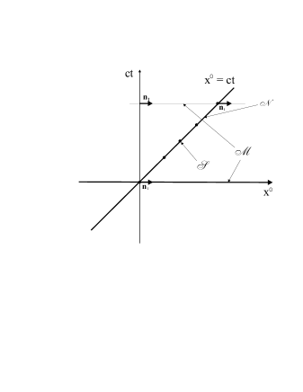
Figure 2: The geometrical structure of quasi-metric space-time, visualized.

Since each ${\bf g}{\in}{\bf g}_{t}$ is defined on a spatial submanifold only, there is in general no way to extend it to all of $\cal N$. However, the Levi-Civita connection corresponding to each ${\bf g}{\in}{\bf g}_{t}$ can be calculated on each FHS by holding $t$ constant. But this family of metric connections does not fully determine the connection compatible with the family ${\bf g}_{t}$. To find the full connection compatible with the family ${\bf g}_{t}$, it is convenient to view ${\bf g}_{t}$ as a single 5-dimensional degenerate metric on ${\cal M}{\times}{\bf R}$. One may then construct a linear, symmetric and torsion-free connection    on ${\cal M}{\times}{\bf R}$ by requiring that this connection is compatible with the non-degenerate part of the metric family ${\bf g}_{t}$, in addition to the condition that ${\,}{\begin{picture}(2.0,0.0)(-1.0,-1.4)\put(0.0,0.0){\makebox(0.0,0.0)[]{$\nabla$}} \put(0.0,2.4){\makebox(0.0,0.0)[]{\mbox{\tiny$\star$}}} \end{picture}}_{\frac{\partial}{{\partial}t}}{\bf n}_{t}$ vanishes. For obvious reasons, this connection is called “degenerate”, and it should come as no surprise that it is non-metric. One may then restrict the degenerate connection to $\cal N$ by just considering the submanifold $x^{0}=ct$ in a GTCS. For the exact form of the connection coefficients determining   , see, e.g., [2].

At this point, a natural question would be if there are physical phenomena which are naturally modelled by the non-metric part of quasi-metric geometry. And as we shall see in the main part of this thesis this is indeed the case.

4 Two simple examples

We finish this mathematical introduction by giving two simple examples. The first example illustrates how a family of space-time metrics can be represented by a family of line elements, whereas the second example illustrates how affinely parametrized curves are represented.

Example 1
A family of Minkowski metrics can be represented by the family of line elements

$$ds_{t}^{2}=-(dx^{0})^{2}+{\Xi}^{2}(t){\Big{(}}dx^{2}+dy^{2}+dz^{2}{\Big{)}},$$ (2)

where ${\Xi}(t)$ is a scale factor, $x^{0}=ct$ and $x,y,z$ are ordinary Cartesian coordinates. Note that the $t$-direction is treated as degenerate. It is easy to show that the free-fall curves obtained from the equations of motion (derived in chapter 1, section 5 of this thesis) and applied to equation (2), are different than their counterparts obtained by setting $dx^{0}=cdt$ in equation (2) and using the geodesic equation compatible with the resulting single metric.

Example 2
Let ${\{}t(\lambda),x^{\alpha}(\lambda){\}}$ represent an affinely parameterized curve, where $x^{\alpha}$ are space-time coordinates in a GTCS. Then the tangent vector field ${\frac{\partial}{{\partial}{\lambda}}}$ along the curve may be represented by the expression

$${\frac{\partial}{{\partial}{\lambda}}}={\frac{dt}{d{\lambda}}}{\frac{\partial}{{\partial}t}}+{\frac{dx^{\mu}}{d{\lambda}}}{\frac{\partial}{{\partial}x^{\mu}}}.$$ (3)

Now the length of ${\frac{\partial}{{\partial}{\lambda}}}$ may be calculated along the curve, e.g., for a timelike curve, ${\bf g}_{t}({\frac{\partial}{{\partial}{\lambda}}},{\frac{\partial}{{\partial}{\lambda}}})<0$ along the curve. On the other hand, the degenerate connection taken along ${\frac{\partial}{{\partial}{\lambda}}}$ is

$${\begin{picture}(2.0,0.0)(-1.0,-1.4)\put(0.0,0.0){\makebox(0.0,0.0)[]{$\nabla$}} \put(0.0,2.4){\makebox(0.0,0.0)[]{\mbox{\tiny$\star$}}} \end{picture}}_{{\frac{\partial}{{\partial}{\lambda}}}}={\frac{dt}{d{\lambda}}}{\begin{picture}(2.0,0.0)(-1.0,-1.4)\put(0.0,0.0){\makebox(0.0,0.0)[]{$\nabla$}} \put(0.0,2.4){\makebox(0.0,0.0)[]{\mbox{\tiny$\star$}}} \end{picture}}_{{\frac{\partial}{{\partial}t}}}+{\frac{dx^{\mu}}{d{\lambda}}}{\begin{picture}(2.0,0.0)(-1.0,-1.4)\put(0.0,0.0){\makebox(0.0,0.0)[]{$\nabla$}} \put(0.0,2.4){\makebox(0.0,0.0)[]{\mbox{\tiny$\star$}}} \end{picture}}_{{\frac{\partial}{{\partial}x^{\mu}}}}.$$ (4)

Thus we have illustrated that the degenerate part of ${\frac{\partial}{{\partial}{\lambda}}}$ does not contribute to its length (since ${\bf g}_{t}({\frac{\partial}{{\partial}t},{\cdot}}){\equiv}0$). However, as can be seen from equation (4), the degenerate part of ${\frac{\partial}{{\partial}{\lambda}}}$ does influence parallel-transport of space-time objects.

Hopefully, anyone who has understood the basic mathematical concepts underlying the quasi-metric framework, will not be so easily distracted by mathematical hurdles and will be in a better position to follow the derivation of the main results presented in this thesis. Accordingly, having read this mathematical introduction, the reader should now be ready for the main parts of the thesis.
References
[1] C.W. Misner, K.S. Thorne, J.A. Wheeler, Gravitation, W.H. Freeman ${\&}$ Co. (1973).
[2] D. Østvang, chapter 1, section 2 of this thesis (2001).

Chapter One:
 
A Non-Metric Approach to
Space, Time and Gravitation

A Non-Metric Approach to Space, Time and Gravitation

by

Dag Østvang

Institutt for fysikk, Norges teknisk-naturvitenskapelige universitet, NTNU
N-7491 Trondheim, Norway

1         Introduction

A proper description of nature’s fundamental forces involves their formulation as dynamical laws subject to appropriate initial conditions. This defines the initial-value problem for whatever dynamical system one wishes to study.

The initial-value problem for gravitation generally involves what one may loosely call “evolution of space with time”. More precisely, given a one-parameter family of 3-dimensional manifolds ${\cal S}_{t}$, each of which is identified as “space” at “time” $t$ (such that $t=$constant on each ${\cal S}{\in}{\cal S}_{t}$), the family defines an evolution of the 3-manifolds ${\cal S}_{t}$ with $t$. However, every conceivable theory of gravity includes an overlying 4-dimensional geometrical structure called “space-time” with which the given family must be compatible. Thus it is not possible to analyse a given family ${\cal S}_{t}$ in isolation; the evolution with $t$ of fields that determine the relationship between the family and the overlying space-time must be analysed simultaneously. When this is done one recovers the space-time geometry.

Naturally, the structure of any space-time framework should be more general than any particular theory of gravity formulated within that framework. This implies that in general, there should exist geometrical relations between the space-time framework and any given family ${\cal S}_{t}$ that do not depend on the detailed form of the dynamical laws one uses. A particular set of such relations is called kinematical relations (see, e.g., [1]). The kinematical relations of different space-time frameworks are recognized by their sharing of a common feature; that they are not sufficient by themselves to determine solutions of the initial-value problem. That is, in addition to the initial conditions, one must supply extra fields coming from the dynamics at each step of the evolution of ${\cal S}_{t}$ if one wants to recover the space-time geometry. Thus the kinematical relations explicitly exhibit the dependence on the existence of some coupling between geometry and matter fields, even if the detailed nature of the coupling is not specified. This is what one should expect, since any relations defined as kinematical always should give room for appropriate dynamics.

As a first example, we take the case of the stratified non-relativistic space-time framework of Newton-Cartan [4]. Here, there exists a unique family ${\cal S}_{t}$ consisting of Euclidean spaces (and left intact by Galilean transformations), where $t$ is Newton’s absolute time. The overlying geometrical structure belonging to this space-time is the space-time covariant derivative ${\nabla}$ represented by the only non-zero connection coefficients ${\Gamma}^{i}_{tt}{\equiv}{\Phi},_{i}$ (using a Cartesian coordinate system ${\{}x^{i}{\}}$). Here, ${\Phi}(t,x^{i})$ is a potential function and the comma denotes a partial derivative. The equation of motion for inertial test particles is the geodesic equation

$${\frac{d^{2}x^{i}}{dt^{2}}}+{\Gamma}^{i}_{tt}=0,$$ (1)

so to calculate the world lines of such test particles one must know ${\Gamma}^{i}_{tt}$ for every member of the family ${\cal S}_{t}$. Now we notice that there is a general relationship between the only non-zero components of the Riemann tensor and the potential function given by [4]

$$R_{itjt}={\frac{{\partial}^{2}}{{\partial}x^{i}{\partial}x^{j}}}{\Phi}={\frac{\partial}{{\partial}x^{i}}}{\Gamma}^{j}_{tt}.$$ (2)

That this relation is kinematical we see from the fact that, to determine the ${\Gamma}^{i}_{tt}$ for all times and thus all information relevant for the motion of inertial test particles, one must explicitly supply the tensor $R_{itjt}$ for each time step. Furthermore, equation (2) is valid regardless of the detailed coupling between $R_{itjt}$ and matter fields.

As a second example, we take the more realistic case of a metric relativistic space-time. In this case, the choice of family ${\cal S}_{t}$ is not unique, so the kinematical relations should be valid for any such choice. Furthermore, the overlying geometrical structure belonging to space-time is the space-time metric field, and this field induces relations between different choices of ${\cal S}_{t}$. Analogous to the first example, the kinematical relations are given by (using a general spatial coordinate system and applying Einstein’s summation convention)

$$R_{i{\perp}j{\perp}}=N^{-1}{\cal L}_{N{\bf n}}K_{ij}+{K_{i}}^{k}K_{kj}+c^{-2}a_{i{\mid}j}+c^{-4}a_{i}a_{j},$$ (3)

see, e.g., [1] for a derivation. Here, a is the 4-acceleration field of observers moving orthogonally to each ${\cal S}{\in}{\cal S}_{t}$, $N$ is their associated lapse function field and ‘$\perp$’ denotes projection onto the normal direction of ${\cal S}_{t}$. Furthermore, ${\cal L}_{\bf n}$ denotes the projected Lie derivative in the normal direction and ‘${\mid}$’ denotes a spatial covariant derivative intrinsic to each ${\cal S}{\in}{\cal S}_{t}$. The extrinsic curvature tensor K describes the curvature of each ${\cal S}{\in}{\cal S}_{t}$ relative to the overlying space-time curvature. There exists a well-known relationship between K and the evolution in the normal direction of the intrinsic geometry of each ${\cal S}{\in}{\cal S}_{t}$, namely (see, e.g., [1, 4])

$$K_{ij}=-{\frac{1}{2}}{\pounds}_{\bf n}h_{ij},$$ (4)

where £_n denotes a Lie derivative in the normal direction and ${\bf h}$ denotes the intrinsic metric of each ${\cal S}{\in}{\cal S}_{t}$. Another, geometrically equivalent expression of the kinematical relations (3), is found (see, e.g., [1]) by projecting the Einstein space-time tensor field ${\bf G}$ with respect to the spatial hypersurfaces ${\cal S}_{t}$. The projection of each space-time index may be a normal projection or a tangential projection, so for ${\bf G}$ we have 3 different projections since ${\bf G}$ is a symmetric tensor. The result is ($K{\equiv}{K^{k}}_{k}$)

$$G_{{\perp}{\perp}} = {\frac{1}{2}}(P+K^{2}-K_{ks}K^{ks}),{}$$

$$G_{{\perp}j} = (K^{k}_{j}-K{\delta}^{k}_{j})_{{\mid}k},{}$$

$$G_{ij} = -N^{-1}{\cal L}_{N{\bf n}}(K_{ij}-Kh_{ij})-2{K_{i}}^{k}K_{kj}+3KK_{ij}-{\frac{1}{2}}(K_{ks}K^{ks}+K^{2})h_{ij}{}$$ (5)

$$- c^{-2}(a_{i{\mid}j}-{a^{k}}_{{\mid}k}h_{ij})-c^{-4}(a_{i}a_{j}-a^{k}a_{k}h_{ij})+H_{ij},$$

where ${\bf H}$ and $P$ are, respectively, the Einstein tensor and the Ricci scalar intrinsic to the hypersurfaces. Equation (4) in combination with equation (3) (or equivalently, the totally spatial projection $G_{ij}$ shown in equation (5), the other projections representing constraints on initial data), may be recognized as kinematical equations. This follows from the fact that, in addition to initial values of $h_{ij}$ and $K_{ij}$ at an initial hypersurface, one needs to specify the tensor field $G_{ij}$ or equivalently, the tensor field $R_{i{\perp}j{\perp}}$, at each step of the evolution of ${\cal S}_{t}$ if one wishes to recover the space-time metric field and thus all information about the geometry of space-time as predicted at subsequent hypersurfaces. Note that this does not depend on Einstein’s equations being valid (see, e.g., [1] for a further discussion).

In light of the two above examples, we may call the evolution represented by a family ${\cal S}_{t}$ a kinematical evolution (KE) if it depends on the supplement of extra fields coming from an overlying geometrical structure at each step of the evolution. The question now is if this type of evolution exhausts all possibilities. The reason for this concern is, that one may possibly imagine a type of evolution of spatial hypersurfaces that does not depend on the supplement of extra fields at each step of the evolution. Rather, an evolution of such type should be given explicitly as an “absolute” property of space-time itself. It would be natural to call such a kind of evolution non-kinematical (NKE). Since, by construction, the NKE does not give room for dynamics, any geometrical framework having the capacity to accommodate both KE and NKE of a family ${\cal S}_{t}$ must be different from the standard metric framework.

As illustrated by the above examples, we see from equations (2) and (3) that the extra fields one must supply at each time step to get the KE working, take the form of curvature tensors. On the other hand, the NKE should be given explicitly and be obtainable as an intrinsic property of each member ${\cal S}$ of a unique family ${\cal S}_{t}$. Since we want our alternative space-time framework to be relativistic, $t$ must represent a “preferred” time coordinate and any member of the unique family ${\cal S}_{t}$ must represent a “preferred” notion of space. Observers moving normally to any ${\cal S}{\in}{\cal S}_{t}$ get the status of preferred observers. However, the existence of the unique family ${\cal S}_{t}$ does not imply that there exists a preferred coordinate frame in the sense that the outcomes of local experiments depend on the velocity with respect to it [2]. On the other hand, it will exist a class of “preferred” coordinate systems especially well adapted to the geometry of space-time. One may expect that equations take special forms in any such a coordinate system.

Now to the questions; are there physical phenomena which may be suspected to have something to do with the NKE and if so, do we get any hint of which form it should take? The fact that our Universe seems to be compatible with a preferred time coordinate at large scales, makes us turn to cosmology in an attempt to answer these questions. With the possibility of a rather dramatic reinterpretation of the Hubble law in mind, we guess that the NKE should take the form of a local increase in scale with time as measured by the above defined preferred observers. Moreover, this increase in scale should be described via a scale factor given explicitly as a function of $t$ and being part of the intrinsic geometry of each member ${\cal S}$ of the preferred family ${\cal S}_{t}$. That is, we guess that the Hubble law has nothing to do with kinematics; rather the Hubble law should be the basic empirical consequence of the (global) NKE.

The above guess represents the key to finding a new framework of space and time which incorporates both KE and NKE in a natural way. We call this new framework “quasi-metric” since it is not based on pseudo-Riemannian geometry and yet the new framework is compatible with important physical principles previously thought to hold for metric theory only. In this thesis, we explore some of the possibilities of the quasi-metric framework; among other things we derive a new theory of gravity. The thesis is organized as follows: in chapter 1 we define the quasi-metric framework and list the important results without going through all the gory details, while chapters 2, 3, 4 and 5 are self-contained articles containing the detailed calculations underlying the results listed in chapter 1.

2         An alternative framework of space and time

Our first problem is to arrive at a general framework describing space and time in a way compatible with the existence of both KE and NKE of ${\cal S}_{t}$, as discussed in the introduction. Since at least parts of the KE of any member ${\cal S}$ of the preferred family ${\cal S}_{t}$ should be described by a Lorentzian space-time metric ${\bf g}$, we may assume that the KE represented by ${\bf g}$ is discernible at each time step. That is, at least in a (infinitesimally) small time interval centred at the hypersurface $t=$constant, it should be possible to evolve this hypersurface purely kinematically in the hypersurface-orthogonal direction with the help of the 4-metric ${\bf g}$ without explicitly taking the NKE into account. But since this should be valid for every ${\cal S}{\in}{\cal S}_{t}$, to be compatible with the existence of any NKE, different ${\cal S}{\in}{\cal S}_{t}$ should be associated with different metrics ${\bf g}{\in}{\bf g}_{t}$. Thus the preferred family ${\cal S}_{t}$ of 3-dimensional spatial manifolds should define a one-parameter family of 4-dimensional Lorentzian metrics ${\bf g}_{t}$, the domain of validity of each being exactly the hypersurface $t=$constant, but such that one may extrapolate each metric at least in a (infinitesimally) small interval centred at this hypersurface.

We may think of the parameter $t$ as representing an extra time dimension, since fixing $t$ is equivalent to fixing a space-time metric ${\bf g}{\in}{\bf g}_{t}$ on (at least part of) a space-time 4-manifold. This indicates that the mathematically precise definition of the quasi-metric framework should involve a 5-dimensional product manifold ${\cal M}{\times}{\bf R}$ where ${\cal M}$ is a Lorentzian space-time manifold and ${\bf R}$ is the real line. We may then interpret $t$ as a global coordinate on ${\bf R}$ and the preferred family ${\cal S}_{t}$ as representing a foliation into spatial 3-manifolds of a 4-dimensional submanifold ${\cal N}$ of ${\cal M}{\times}{\bf R}$. Thus ${\cal N}$ is, by definition, a 4-dimensional space-time manifold equipped with a one-parameter family of Lorentzian metrics ${\bf g}_{t}$ in terms of the global time function $t$. This is the mathematical definition of the quasi-metric space-time framework we want to use as the basis for constructing a new relativistic theory of gravity.

Henceforth, we refer to the members of ${\cal S}_{t}$ as the fundamental hypersurfaces (FHSs). Observers always moving orthogonally to the FHSs are called fundamental observers (FOs). Note that the FOs are in general non-inertial. When doing calculations, it is often necessary to define useful coordinate systems. A particular class of coordinate systems especially well adapted to the existence of the FHSs, is the set of global time coordinate systems (GTCSs). A coordinate system ${\{}x^{\mu}{\}}$ is a GTCS if and only if the relationship in $\cal N$ between the time coordinate $x^{0}$ and the global time function $t$ is explicitly given by the equation $x^{0}=ct$. Since the local hypersurface-orthogonal direction in $\cal M$ is, by definition, physically equivalent to the direction along the world line of the local FO in $\cal N$, the one-parameter family of metrics is most conveniently expressed in a GTCS. That is, in a GTCS the spatial line elements of the FHSs evolve along the world lines of the FOs in $\cal N$; there is no need to worry about the explicit evolution of the spatial geometry along alternative world lines. Note that there exist infinitely many GTCSs due to the particular structure of quasi-metric space-time, but that in general, it is not possible to find one which with respect to the FOs are at rest. However, in particular cases, further simplification is possible if we can find a comoving coordinate system. A comoving coordinate system is by definition a coordinate system where the spatial coordinates are constants along the world lines of the FOs. A comoving coordinate system which is also a GTCS we conventionally call a hypersurface-orthogonal coordinate system (HOCS). Expressed in a HOCS, the 3-vector piece $g_{(t)0i}$ of ${\bf g}_{t}$ vanishes. But in general, it is not possible to find a HOCS; that is possible for particular cases only.

The condition that the global time function should exist everywhere, implies that in ${\cal M}$, each FHS must be a Cauchy hypersurface for every allowable metric ${\bf g}{\in}{\bf g}_{t}$. Furthermore, each FHS must be a member of a family of hypersurfaces foliating ${\cal M}$ equipped with any allowable metric ${\bf g}{\in}{\bf g}_{t}$ when this metric is extrapolated off the FHS. Note that the hypothetical observers moving orthogonal to this family of hypersurfaces may be thought of as FOs with the explicit NKE “turned off” and that the normal curves of these hypersurfaces are in general not geodesics of ${\bf g}{\in}{\bf g}_{t}$.

Actually, it may not be possible to eliminate all the effects of the NKE just by holding $t$ constant. The reason for this, is the possibility that some of the NKE, which we will call the local NKE, is not “realized” explicitly. That is, the FOs may move in a way such that the “expansion” representing the local NKE is exactly cancelled out. In other words, the FOs may be thought of as “falling” with a 3-velocity $-{\bf v}_{t}$ and simultaneously expanding with a 3-velocity ${\bf v}_{t}$ due to the local NKE, the net result being “stationariness”. But this type of stationariness is not equivalent to being stationary with no NKE; for example one typically gets time dilation factors associated with the extra “motion”. Now the effects of the local NKE should be compensated for in the “physical” metric family ${\bf g}_{t}$. On the other hand, said effects should in general be present implicitly and uncompensated for in solutions of field equations. This means that ${\bf g}_{t}$ cannot represent a solution of field equations. To overcome this problem, we introduce a second metric family ${\bf{\bar{g}}}_{t}$ on a corresponding product manifold ${\overline{\cal M}}{\times}{\bf R}$ and consider a 4-dimensional submanifold ${\overline{\cal N}}$ just as for the family ${\bf g}_{t}$. The crucial difference is that the family ${\bf{\bar{g}}}_{t}$ by definition represents a solution of appropriate field equations. Thus when we construct such field equations, we will study the general properties of ${\bf{\bar{g}}}_{t}$ rather than those of ${\bf g}_{t}$. Any local non-kinematical features, disguised as kinematical features belonging to the metric structure of each member of the family ${\bf{\bar{g}}}_{t}$, must then be compensated for via a transformation ${\bf{\bar{g}}}_{t}{\rightarrow}{\bf g}_{t}$ involving the vector field family ${\bf v}_{t}$.

The family of hypersurfaces foliating ${\cal M}$ (or ${\overline{\cal M}}$) equipped with any allowable metric ${\bf g}{\in}{\bf g}_{t}$ (or ${\bf{\bar{g}}}{\in}{\bf{\bar{g}}}_{t}$) defines a one-parameter family of 3-manifolds in terms of a suitably defined time coordinate function $x^{0}$. A sufficient condition to ensure the existence and uniqueness of the global time coordinate function $x^{0}$ on ${\cal M}$ (or ${\overline{\cal M}}$) such that the gradient field of this coordinate is everywhere timelike, is to demand that each FHS is compact (without boundaries) [3]. Assuming simple topology, this should imply the existence of some prior 3-geometry of the FHSs; interpreted as a cosmological “background” 3-geometry, and chosen to be the geometry of the 3-sphere ${\bf S}^{3}$. It is expected that this 3-geometry will show up via specific terms in the field equations.

We now write down a general expression for the metric family ${\bf{\bar{g}}}_{t}$, where the explicit dependence on $t$ represents the global NKE of the FHSs (and the other pieces of ${\bf{\bar{g}}}_{t}$). That is, expressed in a suitable GTCS (using Einstein’s summation convention), the most general form allowed for the family ${\bf{\bar{g}}}_{t}$ is represented by the family of line elements valid on the FHSs (this may be taken as a definition)

$${\overline{ds}}_{t}^{2}={\bar{N}}_{t}^{2}{\Big{\{}}[{\bar{N}}_{(t)}^{k}{\bar{N}}_{(t)}^{s}{\tilde{h}}_{(t)ks}-1](dx^{0})^{2}+2{\frac{t}{t_{0}}}{\bar{N}}_{(t)}^{k}{\tilde{h}}_{(t)ks}dx^{s}dx^{0}+{\frac{t^{2}}{t_{0}^{2}}}{\tilde{h}}_{(t)ks}dx^{k}dx^{s}{\Big{\}}}.$$ (6)

Here, $t_{0}$ is some arbitrary reference epoch (usually chosen to be the present epoch) setting the scale of the spatial coordinates, ${\bar{N}}_{t}$ is the family of lapse functions of the FOs and ${\frac{t_{0}}{t}}{\bar{N}}^{k}_{(t)}$ are the components of the shift vector family of the FOs in ${\overline{\cal N}}$. Also, ${\bf{\bar{h}}}_{t}$, with components ${\bar{h}}_{(t)ks}{\equiv}{\frac{t^{2}}{t_{0}^{2}}}{\bar{N}}_{t}^{2}{\tilde{h}}_{(t)ks}$, is the spatial metric family intrinsic to the FHSs. Moreover, as a counterpart to equation (6), a general form for the family ${\bf g}_{t}$ is given by the family of line elements (using a GTCS)

$${ds}_{t}^{2}=[N_{(t)}^{k}N_{(t)}^{s}{\hat{h}}_{(t)ks}-N^{2}](dx^{0})^{2}+2{\frac{t}{t_{0}}}N_{(t)}^{k}{\hat{h}}_{(t)ks}dx^{s}dx^{0}+{\frac{t^{2}}{t_{0}^{2}}}{\hat{h}}_{(t)ks}dx^{k}dx^{s},$$ (7)

where the symbols have similar meanings to their (barred) counterparts in equation (6) (the counterpart to ${\bar{h}}_{(t)ks}$ is $h_{(t)ks}{\equiv}{\frac{t^{2}}{t_{0}^{2}}}{\hat{h}}_{(t)ks}$). Note that the propagation of sources (and test particles) is calculated by using the equations of motion in ${\cal N}$ (see equation (15) below). Besides, since the proper time as measured along a world line of a FO should not directly depend on the cosmic expansion, the lapse function $N$ should not depend explicitly on $t$. Therefore, any potential $t$-dependence of $N$ must be eliminated by substituting $t$ with $x^{0}/c$ (using a GTCS) whenever it occurs before using the equations of motion. In the same way, any extra $t$-dependence of ${\bf g}_{t}$ coming from the transformation ${\bf{\bar{g}}}_{t}{\rightarrow}{\bf g}_{t}$ must be eliminated. Consequently, any $t$-dependence of ${\hat{h}}_{(t)ks}$ will stem from that of ${\tilde{h}}_{(t)ks}$.

Next, an obvious question is which sort of affine structure is induced on ${\cal N}$ by the family of metrics ${\bf g}_{t}$ (and analogously which affine structure is induced on ${\overline{\cal N}}$ by ${\bf{\bar{g}}}_{t}$). To answer this question, it is convenient to perceive ${\bf g}_{t}$ as a single degenerate 5-dimensional metric on ${\cal M}{\times}{\bf R}$ and construct a torsion-free connection      almost compatible with ${\bf g}_{t}$ (     yields non-metricity for the degenerate part of ${\bf g}_{t}$). But in addition to almost metric-compatibility, i.e., ${\,}{\begin{picture}(2.0,0.0)(-1.0,-1.4)\put(0.0,0.0){\makebox(0.0,0.0)[]{$\nabla$}} \put(0.0,2.4){\makebox(0.0,0.0)[]{\mbox{\tiny$\star$}}} \end{picture}}_{\frac{\partial}{{\partial}t}}{\bf g}_{t}=0$, we should also require that the unit normal vector field family of the FHSs does not change when it is parallel-transported in the $t$-direction. That is, we should require that ${\,}{\begin{picture}(2.0,0.0)(-1.0,-1.4)\put(0.0,0.0){\makebox(0.0,0.0)[]{$\nabla$}} \put(0.0,2.4){\makebox(0.0,0.0)[]{\mbox{\tiny$\star$}}} \end{picture}}_{\frac{\partial}{{\partial}t}}{\bf n}_{t}$ vanishes. When a connection satisfying these requirements is found, we can restrict it to ${\cal N}$ and we have the wanted affine structure.

In order to construct      on ${\cal M}{\times}{\bf R}$, the metric-preserving condition

$${\frac{\partial}{{\partial}t}}{\bf g}_{t}({\bf y}_{t},{\bf z}_{t})={\bf g}_{t}({\,}{\,}{\begin{picture}(2.0,0.0)(-1.0,-1.4)\put(0.0,0.0){\makebox(0.0,0.0)[]{$\nabla$}} \put(0.0,2.4){\makebox(0.0,0.0)[]{\mbox{\tiny$\star$}}} \end{picture}}_{\frac{\partial}{{\partial}t}}{\bf y}_{t},{\bf z}_{t})+{\bf g}_{t}({\bf y}_{t},{\begin{picture}(2.0,0.0)(-1.0,-1.4)\put(0.0,0.0){\makebox(0.0,0.0)[]{$\nabla$}} \put(0.0,2.4){\makebox(0.0,0.0)[]{\mbox{\tiny$\star$}}} \end{picture}}_{\frac{\partial}{{\partial}t}}{\bf z}_{t}),$$ (8)

involving arbitrary families of vector fields ${\bf y}_{t}$ and ${\bf z}_{t}$ in ${\cal M}$, may be used to find a candidate connection where the connection coefficients are determined from ${\bf g}_{t}$ alone. It turns out that such a candidate connection is unique and that its difference from the usual Levi-Civita connection is determined from the only non-zero connection coefficients containing $t$. These are given by ${\begin{picture}(2.0,0.0)(-1.0,-1.4)\put(0.0,0.0){\makebox(0.0,0.0)[]{$\Gamma$}} \put(0.0,2.4){\makebox(0.0,0.0)[]{\mbox{\tiny$\star$}}} \end{picture}}^{{\,}{\alpha}}_{{\mu}t}$ and are equal to ${\frac{1}{2}}g_{(t)}^{{\alpha}{\sigma}}{\frac{\partial}{{\partial}t}}g_{(t){\mu}{\sigma}}$. (Here we have introduced the coordinate notation $g_{(t){\mu}{\sigma}}$ for the family ${\bf g}_{t}$.) But this candidate connection does in general not satisfy the criterion ${\,}{\begin{picture}(2.0,0.0)(-1.0,-1.4)\put(0.0,0.0){\makebox(0.0,0.0)[]{$\nabla$}} \put(0.0,2.4){\makebox(0.0,0.0)[]{\mbox{\tiny$\star$}}} \end{picture}}_{\frac{\partial}{{\partial}t}}{\bf n}_{t}=0$. However, the part of it involving ${\bf h}_{t}$ does, provided that (where a comma denotes taking a partial derivative)

$${\frac{\partial}{{\partial}t}}{\Big{[}}N_{(t)}^{k}N_{(t)}^{s}{\hat{h}}_{(t)ks}{\Big{]}}=0,\qquad{\Rightarrow}\qquad N_{(t),t}^{s}=-{\frac{1}{2}}N_{(t)}^{k}{\hat{h}}_{(t)}^{is}{\hat{h}}_{(t)ik,t}.$$ (9)

We may thus choose the connection coefficients equal to the hypersurface-intrinsic part ${\frac{1}{2}}h_{(t)}^{ik}{\frac{\partial}{{\partial}t}}h_{(t)jk}$ of the above-mentioned candidate connection coefficients. In addition, the shift vector field family is required to fulfil equation (9). We then have the unique non-zero connection coefficients

$${\begin{picture}(2.0,0.0)(-1.0,-1.4)\put(0.0,0.0){\makebox(0.0,0.0)[]{$\Gamma$}} \put(0.0,2.4){\makebox(0.0,0.0)[]{\mbox{\tiny$\star$}}} \end{picture}}_{tj}^{{\,}i}={\frac{1}{2}}h_{(t)}^{is}h_{(t)sj,t}={\frac{1}{t}}{\delta}^{i}_{j}+{\frac{1}{2}}{\hat{h}}_{(t)}^{is}{\hat{h}}_{(t)sj,t},{\qquad}{\begin{picture}(2.0,0.0)(-1.0,-1.4)\put(0.0,0.0){\makebox(0.0,0.0)[]{$\Gamma$}} \put(0.0,2.4){\makebox(0.0,0.0)[]{\mbox{\tiny$\star$}}} \end{picture}}^{{\,}{\alpha}}_{t{\mu}}{\equiv}{\ }{\begin{picture}(2.0,0.0)(-1.0,-1.4)\put(0.0,0.0){\makebox(0.0,0.0)[]{$\Gamma$}} \put(0.0,2.4){\makebox(0.0,0.0)[]{\mbox{\tiny$\star$}}} \end{picture}}^{{\,}{\alpha}}_{{\mu}t},$$ (10)

valid in a GTCS. The other connection coefficients not containing $t$-indices are found by requiring that they should be identical to those found from the family of Levi-Civita connections explicitly defined by the ${\bf g}_{t}$. It may be readily shown that equations (9) and (10), together with the explicit $t$-dependence of ${\bf g}_{t}$ shown in equation (7), yield

$${\begin{picture}(2.0,0.0)(-1.0,-1.4)\put(0.0,0.0){\makebox(0.0,0.0)[]{$\nabla$}} \put(0.0,2.4){\makebox(0.0,0.0)[]{\mbox{\tiny$\star$}}} \end{picture}}_{\frac{\partial}{{\partial}t}}{\bf g}_{t}=0,\qquad{\begin{picture}(2.0,0.0)(-1.0,-1.4)\put(0.0,0.0){\makebox(0.0,0.0)[]{$\nabla$}} \put(0.0,2.4){\makebox(0.0,0.0)[]{\mbox{\tiny$\star$}}} \end{picture}}_{\frac{\partial}{{\partial}t}}{\bf n}_{t}=0,\qquad{\begin{picture}(2.0,0.0)(-1.0,-1.4)\put(0.0,0.0){\makebox(0.0,0.0)[]{$\nabla$}} \put(0.0,2.4){\makebox(0.0,0.0)[]{\mbox{\tiny$\star$}}} \end{picture}}_{\frac{\partial}{{\partial}t}}{\bf h}_{t}=0,$$ (11)

thus the connection    has the desired properties. The restriction of      to $\cal N$ is trivial inasmuch as the same formulae are valid in $\cal N$ as in ${\cal M}{\times}{\bf R}$, the only difference being the restriction $x^{0}=ct$ in a GTCS.

Now we want to use the above defined affine structure on ${\cal N}$ to find equations of motion for test particles. Let ${\lambda}$ be an affine parameter along the world line of an arbitrary test particle. (In addition to the affine parameter $\lambda$, $t$ is also a (non-affine) parameter along any non-spacelike curve in $\cal N$.) If we define coordinate vector fields ${\frac{\partial}{{\partial}x^{\alpha}}}$, the coordinate representation of the tangent vector field ${\frac{\partial}{{\partial}{\lambda}}}$ along the curve is given by ${\frac{dt}{d{\lambda}}}{\frac{\partial}{{\partial}t}}+{\frac{dx^{\alpha}}{d{\lambda}}}{\frac{\partial}{{\partial}x^{\alpha}}}$. We then define the covariant derivative along the curve as

$${\begin{picture}(2.0,0.0)(-1.0,-1.4)\put(0.0,0.0){\makebox(0.0,0.0)[]{$\nabla$}} \put(0.0,2.4){\makebox(0.0,0.0)[]{\mbox{\tiny$\star$}}} \end{picture}}_{\frac{\partial}{{\partial}{\lambda}}}{\equiv}{\frac{dt}{d{\lambda}}}{\begin{picture}(2.0,0.0)(-1.0,-1.4)\put(0.0,0.0){\makebox(0.0,0.0)[]{$\nabla$}} \put(0.0,2.4){\makebox(0.0,0.0)[]{\mbox{\tiny$\star$}}} \end{picture}}_{\frac{\partial}{{\partial}t}}+{\frac{dx^{\alpha}}{d{\lambda}}}{\begin{picture}(2.0,0.0)(-1.0,-1.4)\put(0.0,0.0){\makebox(0.0,0.0)[]{$\nabla$}} \put(0.0,2.4){\makebox(0.0,0.0)[]{\mbox{\tiny$\star$}}} \end{picture}}_{\frac{\partial}{{\partial}x^{\alpha}}}.$$ (12)

A particularly important family of vector fields is the 4-velocity tangent vector field family ${\bf u}_{t}$ of a curve. That is, by definition we have

$${\bf u}_{t}{\equiv}u_{(t)}^{\alpha}{\frac{\partial}{{\partial}x^{\alpha}}}{\equiv}{\frac{dx^{\alpha}}{d{\tau}_{t}}}{\frac{\partial}{{\partial}x^{\alpha}}},$$ (13)

where ${\tau}_{t}$ is the proper time as measured along the curve.

The equations of motion are found by calculating the covariant derivative of 4-velocity tangent vectors along themselves using the connection in $\cal N$. According to the above, this is equivalent to calculating ${\,}{\,}{\begin{picture}(2.0,0.0)(-1.0,-1.4)\put(0.0,0.0){\makebox(0.0,0.0)[]{$\nabla$}} \put(0.0,2.4){\makebox(0.0,0.0)[]{\mbox{\tiny$\star$}}} \end{picture}}{\,}{\,}{\bf u}_{t}$ along ${\frac{\partial}{{\partial}{\tau}_{t}}}$. Using the coordinate representation of ${\frac{\partial}{{\partial}{\tau}_{t}}}$ in an arbitrary coordinate system, we may thus define the vector field ${\stackrel{{\scriptstyle\star}}{{\bf a}}}$ by

$${\stackrel{{\scriptstyle\star}}{{\bf a}}}{\equiv}{\stackrel{{\scriptstyle\star}}{{\nabla}}}_{\frac{\partial}{{\partial}{\tau}_{t}}}{\bf u}_{t}={\Big{(}}{\frac{dt}{d{\tau}_{t}}}{\stackrel{{\scriptstyle\star}}{{\nabla}}}_{\frac{\partial}{{\partial}t}}+{\frac{dx^{\alpha}}{d{\tau}_{t}}}{\nabla}_{\frac{\partial}{{\partial}x^{\alpha}}}{\Big{)}}{\bf u}_{t}{\equiv}{\frac{dt}{d{\tau}_{t}}}{\stackrel{{\scriptstyle\star}}{{\nabla}}}_{\frac{\partial}{{\partial}t}}{\bf u}_{t}+{\bf a}_{t},$$ (14)

where ${\bf a}_{t}$ is the ordinary 4-acceleration family. We call the vector field ${\stackrel{{\scriptstyle\star}}{{\bf a}}}$ the “degenerate” 4-acceleration. It may be shown that ${\stackrel{{\scriptstyle\star}}{{\bf a}}}$ is orthogonal to ${\bf u}_{t}$.

The coordinate expression for ${\stackrel{{\scriptstyle\star}}{{\bf a}}}$ shows that this yields equations of motion, namely

$${\frac{d^{2}x^{\alpha}}{d{\lambda}^{2}}}+{\Big{(}}{\begin{picture}(2.0,0.0)(-1.0,-1.4)\put(0.0,0.0){\makebox(0.0,0.0)[]{$\Gamma$}} \put(0.0,2.4){\makebox(0.0,0.0)[]{\mbox{\tiny$\star$}}} \end{picture}}^{{\,}{\alpha}}_{t{\sigma}}{\frac{dt}{d{\lambda}}}+{\Gamma}^{\alpha}_{(t){\beta}{\sigma}}{\frac{dx^{\beta}}{d{\lambda}}}{\Big{)}}{\frac{dx^{\sigma}}{d{\lambda}}}={\Big{(}}{\frac{d{\tau}_{t}}{d{\lambda}}}{\Big{)}}^{2}{\stackrel{{\scriptstyle\star}}{{a}}}^{\alpha}.$$ (15)

To get these equations to work, the degenerate 4-acceleration must be specified independently for each time step; thus they are kinematical equations. But ${\stackrel{{\scriptstyle\star}}{{\bf a}}}$ cannot be chosen freely. That is, given an initial tangent vector of the world line of an arbitrary test particle, as we can see from equation (14), ${\stackrel{{\scriptstyle\star}}{{\bf a}}}$ is uniquely determined by ${\bf a}_{t}$ and ${\frac{dt}{d{\tau}_{t}}}{\stackrel{{\scriptstyle\star}}{{\nabla}}}_{\frac{\partial}{{\partial}t}}{\bf u}_{t}$. However, in a subsequent section we will see that ${\stackrel{{\scriptstyle\star}}{{\nabla}}}_{\frac{\partial}{{\partial}t}}{\bf u}_{t}$ vanishes so we in fact have ${\stackrel{{\scriptstyle\star}}{{\bf a}}}$=${\bf a}_{t}$.

Now ${\bf a}_{t}$ has the usual interpretation as an expression for the inertial forces experienced by the test particle. Moreover, the coordinate expression for ${\bf a}_{t}$ in ${\cal M}$ is given by

$${\frac{d^{2}x^{\alpha}}{d{\lambda}^{2}}}+{\Gamma}^{\alpha}_{(t){\sigma}{\rho}}{\frac{dx^{\rho}}{d{\lambda}}}{\frac{dx^{\sigma}}{d{\lambda}}}{\equiv}{\Big{(}}{\frac{d{\tau}_{t}}{d{\lambda}}}{\Big{)}}^{2}a^{\alpha}_{(t)}.$$ (16)

However, to find the curves of test particles, equation (15) will be solved rather than equation (16); the latter is insufficient for this task since it does not take into account the dependence of ${\bf u}_{t}$ on $t$, i.e., it holds only in $\cal M$.

3         The role of gravity

We are now able to set up the postulates which must be satisfied for every theory of gravity compatible with the quasi-metric framework. These are (postulates for the metric framework [5] are stated in parenthesis for comparison)

• Space-time is equipped with a metric family ${\bf g}_{t}$ as described in the previous section, (metric theory: space-time is equipped with one single Lorentzian metric),

• Inertial test particles follow curves for which ${\bf a}_{t}=0$ calculated from (15), (metric theory: the curves are geodesics calculated from (16)),

• In the local inertial frames of ${\bf g}_{t}$, the non-gravitational physics is as in special relativity. (Metric theory: in the local Lorentz frames of the metric, the non-gravitational physics is as in special relativity.)

The third postulate means that we may always find a local coordinate system such that the connection coefficients in equation (15) vanish. Later we will see that in fact ${\stackrel{{\scriptstyle\star}}{{\bf a}}}$=${\bf a}_{t}$, meaning that inertial test particles follow geodesics of   , see equations (50), (51) and the subsequent discussion for verification. Thus the local inertial frames of ${\bf g}_{t}$ can be identified with local Lorentz frames, just as in metric theory. This means that there can be no local consequences of curved space-time for the non-gravitational physics. But it is important to notice that this applies strictly locally. That is, at any finite scale the geodesics of    do not coincide with the geodesics of any single space-time metric as long as there is a dependence on $t$. This means that the non-gravitational physics at any finite scale may vary in a way incompatible with any metric geometry. Despite this, any allowable theory does possess local Lorentz invariance (LLI), and furthermore it follows that we do have local position invariance (LPI), but that deviations from metric theory should be detectable at any finite scale. (LPI is by definition that the outcome of any local non-gravitational test experiment is independent of where or when it is performed.)

The second postulate ensures that the WEP is valid (i.e., that the free-fall curves traced out by test particles are independent of the particles’ internal structure). The sum of LLI, LPI and the WEP is called the Einstein equivalence principle (EEP) [5] and it is satisfied by any metric theory of gravity. Note that the EEP was previously thought to hold for metric theories only. Nevertheless, despite the differences in mathematical structure, the EEP should also hold for the class of quasi-metric gravitational theories according to the arguments made above.

Now we want to construct a theory of gravity satisfying the above postulates. This particular theory should contain no extra independent gravitational fields other than ${\bf{\bar{g}}}_{t}$ and also no prior 4-geometry. Since the quasi-metric framework fulfils LLI and LPI, we might hope to construct a theory which also embodies the strong equivalence principle (SEP) (that the EEP is valid for self-gravitating bodies and local gravitational test experiments as well as for test particles). But as we shall see, the quasi-metric framework predicts scale variations in space-time between non-gravitational and gravitational systems, and this is not compatible with the SEP in its most stringent interpretation. So we cannot ask for more than that the gravitational weak equivalence principle (GWEP) is satisfied (that the WEP is valid for self-gravitating bodies as well as for test particles). However, if the GWEP is not violated, this is sufficient to eliminate the most serious effects resulting from the violation of the SEP.

One distinct feature of our framework is the existence of a unique set of FHSs. This means that we can split up the metrics ${\bf{\bar{g}}}_{t}$ into space and time in a preferred way; i.e., we have a preferred family of unit normal vector fields ${\bf{\bar{n}}}_{t}$. In addition we have the 3-metrics ${\bf{\bar{h}}}_{t}$ intrinsic to the FHSs. We may then define a family of 4-acceleration fields ${\bf{\bar{a}}}_{\cal F}$ by

$$c^{-2}{\bar{a}}_{\cal F}^{\mu}{\equiv}{\bar{n}}_{(t);{\nu}}^{\mu}{\bar{n}}_{(t)}^{\nu},$$ (17)

where ‘;’ denotes taking a covariant derivative obtained from the metric connection ${\bf{\bar{\nabla}}}$ compatible with any single metric ${\bf{\bar{g}}}{\in}{\bf{\bar{g}}}_{t}$.

It is useful to denote a scalar product of any space-time object with $-{\bf{\bar{n}}}_{t}$ by the symbol ‘${\bar{\perp}}$’; this operation defines a normal projection. Analogously, any projection into a FHS may be performed by taking scalar products with ${\bf{\bar{h}}}_{t}$. To avoid confusion about whether we are dealing with a space-time object or a space object intrinsic to the FHSs, we will label space objects with a “hat” if necessary. That is, a maximal number of projections of the space-time object ${\bf{\bar{A}}}_{t}$ with $-{\bf{\bar{n}}}_{t}$ or ${\bf{\bar{h}}}_{t}$ will result in various space objects ${\bf{\hat{\bar{A}}}}_{t}$ (which object will depend on the exact projections made).

Thus, by repeated projections with $-{\bf{\bar{n}}}_{t}$ or ${\bf{\bar{h}}}_{t}$, any space-time object eventually reduces to a space object. For example, the space-time vector field ${\bf{\bar{a}}}_{\cal F}$ has the normal projection ${\bar{a}}_{{\cal F}{\bar{\perp}}}{\equiv}-{\bar{a}}^{\alpha}_{\cal F}{\bar{n}}_{(t){\alpha}}$, and the components of the horizontal projection are just ${\bar{a}}_{{\cal F}}^{j}$. In particular, one may easily show that

$${\bar{a}}_{{\cal F}{\bar{\perp}}}=0,{\qquad}c^{-2}{\bar{a}}_{{\cal F}j}={\frac{\partial}{{\partial}x^{j}}}{\ln}{\bar{N}}_{t}.$$ (18)

Furthermore, we define another useful quantity

$$c^{-2}{\bar{x}}_{t}+c^{-1}{\bar{y}}_{t}{\equiv}-{\frac{{\bar{N}}_{t},_{\bar{\perp}}}{{\bar{N}}_{t}}}+{\frac{{\bar{N}}_{t},_{t}}{c{\bar{N}}_{t}^{2}}},$$ (19)

which describes how ${\bar{N}}_{t}$ changes in the direction normal to the FHSs. The reason why the left hand side of equation (19) consists of two terms, is that the first term represents the KE of ${\bar{N}}_{t}$ and the second term represents the NKE of ${\bar{N}}_{t}$. We also notice that the family of extrinsic curvature tensors ${\bf{\bar{K}}}_{t}$ corresponding to the metric family ${\bf{\bar{g}}}_{t}$ of the type given in equation (6) has the form (in a GTCS)

$${\bar{K}}_{(t)ij}={\Big{(}}{\frac{{\bar{N}}_{t},_{\bar{\perp}}}{{\bar{N}}_{t}}}-{\frac{t_{0}}{t}}c^{-2}{\bar{a}}_{{\cal F}k}{\frac{{\bar{N}}_{(t)}^{k}}{{\bar{N}}_{t}}}{\Big{)}}{\bar{h}}_{(t)ij}+{\frac{t}{2{\bar{N}}_{t}t_{0}}}({\bar{N}}_{(t)i{\mid}j}+{\bar{N}}_{(t)j{\mid}i})-{\frac{1}{2}}{\frac{t^{2}}{t_{0}^{2}}}{\bar{N}}_{t}{\frac{\partial}{{\partial}x^{0}}}{\tilde{h}}_{(t)ij}.$$ (20)

Now we want to postulate what the nature of gravity should be in our theory. To arrive at that, we notice that the lapse function ${\bar{N}}_{t}$ in equation (6) also plays the role of a spatial scale factor. This means that we may think of ${\bar{N}}_{t}^{2}$ as a conformal factor in equation (6). We may then interpret ${\bar{N}}_{t}$ as resulting from a position-dependent units transformation. This indicates that the scale factor ${\bar{F}}_{t}{\equiv}{\bar{N}}_{t}ct$ of the FHSs may be thought of as representing a difference in scale between atomic and gravitational systems. That is, ${\bar{F}}_{t}$ may be thought of as representing a gravitational scale measured in atomic units. An equivalent way of interpreting ${\bar{F}}_{t}$ is to postulate that fixed operationally defined “atomic” units are considered formally variable throughout space-time. Since the intercomparison of operationally defined units only has meaning locally for objects at rest with respect to each other, any non-local intercomparison is purely a matter of definition [7].

The variation in scale between gravitational and atomic systems means that gravitational quantities get an extra formal variation when measured in atomic units (and vice versa); in particular the dimensional constants of nature may depend on this formal variation. That is, the “constants” of nature may in principle depend on whether they are expressed in atomic or gravitational units. We notice that, when performing a units transformation, we are free to define as constants physical constants that cannot be related to each other by dimensionless numbers [6]. We exploit this fact by defining $c$ and Planck’s constant ${\hbar}$ not to be formally variable. This means that measured in atomic units, the variation of gravitational lengths and times are identical and inverse to that of gravitational energy (or mass).

The requirement that $c$ and ${\hbar}$ are not formally variable, yields no restrictions on any possible relationship between the variation of units and physical fields. On the other hand, we may combine the unit charge $e$ with ${\hbar}$ and $c$ to form the dimensionless number $e^{2}/{\hbar}c$. Thus by defining $e$ not to be formally variable (so that gravitational charge units will not be formally variable), we deny any possible direct connection between gravitation and electromagnetism.

Formally variable atomic units represent changes of scale between non-gravitational and gravitational systems, and such changes of scale should be described by the metric family ${\bf{\bar{g}}}_{t}$. Moreover, ${\bf{\bar{g}}}_{t}$ should be found from field equations. We now define the scalar field ${\Psi}_{t}$; by definition ${\Psi}_{t}$ tells how atomic time units vary in space-time. Any gravitational quantity is associated with ${\Psi}_{t}$ to some power describing how the quantity changes due to the formal variation in scale between gravitational and atomic systems. In particular, we find from dimensional analysis that the “bare” gravitational coupling parameter $G_{t}^{\rm B}$ formally has the dimension of time (or length) units squared. Since $G_{t}^{\rm B}$ is a gravitational quantity, measured in atomic units it will then vary as a factor ${\Psi}_{t}^{-2}$. Besides, since charge is not formally variable, $G_{t}^{\rm B}$ couples to charge squared (as can be seen, e.g., from the well-known Reissner-Nordström solution in General Relativity (GR)), or more generally, to the electromagnetic stress-energy tensor. On the other hand, for material sources, masses formally vary as ${\Psi}_{t}$, but this is not measurable in non-gravitational experiments. Now the “screened” gravitational coupling parameter $G_{t}^{\rm S}$ couples to mass, and measured for material sources, said formal variation of mass means that $G_{t}^{\rm S}$ effectively varies as ${\Psi}_{t}^{-1}$. Thus we must have two (in general different) gravitational coupling parameters, so we cannot have universal coupling between matter and gravitation since the coupling will depend on the nature of the gravitational source. This represents a radical departure from GR. Notice that $G_{t}^{\rm B}$ and $G_{t}^{\rm S}$ will have different time dependences so they are not likely to be approximately equal at the present epoch. But by varying the composition of the gravitational source in a series of controlled experiments, it should in principle be possible to measure both $G_{t}^{\rm B}$ and $G_{t}^{\rm S}$ directly at the present epoch.

Since $G_{t}^{\rm B}$ and $G_{t}^{\rm S}$ usually occur in combination with charge or mass, it is convenient to define $G_{t}^{\rm B}$ and $G_{t}^{\rm S}$ to take the constant values $G^{\rm B}$ and $G^{\rm S}$, respectively, as measured in (hypothetical) local gravitational experiments in an empty universe at epoch $t_{0}$. But then one must distinguish between active mass $m_{t}$ measured dynamically as a source of gravity and passive mass $m$ (i.e., passive gravitational mass or inertial mass). This means that we include the formal variations of $G_{t}^{\rm B}$ or $G_{t}^{\rm S}$ into $m_{t}$, turning any active mass $m_{t}$ into a scalar field. That is, unlike $c$, ${\hbar}$ and $e$, $m_{t}$ gets a formal variation when measured in atomic units. We then find that the formal variation of active mass goes as ${\Psi}_{t}^{-2}$ for the electromagnetic field and as ${\Psi}_{t}^{-1}$ for material particles. In practice, this means that the effective gravitational “constant” $G^{\rm eff}$ measured in a local test experiment is predicted to depend on the composition of the gravitational source.

The difference between active mass and passive mass represents a violation of the SEP. To see if this is ruled out from experiments testing the constancy of $G^{\rm eff}$, one may consider laboratory experiments (e.g., Cavendish experiments) and space experiments in the solar system (e.g., lunar laser ranging). In the latter class of experiments, it is assumed that any variation in $G^{\rm eff}$ can be found simply by replacing the gravitational constant with an independently variable $G^{\rm eff}$ in Newton’s equations of motion [5]. But this cannot be done within the quasi-metric framework since it would be inconsistent (see equation (21) below). Moreover, the global NKE of gravitationally bound systems cannot be neglected when testing the temporal constancy of $G^{\rm eff}$. (For an explicit example of this, see [10].) Due to the global effects of the NKE, one must also separate between bodies bound by atomic forces and gravitationally bound bodies when calculating the time variation of $G^{\rm eff}$. In particular, when testing whether or not $G^{\rm eff}$ changes with time, according to quasi-metric theory, the result should depend on the specific experiment performed. For example, in Cavendish experiments, where the experimental system is bound by atomic forces, one should expect a different result than by trying to measure the variation with time in the acceleration of gravity on the surface of the Earth, say. (The former experiment is expected to indicate that $G^{\rm eff}$ increases with time whereas the latter experiment is expected to indicate that $G^{\rm eff}$ decreases with time.) Now laboratory experiments testing the constancy of $G^{\rm eff}$ are nowhere near the precision level attained from the corresponding space experiments. But reported results from space experiments are not very useful as direct tests of the variability of $G^{\rm eff}$ as predicted by quasi-metric theory since the analyses and interpretations are theory-dependent. And laboratory experiments are not yet sufficiently precise to rule out the predicted variations of $G^{\rm eff}$.

We conclude that any difference between active and passive mass-energy is a violation of the SEP since there are locally measurable consequences of this. But the fact that the locally measured $G^{\rm eff}$ is variable only via source composition and the variation of (atomic) units (in contrast to any “physical” variation in $G^{\rm eff}$ independent of said causes) is important regarding the interpretation of experiments. So far it seems that no experiment has been capable of ruling out said variations of $G^{\rm eff}$.

The following postulate is consistent with the above considerations:

• Gravity is described by the metric family ${\bf g}_{t}$ (constructible from another metric family ${\bf{\bar{g}}}_{t}$) measured in atomic units. Measured in atomic units, gravitational quantities get an extra formal variability depending on dimension. By definition $c$, ${\hbar}$ and $e$ are not formally variable. A consequence of this formal variability, is the necessity to introduce two different gravitational coupling parameters $G_{t}^{\rm B}$ and $G_{t}^{\rm S}$ that couple to electromagnetic mass-energy and material mass-energy, respectively. But to be able to define constants $G^{\rm B}$ and $G^{\rm S}$, it is necessary to separate between active and passive mass-energy. The formal variation of atomic units in space-time is by definition identical to the variation of the scalar field ${\Psi}_{t}$. How ${\Psi}_{t}$ varies in space-time depends on the fields ${\bar{a}}_{{\cal F}j}$, ${\frac{{\bar{N}}_{t},_{\bar{\perp}}}{{\bar{N}}_{t}}}$, ${\frac{{\bar{N}}_{t},_{t}}{c{\bar{N}}_{t}^{2}}}$ and ${\frac{1}{c{\bar{N}}_{t}t}}$.

To get any further, we must know the formal dependence of ${\Psi}_{t}$ on ${\bar{a}}_{{\cal F}j}$, ${\frac{{\bar{N}}_{t},_{\bar{\perp}}}{{\bar{N}}_{t}}}$, ${\frac{{\bar{N}}_{t},_{t}}{{\bar{N}}_{t}}}$ and ${\frac{1}{t}}$. From equation (6), we notice that the scale factor ${\bar{N}}_{t}ct$ of the FHSs is measured in atomic units. This suggests that any change in this scale factor may be explained solely by means of the formal variation of units. We thus define ${\Psi}_{t}{\equiv}{\frac{1}{c{\bar{N}}_{t}t}}$, so we have

$$m_{t}=\left\{\begin{array}[]{ll}{\frac{t}{t_{0}}}{\bar{N}}_{t}m_{0}&$for a fluid of material particles,$\\[6.45831pt] {\frac{t^{2}}{t_{0}^{2}}}{\bar{N}}_{t}^{2}m_{0}&$for the electromagnetic field,$\end{array}\right.$$ (23)

where $m_{0}$ denotes a reference value in an empty universe at epoch $t_{0}$. Note that the Newtonian approximation of equation (6) (which is obtained by neglecting the shift covector, setting the spatial scale factor equal to unity and replacing ${\tilde{h}}_{(t)ij}$ with an Euclidean 3-metric), is inconsistent with any variation in space-time of active mass. That is, in quasi-metric relativity, $G^{\rm eff}$ will depend on source composition, but otherwise must be a constant in the Newtonian limit.

Before we try to find gravitational field equations, we first find how the quasi-metric local conservation laws differ from their counterparts in metric theory. In particular, the formal variability of active mass-energy must be included into the total active stress-energy tensor ${\bf T}_{t}$ considered as a source of gravity. That is, the covariant divergence ${\bf{\bar{\nabla}}}{\bf{\cdot}}{\bf T}_{t}$ (holding $t$ constant) should not be expected to vanish in general due to the postulates determining the role of gravity within the quasi-metric framework.

It may seem natural to believe that local conservation of mass-energy and momentum is necessarily violated since ${\bf{\bar{\nabla}}}{\bf{\cdot}}{\bf T}_{t}$ may be non-zero. However, given the possibilities of coupling ${\bf T}_{t}$ to the fields ${\bar{a}}_{{\cal F}j}$, ${\frac{{\bar{N}}_{t},_{\bar{\perp}}}{{\bar{N}}_{t}}}$, ${\frac{{\bar{N}}_{t},_{t}}{{\bar{N}}_{t}}}$ and ${\frac{1}{t}}$ such that LLI and LPI hold, it is in fact possible that local conservation laws within the quasi-metric framework do indeed take the form ${\bf{\bar{\nabla}}}{\bf{\cdot}}{\bf T}_{t}{\neq}0$. Note that the formal variation of the units is taken care of both in derivatives of $m_{t}$ and in derivatives such as ${\bf{\bar{\nabla}}}{\bf{\cdot}}{\bf T}_{t}$.

To be consistent with classical electrodynamics in quasi-metric space-time, light rays in electrovacuum should be null geodesics both in ${\cal N}$ and in ${\overline{\cal N}}$. A necessary condition to fulfil this, is that the passive electromagnetic stress-energy tensor ${\bar{\cal T}}_{t}^{{\rm(EM)}}{\equiv}{\frac{t_{0}^{2}}{t^{2}}}{\bar{N}}_{t}^{-2}{\bf T}_{t}^{{\rm(EM)}}$ in ${\overline{\cal N}}$ is covariantly conserved for electrovacuum. Requiring the resulting form of ${\bf{\bar{\nabla}}}{\bf{\cdot}}{\bf T}_{t}^{{\rm(EM)}}$ to hold for general ${\bf T}_{t}$, the local conservation laws must take the form (for fixed $t$)

$$T_{(t){\mu};{\nu}}^{\nu}=2{\frac{{\bar{N}}_{t,{\nu}}}{{\bar{N}}_{t}}}T_{(t){\mu}}^{\nu}=2c^{-2}{\bar{a}}_{{\cal F}s}{\hat{T}}_{(t){\mu}}^{s}-2{\frac{{\bar{N}}_{t,{\bar{\perp}}}}{{\bar{N}}_{t}}}T_{(t){\bar{\perp}}{\mu}},$$ (24)

or equivalently, by projecting these equations with respect to the FHSs (see, e.g., [1] for general projection formulae),

$${\cal L}_{{\bf{\bar{n}}}_{t}}T_{(t){\bar{\perp}}{\bar{\perp}}}={\Big{(}}{\bar{K}}_{t}-2{\frac{{\bar{N}}_{t},_{\bar{\perp}}}{{\bar{N}}_{t}}}{\Big{)}}T_{(t){\bar{\perp}}{\bar{\perp}}}+{\bar{K}}_{(t)sk}{\hat{T}}_{(t)}^{sk}-{\hat{T}}^{s}_{(t){\bar{\perp}}{\mid}s},$$

$${\frac{1}{{\bar{N}}_{t}}}{\cal L}_{{\bar{N}}_{t}{\bf{\bar{n}}}_{t}}T_{(t)j{\bar{\perp}}}={\Big{(}}{\bar{K}}_{t}-2{\frac{{\bar{N}}_{t},_{\bar{\perp}}}{{\bar{N}}_{t}}}{\Big{)}}T_{(t)j{\bar{\perp}}}-c^{-2}{\bar{a}}_{{\cal F}j}T_{(t){\bar{\perp}}{\bar{\perp}}}+c^{-2}{\bar{a}}_{{\cal F}s}{\hat{T}}_{(t)j}^{s}-{\hat{T}}^{s}_{(t)j{\mid}s},$$ (25)

where ${\bar{K}}_{t}{\equiv}{\bar{K}}_{(t)s}^{s}$. Moreover, if the only $t$-dependence of ${\bf T}_{t}$ is via the above mentioned formal variability, ${\bf T}_{t}$ is locally conserved when $t$ varies as well. That is, for the non-metric part of the connection, i.e., as a counterpart to equation (22), an extra local “conservation law” can be found from the condition ${\stackrel{{\scriptstyle{\hbox{\tiny$\star$}}}}{{\bf{\bar{\nabla}}}}}_{{\!}{\!}{\frac{\partial}{{\partial}t}}}({\frac{t_{0}^{2}}{t^{2}}}{\bar{N}}_{t}^{-2}T_{(t){\mu}}^{0})=0$. This yields

$$T_{(t){\mu}{\bar{*}}t}^{0}=-{\frac{2}{{\bar{N}}_{t}}}{\Big{(}}{\frac{1}{t}}+{\frac{{\bar{N}}_{t},_{t}}{{\bar{N}}_{t}}}{\Big{)}}T_{(t){\bar{\perp}}{\mu}},$$ (26)

where the symbol ‘${\bar{*}}$’ denotes a degenerate covariant derivative compatible with the metric family ${\bf{\bar{g}}}_{t}$. Notice that, by applying equations (22) and (24) to a source consisting of a perfect fluid with no pressure (i.e., dust), and projecting the resulting equations with the quantity ${\bf{\bar{g}}}_{t}+c^{-2}{\bf{\bar{u}}}_{t}{\otimes}{\bf{\bar{u}}}_{t}$, one may show that the dust particles move on geodesics of      in ${\overline{\cal N}}$.

Equation (23) determines the evolution in the hypersurface-orthogonal direction of the matter density and the momentum density in ${\overline{\cal M}}$. To find these evolutions in ${\overline{\cal N}}$, we add the dependence on $t$. Using the projected Lie derivative ${\begin{picture}(2.0,0.0)(-1.0,-1.4)\put(0.0,0.0){\makebox(0.0,0.0)[]{$\cal L$}} \put(0.0,2.4){\makebox(0.0,0.0)[]{\mbox{\tiny$\star$}}} \end{picture}}_{{\,}{\bf{\bar{n}}}_{t}}$ valid in ${\overline{\cal N}}$, we find

$${\begin{picture}(2.0,0.0)(-1.0,-1.4)\put(0.0,0.0){\makebox(0.0,0.0)[]{$\cal L$}} \put(0.0,2.4){\makebox(0.0,0.0)[]{\mbox{\tiny$\star$}}} \end{picture}}_{{\,}{\bf{\bar{n}}}_{t}}T_{(t){\bar{\perp}}{\bar{\perp}}}={\cal L}_{{\bf{\bar{n}}}_{t}}T_{(t){\bar{\perp}}{\bar{\perp}}}-{\frac{2}{c{\bar{N}}_{t}}}{\Big{(}}{\frac{1}{t}}+{\frac{{\bar{N}}_{t},_{t}}{{\bar{N}}_{t}}}{\Big{)}}T_{(t){\bar{\perp}}{\bar{\perp}}},$$ (27)

$${\frac{1}{{\bar{N}}_{t}}}{\begin{picture}(2.0,0.0)(-1.0,-1.4)\put(0.0,0.0){\makebox(0.0,0.0)[]{$\cal L$}} \put(0.0,2.4){\makebox(0.0,0.0)[]{\mbox{\tiny$\star$}}} \end{picture}}_{{\bar{N}}_{t}{\bf{\bar{n}}}_{t}}T_{(t){\bar{\perp}}j}={\frac{1}{{\bar{N}}_{t}}}{\cal L}_{{\bar{N}}_{t}{\bf{\bar{n}}}_{t}}T_{(t){\bar{\perp}}j}-(c{\bar{N}}_{t})^{-1}[{\frac{1}{t}}+{\frac{{\bar{N}}_{t},_{t}}{{\bar{N}}_{t}}}]T_{(t){\bar{\perp}}j}.$$ (28)

Since ${\bf T}_{t}$ is the total active stress-energy tensor, it is not directly measurable locally. Consequently, one needs to know how it relates to the total passive stress-energy tensor ${\cal T}_{t}$ in ${\cal N}$. Now the relationship between ${\bf T}_{t}$ and ${\cal T}_{t}$ depends on the nature of the gravitational source. To illustrate this, consider ${\bf T}_{t}$ and ${\cal T}_{t}$ for a perfect fluid:

$${\bf T}_{t}=({\tilde{\varrho}}_{\rm m}+c^{-2}{\tilde{p}}){\bf{\bar{u}}}_{t}{\otimes}{\bf{\bar{u}}}_{t}+{\tilde{p}}{\bf{\bar{g}}}_{t},\qquad{\cal T}_{t}=({\hat{\varrho}}_{\rm m}+c^{-2}{\hat{p}}){\bf u}_{t}{\otimes}{\bf u}_{t}+{\hat{p}}{\bf g}_{t},$$ (29)

where ${\tilde{\varrho}}_{\rm m}$ and ${\tilde{p}}$ are the active mass-energy density and the pressure, respectively, in the local rest frame of the source. Here, we have used the definitions ${\varrho}_{\rm m}{\sqrt{{\bar{h}}_{t}}}{\equiv}{\hat{\varrho}}_{\rm m}{\sqrt{h_{t}}}$ and $p{\sqrt{{\bar{h}}_{t}}}{\equiv}{\hat{p}}{\sqrt{h_{t}}}$, where ${\varrho}_{\rm m}$ and $p$ are the passive counterparts to ${\tilde{\varrho}}_{\rm m}$ and ${\tilde{p}}$, respectively. Also, ${\bar{h}}_{t}$ and $h_{t}$ are defined to be the determinants of ${\bf{\bar{h}}}_{t}$ and ${\bf h}_{t}$, respectively. The relationship between ${\bf T}_{t}$ and ${\cal T}_{t}$ depends on source composition since the relationship between ${\tilde{\varrho}}_{\rm m}$ and ${\varrho}_{\rm m}$ is given by

$${\tilde{\varrho}}_{\rm m}=\left\{\begin{array}[]{ll}{\frac{t}{t_{0}}}{\bar{N}}_{t}{\varrho}_{\rm m}&$for a fluid of material particles,$\\[6.45831pt] {\frac{t^{2}}{t_{0}^{2}}}{\bar{N}}_{t}^{2}{\varrho}_{\rm m}&$for the electromagnetic field,$\end{array}\right.$$ (32)

and a similar relationship exists between ${\tilde{p}}$ and $p$. Note that more “physically correct” local conservation laws can be found by calculating ${\nabla}{\cdot}{\cal T}_{t}$ when ${\bf g}_{t}$ is known. But these local conservation laws for passive mass-energy do not take any predetermined form.

To find field equations, we must take into account that the active electromagnetic stress-energy tensor ${\bf T}^{\rm(EM)}_{t}$ and the active stress-energy tensor for material sources ${\bf T}^{\rm(MA)}_{t}$ couple differently to space-time geometry. Furthermore, the requirement that we must have metric correspondence with Newtonian theory (and GR) for weak stationary fields, leads to the postulate (${\kappa}^{\rm B}{\equiv}8{\pi}G^{\rm B}/c^{4}$, ${\kappa}^{\rm S}{\equiv}8{\pi}G^{\rm S}/c^{4}$)

$$2{\bar{R}}_{(t){\bar{\perp}}{\bar{\perp}}}=2(c^{-2}{\bar{a}}_{{\cal F}{\mid}s}^{s}+c^{-4}{\bar{a}}_{{\cal F}s}{\bar{a}}_{\cal F}^{s}-{\bar{K}}_{(t)ks}{\bar{K}}_{(t)}^{ks}+{\cal L}_{{\bf{\bar{n}}}_{t}}{\bar{K}}_{t})$$

$$={\kappa}^{\rm B}(T^{\rm(EM)}_{(t){\bar{\perp}}{\bar{\perp}}}+{\hat{T}}_{(t)s}^{{\rm(EM)}s})+{\kappa}^{\rm S}(T^{\rm(MA)}_{(t){\bar{\perp}}{\bar{\perp}}}+{\hat{T}}_{(t)s}^{{\rm(MA)}s}),$$ (33)

where ${\bf{\bar{R}}}_{t}$ is the Ricci tensor family corresponding to the metric family (6) and ${\bf{\bar{K}}}_{t}$ is the extrinsic curvature tensor family of the FHSs in ${\overline{\cal M}}$. The need to have a correspondence with GR also leads to the postulate of a second set of field equations, namely

$${\bar{R}}_{(t)j{\bar{\perp}}}={\bar{G}}_{(t)j{\bar{\perp}}}={\bar{K}}_{(t)j{\mid}s}^{s}-{\bar{K}}_{t},_{j}={\kappa}^{\rm B}T^{\rm(EM)}_{(t)j{\bar{\perp}}}+{\kappa}^{\rm S}T^{\rm(MA)}_{(t)j{\bar{\perp}}},$$ (34)

where ${\bf{\bar{G}}}_{t}$ is the Einstein tensor family found from equation (6). The field equations are completed by requiring that the traceless quantity ${\bar{Q}}_{(t)ij}$ defined from the relationship

$${\bar{G}}_{(t)ij}{\equiv}-{\bar{Q}}_{(t)ij}-2c^{-2}{\bar{a}}_{{\cal F}i{\mid}j}-2c^{-4}{\bar{a}}_{{\cal F}i}{\bar{a}}_{{\cal F}j}-2{\bar{K}}_{(t)i}^{s}{\bar{K}}_{(t)sj}+2{\bar{K}}_{t}{\bar{K}}_{(t)ij}$$

$$+{\frac{1}{3}}{\Big{[}}2{\bar{R}}_{(t){\bar{\perp}}{\bar{\perp}}}-{\bar{G}}_{(t){\bar{\perp}}{\bar{\perp}}}+2c^{-2}{\bar{a}}_{{\cal F}{\mid}s}^{s}+2c^{-4}{\bar{a}}_{{\cal F}}^{s}{\bar{a}}_{{\cal F}s}+2{\bar{K}}_{(t)ks}{\bar{K}}_{(t)}^{ks}-2{\bar{K}}_{t}^{2}{\Big{]}}{\bar{h}}_{(t)ij},$$ (35)

should vanish. Equation (31), in addition to the general expression (29) valid for the projection $2{\bar{R}}_{(t){\bar{\perp}}{\bar{\perp}}}$ and general expressions similar to those shown in equation (5) valid for ${\bar{G}}_{(t){\bar{\perp}}{\bar{\perp}}}$ and ${\bar{G}}_{(t)ij}$, then yield the remainder quasi-metric field equation

$${\bar{Q}}_{(t)ij}{\equiv}{\frac{1}{{\bar{N}}_{t}}}{\cal L}_{{\bar{N}}_{t}{\bf{\bar{n}}}_{t}}{\bar{K}}_{(t)ij}+{\frac{1}{3}}{\Big{[}}2{\bar{K}}_{(t)ks}{\bar{K}}_{(t)}^{ks}-{\bar{K}}_{t}^{2}-{\cal L}_{{\bf{\bar{n}}}_{t}}{\bar{K}}_{t}{\Big{]}}{\bar{h}}_{(t)ij}+{\bar{K}}_{t}{\bar{K}}_{(t)ij}$$

$$-c^{-2}{\bar{a}}_{{\cal F}i{\mid}j}-c^{-4}{\bar{a}}_{{\cal F}i}{\bar{a}}_{{\cal F}j}+{\Big{[}}c^{-2}{\bar{a}}_{{\cal F}{\mid}s}^{s}-{\frac{1}{(ct{\bar{N}}_{t})^{2}}}{\Big{]}}{\bar{h}}_{(t)ij}-{\bar{H}}_{(t)ij}=0,$$ (36)

where the prior-geometric requirement on the spatial Ricci curvature scalar family ${\bar{P}}_{t}$,

$${\bar{P}}_{t}=-4c^{-2}{\bar{a}}_{{\cal F}{\mid}s}^{s}+2c^{-4}{\bar{a}}_{{\cal F}}^{s}{\bar{a}}_{{\cal F}s}+{\frac{6}{(ct{\bar{N}}_{t})^{2}}},$$ (37)

ensures that equation (32) is indeed manifestly traceless. In equation (32), ${\bf{\bar{H}}}_{t}$ denotes the spatial Einstein tensor family intrinsic to the FHSs.

Several comments apply to the field equations (29), (30) and (32). Firstly, apart from the dependence on source composition, the field equations (29) and (30) superficially look somewhat like a subset of the Einstein field equations in ordinary GR. But the crucial difference is that the equations (29)-(33) are exactly valid only for projections with respect to the FHSs; for projections with respect to any other hypersurfaces they do not hold exactly. (But see [2] for approximate validity of said equations for alternative foliations of ${\bf{\bar{g}}}_{t}$. This possibility is convenient when dealing with isolated systems.) Secondly, equations (29) and (32) are dynamical equations whereas equations (30) and (33) represent constraints. We thus have six (independent) dynamical equations and four constraint equations, just as for GR. This means that the dynamical structure of our field equations is somewhat similar to that of GR. That is, both equation sets accommodate two propagating dynamical degrees of freedom. Thirdly, the local conservation laws do not follow from the field equations as they do in GR. Rather, the local conservation laws (23) together with the contracted Bianchi identities yield a set of secondary constraints [2] ensuring that there will be no gauge freedom in choosing lapse and shift. That is, equation (33) and said secondary constraints determine the foliation of quasi-metric space-time into a unique set of FHSs.

4         Kinematics and non-kinematics of the FHSs

In this section, we take a closer look at the evolution with time of the geometry of the FHSs in ${\overline{\cal N}}$ and in ${\cal N}$. To begin with, we may define the split-up into kinematical and non-kinematical terms ${\bar{x}}_{t}$ and ${\bar{H}}_{t}$, respectively, of the time evolution of the spatial scale factor ${\bar{F}}_{t}{\equiv}{\bar{N}}_{t}ct$ occurring in equation (6). We may thus define

$$c^{-2}{\bar{x}}_{t}+c^{-1}{\bar{H}}_{t}{\equiv}(c{\bar{N}}_{t})^{-1}{\Big{(}}{\frac{1}{t}}+{\frac{{\bar{N}}_{t},_{t}}{{\bar{N}}_{t}}}{\Big{)}}-{\frac{{\bar{N}}_{t},_{\bar{\perp}}}{{\bar{N}}_{t}}},$$ (38)

where ${\bar{H}}_{t}$ is a quantity associated with the NKE of the FHSs. (We define ${\bar{H}}_{t}$ in equation (35) below.)

In the introduction, we defined the NKE as a local increase of scale with time of the FHSs. By definition, the local change of scale with time as defined by nearby FOs is entirely expressible as a change in ${\bar{F}}_{t}$. Thus we may define the non-kinematical scale rate ${\bar{H}}_{t}$ by

$${\bar{H}}_{t}{\equiv}c{\bar{F}}_{t}^{-1}{\begin{picture}(2.0,0.0)(-1.0,-1.4)\put(0.0,0.0){\makebox(0.0,0.0)[]{$\cal L$}} \put(0.0,2.4){\makebox(0.0,0.0)[]{\mbox{\tiny$\star$}}} \end{picture}}_{{\bf{\bar{n}}}_{t}}{\bar{F}}_{t}-c^{-1}{\bar{x}}_{t}.$$ (39)

Note that we have subtracted the kinematical contribution $c^{-1}{\bar{x}}_{t}$ to the scale change in equation (35). Since ${\bar{H}}_{t}$ is a purely non-kinematical quantity, it should be available directly from the geometry intrinsic to the FHSs. We argue in [2] that the correct form of this equation is given by

$${\bar{H}}_{t}={\frac{1}{{\bar{N}}_{t}t}}+c^{-1}{\sqrt{{\bar{a}}_{\cal F}^{s}{\bar{a}}_{{\cal F}s}}}.$$ (40)

Besides, we see from equation (19) that ${\bar{y}}_{t}$ represents the non-kinematical part of the evolution of ${\bar{N}}_{t}$ with time. Combining equations (19), (34) and (36), we find that

$${\bar{y}}_{t}={\bar{H}}_{t}-{\frac{1}{{\bar{N}}_{t}t}}=c^{-1}{\sqrt{{\bar{a}}_{\cal F}^{s}{\bar{a}}_{{\cal F}s}}},$$ (41)

$$c^{-2}{\bar{x}}_{t}=-{\frac{{\bar{N}}_{t},_{\bar{\perp}}}{{\bar{N}}_{t}}}+(c{\bar{N}}_{t})^{-1}{\Big{(}}{\frac{1}{t}}+{\frac{{\bar{N}}_{t},_{t}}{{\bar{N}}_{t}}}{\Big{)}}-c^{-1}{\bar{H}}_{t}=-{\frac{{\bar{N}}_{t},_{\bar{\perp}}}{{\bar{N}}_{t}}}+c^{-1}{\frac{{\bar{N}}_{t},_{t}}{{\bar{N}}^{2}_{t}}}-c^{-2}{\sqrt{{\bar{a}}_{\cal F}^{s}{\bar{a}}_{{\cal F}s}}}.$$ (42)

For cases where there is no coupling to non-gravitational fields via the equations of motion (15) in ${\cal N}$, we now have a well-defined initial-value system for the metric family ${\bf{\bar{h}}}_{t}$ (or, equivalently, for ${\bf{\tilde{h}}}_{t}$ and ${\bar{N}}_{t}$) in ${\overline{\cal N}}$: on an initial FHS we choose initial data ${\bar{N}}_{t}$, ${\tilde{h}}_{(t)ij}$, ${\bar{K}}_{(t)ij}$, ${\bar{N}}_{(t)}^{j}$ and the various projections of ${\bf T}^{\rm(EM)}_{t}$ and ${\bf T}^{\rm(MA)}_{t}$ which satisfy the constraint equations (30) and (33) (and the secondary constraints [2]). The evolutions ${\bar{N}}_{t},_{t}$ and ${\tilde{h}}_{(t)ij,t}$ are inferred separately at each time step from the effect of the cosmic expansion on ${\bf T}_{t}$; e.g., if equation (24) is violated, this will affect said evolutions. Moreover, ${\bar{N}}_{(t),t}^{j}$ follows from ${\tilde{h}}_{(t)ij,t}$, since, as a counterpart to equation (9), the criterion ${\,}{\begin{picture}(2.0,0.0)(-1.0,-1.4)\put(0.0,0.0){\makebox(0.0,0.0)[]{${\bar{\nabla}}$}} \put(0.0,2.4){\makebox(0.0,0.0)[]{\mbox{\tiny$\star$}}} \end{picture}}_{\frac{\partial}{{\partial}t}}{\bf{\bar{n}}}_{t}=0$ yields the condition

$${\frac{\partial}{{\partial}t}}{\Big{[}}{\bar{N}}_{(t)}^{k}{\bar{N}}_{(t)}^{s}{\tilde{h}}_{(t)ks}{\Big{]}}=0,\qquad{\Rightarrow}\qquad{\bar{N}}_{(t),t}^{s}=-{\frac{1}{2}}{\bar{N}}_{(t)}^{k}{\tilde{h}}_{(t)}^{is}{\tilde{h}}_{(t)ik,t}.$$ (43)

We now evolve ${\bf{\bar{h}}}_{t}$ through ${\overline{\cal N}}$ using equations (20) and (29)-(33). For each step of the evolution, we must supply the quantity ${\bar{R}}_{(t){\bar{\perp}}{\bar{\perp}}}$ to be able to construct ${\bar{K}}_{(t)ij}$ for each subsequent step. Then the non-kinematical quantities follow automatically via equations (36) and (37). Note that the local conservation laws (23), (25) and (26) are coupled to the field equations since they represent non-trivial evolution equations of $T_{(t){\bar{\perp}}{\bar{\perp}}}$ and $T_{(t){\bar{\perp}}j}$. But to know the time evolution of the full stress-energy tensor ${\bf T}_{t}$, we need to know how it splits up into separate contributions from ${\bf T}^{\rm(EM)}_{t}$ and ${\bf T}^{\rm(MA)}_{t}$. Besides, we need to know the equation of state characterizing the gravitational source; i.e., how the passive mass-energy is related to the passive pressure.

Note that, for the initial-value system defined by the equations (4) and (5), it is possible to choose the lapse function $N$ freely throughout space-time since the evolution of $N$ is not determined by the constraint preservation [8]. On the other hand, for our initial-value system, ${\bar{N}_{t}}$ is constrained by equation (33) and the secondary constraints [2], so it cannot be chosen freely. This is a consequence of the fact that equations (32), (33) and the secondary constraints depend on the distinguished foliation, so that ${\bar{N}}_{t}$ and ${\bar{N}}_{(t)}^{j}$ represent lapse and shift for a particular set of observers; the evolution of the FHSs is not independent of how ${\bar{N}}_{t}$ and ${\bar{N}}_{(t)}^{j}$ evolve with time and there is no arbitrariness of choice involved.

But in general, the evolution scheme in ${\overline{\cal N}}$ is coupled to the evolution scheme in $\cal N$ via the dynamical evolution of non-gravitational fields. This means that these evolution schemes are intertwined, and that we we must construct ${\bf g}_{t}$ for each step of the evolution in order to calculate the dynamics of said non-gravitational fields. The construction of ${\bf g}_{t}$ can be done by finding the family of 3-vector fields $-{\bf v}_{t}$ which tells how much the FOs in ${\overline{\cal N}}$ “move” compared to the FOs in $\cal N$. Expressed in a GTCS, said vector field may be defined as [2]

$$v^{j}_{(t)}{\equiv}{\bar{y}}_{t}{\bar{x}}_{\cal F}^{j},\qquad v{\equiv}{\bar{y}}_{t}{\sqrt{{\bar{h}}_{(t)ks}{\bar{x}}_{\cal F}^{k}{\bar{x}}_{\cal F}^{s}}},$$ (44)

where ${\bf{\bar{x}}}_{\cal F}$ is a 3-vector field representing “the local distance from the centre of gravity” generalized from the spherically symmetric case. Furthermore, ${\bf{\bar{x}}}_{\cal F}$ can be found from the equation

$${\Big{[}}{\bar{a}}_{{\cal F}{\mid}k}^{k}+c^{-2}{\bar{a}}_{{\cal F}k}{\bar{a}}_{\cal F}^{k}{\Big{]}}{\bar{x}}_{\cal F}^{j}-{\Big{[}}{\bar{a}}_{{\cal F}{\mid}k}^{j}+c^{-2}{\bar{a}}_{{\cal F}k}{\bar{a}}_{\cal F}^{j}{\Big{]}}{\bar{x}}_{\cal F}^{k}-2{\bar{a}}_{\cal F}^{j}=0,$$ (45)

which has the unique solution ${\bf{\bar{x}}}_{\cal F}=r{\frac{\partial}{{\partial}r}}$ for the spherically symmetric case (using a spherical GTCS with a Schwarzschild radial coordinate $r$). This means that we intuitively expect ${\bf{\bar{x}}}_{\cal F}$ to vanish when ${\bf{\bar{a}}}_{\cal F}$ does.

From equations (36) and (40), we see that the construction of ${\bf g}_{t}$ from ${\bf{\bar{g}}}_{t}$ involves that part of the NKE which is not “realized” explicitly in the evolution parameter ${\bar{H}}_{t}$. That is, the quantity ${\bar{y}}_{t}$ given from equation (37) represents the local NKE of the FHSs and it is not included in the explicit time evolution of ${\bar{F}}_{t}$ as can be seen from equations (35), (36) and (38). Note that $v$ should not depend explicitly on $t$. In [2], it is shown how to construct ${\bf g}_{t}$ (or, equivalently ${\bf h}_{t}$, $N$ and $N_{(t)}^{j}$) algebraically from ${\bf{\bar{g}}}_{t}$ (or, equivalently, from ${\bf{\bar{h}}}_{t}$, ${\bar{N}}_{t}$ and ${\bar{N}}_{(t)}^{j}$) and the vector field family ${\bf v}_{t}$ for each step of the evolution; thus we also have a well-defined initial-value scheme in $\cal N$.

Actually, transformations similar to ${\bf{\bar{g}}}_{t}{\rightarrow}{\bf g}_{t}$ apply to any tensor field which norm is required to remain unchanged when ${\bf{\bar{g}}}_{t}{\rightarrow}{\bf g}_{t}$. As an example, we list the formulae valid for the transformation ${\bf{\bar{Z}}}_{t}{\rightarrow}{\bf Z}_{t}$, where ${\bf{\bar{Z}}}_{t}$ is a rank 1 tensor field family. These transformation formulae involve the unit vector field ${\bf{\bar{e}}}_{\cal F}{\equiv}{\frac{t_{0}}{t}}{\bar{e}}_{\cal F}^{s}{\frac{\partial}{{\partial}x^{s}}}$ along the ${\bf{\bar{x}}}_{\cal F}$-direction in ${\overline{\cal N}}$ and the corresponding covector field ${\bf{\bar{\omega}}}_{\cal F}{\equiv}{\frac{t}{t_{0}}}{\bar{\omega}}_{{\cal F}s}dx^{s}$. The transformation formulae read

$$Z_{(t)0}={\Big{(}}1-{\frac{v^{2}}{c^{2}}}{\Big{)}}{\bar{Z}}_{(t)0},\qquad Z_{(t)}^{0}={\Big{(}}1-{\frac{v^{2}}{c^{2}}}{\Big{)}}^{-1}{\bar{Z}}_{(t)}^{0},$$ (46)

$$Z_{(t)j}={\bar{Z}}_{(t)j}+{\frac{2{\frac{v}{c}}}{1-{\frac{v}{c}}}}({\bar{e}}_{\cal F}^{s}{\bar{Z}}_{(t)s}){\bar{\omega}}_{{\cal F}j},\qquad{\hat{Z}}_{(t)}^{j}={\hat{\bar{Z}}}_{(t)}^{j}-{\frac{2{\frac{v}{c}}}{1+{\frac{v}{c}}}}({\bar{\omega}}_{{\cal F}s}{\hat{\bar{Z}}}_{(t)}^{s}){\bar{e}}^{j}_{\cal F}.$$ (47)

Note that it is also possible to find analogous formulae (involving the unit vector field ${\bf e}_{\cal F}{\equiv}{\frac{t_{0}}{t}}e_{\cal F}^{s}{\frac{\partial}{{\partial}x^{s}}}$ in the ${\bf{\bar{x}}}_{\cal F}$-direction and its associated covector field ${\bf{\omega}}_{\cal F}{\equiv}{\frac{t}{t_{0}}}{\omega}_{{\cal F}s}dx^{s}$ in $\cal N$) for the inverse transformation ${\bf Z}_{t}{\rightarrow}{\bf{\bar{Z}}}_{t}$.

One example of a (co)vector field obeying the rules (42)-(43) is a general 4-velocity (co)vector family ${\bf{\bar{u}}}_{t}$. Another important example is any 4-acceleration field family ${\bf{\bar{a}}}_{t}$ determined from a non-gravitational force (e.g., if ${\bf{\bar{a}}}_{t}$ is due to the Lorentz force acting on charged matter). For such cases the norm of ${\bf{\bar{a}}}_{t}$ must be invariant under the transformation. In particular ${\bf{\bar{a}}}_{t}$ may vanish, and this means that geodesic motion in ${\overline{\cal N}}$ implies geodesic motion in ${\cal N}$. Note that, ${\bf{\bar{a}}}_{\cal F}$ does not in general transform according to the rules (42)-(43), since ${\bf{\bar{a}}}_{\cal F}$ is determined from the requirement that the FOs move normal to the FHSs rather from some non-gravitational force.

For completeness, we also list the transformation formulae valid for the transformation ${\bf{\bar{W}}}_{t}{\rightarrow}{\bf W}_{t}$, where ${\bf{\bar{W}}}_{t}$ is a rank 2 tensor field family. We have

$$W_{(t)00}={\Big{(}}1-{\frac{v^{2}}{c^{2}}}{\Big{)}}^{2}{\bar{W}}_{(t)00},\qquad W_{(t)}^{00}={\Big{(}}1-{\frac{v^{2}}{c^{2}}}{\Big{)}}^{-2}{\bar{W}}_{(t)}^{00},$$ (48)

$$W_{(t)0j} = {\Big{(}}1-{\frac{v^{2}}{c^{2}}}{\Big{)}}{\Big{[}}{\bar{W}}_{(t)0j}+{\frac{2{\frac{v}{c}}}{1-{\frac{v}{c}}}}({\bar{e}}_{\cal F}^{s}{\bar{W}}_{(t)0s}){\bar{\omega}}_{{\cal F}j}{\Big{]}},$$

$${\hat{W}}_{(t)}^{0j} = {\Big{(}}1-{\frac{v^{2}}{c^{2}}}{\Big{)}}^{-1}{\Big{[}}{\hat{\bar{W}}}_{(t)}^{0j}-{\frac{2{\frac{v}{c}}}{1+{\frac{v}{c}}}}({\bar{\omega}}_{{\cal F}s}{\hat{\bar{W}}}_{(t)}^{0s}){\bar{e}}^{j}_{\cal F}{\Big{]}},$$ (49)

$$W_{(t)ij} = {\bar{W}}_{(t)ij}+{\frac{2{\frac{v}{c}}}{(1-{\frac{v}{c}})^{2}}}{\bar{e}}_{\cal F}^{k}({\bar{\omega}}_{{\cal F}i}{\bar{W}}_{(t)kj}+{\bar{W}}_{(t)ik}{\bar{\omega}}_{{\cal F}j}),$$

$${\hat{W}}_{(t)}^{ij} = {\hat{\bar{W}}}_{(t)}^{ij}-{\frac{2{\frac{v}{c}}}{(1+{\frac{v}{c}})^{2}}}{\bar{\omega}}_{{\cal F}k}({\bar{e}}_{\cal F}^{i}{\hat{\bar{W}}}_{(t)}^{kj}+{\hat{\bar{W}}}_{(t)}^{ik}{\bar{e}}_{\cal F}^{j}).$$ (50)

The transformation formulae shown in equations (44)-(46) may in particular be used to find ${\bf g}_{t}$ from ${\bf{\bar{g}}}_{t}$; moreover they may easily be generalized to tensor field families of higher rank.

5         Test particle motion revisited

Once we know ${\bf g}_{t}$, we may calculate paths of arbitrary test particles using the equations of motion (15). But before we are able to do such calculations, we need to have an independent expression for the degenerate acceleration field ${\stackrel{{\scriptstyle\star}}{{{\bf a}}}}$. In this section, we will see that we in fact have ${\stackrel{{\scriptstyle\star}}{{\bf a}}}$=${\bf a}_{t}$.

In what follows, it is convenient to introduce the 3-velocity ${\bf w}_{t}$ (and its square $w^{2}$) of an arbitrary test particle relative to that of the local FO. In particular this is a useful quantity along the world line of the test particle. Thus we define (using a GTCS)

$$w_{(t)}^{j}{\equiv}{\frac{dx^{j}}{d{\tau}_{\cal F}}}+{\frac{t_{0}}{t}}{\frac{N^{j}_{(t)}}{N}}c,{\qquad}{\begin{picture}(2.0,0.0)(-1.0,-1.4)\put(0.0,0.0){\makebox(0.0,0.0)[]{$\gamma$}} \put(0.0,2.4){\makebox(0.0,0.0)[]{\mbox{\tiny$\star$}}} \end{picture}}{\equiv}(1-c^{-2}w_{(t)}^{i}w_{(t)i})^{-1/2}={\frac{d{\tau}_{\cal F}}{d{\tau}_{t}}},$$ (51)

where ${\tau}_{t}$ is the proper time as measured along the curve. Note that ${\bf w}_{t}$ is an object intrinsic to the FHSs and that the $t$-dependence of ${\bf w}_{t}$ is given from the condition [2]

$${\frac{\partial}{{\partial}t}}w^{2}{\equiv}(w_{(t)i}w_{(t)k}h_{(t)}^{ik}),_{t}=0,\qquad\Rightarrow\qquad{\frac{\partial}{{\partial}t}}w_{(t)j}={\frac{1}{t}}w_{(t)j}+{\frac{1}{2}}w_{(t)k}{\hat{h}}_{(t)}^{sk}{\hat{h}}_{(t)sj},_{t}.$$ (52)

One may readily show that the tangent 4-velocity family ${\bf u}_{t}$ may be split up into parts respectively normal and tangential to the FHSs, i.e.,

$${\bf u}_{t}={\begin{picture}(2.0,0.0)(-1.0,-1.4)\put(0.0,0.0){\makebox(0.0,0.0)[]{$\gamma$}} \put(0.0,2.4){\makebox(0.0,0.0)[]{\mbox{\tiny$\star$}}} \end{picture}}(c{\bf n}_{t}+{\bf w}_{t}).$$ (53)

Since any 4-velocity vector ${\bf{\bar{u}}}_{t}$ in ${\overline{\cal N}}$ by construction has constant norm, we may locally calculate the transformation ${\bf{\bar{u}}}_{t}{\rightarrow}{\bf u}_{t}$ from equations (42) and (43). We may then show that the norm ${\bar{w}}$ of the 3-velocity family ${\bf{\bar{w}}}_{t}$ (and thus ) is invariant under the transformation, i.e., ${\bar{w}}=w$.

Using equations (48) and (49), it is now possible to calculate the quantity ${\,}{\,}{\begin{picture}(2.0,0.0)(-1.0,-1.4)\put(0.0,0.0){\makebox(0.0,0.0)[]{$\nabla$}} \put(0.0,2.4){\makebox(0.0,0.0)[]{\mbox{\tiny$\star$}}} \end{picture}}_{\frac{\partial}{{\partial}t}}{\bf u}_{t}$ and thereby the degenerate acceleration ${\stackrel{{\scriptstyle\star}}{{\bf a}}}$ from equation (14). That is, using equation (11) it is straightforward to show that

$${\stackrel{{\scriptstyle\star}}{{\nabla}}}_{\frac{\partial}{{\partial}t}}{\bf w}_{t}=0,\qquad\Rightarrow\qquad{\stackrel{{\scriptstyle\star}}{{\nabla}}}_{\frac{\partial}{{\partial}t}}{\bf u}_{t}=0,\qquad\Rightarrow\qquad{\stackrel{{\scriptstyle\star}}{{\bf a}}}={\bf a}_{t}.$$ (54)

The coordinate expression (15) for the equations of motion then takes the form (this form is valid in a general coordinate system, but equation (10) is valid only in a GTCS)

$${\frac{d^{2}x^{\mu}}{d{\lambda}^{2}}}+{\Big{(}}{\begin{picture}(2.0,0.0)(-1.0,-1.4)\put(0.0,0.0){\makebox(0.0,0.0)[]{$\Gamma$}} \put(0.0,2.4){\makebox(0.0,0.0)[]{\mbox{\tiny$\star$}}} \end{picture}}^{\mu}_{t{\sigma}}{\frac{dt}{d{\lambda}}}+{\Gamma}^{\mu}_{(t){\beta}{\sigma}}{\frac{dx^{\beta}}{d{\lambda}}}{\Big{)}}{\frac{dx^{\sigma}}{d{\lambda}}}={\Big{(}}{\frac{cd{\tau}_{t}}{d{\lambda}}}{\Big{)}}^{2}c^{-2}a_{(t)}^{\mu}.$$ (55)

For timelike curves, one may parametrize the curve by proper time by choosing ${\lambda}=c{\tau}_{t}$. For null curves, ${\lambda}$ must be chosen as some other affine parameter such that ${\frac{cd{\tau}_{t}}{d{\lambda}}}=0$.

The equations of motions (51) are the geodesic equations obtained from   . Moreover, it can be readily shown that equation (51) does not reduce to the geodesic equation (16) whenever the dependence on $t$ of the metric components cannot be neglected. That is, if the global part ${\frac{1}{{\bar{N}}_{t}t}}$ of the NKE (see equation (36)) is not negligible, inertial test particles do not move as if they were following geodesics of any single space-time metric.

6         Discussion

As we have seen in this survey, the realization that physical space should not necessarily be treated as a purely kinematical field may have important theoretical consequences; this idea leads ultimately not merely to a new theory of gravity but to a new geometrical framework as the basis for relativistic physics. One of the reasons that makes the possible replacement of the currently prevailing metric framework with our alternative even remotely probable, is the fact that this can be done without sacrificing the EEP.

Even though our theory seems well-posed and self consistent, the question is still open if it is viable according to experimental criteria. We show in [2] that it is at least possible to find certain limits where the predictions of our theory match those of GR within experimental precision. Particular cases here are static systems with spherical symmetry; we show that by assuming that the global effects of the NKE are negligible, it is possible to find a one-parameter family ${\bf{\bar{g}}}_{t}$ of identical, conformally flat metrics as a vacuum solution of our field equations. We then include the local effects of the NKE into the family ${\bf g}_{t}$ which we construct from the conformally flat metrics. That is, when the global effects of the NKE can be neglected, the metric families ${\bf{\bar{g}}}_{t}$ and ${\bf g}_{t}$ can be represented by single metrics ${\bf{\bar{g}}}$ and ${\bf g}$ since there is no explicit dependence on $t$ in this case. Moreover, for the static, spherically symmetric case it turns out that ${\bf g}$ agrees with the Schwarzschild metric to sufficient order in the quantity $r_{\rm s}/r$, where $r_{\rm s}$ is the (generalized) Schwarzschild radius. However, there is disagreement for higher orders since neither ${\bf{\bar{g}}}$ nor ${\bf g}$ possesses an event horizon. This illustrates the fact that the geometrical structure of quasi-metric space-time does not allow the formation of black holes. Furthermore, we easily find a toy cosmological solution of our field equations; a family of metrics with the geometry ${\bf S}^{3}{\times}{\bf R}$ constitutes a vacuum solution of the field equations. (In this case the families ${\bf{\bar{g}}}_{t}$ and ${\bf g}_{t}$ are identical.) This indicates that our theory does not allow any physical singularities at all, since even at the cosmological singularity, no physical quantities necessarily diverge. (But we need a matter creation mechanism for a Universe with an empty beginning, this may perhaps be constructed along the lines described in [9].) Moreover, no counterparts to the Friedmann-Robertson-Walker models exist in quasi-metric theory; besides the empty toy model, the only allowed isotropic cosmological solutions of the field equations represent universes filled with a null fluid. This means that the usual cosmological parameters are not useful in quasi-metric cosmology.

Another prediction of our theory is that the use of Newtonian dynamics for weak field systems has its limitations; in addition to the weak field criterion, systems should be “small”, so that the global effects of the NKE (i.e., the effects due to a “real” expansion) can be neglected. (That is, even if these global effects are small locally, over large distances or long time spans they may not be small.) We explore some of the global effects of the NKE in [10], where we discuss the possible relevance of the results for explaining the observed asymptotically non-Keplerian rotation curves of spiral galaxies. Furthermore, even in the solar system there may be observable consequences of the NKE. In [11] we discuss one such effect and compare to data the predictions of the model considered in [10]. In addition, we show in [12] that the global effects of the NKE are predicted to apply inside gravitationally bound, perfect fluid bodies as well. In particular, quasi-metric theory predicts that the radii of bodies made of ideal gas should not be constant in time but rather change similarly to the cosmological scale factor. This model can be compared to data on expansion of the Earth. Also possible is comparison of the model to data on spin-down of the Earth’s rotation rate.

A lot of work remains to be done before one can decide whether or not our theory is viable. For example, it is necessary to work out if it correctly models binary pulsars, quasi-stellar objects, cosmological observations etc. Should our theory turn out to be viable, it is believable that its possible acceptance hinges on if it is able to explain the workings of the Universe from first principles better than competing theories. Only then will the NKE get the status as a fundamental principle realized by nature.
References
[1] K. Kuchař, J. Math. Phys. 17, 792 (1976).
[2] D. Østvang, chapter 2 of this thesis (2001).
[3] C. Gerhardt, Commun. Math. Phys. 89, 523 (1983).
[4] C.W. Misner, K.S. Thorne, J.A. Wheeler, Gravitation, W.H. Freeman ${\&}$ Co. (1973).
[5] C.M. Will, Theory and Experiment in Gravitational Physics, Cambridge University       Press (1993).
[6] C.H. Brans and R.H. Dicke, Phys. Rev. 124, 925 (1961).
[7] R.H. Dicke, Phys. Rev. 125, 2163 (1962).
[8] J. Isenberg and J. Nester, Canonical Gravity, in General Relativity and Gravitation,       Vol. I, Editor A. Held, Plenum Press (1980).
[9] L. Parker, Particle Creation by the Expansion of the Universe, in Handbook of
      Astronomy, Astrophysics and Geophysics, Vol. II Galaxies and Cosmology,
      Editors V.M Canuto and B.G. Elmegreen, Gordon & Breach (1988).
[10] D. Østvang, chapter 3 of this thesis (2001).
[11] D. Østvang, chapter 4 of this thesis (2001).
[12] D. Østvang, chapter 5 of this thesis (2001).

Chapter Two:
 
On the Non-Kinematical Evolution
of the 3-Geometry

On the Non-Kinematical Evolution of the 3-Geometry

by

Dag Østvang

Institutt for fysikk, Norges teknisk-naturvitenskapelige universitet, NTNU
N-7491 Trondheim, Norway

1 Introduction

The class of space-time theories defined as metric theories of gravity satisfies the following postulates [1]: (1) space-time is equipped with a Lorentzian non-degenerate metric, (2) inertial test particles follow non-spacelike geodesics of this metric, and (3) in the local Lorentz frames of the metric, the non-gravitational physics is as in special relativity. In light of the highly successful record of the metric framework, and with the lack of any obvious experimental motivation, one might wonder why anyone should bother to construct a non-metric alternative. The answer to this question is that, even though it is possible to model a wide range of phenomena within the metric framework, things do not always follow from first principles. If one within a non-metric framework can do at least as well as with any metric theory, and if additionally one gets a better connection to first principles, the non-metric framework should be considered as a serious alternative. The key questions are, of course, firstly; which physical/theoretical principles should guide one towards constructing a non-metric framework, and secondly; which phenomena should be considered being sufficiently fundamental to motivate the formulation of such principles.

In the search for a suitable non-metric framework, part of our phenomenological motivation consists of the fact that the observable large-scale Universe seems to take part in a global increase of scale. Even though this observation has a natural interpretation within the metric framework, it does not follow from first principles. That is, within the metric framework, one may model many types of universe besides the expanding ones, e.g., collapsing universes, static universes or universes whose evolution at large scales cannot be modelled by a global scale factor. Contrary to this, we want to construct a non-metric framework which explains the above-mentioned observation from first principles.

The above considerations suggest that a central feature of our non-metric framework should be the postulated existence of a specific set of (hypothetical) observers whose interrelationship consists at least partly of an increase of local scale with time. For reasons explained in section 2, this increase of local scale with time is called the “non-kinematical evolution” (NKE) of the 3-geometry spanned by these observers. In this thesis, we construct a particular type of non-metric framework which accommodates this concept as part of the basic geometrical structure.

The introduction of the NKE can be done without sacrificing one of the basic principles defining metric theory; namely the Einstein equivalence principle (EEP). However, the mathematical structure of the new framework is not based on pseudo-Riemannian geometry, so postulate (1) above does not apply. But despite that, the new framework is so similar to the metric framework that we may call it “quasi-metric”.

This chapter is organized as follows: in section 2, we define the quasi-metric framework in general terms; in section 3, we construct a theory of gravity consistent with this framework; and in section 4, we find special solutions and discuss the question of testing. A list of acronyms and mathematical symbols can be found in an appendix.

2 The quasi-metric framework

We start by briefly describing the well-known concept of “kinematical evolution” (KE) of the 3-geometry, also called geometrokinematics, within the metric framework.

By slicing an arbitrary 3-dimensional (Cauchy) hypersurface ${\cal S}$ out of the space-time manifold $({\cal M},{\bf g})$, such that the normal vector field of ${\cal S}$ is everywhere timelike with respect to the space-time metric ${\bf g}$, one splits space-time into space and time. Suppose that one furthermore specifies an arbitrary “deformation” timelike vector field on ${\cal S}$. Then, from the intrinsic metric of ${\cal S}$ and the extrinsic curvature tensor field and its rate of change along the deformation vector field, one may deduce the metric on the deformed spatial hypersurface and so on for successive deformed spatial hypersurfaces. This is the essence of geometrokinematics, and its detailed relations hold irrespectively of any dynamical laws. The reason is that these relations describe how a single space-time tensor field, sufficiently represented by the Einstein tensor field ${\bf G}$, is projected into tangential and normal directions to ${\cal S}$, and this severely restricts how the projections behave under deformations of ${\cal S}$; see, e.g., [2] for a further discussion.

The kinematical relations of $\cal M$ have one characteristic defining property; namely that they are not sufficient by themselves to determine the space-time geometry. That is, in addition to the initial data on $\cal S$, one must supply extra fields coming from the overlying space-time geometry at each step of the deformation of $\cal S$ if one wants to predict the metric on $\cal S$ for each time step of the deformation process. This is as it should be, since the geometry of space-time should be dependent on the coupling to geometry of matter fields; only when appropriate dynamics is specified should it become possible to calculate the space-time geometry.

Any gravitational equations recognized as kinematical must leave room for dynamics without specifying the exact nature of the coupling between matter and geometry. This is realized geometrically by the fact that the extra fields that must be supplied take the form of curvature tensors. As noted above, it is sufficient to supply the projection of ${\bf G}$ into $\cal S$ for each step of the deformation; in itself this does not depend on how ${\bf G}$ is coupled to matter. See [2] for a detailed discussion.

However, one might imagine that there are aspects of 3-geometry evolution which do not depend on the continuous supplement of curvature fields coming from an overlying space-time metric. Rather, it would seem conceivable to try to construct a type of evolution which is given explicitly as some sort of “absolute” property of the space-time geometry itself. Besides, this type of evolution should leave no room at all for dynamics, even in principle. Such aspects of 3-geometry evolution one may call “non-kinematical” since they by construction are self-advancing. But to model said non-kinematical evolution, it would not be sufficient just to postulate the existence of some “preferred” foliation of Lorenzian space-time into spatial hypersurfaces with some explicitly given evolution. Besides the ad hoc nature of such an approach, the Lorentzian geometry still leaves room for gravitational dynamics, and it would be awkward to find an explanation of why the explicitly given evolution should be excepted from said dynamics. This means that it is clearly not possible to make much sense of the NKE concept within the metric framework. However, one may try to get around the above problem by postulating more than one space-time metric field; thus one may define some sort of evolution of the space-time metric field. Then there is no reason to expect that the NKE should have anything to do with the kinematical relations defined by any of the single metric fields.

We want to create a non-metric framework which incorporates the NKE in a natural way. Since this framework should include more than one space-time metric field and some way to evolve each of those into another, there must exist some evolution parameter by means of which this can be defined. This parameter must have an existence independent of the details of each single metric field. The straightforward way to define such a parameter is to equip the space-time manifold with a global time function; this quantity should be a natural feature of the general geometrical structure on which we base our non-metric framework. We proceed by defining such a basic geometrical structure.

Consider a 5-dimensional differential manifold with the global structure ${\cal M}{\times}{\bf R}$, where ${\cal M}$ is a Lorentzian space-time manifold and ${\bf R}$ is the real line. We may then introduce local coordinates ${\{}x^{\epsilon}{\}}$ on ${\cal M}$ (${\epsilon}$ taking the values 0,1,2,3 where $x^{0}$ is the time coordinate), and a global coordinate $t$ on ${\bf R}$. Suppose next that we slice a 4-dimensional hypersurface ${\cal N}$ specified by the equation $t=t(x^{\epsilon})$ out of ${\cal M}{\times}{\bf R}$. On this slice there is required to exist a unique invertible functional relationship between $t$ and $x^{0}$ throughout the coordinate patch covered by ${\{}x^{\epsilon}{\}}$. Now we let an arbitrary point with coordinate $t$ in ${\bf R}$ represent a space-time metric ${\bf g}_{t}$ on ${\cal M}$. Then ${\cal N}$ is defined to be a 4-dimensional space-time manifold equipped with a one-parameter family of Lorentzian 4-metrics ${\bf g}_{t}$ parametrized by the global time function $t$. This general geometric structure is the basis of the quasi-metric framework, and it has the capacity to accommodate both KE and NKE of the relevant geometrical quantities. We come back to questions of uniqueness and existence of such a geometrical structure in the next section.

The global time function $t$ singles out of ${\cal N}$ a set of fundamental 3-dimensional spatial submanifolds ${\cal S}_{t}$. Each of these hypersurfaces is “preferred” in some sense since each of these hypersurfaces constitutes the domain of validity for one single member of the metric family; there corresponds exactly one metric field ${\bf g}{\in}{\bf g}_{t}$ to each ${\cal S}{\in}{\cal S}_{t}$. We call the hypersurfaces ${\cal S}_{t}$ the fundamental hypersurfaces (FHSs). Observers always moving orthogonally to the FHSs are called fundamental observers (FOs). It is important to have in mind that each 4-metric applies exactly only on its domain FHS. This means that each member of the metric family is relevant to the evolution of the FHSs only at the corresponding FHS. Thus it is sufficient to extrapolate each 4-metric to an infinitesimally small neighbourhood of the FHSs whereas any further extrapolation may be of dubious value physically.

Now the FHSs are subject to two types of evolution with proper time ${\tau}_{{\cal F}}$ (depending directly on $t$), as measured by the FOs when traversing the one-parameter family of 4-metrics. Firstly, it is the KE of the FHSs as defined from its dependence on the supplement of curvature information from $\cal N$; this information should be available from the 4-geometry defined by each member of the metric family, with $t$ fixed. Secondly, it is the NKE of the FHSs; this type of evolution is given via the dependence of ${\bf g}_{t}$ on $t$. The global part of the NKE is given explicitly as a function of $t$ playing the role of a global scale factor of the FHSs. That is, the NKE does not depend on the supplement of curvature information calculated from the metric family. From this it follows that the concept of NKE is intimately connected with the existence of a set of “preferred” hypersurfaces, i.e., the FHSs, evolving according to the global part of the NKE.

If one considers a metric space-time manifold as given a priori, there are in principle two different ways of splitting up space-time into space and time. The first one is the foliation of space-time into a family of space-like hypersurfaces. This corresponds to choosing a time coordinate representing “surfaces of simultaneity”. Note that the gradient field of this time coordinate is in general not orthogonal to the hypersurfaces. The second way of splitting up space-time is by foliating space-time into a congruence of time-like curves representing a family of observers. This corresponds to assigning a set of constant spatial coordinates to each observer, i.e., each curve of the congruence is characterized by a set of three numbers. There is, however, no natural choice of simultaneity connecting the local rest spaces of the different observers representing the family of curves.

In quasi-metric relativity, each metric of the metric family is defined from the local measurements of the FOs with the global time function serving as the (unique) choice of simultaneity. The construction of quasi-metric space-time as consisting of two mutually orthogonal foliations means that it must be possible to choose a global time coordinate for each metric of the metric family. Consequently, it should exist a set of “preferred” coordinate systems which adapts to the FHSs in a natural way. A set of such coordinate systems is found by first noticing that it exists, by definition of the global time function, a unique invertible functional relationship between $x^{0}$ and $t$ throughout the coordinate patch covered by ${\{}x^{\epsilon}{\}}$. We may then define a particular type of coordinate system where this relationship is given explicitly by $x^{0}=ct$. Such a coordinate system where $x^{0}$ and $ct$ are identified and thus physically equivalent in ${\cal N}$, we call a global time coordinate system (GTCS). It is usually most convenient to use a GTCS, since such a coordinate system is better adapted to the quasi-metric space-time geometry than any alternative coordinate system. In particular cases, further simplification is possible if one can find a comoving coordinate system, i.e., a coordinate system where the spatial coordinates ${\{}x^{i}{\}}$ assigned to any FO do not vary along its world line. That is, the spatial coordinates along such a world line do not depend on $t$ in ${\cal N}$. A GTCS which is also a comoving coordinate system we call a hypersurface-orthogonal coordinate system (HOCS). Note that in principle, infinitely many GTCSs exist, but that a HOCS can be found only in particular cases.

If we define a GTCS ${\{}x^{\epsilon}{\}}$, each single metric of the one-parameter family can be expressed by its components $g_{{\mu}{\nu}}(x^{\epsilon})$. The fact that we have a one-parameter family of metrics rather than a single metric on ${\cal N}$, we express by an implicit dependence on the coordinates via the global time function $t$. In component notation, we write this formally as $g_{(t){\mu}{\nu}}(x^{\epsilon})$, where the dependence on $t$ is put in a parenthesis not to confuse it with the coordinate indices. By treating $t$ as a constant, we get the components of each single metric. Note that the off-diagonal components $g_{(t)0j}{\equiv}g_{(t)j0}$ (where the spatial indices $j$ may take the values 1,2 or 3) vanish in a HOCS.

By postulating the existence of the family ${\bf g}_{t}$, we automatically define a family of Levi-Civita connections ${\nabla}_{t}$, where each connection is found from the corresponding metric by holding $t$ constant. But we are more interested in the affine structure induced on $\cal N$ by the metric family than in the Levi-Civita connection of any single metric. Thus we want to define a unique covariant derivative in ${\cal N}$, given the functions $g_{(t){\mu}{\nu}}$. The natural way to do this is by thinking of the metric family as one single degenerate 5-dimensional metric on ${\cal M}{\times}{\bf R}$, where the degeneracy manifests itself via the condition ${\bf g}_{t}({\frac{\partial}{{\partial}t}},{\cdot}){\equiv}0$. We may then introduce a torsion-free, metric-compatible 5-dimensional connection    on ${\cal M}{\times}{\bf R}$ and consider the restriction of    to $\cal N$; in this way we obtain the wanted affine structure on $\cal N$. We name the connection    the “degenerate” connection since it is (almost) compatible with which may be perceived as a degenerate 5-dimensional metric. The requirement that    must be metric-preserving reads (a comma denotes a partial derivative, and we use Einstein’s summation convention throughout)

$${\frac{\partial}{{\partial}t}}g_{(t){\mu}{\nu}} {\equiv} {\frac{\partial}{{\partial}t}}{\bf g}_{t}({\frac{\partial}{{\partial}x^{\mu}}},{\frac{\partial}{{\partial}x^{\nu}}})={\bf g}_{t}(\ {\begin{picture}(2.0,0.0)(-1.0,-1.4)\put(0.0,0.0){\makebox(0.0,0.0)[]{$\nabla$}} \put(0.0,2.4){\makebox(0.0,0.0)[]{\mbox{\tiny$\star$}}} \end{picture}}_{{\frac{\partial}{{\partial}t}}}{\frac{\partial}{{\partial}x^{\mu}}},{\frac{\partial}{{\partial}x^{\nu}}})+{\bf g}_{t}({\frac{\partial}{{\partial}x^{\mu}}},{\begin{picture}(2.0,0.0)(-1.0,-1.4)\put(0.0,0.0){\makebox(0.0,0.0)[]{$\nabla$}} \put(0.0,2.4){\makebox(0.0,0.0)[]{\mbox{\tiny$\star$}}} \end{picture}}_{{\frac{\partial}{{\partial}t}}}{\frac{\partial}{{\partial}x^{\nu}}}).$$ (2.4)

Moreover, we define the degenerate connection coefficients ${\begin{picture}(2.0,0.0)(-1.0,-1.4)\put(0.0,0.0){\makebox(0.0,0.0)[]{$\Gamma$}} \put(0.0,2.4){\makebox(0.0,0.0)[]{\mbox{\tiny$\star$}}} \end{picture}}^{{\,}{\alpha}}_{{\mu}t}$, ${\begin{picture}(2.0,0.0)(-1.0,-1.4)\put(0.0,0.0){\makebox(0.0,0.0)[]{$\Gamma$}} \put(0.0,2.4){\makebox(0.0,0.0)[]{\mbox{\tiny$\star$}}} \end{picture}}^{{\,}{\alpha}}_{t{\mu}}$ and ${\begin{picture}(2.0,0.0)(-1.0,-1.4)\put(0.0,0.0){\makebox(0.0,0.0)[]{$\Gamma$}} \put(0.0,2.4){\makebox(0.0,0.0)[]{\mbox{\tiny$\star$}}} \end{picture}}^{{\,}{\alpha}}_{{\mu}{\nu}}$ by

$${\begin{picture}(2.0,0.0)(-1.0,-1.4)\put(0.0,0.0){\makebox(0.0,0.0)[]{$\nabla$}} \put(0.0,2.4){\makebox(0.0,0.0)[]{\mbox{\tiny$\star$}}} \end{picture}}_{{\frac{\partial}{{\partial}t}}}{\frac{\partial}{{\partial}x^{\mu}}}{\equiv}{\ }{\begin{picture}(2.0,0.0)(-1.0,-1.4)\put(0.0,0.0){\makebox(0.0,0.0)[]{$\Gamma$}} \put(0.0,2.4){\makebox(0.0,0.0)[]{\mbox{\tiny$\star$}}} \end{picture}}^{{\,}{\alpha}}_{{\mu}t}{\frac{\partial}{{\partial}x^{\alpha}}},{\qquad}{\begin{picture}(2.0,0.0)(-1.0,-1.4)\put(0.0,0.0){\makebox(0.0,0.0)[]{$\Gamma$}} \put(0.0,2.4){\makebox(0.0,0.0)[]{\mbox{\tiny$\star$}}} \end{picture}}^{{\,}{\alpha}}_{t{\mu}}{\equiv}{\ }{\begin{picture}(2.0,0.0)(-1.0,-1.4)\put(0.0,0.0){\makebox(0.0,0.0)[]{$\Gamma$}} \put(0.0,2.4){\makebox(0.0,0.0)[]{\mbox{\tiny$\star$}}} \end{picture}}^{{\,}{\alpha}}_{{\mu}t},{\qquad}{\begin{picture}(2.0,0.0)(-1.0,-1.4)\put(0.0,0.0){\makebox(0.0,0.0)[]{$\nabla$}} \put(0.0,2.4){\makebox(0.0,0.0)[]{\mbox{\tiny$\star$}}} \end{picture}}_{{\frac{\partial}{{\partial}x^{\nu}}}}{\frac{\partial}{{\partial}x^{\mu}}}{\equiv}{\ }{\begin{picture}(2.0,0.0)(-1.0,-1.4)\put(0.0,0.0){\makebox(0.0,0.0)[]{$\Gamma$}} \put(0.0,2.4){\makebox(0.0,0.0)[]{\mbox{\tiny$\star$}}} \end{picture}}^{{\,}{\alpha}}_{{\mu}{\nu}}{\frac{\partial}{{\partial}x^{\alpha}}},\qquad{\begin{picture}(2.0,0.0)(-1.0,-1.4)\put(0.0,0.0){\makebox(0.0,0.0)[]{$\Gamma$}} \put(0.0,2.4){\makebox(0.0,0.0)[]{\mbox{\tiny$\star$}}} \end{picture}}^{{\,}{\alpha}}_{{\mu}{\nu}}{\equiv}{\Gamma}^{\alpha}_{(t){\mu}{\nu}},$$ (2.9)

where ${\Gamma}^{\alpha}_{(t){\mu}{\nu}}$ are the connection coefficients obtained from the Levi-Civita connections ${\nabla}_{t}$. Note that equation (2.1) implies that    does not have torsion since it is symmetric. This means that any counterpart to equation (2.1) obtained by, e.g., interchanging the coordinate vector fields ${\frac{\partial}{{\partial}t}}$ and ${{\frac{\partial}{{\partial}x^{\mu}}}}$, does not hold in general. So    does not preserve the degenerate part of the degenerate 5-dimensional metric on ${\cal M}{\times}{\bf R}$. Furthermore, note that other degenerate connection coefficients than those given by equation (2.1) vanish by definition. This implies that the gradient of the global time function is covariantly constant, i.e., that ${\,}{\begin{picture}(2.0,0.0)(-1.0,-1.4)\put(0.0,0.0){\makebox(0.0,0.0)[]{$\nabla$}} \put(0.0,2.4){\makebox(0.0,0.0)[]{\mbox{\tiny$\star$}}} \end{picture}}_{{\frac{\partial}{{\partial}t}}}dt={\begin{picture}(2.0,0.0)(-1.0,-1.4)\put(0.0,0.0){\makebox(0.0,0.0)[]{$\nabla$}} \put(0.0,2.4){\makebox(0.0,0.0)[]{\mbox{\tiny$\star$}}} \end{picture}}_{{\frac{\partial}{{\partial}x^{\mu}}}}dt=0$, see [4] for an analogy with Newton-Cartan-theory.

We must now find expressions for the degenerate connection coefficients ${\begin{picture}(2.0,0.0)(-1.0,-1.4)\put(0.0,0.0){\makebox(0.0,0.0)[]{$\Gamma$}} \put(0.0,2.4){\makebox(0.0,0.0)[]{\mbox{\tiny$\star$}}} \end{picture}}^{{\,}{\alpha}}_{{\mu}t}$ defined in equation (2.2). If the metric-preserving condition (2.1) were the only restriction one wanted to lay on the degenerate connection, a natural choice of degenerate connection coefficients would be ones totally determined from partial derivatives with respect to $t$ of the functions $g_{(t){\mu}{\nu}}$, i.e., from terms containing expressions like ${\frac{\partial}{{\partial}t}}g_{(t){\mu}{\nu}}$. It can be shown that the requirement that the degenerate connection coefficients take this form yields that ${\begin{picture}(2.0,0.0)(-1.0,-1.4)\put(0.0,0.0){\makebox(0.0,0.0)[]{$\Gamma$}} \put(0.0,2.4){\makebox(0.0,0.0)[]{\mbox{\tiny$\star$}}} \end{picture}}^{{\,}{\alpha}}_{{\mu}t}$ must be equal to ${\frac{1}{2}}g_{(t)}^{{\alpha}{\sigma}}g_{(t){\sigma}{\mu}},_{t}$. But in addition to the condition (2.1), we also have the condition that the geometrical structure of quasi-metric space-time should not be affected by parallel-transport in the $t$-direction. That is, we should require that the degenerate connection ensures that the unit normal vector field family ${\bf n}_{t}$ (i.e., a vector field family having the property ${\bf g}_{t}({\bf n}_{t},{\bf n}_{t})=-1$) of the FHSs will be parallel-transported in the $t$-direction. We thus require that

$${\begin{picture}(2.0,0.0)(-1.0,-1.4)\put(0.0,0.0){\makebox(0.0,0.0)[]{$\nabla$}} \put(0.0,2.4){\makebox(0.0,0.0)[]{\mbox{\tiny$\star$}}} \end{picture}}_{\frac{\partial}{{\partial}t}}{\bf n}_{t}=0.$$ (2.14)

Now it turns out that the degenerate connection defined from the candidate degenerate connection coefficients shown above does not satisfy equation (2.3) in general. However, in particular cases it does, and this should be significant.

Furthermore, it turns out that a degenerate connection which fulfills both equations (2.1) and (2.3) must necessarily be defined from the form the degenerate connection coefficients take in a GTCS. We choose such a degenerate connection on the grounds that it should reproduce the results of the above-mentioned candidate degenerate connection for those particular cases where it satisfies equation (2.3). It may be shown that the unique choice satisfying this criterion only involves the spatial metric family ${\bf h}_{t}$ intrinsic to the FHSs. We find the connection coefficients (valid in a GTCS)

$${\begin{picture}(2.0,0.0)(-1.0,-1.4)\put(0.0,0.0){\makebox(0.0,0.0)[]{$\Gamma$}} \put(0.0,2.4){\makebox(0.0,0.0)[]{\mbox{\tiny$\star$}}} \end{picture}}^{{\,}{\alpha}}_{{\mu}t}={\frac{1}{2}}{\delta}_{i}^{\alpha}{\delta}^{j}_{\mu}h_{(t)}^{is}h_{(t)sj,t}.$$ (2.19)

Note that the spatial indices occurring in equation (2.4) make the degenerate connection explicitly dependent on the structure of quasi-metric space-time.

On ${\cal M}{\times}{\bf R}$, the Levi-Civita connections ${\nabla}_{t}$ define covariant derivatives along vectors tangent to $\cal M$. We extend the ${\nabla}_{t}$ by applying these covariant derivatives to the vector ${\frac{\partial}{{\partial}t}}$ also. This must be done in a way that meshes with the degenerate connection    such that the torsion vanishes. By definition we then have (to avoid confusion we drop the $t$-label of ${\nabla}_{t}$ in expressions such as ${\nabla}_{{\bf z}_{t}}$)

$${\Gamma}^{\alpha}_{t{\mu}}{\equiv}{\Gamma}^{\alpha}_{{\mu}t}{\equiv}{\ }{\begin{picture}(2.0,0.0)(-1.0,-1.4)\put(0.0,0.0){\makebox(0.0,0.0)[]{$\Gamma$}} \put(0.0,2.4){\makebox(0.0,0.0)[]{\mbox{\tiny$\star$}}} \end{picture}}^{{\,}{\alpha}}_{{\mu}t}={\frac{1}{2}}{\delta}_{i}^{\alpha}{\delta}^{j}_{\mu}h_{(t)}^{is}h_{(t)sj,t},\qquad{\nabla}_{{\frac{\partial}{{\partial}x^{\mu}}}}{\frac{\partial}{{\partial}t}}={\begin{picture}(2.0,0.0)(-1.0,-1.4)\put(0.0,0.0){\makebox(0.0,0.0)[]{$\nabla$}} \put(0.0,2.4){\makebox(0.0,0.0)[]{\mbox{\tiny$\star$}}} \end{picture}}_{{\frac{\partial}{{\partial}x^{\mu}}}}{\frac{\partial}{{\partial}t}}={\begin{picture}(2.0,0.0)(-1.0,-1.4)\put(0.0,0.0){\makebox(0.0,0.0)[]{$\nabla$}} \put(0.0,2.4){\makebox(0.0,0.0)[]{\mbox{\tiny$\star$}}} \end{picture}}_{{\frac{\partial}{{\partial}t}}}{\frac{\partial}{{\partial}x^{\mu}}},$$ (2.24)

and this makes the torsion vanish by definition, since coordinate vector fields commute.

Any 5-dimensional vector field ${\bf z}$ on ${\cal M}{\times}{\bf R}$ can be split up into pieces, where one piece $z^{\mu}{\frac{\partial}{{\partial}x^{\mu}}}$ is tangential to $\cal M$ and the other piece $z^{t}{\frac{\partial}{{\partial}t}}$ is normal to $\cal M$. To take the degenerate connection    along a given direction in ${\cal M}{\times}{\bf R}$, it is sufficient to know ${\nabla}_{{\frac{\partial}{{\partial}x^{\nu}}}}$ and ${\,}{\begin{picture}(2.0,0.0)(-1.0,-1.4)\put(0.0,0.0){\makebox(0.0,0.0)[]{$\nabla$}} \put(0.0,2.4){\makebox(0.0,0.0)[]{\mbox{\tiny$\star$}}} \end{picture}}_{{\,}{\frac{\partial}{{\partial}t}}}$ since the degenerate covariant derivative ${\,}{\begin{picture}(2.0,0.0)(-1.0,-1.4)\put(0.0,0.0){\makebox(0.0,0.0)[]{$\nabla$}} \put(0.0,2.4){\makebox(0.0,0.0)[]{\mbox{\tiny$\star$}}} \end{picture}}_{{\,}{\bf z}}$ is defined by using the appropriate Levi-Civita connection along the piece tangent to $\cal M$ and using $z^{t}{\,}{\begin{picture}(2.0,0.0)(-1.0,-1.4)\put(0.0,0.0){\makebox(0.0,0.0)[]{$\nabla$}} \put(0.0,2.4){\makebox(0.0,0.0)[]{\mbox{\tiny$\star$}}} \end{picture}}_{{\frac{\partial}{{\partial}t}}}$ along the remaining piece. In particular, we find by direct calculation that

$${\begin{picture}(2.0,0.0)(-1.0,-1.4)\put(0.0,0.0){\makebox(0.0,0.0)[]{$\nabla$}} \put(0.0,2.4){\makebox(0.0,0.0)[]{\mbox{\tiny$\star$}}} \end{picture}}_{{\frac{\partial}{{\partial}t}}}{\bf g}_{t} = {\Big{(}}{\frac{\partial}{{\partial}t}}g_{(t){\mu}{\nu}}-{\begin{picture}(2.0,0.0)(-1.0,-1.4)\put(0.0,0.0){\makebox(0.0,0.0)[]{$\Gamma$}} \put(0.0,2.4){\makebox(0.0,0.0)[]{\mbox{\tiny$\star$}}} \end{picture}}^{{\,}{\alpha}}_{{\mu}t}g_{(t){\alpha}{\nu}}-{\begin{picture}(2.0,0.0)(-1.0,-1.4)\put(0.0,0.0){\makebox(0.0,0.0)[]{$\Gamma$}} \put(0.0,2.4){\makebox(0.0,0.0)[]{\mbox{\tiny$\star$}}} \end{picture}}^{{\,}{\alpha}}_{{\nu}t}g_{(t){\mu}{\alpha}}{\Big{)}}dx^{\mu}{\otimes}dx^{\nu},$$

$${\begin{picture}(2.0,0.0)(-1.0,-1.4)\put(0.0,0.0){\makebox(0.0,0.0)[]{$\nabla$}} \put(0.0,2.4){\makebox(0.0,0.0)[]{\mbox{\tiny$\star$}}} \end{picture}}_{{\frac{\partial}{{\partial}t}}}{\bf n}_{t} = {\Big{(}}{\frac{\partial}{{\partial}t}}n_{(t)}^{\mu}+{\begin{picture}(2.0,0.0)(-1.0,-1.4)\put(0.0,0.0){\makebox(0.0,0.0)[]{$\Gamma$}} \put(0.0,2.4){\makebox(0.0,0.0)[]{\mbox{\tiny$\star$}}} \end{picture}}^{{\,}{\mu}}_{{\alpha}t}n_{(t)}^{\alpha}{\Big{)}}{\frac{\partial}{{\partial}x^{\mu}}}.$$ (2.32)

To make the expressions in equation (2.6) vanish, we must define appropriate dependences on $t$ of ${\bf g}_{t}$ and ${\bf n}_{t}$. Necessary conditions are that $g_{(t)00}$ and $n_{(t)}^{0}$ cannot depend on $t$, plus the requirements $g_{(t)0j}={\frac{t}{t_{0}}}N_{(t)}^{k}{\hat{h}}_{(t)kj}$, $n_{(t)}^{j}=-{\frac{t_{0}}{t}}{\frac{N_{(t)}^{j}}{N}}$ and $g_{(t)ij}=h_{(t)ij}{\equiv}{\frac{t^{2}}{t_{0}^{2}}}{\hat{h}}_{(t)ij}$ (expressed in a GTCS), where $t_{0}$ is some arbitrary reference epoch. In addition to these dependences on $t$, the expressions in equation (2.6) will vanish in general if

$${\frac{\partial}{{\partial}t}}{\Big{[}}N_{(t)}^{k}N_{(t)}^{s}{\hat{h}}_{(t)ks}{\Big{]}}=0,\qquad{\Rightarrow}\qquad N_{(t),t}^{s}=-{\frac{1}{2}}N_{(t)}^{k}{\hat{h}}_{(t)}^{is}{\hat{h}}_{(t)ik,t}.$$ (2.37)

The above dependences on $t$ in addition to the criterion (2.7) ensure that members of the metric family and the unit normal vector family are parallel-transported along ${\frac{\partial}{{\partial}t}}$. Thus the degenerate connection is compatible with the metric family. This guarantees that different metrics at different events can be compared unambiguously.

Let $\lambda$ be some affine parameter describing the world line of an arbitrary test particle. The tangent vector field ${\frac{\partial}{{\partial}{\lambda}}}$ along the curve will then have the coordinate representation ${\frac{dt}{d{\lambda}}}{\frac{\partial}{{\partial}t}}+{\frac{dx^{\alpha}}{d{\lambda}}}{\frac{\partial}{{\partial}x^{\alpha}}}$, where the ${\frac{\partial}{{\partial}x^{\alpha}}}$ are coordinate vector fields. Using the coordinate representation of ${\frac{\partial}{{\partial}{\lambda}}}$, we may define ${\,}{\begin{picture}(2.0,0.0)(-1.0,-1.4)\put(0.0,0.0){\makebox(0.0,0.0)[]{$\nabla$}} \put(0.0,2.4){\makebox(0.0,0.0)[]{\mbox{\tiny$\star$}}} \end{picture}}_{\frac{\partial}{{\partial}{\lambda}}}{\equiv}{\frac{dt}{d{\lambda}}}{\,}{\begin{picture}(2.0,0.0)(-1.0,-1.4)\put(0.0,0.0){\makebox(0.0,0.0)[]{$\nabla$}} \put(0.0,2.4){\makebox(0.0,0.0)[]{\mbox{\tiny$\star$}}} \end{picture}}_{\frac{\partial}{{\partial}t}}+{\frac{dx^{\alpha}}{d{\lambda}}}{\nabla}_{\frac{\partial}{{\partial}x^{\alpha}}}$; this is the definition of taking the covariant derivative along a curve in ${\cal M}{\times}{\bf R}$. The restriction to ${\cal N}$ is easily obtained by only considering curves in ${\cal N}$, i.e., curves where $x^{0}=ct$ in a GTCS.

As an example, we find the degenerate covariant derivative of a family of vector fields ${\bf z}_{t}$ (where $z_{(t)}^{t}{\equiv}0$) along an affinely parameterized curve $x^{\beta}({\lambda})$ in $\cal N$. Expressed in (arbitrary) coordinates, this is

$${\begin{picture}(2.0,0.0)(-1.0,-1.4)\put(0.0,0.0){\makebox(0.0,0.0)[]{$\nabla$}} \put(0.0,2.4){\makebox(0.0,0.0)[]{\mbox{\tiny$\star$}}} \end{picture}}_{{\frac{\partial}{{\partial}{\lambda}}}}{\bf z}_{t}={\Big{[}}{\frac{dz_{(t)}^{\mu}}{d{\lambda}}}+{\Big{(}}{\begin{picture}(2.0,0.0)(-1.0,-1.4)\put(0.0,0.0){\makebox(0.0,0.0)[]{$\Gamma$}} \put(0.0,2.4){\makebox(0.0,0.0)[]{\mbox{\tiny$\star$}}} \end{picture}}^{{\,}{\mu}}_{{\alpha}t}{\frac{dt}{d{\lambda}}}+{\Gamma}^{\mu}_{(t){\alpha}{\beta}}{\frac{dx^{\beta}}{d{\lambda}}}{\Big{)}}z^{\alpha}_{(t)}{\Big{]}}{\frac{\partial}{{\partial}x^{\mu}}}.$$ (2.42)

Whether or not the fields ${\bf z}_{t}$ are parallel-transported with respect to the degenerate connection    along the above curve depends on whether equation (2.8) vanishes or not.

An important special case is when a family of vector fields ${\bf u}_{t}$ is identified with the 4-velocity tangent vector field of the curve, that is

$${\bf u}_{t}{\equiv}u^{\alpha}_{(t)}{\frac{\partial}{{\partial}x^{\alpha}}}{\equiv}{\frac{dx^{\alpha}}{d{\tau}_{t}}}{\frac{\partial}{{\partial}x^{\alpha}}},$$ (2.47)

where ${\tau}_{t}$ is the proper time measured along the curve. Then we may calculate the degenerate covariant derivative of ${\bf u}_{t}$ along the tangent vector field ${\frac{\partial}{{\partial}{\tau}_{t}}}$; this yields the degenerate acceleration vector field ${\stackrel{{\scriptstyle\star}}{{\bf a}}}$ defined by

$${\stackrel{{\scriptstyle\star}}{{\bf a}}}{\equiv}{\begin{picture}(2.0,0.0)(-1.0,-1.4)\put(0.0,0.0){\makebox(0.0,0.0)[]{$\nabla$}} \put(0.0,2.4){\makebox(0.0,0.0)[]{\mbox{\tiny$\star$}}} \end{picture}}_{\frac{\partial}{{\partial}{\tau}_{t}}}{\bf u}_{t}={\frac{dt}{d{\tau}_{t}}}{\begin{picture}(2.0,0.0)(-1.0,-1.4)\put(0.0,0.0){\makebox(0.0,0.0)[]{$\nabla$}} \put(0.0,2.4){\makebox(0.0,0.0)[]{\mbox{\tiny$\star$}}} \end{picture}}_{\frac{\partial}{{\partial}t}}{\bf u}_{t}+{\frac{dx^{\alpha}}{d{\tau}_{t}}}{\nabla}_{\frac{\partial}{{\partial}x^{\alpha}}}{\bf u}_{t}{\equiv}{\frac{dt}{d{\tau}_{t}}}{\begin{picture}(2.0,0.0)(-1.0,-1.4)\put(0.0,0.0){\makebox(0.0,0.0)[]{$\nabla$}} \put(0.0,2.4){\makebox(0.0,0.0)[]{\mbox{\tiny$\star$}}} \end{picture}}_{\frac{\partial}{{\partial}t}}{\bf u}_{t}+{\bf a}_{t}.$$ (2.52)

Using coordinate notation, we see that equation (2.10) yields equations of motion

$${\frac{d^{2}x^{\mu}}{d{\lambda}^{2}}}+{\Big{(}}{\begin{picture}(2.0,0.0)(-1.0,-1.4)\put(0.0,0.0){\makebox(0.0,0.0)[]{$\Gamma$}} \put(0.0,2.4){\makebox(0.0,0.0)[]{\mbox{\tiny$\star$}}} \end{picture}}^{{\,}{\mu}}_{{\alpha}t}{\frac{dt}{d{\lambda}}}+{\Gamma}^{\mu}_{(t){\alpha}{\beta}}{\frac{dx^{\beta}}{d{\lambda}}}{\Big{)}}{\frac{dx^{\alpha}}{d{\lambda}}}{\equiv}{\Big{(}}{\frac{d{\tau}_{t}}{d{\lambda}}}{\Big{)}}^{2}{\begin{picture}(2.0,0.0)(-1.0,-1.4)\put(0.0,0.0){\makebox(0.0,0.0)[]{$a$}} \put(0.0,2.4){\makebox(0.0,0.0)[]{\mbox{\tiny$\star$}}} \end{picture}}^{\mu},$$ (2.57)

where ${\frac{d{\tau}_{t}}{d{\lambda}}}$ is constant along the curve since ${\lambda}$ and ${\tau}_{t}$ are both affine parameters. We may compare equation (2.11) to the standard coordinate expression for the family of 4-acceleration fields ${\bf a}_{t}{\equiv}{\nabla}_{{\bf u}_{t}}{\bf u}_{t}$ compatible with the Levi-Civita connections ${\nabla}_{t}$, namely

$${\frac{d^{2}x^{\beta}}{d{\lambda}^{2}}}+{\Gamma}_{(t){\sigma}{\rho}}^{\beta}{\frac{dx^{\sigma}}{d{\lambda}}}{\frac{dx^{\rho}}{d{\lambda}}}={\Big{(}}{\frac{d{\tau}_{t}}{d{\lambda}}}{\Big{)}}^{2}a^{\beta}_{(t)}.$$ (2.62)

However, the equations (2.12) cannot be used as equations of motion in $\cal N$ since they do not include the dependence of ${\bf u}_{t}$ on $t$. That is, the equations (2.12) only hold in $\cal M$.

A geodesic for the degenerate connection    (or equivalently for the metric family) in $\cal N$ is defined as a curve along which ${\stackrel{{\scriptstyle\star}}{{\bf a}}}$ vanishes. Clearly we need to specify ${\stackrel{{\scriptstyle\star}}{{\bf a}}}$ independently to determine which curves of ${\cal N}$ are geodesics for    and which are not. We will show later (section 3.4) that in fact ${\,}{\begin{picture}(2.0,0.0)(-1.0,-1.4)\put(0.0,0.0){\makebox(0.0,0.0)[]{$\nabla$}} \put(0.0,2.4){\makebox(0.0,0.0)[]{\mbox{\tiny$\star$}}} \end{picture}}_{{\frac{\partial}{{\partial}t}}}{\bf u}_{t}=0$, so we have ${\stackrel{{\scriptstyle\star}}{{\bf a}}}$=${\bf a}_{t}$ from equation (2.10). Thus, similar to the Levi-Civita connection, the geodesics for the degenerate connection are identified with world lines of inertial test particles. However, as we can see from equations (2.11) and (2.12), in quasi-metric theory the paths of inertial test particles are different from their counterparts in metric theory.

Note that, since ${\bf u}_{\cal F}=c{\bf n}_{t}$ is the 4-velocity field family of the FOs, the FOs always move orthogonally to the FHSs. We may also show that we in general have (since ${\stackrel{{\scriptstyle\star}}{{\bf a}}}$=${\bf a}_{t}$)

$${\begin{picture}(2.0,0.0)(-1.0,-1.4)\put(0.0,0.0){\makebox(0.0,0.0)[]{$a$}} \put(0.0,2.4){\makebox(0.0,0.0)[]{\mbox{\tiny$\star$}}} \end{picture}}^{\mu}{\frac{dx^{\nu}}{d{\lambda}}}g_{(t){{\mu}{\nu}}}=a_{(t)}^{\mu}{\frac{dx^{\nu}}{d{\lambda}}}g_{(t){{\mu}{\nu}}}=0,$$ (2.67)

for any time-like curve in ${\cal N}$, thus the acceleration field family ${\bf a}_{t}$ is normal to the tangent vector field family ${\bf u}_{t}$. This is necessary to ensure that the length of ${\bf u}_{t}$ is constant along the curve.

A simple illustrative example of a one-parameter family of 4-metrics is defined by the line element family (given in spherical GTCS $(x^{0},r,{\theta},{\phi})$)

$$ds^{2}_{t}=-(dx^{0})^{2}+({\frac{t}{t_{0}}})^{2}{\bigg{(}}{\frac{dr^{2}}{1-{\frac{r^{2}}{{\Xi}_{0}^{2}}}}}+r^{2}d{\Omega}^{2}{\bigg{)}},$$ (2.72)

where $d{\Omega}^{2}{\equiv}d{\theta}^{2}+{\sin}^{2}{\theta}d{\phi}^{2}$, and $t_{0}$ and ${\Xi}_{0}$ are constants. We see that this is a one-parameter family of static metrics, each one having the geometry of ${\bf S}^{3}{\times}{\bf R}$, but with different scale factors. When doing kinematical calculations using equation (2.14), one must of course apply the equations of motion (2.11). Note the difference between this situation and that one gets by applying the equations (2.12) to the single non-static metric one obtains by substituting $cdt=dx^{0}$ into equation (2.14); the geodesics of this single metric are not equivalent to the geodesics calculated from the metric family (2.14). And although the null paths are the same, the role of $t$ as a parameter along these paths is different for the two cases. (See section 4.2 for some calculations.)

One immediate question is how to calculate the metric family ${\bf g}_{t}$, the obvious answer being that it should be found from appropriate field equations. However, this does not necessarily mean that ${\bf g}_{t}$ should represent a solution of said field equations. Rather, we should take the more general view that it must be possible to construct the family ${\bf g}_{t}$ from another family ${\bf{\bar{g}}}_{t}$ which does represent a solution of said field equations, together with fields obtainable from the family ${\bf{\bar{g}}}_{t}$. Why we should do this is motivated below.

We expect that solutions of field equations should contain some sort of non-kinematical “expansion” as part of the geometrical structure. However, it may not be possible to eliminate all the effects of this “expansion” just by holding $t$ constant. The reason for this is the possibility that some of the NKE, which we will call the local NKE, is not “realized” explicitly. That is, the FOs may move in a way such that the “expansion” representing the local NKE is exactly cancelled out, the net result being “stationariness”. But this type of stationariness is not equivalent to being stationary with no NKE. Now the effects of the local NKE should be compensated for in the “physical” metric family ${\bf g}_{t}$. On the other hand, said effects should in general be present implicitly and uncompensated for in solutions of field equations. This means that in general, ${\bf g}_{t}$ cannot represent a solution of field equations. Rather, the family ${\bf g}_{t}$ should be constructed from a solution family ${\bf{\bar{g}}}_{t}$. In section 2.3 we show that this construction involves a family of vector fields.

2.1 Uniqueness and existence of the global time function

In this section, we investigate which restrictions should be put on each member of the family of metrics ${\bf{\bar{g}}}_{t}$ to ensure that they are compatible with the quasi-metric framework. The reason why we put the restrictions on ${\bf{\bar{g}}}_{t}$ and not directly on the “physical” family ${\bf g}_{t}$, is that the former family by hypothesis represents a solution of field equations; to know any general properties of solutions may be useful when constructing such equations.

Obviously, we want the postulated global time function to exist everywhere. That is, as observed earlier, there always should exist a unique invertible functional relationship between the coordinate time $x^{0}$ and $t$ throughout the coordinate patch covered by an arbitrary local coordinate system ${\{}x^{\epsilon}{\}}$. The requirement that the global time function exists, leads to restrictions on the metric family ${\bf{\bar{g}}}_{t}$. In particular, extrapolating ${\bf{\bar{g}}}_{t}$ off the domain FHSs, we require that each FHS must be a member of a unique foliation of ${\overline{\cal M}}$ (equipped with any allowable metric) into a family of spatial 3-hypersurfaces, if we hold $t$ constant and propagate the FHS out into the surrounding 4-geometry of ${\overline{\cal M}}$. (We write ${\overline{\cal M}}$ instead of ${\cal M}$ and ${\overline{\cal N}}$ instead of $\cal N$ when we deal with the family ${\bf{\bar{g}}}_{t}$.)

To guarantee the existence of a global time function, firstly it is important to ensure that the gradient field $dx^{0}$ of the global time coordinate $x^{0}$ in a GTCS is indeed timelike everywhere. (Otherwise a unit time-like vector field family ${\bf{\bar{n}}}_{t}$ would not exist everywhere on the FHSs.) This condition concerns the geometry of each 4-metric of ${\bf{\bar{g}}}_{t}$ in the sense that they cannot contain event horizons. By hypothesis, the family ${\bf{\bar{g}}}_{t}$ should represent a solution field equations. This means that, if candidate field equations do indeed allow solutions containing event horizons, such candidates must be discarded as inconsistent with the quasi-metric framework. Secondly, even if the FHSs are spatial Cauchy hypersurfaces, one must ensure that each FHS can be seen as a member of a unique family of spatial 3-hypersurfaces foliating ${\overline{\cal M}}$ equipped with any allowable 4-geometry ${\bf{\bar{g}}}{\in}{\bf{\bar{g}}}_{t}$. A sufficient condition to ensure this, is to demand that the FHSs are compact (without boundaries) [3]. Thus, to guarantee that the global time function exists, we will require that the FHSs are Cauchy and compact. This is also sufficient to ensure that the global time function is unique in the sense that it splits space-time into a unique family of FHSs.

We now write down a general expression for the family ${\bf{\bar{g}}}_{t}$, where the explicit dependence on $t$ is included to model the presence of a global non-kinematical expansion. The global NKE of the FHSs should be described via a scale factor ${\bar{F}}_{t}$ (having the dimension of length) of the FHSs. Since no extra arbitrary scale or parameter should be introduced when defining ${\bar{F}}_{t}$, we must have that ${\bar{F}}_{t}{\propto}ct$. The general expression for ${\bf{\bar{g}}}_{t}$ is most conveniently written using a GTCS. That is, as observed earlier, the existence of a global time function singles out a preferred set of coordinate systems in ${\overline{\cal N}}$, namely those where the identification $x^{0}=ct$ is made. In what follows, we specify such a GTCS ${\{}x^{0},x^{i}{\}}$, where the $x^{i}$ are spatial coordinates for $i=1,2,3$. Using the notation of the ADM-formalism [4], an arbitrary metric family ${\bf{\bar{g}}}_{t}$ can be expressed in a GTCS via the family of line elements (we use the signature convention $(-+++)$ throughout):

$${\overline{ds}}_{t}^{2}={\bar{N}}_{t}^{2}{\Big{\{}}[{\bar{N}}_{(t)}^{k}{\bar{N}}_{(t)}^{s}{\tilde{h}}_{(t)ks}-1](dx^{0})^{2}+2{\frac{t}{t_{0}}}{\bar{N}}_{(t)}^{k}{\tilde{h}}_{(t)ks}dx^{s}dx^{0}+{\frac{t^{2}}{t_{0}^{2}}}{\tilde{h}}_{(t)ij}dx^{i}dx^{j}{\Big{\}}}.$$ (2.77)

Here, ${\bar{N}}_{t}$ is the lapse function family of the FOs, the ${\frac{t_{0}}{t}}{\bar{N}}_{(t)}^{k}$ are the components of the shift vector family of the FOs and ${\bar{h}}_{(t)ij}{\equiv}{\frac{t^{2}}{t_{0}^{2}}}{\bar{N}_{t}}^{2}{\tilde{h}}_{(t)ij}$ are the spatial components of the spatial metric family (these are identical to the components of the metric family intrinsic to the FHSs). Moreover, from equation (2.15) we se that the scale factor of the FHSs is conveniently defined as ${\bar{F}}_{t}{\equiv}{\bar{N}}_{t}ct$. One needs to specify more precisely the role of the global time function $t$ in equation (2.15), since one must require that ${\,}{\begin{picture}(2.0,0.0)(-1.0,-1.4)\put(0.0,0.0){\makebox(0.0,0.0)[]{${\bar{\nabla}}$}} \put(0.0,2.4){\makebox(0.0,0.0)[]{\mbox{\tiny$\star$}}} \end{picture}}_{\frac{\partial}{{\partial}t}}{\bf{\bar{g}}}_{t}$ and ${\,}{\begin{picture}(2.0,0.0)(-1.0,-1.4)\put(0.0,0.0){\makebox(0.0,0.0)[]{${\bar{\nabla}}$}} \put(0.0,2.4){\makebox(0.0,0.0)[]{\mbox{\tiny$\star$}}} \end{picture}}_{\frac{\partial}{{\partial}t}}{\bf{\bar{n}}}_{t}$ vanish. These requirements are fulfilled if (as a counterpart to equation (2.7))

$${\frac{\partial}{{\partial}t}}{\Big{[}}{\bar{N}}_{(t)}^{k}{\bar{N}}_{(t)}^{s}{\tilde{h}}_{(t)ks}{\Big{]}}=0,\qquad{\Rightarrow}\qquad{\bar{N}}_{(t),t}^{s}=-{\frac{1}{2}}{\bar{N}}_{(t)}^{k}{\tilde{h}}_{(t)}^{is}{\tilde{h}}_{(t)ik,t}.$$ (2.82)

As mentioned above, to ensure that the global time function exists, we have restricted the 4-manifold ${\overline{\cal N}}$ in a topological sense by requiring the existence of compact Cauchy hypersurfaces (without boundaries). From equation (2.15) we see that this naturally implies the existence of a “basic” 3-geometry in the sense that for particular cases, the geometry ${\bf{\bar{h}}}_{t}$ of the FHSs will be conformal to this basic 3-geometry. That is, the basic 3-geometry should be represented by a particular form of ${\bf{\tilde{h}}}_{t}$. A natural choice of such a basic 3-geometry is the geometry of the 3-sphere ${\bf S}^{3}$ (with radius $ct_{0}$) since it is compact and has a simple topology. We may take this as a definition, thus any metric family (2.15) should contain “prior” 3-geometry. As we shall see later, one consequence of this is the appearance of one particular term in one of the field equations.

The $t$-dependence in equation (2.15), given equation (2.16), is now determined such that ${\,}{\begin{picture}(2.0,0.0)(-1.0,-1.4)\put(0.0,0.0){\makebox(0.0,0.0)[]{${\bar{\nabla}}$}} \put(0.0,2.4){\makebox(0.0,0.0)[]{\mbox{\tiny$\star$}}} \end{picture}}_{\frac{\partial}{{\partial}t}}{\bf{\bar{g}}}_{t}$ and ${\,}{\begin{picture}(2.0,0.0)(-1.0,-1.4)\put(0.0,0.0){\makebox(0.0,0.0)[]{${\bar{\nabla}}$}} \put(0.0,2.4){\makebox(0.0,0.0)[]{\mbox{\tiny$\star$}}} \end{picture}}_{\frac{\partial}{{\partial}t}}{\bf{\bar{n}}}_{t}$ vanish. But since ${\bar{N}}_{t}$ may possibly depend on $t$ (see above), the affine structure on ${\overline{\cal N}}$ will be slightly more general than that on ${\cal N}$. That is, the connection coefficients in ${\overline{\cal N}}$ read (compare to equation (2.5))

$${\begin{picture}(2.0,0.0)(-1.0,-1.4)\put(0.0,0.0){\makebox(0.0,0.0)[]{$\bar{\Gamma}$}} \put(0.0,2.4){\makebox(0.0,0.0)[]{\mbox{\tiny$\star$}}} \end{picture}}_{t0}^{{\,}0}={\frac{{\bar{N}}_{t,t}}{{\bar{N}}_{t}}},\qquad{\begin{picture}(2.0,0.0)(-1.0,-1.4)\put(0.0,0.0){\makebox(0.0,0.0)[]{$\bar{\Gamma}$}} \put(0.0,2.4){\makebox(0.0,0.0)[]{\mbox{\tiny$\star$}}} \end{picture}}_{tj}^{{\,}i}={\Big{(}}{\frac{1}{t}}+{\frac{{\bar{N}}_{t,t}}{{\bar{N}}_{t}}}{\Big{)}}{\delta}^{i}_{j}+{\frac{1}{2}}{\tilde{h}}_{(t)}^{is}{\tilde{h}}_{(t)sj,t},\qquad{\begin{picture}(2.0,0.0)(-1.0,-1.4)\put(0.0,0.0){\makebox(0.0,0.0)[]{$\bar{\Gamma}$}} \put(0.0,2.4){\makebox(0.0,0.0)[]{\mbox{\tiny$\star$}}} \end{picture}}^{\alpha}_{{\mu}t}{\equiv}{\begin{picture}(2.0,0.0)(-1.0,-1.4)\put(0.0,0.0){\makebox(0.0,0.0)[]{$\bar{\Gamma}$}} \put(0.0,2.4){\makebox(0.0,0.0)[]{\mbox{\tiny$\star$}}} \end{picture}}^{\alpha}_{t{\mu}},\qquad{\begin{picture}(2.0,0.0)(-1.0,-1.4)\put(0.0,0.0){\makebox(0.0,0.0)[]{$\bar{\Gamma}$}} \put(0.0,2.4){\makebox(0.0,0.0)[]{\mbox{\tiny$\star$}}} \end{picture}}^{\alpha}_{{\nu}{\mu}}{\equiv}{\bar{\Gamma}}^{\alpha}_{(t){\nu}{\mu}}.$$ (2.87)

Note that the components of the inverse metric family ${\bf{\bar{g}}}_{t}^{-1}$ obtained from equation (2.15) are given by [4]

$${\bar{g}}_{(t)}^{00}=-{\bar{N}}_{t}^{-2},{\qquad}{\bar{g}}_{(t)}^{0j}={\bar{g}}_{(t)}^{j0}={\frac{t_{0}}{t}}{\frac{{\bar{N}}_{(t)}^{j}}{{\bar{N}}_{t}^{2}}},{\qquad}{\bar{g}}_{(t)}^{ij}={\bar{h}}_{(t)}^{ij}-{\frac{t_{0}^{2}}{t^{2}}}{\frac{{\bar{N}}_{(t)}^{i}{\bar{N}}_{(t)}^{j}}{{\bar{N}}_{t}^{2}}},$$ (2.92)

where ${\bar{h}}_{(t)}^{ij}{\equiv}{\frac{t_{0}^{2}}{t^{2}}}{\bar{N}}_{t}^{-2}{\tilde{h}}_{(t)}^{ij}$ are the components of the inverse spatial metric family ${\bf{\bar{h}}}_{t}^{-1}$.

We close this section by noticing that the proper time ${\bar{\tau}}_{\cal F}$ of the FOs in ${\overline{\cal N}}$ is given by $d{\bar{\tau}}_{\cal F}{\equiv}{\bar{N}}_{t}(x^{\mu}(t),t)dt$, which may in principle be integrated along the world line of any FO. We thus see that: (1) quasi-metric space-time is asymmetric: once time-orientation of the FHSs is chosen, $t$ must increase when ${\bar{\tau}}_{\cal F}$ increases; (2) it is convenient to fix the scale of ${\bar{N}}_{t}$ by setting it equal to unity for an isotropic, globally empty toy universe (section 4); (3) it is possible to scale $t$ (and thus ${\bar{\tau}}_{\cal F}$) with a constant (this corresponds to an ordinary units transformation); (4) it is natural to choose $t=0$ for ${\bar{\tau}}_{\cal F}=0$ as the beginning of time. Once this is done and the units and the scale of ${\bar{N}}_{t}$ are fixed, $t$ is unique.

2.2 The question of general covariance

As mentioned above, the existence of a unique global time function implies that space-time can be foliated into a set of “preferred” spatial hypersurfaces, i.e., the FHSs. This distinguished foliation would indicate the possibility of defining a local “preferred” reference system, which with respect to the FOs are taken to be “at rest”, on average. Indeed the global time function naturally defines a class of “preferred” coordinate systems, namely the GTCSs. The FOs by definition always move orthogonally to the FHSs, but the FOs in general have non-zero 3-velocities in any GTCS. That is, restricted to GTCSs, the FOs are in general not stationary with respect to any particular coordinate frame, but the FOs can still be at rest on average with respect to such a coordinate frame. This indicates that at cosmological scales, there is a general preferred (global) coordinate frame naturally associated with the quasi-metric geometrical framework and that said frame is in fact a particular GTCS. That is, at cosmological scales, on average the FOs should be at rest with respect to the cosmic rest frame (either defined as the average rest frame of the cosmic substratum, or alternatively, defined as the cosmic frame where the cosmic relic radiation background is perceived as isotropic, on average).

The fact that the FOs should be at rest on average with respect to the cosmic rest frame is convenient when doing quasi-metric cosmology. On the other hand, this is rather awkward when applying quasi-metric gravity to isolated systems. Therefore, for isolated systems it is a convenient approximation to relax the condition that the FHSs should be compact and replace it with the condition that the FHSs should be asymptotically flat. This means that the global time function $t$ will no longer unique but that there always can be found another time function $t^{\prime}$ foliating ${\bf{\bar{g}}}_{t^{\prime}}$ into an alternative set of hypersurfaces such that the isolated system is at rest on average with respect to observers moving orthogonally to the alternative set of hypersurfaces. The errors introduced by this approximation should be insignificant as long as the spatial scales involved are much smaller than cosmological scales. Therefore, for an isolated system, usually one may simply ignore its relationship to the cosmic rest frame and pretend that the FOs are at rest on average with respect to the isolated system.

Now a question arises due to the natural existence of GTCSs within quasi-metric geometry. The GTCSs represent a set of preferred coordinate systems in quasi-metric relativity, so what happens to general covariance? It was recognized long ago that if one with “general covariance” understands “diffeomorphism-invariance”, it is physically vacuous. In this sense, the quasi-metric framework is, of course, generally covariant. Nor does “general covariance” in the sense of invariance of form under general coordinate transformations contain any general physical principle. (We do not expect our framework to be generally covariant in this sense, since equation (2.15) is form invariant only for transformations from one GTCS to another.) Rather, the modern classification of theories depends on whether or not there exists “prior geometry” [1, 4]. This concept refers to any dynamically relevant aspect of the geometry that cannot be changed by changing the matter distribution.

By construction, the quasi-metric framework guarantees the existence of prior geometry. After all, as mentioned above, we have restricted the geometry of the family ${\bf{\bar{h}}}_{t}$ to ensure that the global time function is unique. As we shall see, said prior geometry shows up explicitly via one specific term in one of the field equations. But besides that, there is no reason to expect that said prior geometry lays any extra restrictions on the dynamics of ${\bf{\bar{g}}}_{t}$.

It may be shown [15] that the local inertial frames of ${\bf g}_{t}$ can be identified with local Lorentz frames. This means that in quasi-metric theory, there can be no local consequences of curved space-time for the non-gravitational physics and that local Lorentz invariance (LLI) holds for non-gravitational test experiments. But since the form of equation (2.15) is expected to hold in a GTCS only, this indicates that appropriate field equations can be defined only via (normal and tangential) projections of geometrical objects with respect to the FHSs. Such geometrical objects are expected to depend on the distinguished foliation of space-time into the set of FHSs, so neither local position invariance (LPI) nor LLI is expected to hold exactly for local gravitational experiments testing the active aspects of gravity (such as Cavendish experiments). This should not, however, be a sufficient a priori reason to prefer metric over quasi-metric geometry as the basis for a new theory of gravity.

In the next section, we try to find for which general cases there will exist some sort of correspondence with the metric framework.

2.3 The metric approximation

In what follows, we describe how to construct the family ${\bf g}_{t}$ from the family ${\bf{\bar{g}}}_{t}$ and a family of vector fields. We do this by first studying a particular example which we will call a “metric approximation”. A metric approximation is defined as a metric family ${\bf{\bar{g}}}_{t}$ (or ${\bf g}_{t}$) which does not depend explicitly on the global time function $t$; thus in effect we have only one metric. This metric necessarily represents an approximation since one neglects the effects of a changing global scale factor. This means that all the global NKE has been approximated away. Note that metric approximations make physically sense for isolated systems only.

When making a metric approximation, for particular cases it may be a further good approximation to relax the requirement of compact FHSs, replacing it with the requirement that they should be asymptotically flat. If the FHSs are considered as asymptotically flat and embedded in asymptotically Minkowski space-time, this often represents a simplification and may make calculations easier. But having made this simplification, we still want to identify the FHSs with the hypersurfaces $x^{0}=$constant, where $x^{0}$ is the global time coordinate we started out with. That is, when making metric approximations, we keep the unique global time coordinate $x^{0}$ we had to begin with and define the FHSs from the condition $x^{0}=$constant. Moreover, we may define a GTCS as a global time coordinate system where this global time coordinate is used. But note that, after having made a metric approximation and required that the FHSs should be asymptotically flat, it is possible to choose other global time coordinates than the one we started out with.

Metric approximations can be constructed from any one-parameter family ${\bf{\bar{g}}}_{t}$ of the form (2.15) by fixing $t$ equal to some constant reference epoch $t_{\rm r}$ (usually chosen to be $t_{0}$). (To make the resulting single metric asymptotically flat, absorb any constant fraction of the type ${\frac{t_{\rm r}}{t_{0}}}$ into the coordinates and then let $t_{\rm r}{\rightarrow}{\infty}$.) Thus any metric approximation may be written formally as ${\bf{\bar{g}}}_{t}{\rightarrow}{\bf{\bar{g}}}$ (or ${\bf g}_{t}{\rightarrow}{\bf g}$); that is, metric families are approximated by single metrics. Now we will study the particular case where a GTCS exists in which the family ${\bf{\bar{g}}}_{t}$ does not depend on $x^{0}$ and the shift field family ${\frac{t_{0}}{t}}{\bar{N}}_{(t)}^{j}$ vanishes; this is called the metrically static case. Besides, for reasons explained later, we will require spherical symmetry. For this case, the metric approximation of the family ${\bf{\bar{g}}}_{t}$ is a single static, spherically symmetric metric ${\bf{\bar{g}}}$. That the metric ${\bf{\bar{g}}}$ is independent of time means that the FHSs are static, i.e., there is no net temporal change of scale anywhere on the FHSs.

But despite the absence of any global NKE for metric approximations, there still may be some effects of the NKE associated with the local gravitational field; these are the effects of the local NKE. To take into account these effects, it is necessary to make the transformation ${\bf{\bar{g}}}{\rightarrow}{\bf g}$. That is, to construct a new metric ${\bf g}$ from the metric ${\bf{\bar{g}}}$, we need to put the local NKE of the FHSs into the metric structure of ${\bf g}$. This means that, if the FOs are considered as stationary for the metric ${\bf g}$, then the stationariness of the FOs for the metric ${\bf{\bar{g}}}$ should be seen as a result of both the (local) non-kinematical expansion and the motion of the FOs taken together. That is, the FOs in ${\overline{\cal N}}$ may be perceived as moving with a velocity $-{\bf v}$ say, with respect to the FOs in ${\cal N}$. Of course this motion is cancelled out when one adds another vector field ${\bf v}$ constructed from the local NKE. Thus one may think of the FOs in ${\overline{\cal N}}$ as “expanding” and “falling” simultaneously such that the combination results in stationariness. However, this way of recovering stationariness is not equivalent to being stationary with no NKE. We may find the difference between ${\bf{\bar{g}}}$ and ${\bf g}$ by quantifying the two different versions of stationariness in terms of the vector field ${\bf v}$. As we shall see, the effect of ${\bf v}$ is that one must introduce correction factors or correction terms to the components of ${\bf{\bar{g}}}$; these corrections yield the wanted metric ${\bf g}$.

Before proceeding, we should choose an appropriate coordinate system. Whenever there is spherical symmetry with respect to one distinguished point, we naturally define a spherical GTCS $(x^{0},r,{\theta},{\phi})$ (where $r$ is a Schwarzschild radial coordinate) with the distinguished point at the spatial origin. The distinguished point plays the role as a natural “centre of gravity”. Now the local NKE should take the form of a (in general different) uniform increase in scale for each tangent space of the FHSs. Due to the spherical symmetry, this increase in scale can be expressed as a purely radial, outwards-pointing 3-vector field ${\bf v}=v^{r}(r){\frac{\partial}{{\partial}r}}$. We thus define ${\bf v}$ by applying the “Hubble law” in the tangent space of each point of the FHSs. Besides, the distance $\ell$ to the spatial origin in the tangent space of each point on the FHSs, is given by ${\ell}=r{\sqrt{{\bar{g}}_{rr}}}$. The radial 3-vector field ${\bf v}$ and its norm $v{\equiv}{\sqrt{v^{2}}}$ are thus defined by (where the “local Hubble parameter” ${\bar{H}}(r)$ is the “non-realized” part of the quantity ${\bar{H}}_{t}$ defined in section 3.3)

$$v^{r}(r)={\bar{H}}(r)r,{\qquad}v(r)={\bar{H}}(r){\ell}(r)={\bar{H}}(r){\sqrt{{\bar{g}}_{rr}(r)}}r.$$ (2.97)

We now calculate the new metric ${\bf g}$ when ${\bf{\bar{g}}}$ is static and spherically symmetric, as assumed above. For this case, the spherical GTCS defined above is in fact a HOCS and the metric takes the standard form

$$\overline{ds}^{2}=-{\bar{B}}(r)(dx^{0})^{2}+{\bar{A}}(r)dr^{2}+r^{2}d{\Omega}^{2},$$ (2.102)

where ${\bar{A}}(r)$ and ${\bar{B}}(r)$ are smooth functions without zeros and $d{\Omega}^{2}{\equiv}d{\theta}^{2}+{\sin}^{2}{\theta}d{\phi}^{2}$.

We now try to find a new metric ${\bf g}$ from the metric ${\bf{\bar{g}}}$ of the type (2.20) and the vector field $\bf v$. From the local NKE, the FOs in ${\overline{\cal N}}$ get a net 3-velocity ${\bf v}=v^{r}{\frac{\partial}{{\partial}r}}$ in the positive radial direction of said spherical GTCS according to equation (2.19). To nullify this velocity, the FOs in ${\overline{\cal N}}$ must move with a velocity $-{\bf v}$. That is, the static condition of the FOs in ${\overline{\cal N}}$ may be seen as the result of adding two opposite 3-velocities. Moreover, the FOs in ${\cal N}$ are also static, but in a way that does not involve any “motion” by definition. We now want to find the time and length intervals as expressed by the static FOs in $\cal N$. We do this for each tangent space, and taken together the result will be a new metric ${\bf g}$ derived from the metric ${\bf{\bar{g}}}$ given in equation (2.20). And just as ${\bf{\bar{g}}}$ is the metric approximation of a spherically symmetric, metrically static family ${\bf{\bar{g}}}_{t}$, the new metric ${\bf g}$ may be thought of as the metric approximation of a new spherically symmetric, metrically static family ${\bf g}_{t}$.

We proceed in two steps, each step giving the same correction factors to the metric (2.20). Step one compensates for the effects of the 3-velocity $-{\bf v}$ of the “static” FOs in ${\overline{\cal N}}$ on the line element (2.20). That is, these FOs are not “at rest”, but move inwards with velocity $-{\bf v}$ compared to the FOs in ${\cal N}$ when the NKE is not taken into account. Said effects of $-{\bf v}$ are integrated into ${\bf{\bar{g}}}$ to begin with. To remove these effects, we include the effects of a compensating outwards 3-velocity ${\bf v}$ on said line element. In each tangent space, ${\bf v}$ yields a correction to the radial interval due to the radial Doppler effect, the correction factor being ${\Big{(}}{\frac{1+{\frac{v}{c}}}{1-{\frac{v}{c}}}}{\Big{)}}^{1/2}$. There is also an inverse time dilation correction factor $(1-{\frac{{v}^{2}}{c^{2}}})^{1/2}$ to the time interval. There are no correction factors for the angular intervals.

Step two transforms the effects of the local NKE in ${\overline{\cal N}}$ into correction factors to the metric coefficients. In ${\overline{\cal N}}$, the NKE is described as a 3-velocity ${\bf v}$ in the positive radial direction for each tangent space, and the effects of $\bf v$, as seen by the FOs in ${\cal N}$, are taken care of by using a pair of correction factors identical to those in step one. So the new metric ${\bf g}$ constructed from the metric ${\bf{\bar{g}}}$ given in equation (2.20) and ${\bf v}$ reads

$$ds^{2}=-{\Big{(}}1-{\frac{{v}^{2}(r)}{c^{2}}}{\Big{)}}^{2}{\bar{B}}(r)(dx^{0})^{2}+{\bigg{(}}{\frac{1+{\frac{v(r)}{c}}}{1-{\frac{v(r)}{c}}}}{\bigg{)}}^{2}{\bar{A}}(r)dr^{2}+r^{2}d{\Omega}^{2},$$ (2.107)

and it is clear that we must have $v(r)<c$ everywhere if the above expression is to make sense. Note that any metric approximation works because equation (2.11) reduces to the geodesic equation (2.12) for metric approximations.

It must be stressed that any metric approximation is adequate only if one can sensibly neglect the (global) NKE associated with a global scale factor. This observation leads to the question of which vector field family one should use when constructing ${\bf g}_{t}$ from ${\bf{\bar{g}}}_{t}$ for the general case. The answer clearly depends on the evolution of the FHSs. That is, the FHSs are not stationary as is in the above case, but will in general expand. However, the FHSs may in principle even contract in some places due to gravitation. This means that the net change of scale for each tangent space at points of each FHS may be positive or negative. But to construct the vector field family ${\bf v}_{t}$ for the general case, we are interested in that part of the evolution of the FHSs which is not “realized” explicitly, i.e., not present directly in ${\bf{\bar{g}}}_{t}$. When a metric approximation is sufficient, this non-realized part of the NKE is represented by ${\bar{H}}$. In the general case, however, the non-realized part of the evolution of the FHSs is not represented by ${\bar{H}}$ but some other quantity ${\bar{y}}_{t}$, say.

This means that for the general case, we should replace ${\bar{H}}_{t}$ with ${\bar{y}}_{t}$. But besides this, there is a more subtle problem. Namely, that there is no obvious choice of “the centre of gravity” in the absence of spherical symmetry (this is why we imposed spherical symmetry when deriving equations (2.19) and (2.21)). That is, for the general case, one needs to find a 3-vector field family ${\bf{\bar{x}}}_{\cal F}$ representing “a local distance vector field” from some fictitious centre of gravity, and such that ${\bf{\bar{x}}}_{\cal F}$ reduces to the radial coordinate vector field $r{\frac{\partial}{{\partial}r}}$ for the spherically symmetric case. We will define ${\bf{\bar{x}}}_{\cal F}$ in section 3.3. Meanwhile, we show how to construct ${\bf g}_{t}$ from ${\bf{\bar{g}}}_{t}$ and ${\bf v}_{t}$ when it is assumed that ${\bf{\bar{x}}}_{\cal F}$ is known.

To begin with, using the quantities ${\bar{y}}_{t}$ and ${\bf{\bar{x}}}_{\cal F}$, we may define the vector field family ${\bf v}_{t}$ just as we defined equation (2.19); this 3-vector field family represents the generalization of the vector field ${\bf v}$ used for spherically symmetric metric approximations. Instead of equation (2.19), we define (using an arbitrary GTCS)

$$v^{j}_{(t)}={\bar{y}}_{t}{\bar{x}}_{\cal F}^{j},\qquad v={\bar{y}}_{t}{\sqrt{{\bar{g}}_{(t)ks}{\bar{x}}_{\cal F}^{k}{\bar{x}}_{\cal F}^{s}}}.$$ (2.112)

Note that the explicit $t$-dependence should cancel out in the second formula and that we can eliminate any possible implicit $t$-dependence via ${\bar{N}}_{t}$ by making the substitution $t=x^{0}/c$. Also notice that the total NKE in the tangent space of each point of the FHSs can still be found from ${\bar{H}}_{t}$. But the global NKE associated with a global scale factor must be subtracted from ${\bar{H}}_{t}$ when constructing ${\bf v}_{t}$; we thus get equation (2.22) instead of equation (2.19). The effects of the NKE associated with ${\bf v}_{t}$ are the local effects of the NKE as mentioned above.

In what follows, we will write down the formulae for the components of ${\bf g}_{t}$ which must hold for the general case. The main difference from the spherically symmetric case, is that the “extra motion” of the FOs in ${\overline{\cal N}}$ is locally along the ${\bf{\bar{x}}}_{\cal F}$-direction rather than in the radial direction. But besides that, the principles behind the construction of ${\bf g}_{t}$ are similar. To begin with, we notice that the transformation formula should be identical to the spherically symmetric case when no spatial components are involved. That is, as in equation (2.21) we define

$$g_{(t)00}={\Big{(}}1-{\frac{v^{2}}{c^{2}}}{\Big{)}}^{2}{\bar{g}}_{(t)00}.$$ (2.117)

To guess reasonable transformation formulae when spatial components are involved, it is convenient to define the unit vector field ${\bf{\bar{e}}}_{\cal F}{\equiv}{\frac{t_{0}}{t}}{\bar{e}}_{\cal F}^{s}{\frac{\partial}{{\partial}x^{s}}}$ and the corresponding covector field ${\bf{\bar{\omega}}}_{\cal F}{\equiv}{\frac{t}{t_{0}}}{\bar{\omega}}_{{\cal F}s}dx^{s}$ along ${\bf{\bar{x}}}_{\cal F}$. But it is in general not possible or practical to construct a GTCS where ${\bf{\bar{e}}}_{\cal F}$ is parallel to one of the coordinate vector fields. For this reason, one expects that the general transformation formulae for spatial components should involve components of ${\bf{\bar{e}}}_{\cal F}$ and ${\bf{\bar{\omega}}}_{\cal F}$. By trial and error (involving the spherically symmetric case using non-spherical coordinates), we find the following transformation formula for the purely spatial components of ${\bf g}_{t}$:

$$g_{(t)ij}={\bar{g}}_{(t)ij}+{\frac{t^{2}}{t_{0}^{2}}}{\frac{4{\frac{v}{c}}}{(1-{\frac{v}{c}})^{2}}}{\bar{\omega}}_{{\cal F}i}{\bar{\omega}}_{{\cal F}j}.$$ (2.122)

The transformation formula (2.24) has the correct correspondence with the result found in equation (2.21) and it may be shown that this correspondence holds in any GTCS. Moreover, from equations (2.23), (2.24) and consistency requirements, we may find the remaining components of ${\bf g}_{t}$, namely

$$g_{(t)0j}={\Big{(}}1-{\frac{v^{2}}{c^{2}}}{\Big{)}}{\Big{[}}{\bar{g}}_{(t)0j}+{\frac{t}{t_{0}}}{\frac{2{\frac{v}{c}}}{1-{\frac{v}{c}}}}({\bar{e}}_{\cal F}^{s}{\bar{N}}_{(t)s}){\bar{\omega}}_{{\cal F}j}{\Big{]}}.$$ (2.127)

Given equations (2.23), (2.24) and (2.25), it is now straightforward to find the transformation formulae valid for ${\bf g}_{t}^{-1}$.

3 Equations of evolution

Our goal now is to construct a theory of gravity consistent with the quasi-metric framework laid out in section 2. The class of such theories must satisfy the postulates: (1) space-time is constructed as a 4-dimensional submanifold ${\cal N}$ of a 5-dimensional product manifold ${\cal M}{\times}{\bf R}$ as described in section 2. This implies that space-time is equipped with a global time function, an one-parameter family of Lorentzian 4-metrics ${\bf g}_{t}$ (constructible from another family ${\bf{\bar{g}}}_{t}$ where each metric is restricted by the constraints stated in section 2.1), and a degenerate connection    compatible with the metric family; (2) inertial test particles follow curves calculated from equation (2.11) with the condition ${\bf a}_{t}=0$ and where the relationship between ${\stackrel{{\scriptstyle\star}}{{\bf a}}}$ and ${\bf a}_{t}$ must be specified; (3) in the local inertial frames of the metric family ${\bf g}_{t}$, the non-gravitational physics is as in special relativity (SR).

Postulate (3) means that it should be possible to identify the local inertial frames of ${\bf g}_{t}$ with local Lorentz frames, see [15] for verification. This implies that the quasi-metric framework by itself induces no local consequences of curved space-time on the non-gravitational physics. Thus both LLI and LPI should hold within the quasi-metric framework. But for any finite scale, the free fall curves of ${\bf g}_{t}$ as obtained from from equation (2.11) do not coincide with the geodesics of any single space-time metric, see [15] for a further discussion. Furthermore, this deviation depends on position and on the velocity with respect to the FOs. Such dependence implies that non-gravitational laws may differ from their counterparts in any metric theory for any finite-sized observer.

On the other hand, postulate (2) ensures that the weak equivalence principle (WEP) is fulfilled (i.e., that test particles’ trajectories do not depend on the particles’ internal composition). The sum of the WEP, LLI and LPI is called the Einstein equivalence principle (EEP); every metric theory of gravity satisfies the EEP [1]. The proposition that every consistent theory which satisfies the WEP also satisfies the EEP is called Schiff’s conjecture (SC) [1]. Thus SC continues to hold for any theory consistent with the above postulates.

From equation (2.15), we see that how the scale of the FHSs varies from event to event is given by the scale factor ${\bar{F}}_{t}{\equiv}{\bar{N}}_{t}ct$. One may interpret this scale factor as resulting from a position-dependent transformation of length units. Because any dependence on scale of physical laws should be experimentally determined only by the variation with position of dimensionless numbers, we are free to define as constants physical constants that cannot be related to other such constants by dimensionless numbers (see, e.g., [5]). Thus, by definition, the speed of light $c$ in vacuum and Planck’s constant ${\hbar}$ are constants, i.e., independent of ${\bar{F}}_{t}$. Moreover, since the EEP must be satisfied, the elementary charge $e$ must also be a constant, ensuring that the fine structure constant does not vary in quasi-metric space-time. Now, when writing down line elements describing the geometry of space-time, some set of units is implicitly assumed used. Usually one does not separate between units defined from purely non-gravitational systems and other types of units. However, this must be done if one wants to describe position-dependent scale changes between non-gravitational and gravitational systems.

We are thus led to the notion that any fixed “atomic” units, i.e., units operationally defined by means of non-gravitational forces only, may be considered as formally variable throughout space-time; this applies both to ${\overline{\cal M}}$ and to ${\overline{\cal N}}$. That $c$ and ${\hbar}$ are not formally variable by definition, implies that the formal variation of length and time units are similar and inverse to that of energy (or mass) units. Besides, since $e$ is not formally variable, there is no formal variation of charge units. One may expect that the formally variable units should represent scale changes between non-gravitational and gravitational systems, where said scale changes should be found from a theory of gravity.

This means that all physical laws are formulated in terms of “variable” atomic units. That is, gravitational quantities are considered as variable measured in such units. But which quantities do we define as gravitational? Not unreasonably, we define the family ${\bf{\bar{g}}}_{t}$ as gravitational since ${\bf{\bar{g}}}_{t}$ is by definition a solution of gravitational field equations. Moreover, Newton’s gravitational “constant” $G_{\rm N}$ and also the (active) stress-energy tensor ${\bf T}_{t}$ considered as a source of gravity, should be defined as gravitational quantities.

It is convenient to introduce the scalar field ${\Psi}_{t}$ which defines how atomic time units vary in space-time. Any gravitational quantity should then be associated with ${\Psi}_{t}$ to some power; this factor should tell how the quantity changes due to the formally variable units. To illustrate this point, we note that $G_{\rm N}$ has a formal variation similar to that of time units squared. Since $G_{\rm N}$ is a gravitational quantity, this means that the extra function associated with $G_{\rm N}$ is a factor ${\Psi}_{t}^{-2}$. However, since mass is associated with a factor ${\Psi}_{t}$ and since this is not detectable in non-gravitational experiments involving material particles only, rather than $G_{\rm N}$ we will in effect have a “screened” gravitational coupling parameter $G_{t}^{\rm S}$ for material particles. Moreover, $G_{t}^{\rm S}$ is associated with a factor ${\Psi}_{t}^{-1}$. On the other hand, charge is not formally variable so we must also have a second, “bare” gravitational coupling parameter $G_{t}^{\rm B}$ that couples to charge squared, or more generally, to the electromagnetic field, such that $G_{t}^{\rm B}$ will be associated with a factor ${\Psi}_{t}^{-2}$. That is, measured in atomic units, $G_{t}^{\rm B}$ and $G_{t}^{\rm S}$ cannot be constants. But since $G_{t}^{\rm B}$ and $G_{t}^{\rm S}$ always occur in combination with charge or mass-energy, it is more convenient to define $G_{t}^{\rm B}$ and $G_{t}^{\rm S}$ to take constant values $G^{\rm B}$ and $G^{\rm S}$, respectively, in atomic units and rather differentiate between active mass and passive mass. (Similarly, one must differentiate between active charge and passive charge.) That is, active mass (or active charge) acts as a source of gravity and varies measured in atomic units. On the other hand, passive mass (inertial mass or passive gravitational mass) does not vary and should be used in atomic interactions (and similarly for passive charge). In what follows, we will denote any active mass $m_{t}$ (corresponding to a passive mass $m$) with a $t$-index.

Mass-energy considered as a gravitational quantity, scales via the variation of mass units, which vary as ${\Psi}_{t}^{-1}$. Thus seen, active mass-energy is associated with a factor ${\Psi}_{t}$. But since we have defined the gravitational coupling parameters to be constant, we must explicitly include the variation of the gravitational coupling into the active mass-energy. This means that for material particles, active mass-energy $m_{t}$ varies as ${\Psi}_{t}^{-1}$ measured in atomic units, whereas for the electromagnetic field, active mass-energy $m_{t}$ varies as ${\Psi}_{t}^{-2}$ measured in atomic units.

The question now is how ${\Psi}_{t}$ (or $m_{t}$) changes from event to event in ${\overline{\cal N}}$. Since line elements of the type (2.15) are measured in atomic units, we propose that any change in the scale factor ${\bar{N}}_{t}ct$ can be explained solely by means of the formally variable units. This will work if ${\Psi}_{t}{\equiv}{\bar{F}}_{t}^{-1}={\frac{1}{{\bar{N}}_{t}ct}}$, or equivalently, ${\Psi}_{t}={\frac{t_{0}{\bar{N}}_{0}}{t{\bar{N}}_{t}}}{\Psi}_{0}$, so that

$$m_{t}=\left\{\begin{array}[]{ll}{\frac{t{\bar{N}}_{t}}{t_{0}{\bar{N}}_{0}}}{m}_{0}&$for a fluid of material particles,$\\[6.45831pt] {\frac{t^{2}{\bar{N}}^{2}_{t}}{t^{2}_{0}{\bar{N}}^{2}_{0}}}{m}_{0}&$for the electromagnetic field,$\end{array}\right.$$ (3.14)

where ${\Psi}_{0}$, $m_{0}$ etc., refer to values taken at some arbitrary reference event. By convention, we may choose ${\bar{N}}_{0}=1$, ${\Psi}_{0}={\frac{1}{ct_{0}}}$ which means that the chosen (hypothetical) reference situation is an empty universe at epoch $t_{0}$ (see section 4). Note that the formal variability of gravitational quantities should be unaffected by the construction of ${\bf g}_{t}$ from ${\bf{\bar{g}}}_{t}$ since this construction only involves the formally invariant vector fields ${\bf v}_{t}$.

The strong equivalence principle (SEP) is essentially a generalization of the EEP. That is, for a theory to satisfy the SEP, the EEP must be valid for self-gravitating bodies and gravitational test experiments as well as for non-gravitating bodies and non-gravitational test experiments, see, e.g., [1]. Since theories consistent with postulate (3) satisfy the EEP, one might hope to find a quasi-metric theory that satisfies the SEP as well. However, since active mass is not equal to passive mass, the SEP in its most stringent interpretation cannot be satisfied within the quasi-metric framework; all we can hope for is that the gravitational weak principle of equivalence (GWEP) (that the WEP is valid for self-gravitating bodies as well) holds.

But the result of any laboratory experiment testing the constancy of the “effective” gravitational “constant” $G^{\rm eff}$, should reveal only the dependence on source composition of $G^{\rm eff}$ and its variability via the formally variable units and not any extra, independent kind of variability. Thus we should be able to investigate the dynamical properties of ${\bf{\bar{g}}}_{t}$ without having to worry about a “physically” variable $G^{\rm eff}$, independent of said variability. Besides, the formal variability of $G^{\rm eff}$ should depend only on quantities constructed from pieces of the metric family ${\bf{\bar{g}}}_{t}$ and not on any extra gravitational fields. But this means that we may be able to construct a theory of gravity, consistent with the quasi-metric framework, which satisfies the GWEP. In fact the GWEP holds since it may be shown that active mass dust particles really move on geodesics of ${\bf{\bar{g}}}_{t}$ and of ${\bf g}_{t}$ [15].

3.1 Projections

If we define a GTCS ${\{}x^{\mu}{\}}={\{}x^{0},x^{i}{\}}$, this can be used to find the coordinate representations of the orthonormal vector field basis ${\{}{\bf{\bar{n}}}_{t},{\bf e}_{i}{\}}$ defining the moving frame field spanned by the FOs in ${\overline{\cal N}}$, where ${\bf e}_{i}{\equiv}{\frac{\partial}{{\partial}x^{i}}}$. The vector field family ${\bf{\bar{n}}}_{t}$ is identified with the unit-length vector field family $({\bar{n}}_{(t){\mu}}{\bar{n}}_{(t)}^{\mu}=-1)$ tangent to the world lines of the FOs, but ${\bf{\bar{n}}}_{t}$ is in general not parallel to the coordinate vector field ${\frac{\partial}{{\partial}x^{0}}}$. For the coordinate representation of ${\bf{\bar{n}}}_{t}$ in a GTCS, see below. We can use ${\bf{\bar{n}}}_{t}$ and its corresponding covector field together with the metric tensor family ${\bf{\bar{h}}}_{t}$ intrinsic to the FHSs to project space-time objects into space objects intrinsic to the FHSs. That is, repeated scalar products with ${\bf{\bar{n}}}_{t}$ eventually reduce space-time objects to space scalars, whereas repeated scalar products with ${\bf{\bar{h}}}_{t}$ eventually reduce space-time objects to space objects of the same type and rank. Combinations of these operations are possible. To avoid confusion about whether we are dealing with a space-time object or one of its spatial projections, we will label space objects with a “hat” if necessary. That is, a maximal number of projections of the space-time object ${\bf A}_{t}$ may result in several different space objects, each of will be denoted by ${\bf{\hat{A}}}_{t}$ (if necessary, component notation will be used to avoid ambiguity).

Component-wise, we define a label ${\bar{\perp}}$ to indicate a projection by $-{\bf{\bar{n}}}_{t}$, whereas spatial covariant indices indicate spatial projections. Note that contravariant spatial indices do not indicate spatial projections; here one must use the “hat” label to differentiate between the components of a space-time object and its spatial projection. As an example, we take the space vectors ${\hat{Q}}^{j}_{(t){\bar{\perp}}}{\equiv}-{\bar{h}}_{(t){\beta}}^{j}Q^{\beta}_{(t){\alpha}}{\bar{n}}_{(t)}^{\alpha}$ which are mixed projections of the the space-time tensors $Q^{\beta}_{(t){\alpha}}$. The corresponding space covectors are $Q_{(t)j{\bar{\perp}}}={\hat{Q}}_{(t)j{\bar{\perp}}}{\equiv}-{\bar{h}}_{(t)j}^{\beta}Q_{(t){\beta}{\alpha}}{\bar{n}}_{(t)}^{\alpha}$.

The decomposition of ${\bf{\bar{g}}}_{t}$ and its inverse with respect to each domain FHS is given by

$${\bar{g}}_{(t){\mu}{\nu}} = -{\bar{n}}_{(t){\mu}}{\bar{n}}_{(t){\nu}}+{\bar{h}}_{(t){\mu}{\nu}},$$

$${\bar{g}}_{(t)}^{{\mu}{\nu}} = -{\bar{n}}_{(t)}^{\mu}{\bar{n}}_{(t)}^{\nu}+{\bar{h}}_{(t)}^{{\mu}{\nu}},$$ (3.22)

where ${\bar{h}}_{(t){\mu}{\nu}}$ are the components of ${\bf{\bar{h}}}_{t}$. We see from equation (3.2) that ${\bar{h}}_{(t){\mu}{\nu}}$ represents the restriction to the domain FHS of each space-time metric ${\bar{g}}_{(t){\mu}{\nu}}$. In a GTCS, ${\bf{\bar{h}}}_{t}$ considered as a space-time tensor field family, has the mixed or time components

$${\bar{h}}_{(t)00}={\bar{N}}_{(t)k}{\bar{N}}_{(t)}^{k},\quad{\bar{h}}_{(t)j0}={\bar{h}}_{(t)0j}={\frac{t}{t_{0}}}{\bar{N}}_{(t)j},\quad{\bar{h}}_{(t)0}^{j}={\frac{t_{0}}{t}}{\bar{N}}_{(t)}^{j}={\frac{t_{0}}{t}}{\bar{N}}^{-2}_{t}{\tilde{h}}_{(t)}^{js}{\bar{N}}_{(t)s},$$ (3.27)

other components involving time vanishing, whereas ${\bf{\bar{n}}}_{t}$ has the coordinate representation

$${\bar{n}}_{(t)}^{0}={\bar{N}}_{t}^{-1},\qquad{\bar{n}}_{(t)}^{j}=-{\frac{t_{0}}{t}}{\frac{{\bar{N}}_{(t)}^{j}}{{\bar{N}}_{t}}},\qquad{\bar{n}}_{(t)0}=-{\bar{N}}_{t},\qquad{\bar{n}}_{(t)j}=0.$$ (3.32)

Using equations (3.2), (3.3) and (3.4) we may verify that ${\bar{h}}_{(t)}^{{\mu}{\nu}}{\bar{n}}_{(t){\nu}}={\bar{h}}_{(t){\mu}{\nu}}{\bar{n}}_{(t)}^{\nu}=0$, ${\bar{g}}_{(t){\bar{\perp}}{\bar{\perp}}}=-1$, ${\bar{g}}_{(t){\bar{\perp}}j}={\bar{g}}_{(t)j{\bar{\perp}}}=0$, ${\bar{g}}_{(t)ij}={\bar{h}}_{(t)ij}$ and ${\bar{g}}_{(t)}^{ij}={\bar{h}}_{(t)}^{ij}-{\frac{t_{0}^{2}}{t^{2}}}{\frac{{\bar{N}}_{(t)}^{i}{\bar{N}}_{(t)}^{j}}{{\bar{N}}_{t}^{2}}}$.

Any metric ${\bf{\bar{g}}}{\in}{\bf{\bar{g}}}_{t}$ defines a symmetric linear metric connection field ${\bf{\bar{\nabla}}}$. Note that $t$ is treated as a constant when using ${\bf{\bar{\nabla}}}$. In component notation, we denote the operation of ${\bf{\bar{\nabla}}}$ on space-time objects by the symbol ‘;’. To illustrate this by an example, if ${\bf{\bar{Y}}}_{t}$ is vector field family, the components of the tensor field family ${\bf{\bar{\nabla}}}{\bf{\bar{Y}}}_{t}$ are ${\bar{Y}}^{\alpha}_{(t);{\beta}}$. By projecting the connections into the FHSs, we can define the hypersurface-intrinsic connection field family ${\bar{\triangle}}_{t}$ compatible with the hypersurface-intrinsic metric family ${\bf{\bar{h}}}_{t}$ (treating $t$ as a constant). In component notation, we denote the operation of ${\bar{\triangle}}_{t}$ on space objects by the symbol ‘${\mid}$’. (Since we never mix fields constructed from the different families ${\bf g}_{t}$ and ${\bf{\bar{g}}}_{t}$, we let the symbols ‘;’ and ‘${\mid}$’ denote a space-time covariant derivative respectively a spatial covariant derivative also in $\cal M$. Doing otherwise would imply a serious risk of running out of appropriate symbols.)

Also, the manifold structure of ${\overline{\cal M}}$ (and of $\cal M$) naturally defines a Lie derivative £${}_{{\bf{\bar{z}}}_{t}}$ which operates on space-time objects. We may also define a spatial Lie derivative ${\bf{\cal L}}_{{\bf{\bar{z}}}_{t}}$ which operates only on space objects, where the vector field family ${\bf{\bar{z}}}_{t}$ is still treated as a space-time vector field family. See ref. [7] for the detailed projection formulae relating £${}_{{\bf{\bar{z}}}_{t}}$ and ${\bf{\cal L}}_{{\bf{\bar{z}}}_{t}}$. Analogously, the manifold structure of ${\overline{\cal N}}$ (and of $\cal N$) defines the Lie derivative ${\,}{\begin{picture}(2.0,0.0)(-1.0,-1.4)\put(0.0,0.0){\makebox(0.0,0.0)[]{$${\pounds}$$}} \put(0.0,2.4){\makebox(0.0,0.0)[]{\mbox{\tiny$\star$}}} \end{picture}}_{{\,}{\bf{\bar{z}}}}$ and its spatial counterpart ${\,}{\begin{picture}(2.0,0.0)(-1.0,-1.4)\put(0.0,0.0){\makebox(0.0,0.0)[]{$\cal L$}} \put(0.0,2.4){\makebox(0.0,0.0)[]{\mbox{\tiny$\star$}}} \end{picture}}_{{\,}{\bf{\bar{z}}}}$, where ${\bf{\bar{z}}}$ now is a 5-dimensional vector field (i.e., ${\bf{\bar{z}}}$ may have a nonzero $t$-component). The only differences between the Lie derivatives in ${\overline{\cal M}}$ and ${\overline{\cal N}}$ arise from the $t$-dependence of the metric family.

Furthermore, the degenerate connection    is compatible with the non-degenerate part of the metric family ${\bf{\bar{g}}}_{t}$. In component notation, we use the symbol ‘${\bar{*}}$’ to denote the operation on space-time fields of   . Just as for metric space-time geometry, one may construct higher rank tensor fields by using these operators. As an example of how this is is done, take a vector field family ${\bf{\bar{Y}}}_{t}$ and construct the object ${\,}{\begin{picture}(2.0,0.0)(-1.0,-1.4)\put(0.0,0.0){\makebox(0.0,0.0)[]{$\bar{\nabla}$}} \put(0.0,2.4){\makebox(0.0,0.0)[]{\mbox{\tiny$\star$}}} \end{picture}}{\,}{\,}{\bf{\bar{Y}}}_{t}$ defined by its components in a GTCS; ${\bar{Y}}_{(t){\bar{*}}i}^{\alpha}{\equiv}{\bar{Y}}_{(t);i}^{\alpha}$, ${\bar{Y}}^{\alpha}_{(t){\bar{*}}0}{\equiv}{\bar{Y}}^{\alpha}_{(t);0}+c^{-1}{\bar{Y}}^{\alpha}_{(t){\bar{*}}t}={\bar{Y}}^{\alpha}_{(t);0}+c^{-1}{\bar{Y}}^{\alpha}_{(t)},_{t}+c^{-1}{\,}{\begin{picture}(2.0,0.0)(-1.0,-1.4)\put(0.0,0.0){\makebox(0.0,0.0)[]{$\bar{\Gamma}$}} \put(0.0,2.4){\makebox(0.0,0.0)[]{\mbox{\tiny$\star$}}} \end{picture}}^{{\,}{\alpha}}_{t{\beta}}{\,}{\bar{Y}}_{(t)}^{\beta}$. Since the extra terms represent the components of a 4-vector, ${\,}{\begin{picture}(2.0,0.0)(-1.0,-1.4)\put(0.0,0.0){\makebox(0.0,0.0)[]{$\bar{\nabla}$}} \put(0.0,2.4){\makebox(0.0,0.0)[]{\mbox{\tiny$\star$}}} \end{picture}}{\,}{\,}{\bf{\bar{Y}}}_{t}$ is a family of rank 2 tensor fields. Similarly, the covariant divergence ${\,}{\begin{picture}(2.0,0.0)(-1.0,-1.4)\put(0.0,0.0){\makebox(0.0,0.0)[]{$\bar{\nabla}$}} \put(0.0,2.4){\makebox(0.0,0.0)[]{\mbox{\tiny$\star$}}} \end{picture}}{\,}{\cdot}{\bf{\bar{Y}}}_{t}$, or in component notation, ${\bar{Y}}^{\alpha}_{(t){\bar{*}}{\alpha}}{\equiv}c^{-1}{\bar{Y}}^{0}_{(t){\bar{*}}t}+{\bar{Y}}^{\alpha}_{(t);{\alpha}}=(c{\bar{N}}_{t})^{-1}{\frac{\partial}{{\partial}t}}{\bar{Y}}_{(t){\bar{\perp}}}+{\bar{Y}}^{\alpha}_{(t);{\alpha}}$, is a scalar field.

Next, we define the 4-acceleration field family ${\bf{\bar{a}}}_{\cal F}$ corresponding to the normal unit vector field family ${\bf{\bar{n}}}_{t}$ by $c^{-2}{\bar{a}}_{\cal F}^{\mu}{\equiv}{\bar{n}}^{\mu}_{(t);{\nu}}{\bar{n}}_{(t)}^{\nu}$. This is a purely spatial vector field family, since ${\bar{a}}_{{\cal F}{\bar{\perp}}}=-{\bar{a}}_{{\cal F}{\mu}}{\bar{n}}_{(t)}^{\mu}=-{\bar{a}}_{\cal F}^{\mu}{\bar{n}}_{(t){\mu}}=0$. Besides, from equation (3.4) and the definition of ${\bf{\bar{a}}}_{\cal F}$, we find that

$$c^{-2}{\bar{a}}_{{\cal F}j}={\frac{\partial}{{\partial}x^{j}}}{\ln}{\bar{N}}_{t}.$$ (3.37)

Furthermore, we define the family of extrinsic curvature tensors ${\bf{\bar{K}}}_{t}$ describing how each FHS is embedded in the relevant ${\bf{\bar{g}}}{\in}{\bf{\bar{g}}}_{t}$. That is, we define

$${\bar{K}}_{(t){\mu}{\nu}}{\equiv}-{\bar{h}}^{\alpha}_{(t){\mu}}{\bar{h}}^{\beta}_{(t){\nu}}{\bar{n}}_{(t){\alpha};{\beta}},$$ (3.42)

which is symmetric since there is no space-time torsion in ${\overline{\cal M}}$. Projections show that ${\bf{\bar{K}}}_{t}$ is a purely hypersurface-intrinsic object, i.e., ${\bar{K}}_{(t){\bar{\perp}}{\bar{\perp}}}={\bar{K}}_{(t){\bar{\perp}}j}=0$. It can also be readily shown [2, 4, 7] that ${\bf{\bar{K}}}_{t}$ may be written as ${\bar{K}}_{(t){\mu}{\nu}}=-{\frac{1}{2}}$£${}_{{\bf{\bar{n}}}_{t}}{\bar{h}}_{(t){\mu}{\nu}}$. After some calculations, we find the spatial components

$${\bar{K}}_{(t)ij}={\Big{(}}{\frac{{\bar{N}}_{t},_{\bar{\perp}}}{{\bar{N}}_{t}}}-{\frac{t_{0}}{t}}c^{-2}{\bar{a}}_{{\cal F}k}{\frac{{\bar{N}}_{(t)}^{k}}{{\bar{N}}_{t}}}{\Big{)}}{\bar{h}}_{(t)ij}+{\frac{t}{2{\bar{N}}_{t}t_{0}}}({\bar{N}}_{(t)i{\mid}j}+{\bar{N}}_{(t)j{\mid}i})-{\frac{1}{2}}{\frac{t^{2}}{t_{0}^{2}}}{\bar{N}}_{t}{\frac{\partial}{{\partial}x^{0}}}{\tilde{h}}_{(t)ij},$$

$${\bar{K}}_{(t)i}^{i}{\equiv}{\bar{K}}_{t}={\frac{t_{0}}{t}}{\frac{{\bar{N}}_{(t){\mid}i}^{i}}{{\bar{N}}_{t}}}+3{\Big{(}}{\frac{{\bar{N}}_{t},_{\bar{\perp}}}{{\bar{N}}_{t}}}-{\frac{t_{0}}{t}}c^{-2}{\bar{a}}_{{\cal F}k}{\frac{{\bar{N}}_{(t)}^{k}}{{\bar{N}}_{t}}}{\Big{)}}-{\frac{1}{2{\bar{N}}_{t}}}{\tilde{h}}_{(t)}^{ij}{\frac{\partial}{{\partial}x^{0}}}{\tilde{h}}_{(t)ij}.$$ (3.50)

Note the difference between the spatial components of £${}_{{\bf{\bar{n}}}_{t}}{\bar{h}}_{(t){\mu}{\nu}}$ and ${\cal L}_{{\bf{\bar{n}}}_{t}}{\bar{h}}_{(t)ij}$; the latter Lie derivative acts on spatial objects only and this means that ${\bf{\bar{h}}}_{t}$ should be treated as a tensor on space when using ${\cal L}_{{\bf{\bar{n}}}_{t}}$ but as a tensor on space-time when using £${}_{{\bf{\bar{n}}}_{t}}$. The relationship

$${\cal L}_{{\bf{\bar{n}}}_{t}}{\bar{h}}_{(t)ij}={\pounds}_{{\bf{\bar{n}}}_{t}}{\bar{h}}_{(t)ij}+c^{-2}{\frac{t}{t_{0}}}{\Big{(}}{\bar{a}}_{{\cal F}j}{\frac{{\bar{N}}_{(t)i}}{{\bar{N}}_{t}}}+{\bar{a}}_{{\cal F}i}{\frac{{\bar{N}}_{(t)j}}{{\bar{N}}_{t}}}{\Big{)}},$$ (3.55)

follows directly from the definitions of the Lie derivatives. Relationships similar to (3.8) can be found between the different Lie derivatives of any tensor field.

From equation (2.15) we can find the first derivative of ${\bf{\bar{h}}}_{t}$ with respect to $t$. This is

$${\frac{\partial}{{\partial}t}}{\bar{h}}_{(t)ij}=2{\Big{(}}{\frac{1}{t}}+{\frac{{\bar{N}}_{t},_{t}}{{\bar{N}}_{t}}}{\Big{)}}{\bar{h}}_{(t)ij}+{\frac{t^{2}}{t_{0}^{2}}}{\bar{N}}_{t}^{2}{\frac{\partial}{{\partial}t}}{\tilde{h}}_{(t)ij},$$ (3.60)

$${\frac{\partial}{{\partial}t}}{\bar{h}}_{(t)}^{ij}=-2{\Big{(}}{\frac{1}{t}}+{\frac{{\bar{N}}_{t},_{t}}{{\bar{N}}_{t}}}{\Big{)}}{\bar{h}}_{(t)}^{ij}+{\frac{t_{0}^{2}}{t^{2}}}{\bar{N}}_{t}^{-2}{\frac{\partial}{{\partial}t}}{\tilde{h}}_{(t)}^{ij}.$$ (3.65)

We now write down how ${\bar{a}}_{{\cal F}j}$ varies in the direction orthogonal to the FHSs. We find

$${\pounds}_{{\bf{\bar{n}}}_{t}}{\bar{a}}_{{\cal F}j}={\cal L}_{{\bf{\bar{n}}}_{t}}{\bar{a}}_{{\cal F}j}-{\frac{t_{0}}{t}}{\Big{[}}{\bar{a}}_{{\cal F}s}{\frac{{\bar{N}}_{(t)}^{s}}{{\bar{N}}_{t}}}{\Big{]}}c^{-2}{\bar{a}}_{{\cal F}j},$$ (3.70)

and similar formulae for other covectors, and moreover

$${\pounds}_{{\bf{\bar{n}}}_{t}}{\bar{a}}_{{\cal F}j}={\bar{N}}_{t}^{-1}{\Big{(}}{\bar{a}}_{{\cal F}j},_{0}-{\frac{t_{0}}{t}}[{\bar{a}}_{{\cal F}k}{\bar{N}}_{(t)}^{k}],_{j}{\Big{)}},{\qquad}c^{-2}{\frac{\partial}{{\partial}x^{0}}}{\bar{a}}_{{\cal F}j}={\frac{{\bar{N}}_{t},_{j0}}{{\bar{N}}_{t}}}-c^{-2}{\bar{a}}_{{\cal F}j}{\frac{{\bar{N}}_{t},_{0}}{{\bar{N}}_{t}}},$$ (3.75)

$${\pounds}_{{\bf{\bar{n}}}_{t}}{\bar{a}}_{{\cal F}}^{j}={\bar{h}}_{(t)}^{sj}{\pounds}_{{\bf{\bar{n}}}_{t}}{\bar{a}}_{{\cal F}s}+2{\bar{a}}_{{\cal F}s}{\bar{K}}_{(t)}^{sj},$$ (3.80)

and still furthermore we find that

$${\pounds}_{{\bf{\bar{n}}}_{t}}({\bar{a}}_{{\cal F}s}{\bar{a}}_{\cal F}^{s})=2{\bar{a}}_{\cal F}^{s}{\Big{[}}{\pounds}_{{\bf{\bar{n}}}_{t}}{\bar{a}}_{{\cal F}s}+{\bar{a}}_{{\cal F}k}{\bar{K}}_{(t)s}^{k}{\Big{]}}.$$ (3.85)

The projection of metric space-time covariant derivatives into spatial objects and expressed in components, may be subject to some confusion of notation. The important thing to remember is that, when a component contains a metric space-time derivative, the projectors ${\bf{\bar{n}}}_{t}$ and ${\bf{\bar{h}}}_{t}$ are always used outside the derivative, whereas if the component contains a space derivative, the projectors are used inside the derivative. For example, a mixed projection of the rank 2 space-time tensor field family ${\bf{\bar{\nabla}}}{\bf{\bar{Y}}}_{t}$ yields the components ${\bar{Y}}_{(t){\bar{\perp}};j}{\equiv}-{\bar{Y}}_{(t){\mu};j}{\bar{n}}_{(t)}^{\mu}$ and not $-({\bar{Y}}_{(t){\mu}}{\bar{n}}_{(t)}^{\mu})_{;j}$, whereas the corresponding components of the spatial covector fields ${\bf{\bar{\triangle}}}{\bf{\bar{y}}}_{t}$ are ${\bar{y}}_{(t){\bar{\perp}}{\mid}j}{\equiv}-({\bar{y}}_{(t){\mu}}{\bar{n}}_{(t)}^{\mu})_{{\mid}j}$.

Formulae expressed in component notation for various projections of metric space-time covariant derivatives of general families of space-time tensors, may be found by first finding the projection formulae for ${\bf{\bar{\nabla}}}{\bf{\bar{Z}}}_{t}$, where ${\bf{\bar{Z}}}_{t}$ is some family of space-time covector fields. One may then apply these formulae to every covariant index of a general family of totally covariant space-time tensors. Such formulae are derived in, e.g., [2] (see also [7]), and are given by

$${\bar{Z}}_{(t){\bar{\perp}};j} = {\bar{Z}}_{(t){\bar{\perp}}{\mid}j}-{\bar{K}}_{(t)sj}{\hat{\bar{Z}}}^{s}_{(t)},{}$$

$${\bar{Z}}_{(t)i;j} = {\bar{Z}}_{(t)i{\mid}j}-{\bar{Z}}_{(t){\bar{\perp}}}{\bar{K}}_{(t)ij},{}$$

$${\bar{Z}}_{(t){\bar{\perp}};{\bar{\perp}}} = -{\cal L}_{{\bf{\bar{n}}}_{t}}{\bar{Z}}_{(t){\bar{\perp}}}-c^{-2}{\bar{a}}_{\cal F}^{s}{\bar{Z}}_{(t)s},{}$$

$${\bar{Z}}_{(t)j;{\bar{\perp}}} = -{\cal L}_{{\bf{\bar{n}}}_{t}}{\bar{Z}}_{(t)j}+c^{-2}{\bar{a}}_{{\cal F}j}{\Big{(}}{\frac{t_{0}}{t}}{\frac{{\bar{N}}_{(t)}^{s}}{{\bar{N}}_{t}}}{\bar{Z}}_{(t)s}-{\bar{Z}}_{(t){\bar{\perp}}}{\Big{)}}-{\bar{K}}_{(t)sj}{\hat{\bar{Z}}}^{s}_{(t)}.$$ (3.99)

Since we will explicitly need the projection formulae for the metric covariant derivative of tensor fields of rank 2, we list the relevant ones. If ${\bf{\bar{W}}}_{t}$ is a family of such fields, then we have [2]

$${\bar{W}}_{(t){\bar{\perp}}i;j} = {\bar{W}}_{(t){\bar{\perp}}i{\mid}j}-{\bar{K}}_{(t)ij}{\bar{W}}_{(t){\bar{\perp}}{\bar{\perp}}}-{\bar{K}}_{(t)jk}{\hat{\bar{W}}}^{k}_{(t)i},$$ (3.104)

$${\bar{W}}_{(t)ij;k} = {\bar{W}}_{(t)ij{\mid}k}-{\bar{K}}_{(t)ik}{\bar{W}}_{(t){\bar{\perp}}j}-{\bar{K}}_{(t)jk}{\bar{W}}_{(t){\bar{\perp}}i},$$ (3.109)

$${\bar{W}}_{(t){\bar{\perp}}{\bar{\perp}};{\bar{\perp}}} = -{\cal L}_{{\bf{\bar{n}}}_{t}}{\bar{W}}_{(t){\bar{\perp}}{\bar{\perp}}}-c^{-2}{\bar{a}}_{{\cal F}s}{\hat{\bar{W}}}^{s}_{(t){\bar{\perp}}}-c^{-2}{\bar{a}}_{{\cal F}}^{s}{\bar{W}}_{(t){\bar{\perp}}s},$$ (3.114)

$${\bar{W}}_{(t)j{\bar{\perp}};{\bar{\perp}}} = -{\cal L}_{{\bf{\bar{n}}}_{t}}{\bar{W}}_{(t)j{\bar{\perp}}}+{\Big{(}}c^{-2}{\bar{a}}_{{\cal F}j}{\frac{t_{0}}{t}}{\frac{{\bar{N}}_{(t)}^{s}}{{\bar{N}}_{t}}}-{\bar{K}}_{(t)j}^{s}{\Big{)}}{\bar{W}}_{(t)s{\bar{\perp}}}$$ (3.122)

$$-c^{-2}{\bar{a}}_{{\cal F}s}{{\hat{\bar{W}}}_{(t)j}}^{s}-c^{-2}{\bar{a}}_{{\cal F}j}{\bar{W}}_{(t){\bar{\perp}}{\bar{\perp}}},$$

$${\bar{W}}_{(t)ij;{\bar{\perp}}} = -{\cal L}_{{\bf{\bar{n}}}_{t}}{\bar{W}}_{(t)ij}+{\Big{(}}c^{-2}{\bar{a}}_{{\cal F}j}{\frac{t_{0}}{t}}{\frac{{\bar{N}}_{(t)}^{k}}{{\bar{N}}_{t}}}-{\bar{K}}_{(t)j}^{k}{\Big{)}}{\bar{W}}_{(t)ik}-c^{-2}{\bar{a}}_{{\cal F}j}{\bar{W}}_{(t)i{\bar{\perp}}}{}$$ (3.130)

$$+{\Big{(}}c^{-2}{\bar{a}}_{{\cal F}i}{\frac{t_{0}}{t}}{\frac{{\bar{N}}_{(t)}^{k}}{{\bar{N}}_{t}}}-{\bar{K}}_{(t)i}^{k}{\Big{)}}{\bar{W}}_{(t)kj}-c^{-2}{\bar{a}}_{{\cal F}i}{\bar{W}}_{(t){\bar{\perp}}j}.$$

3.2 The field equations

In this section, we find local conservation laws for the total active stress-energy tensor ${\bf T}_{t}$ and express these laws in hypersurface-formalism. But as we shall see, the local conservation laws in quasi-metric theory are different from their metric counterparts. We also postulate field equations which must hold for the metric family ${\bf{\bar{g}}}_{t}$. Note that in quasi-metric theory, the active stress-energy tensor ${\bf T}_{t}$ is really a family of rank 2 tensor fields; this is what its $t$-label is meant to indicate.

By construction, the quasi-metric framework satisfies the EEP. But this does not imply that one should automatically use the usual rule “comma goes to semicolon” when generalizing the non-gravitational physics from flat to curved space-time. The reason for this is, that it is possible to couple non-gravitational fields to first derivatives of the spatial scale factor ${\bar{F}}_{t}$ such that the EEP still holds, see below. In particular, we find that the covariant divergence ${\bf{\bar{\nabla}}}{\bf{\cdot}}{\bf T}_{t}{\neq}0$ (expressed in terms of formally variable units) in the quasi-metric framework (also, ${\,}{\bf{\begin{picture}(2.0,0.0)(-1.0,-1.4)\put(0.0,0.0){\makebox(0.0,0.0)[]{$\bar{\nabla}$}} \put(0.0,2.4){\makebox(0.0,0.0)[]{\mbox{\tiny$\star$}}} \end{picture}}}{\,}{\bf{\cdot}T}_{t}{\neq}0$). Rather than ${\bf T}_{t}$, we shall see that some other quantity, depending on the distinguished foliation of quasi-metric space-time into the family of FHSs, is covariantly conserved. It must be stressed that this does not necessarily imply any violation of local conservation laws in ${\overline{\cal N}}$; rather it means that the conservation laws take unfamiliar forms in quasi-metric space-time. Any direct coupling to curvature does of course not occur in the conservation laws, but there is coupling to other fields, namely ${\bar{a}}_{{\cal F}i}$, ${\frac{{\bar{N}}_{t},_{\bar{\perp}}}{{\bar{N}}_{t}}}$, ${\frac{{\bar{N}}_{t},_{t}}{c{\bar{N}}_{t}^{2}}}$ and ${\frac{1}{{\bar{N}}_{t}ct}}$.

Within the metric framework, it can be shown [1] that validity of the local conservation laws in the form ${\nabla}{\bf{\cdot}T}=0$ follows from universal coupling (that gravity couples similarly to all non-gravitational fields) and invariance of non-gravitational actions. Thus in any metric theory based on an invariant action principle, the local conservation laws in their usual form ${\nabla}{\bf{\cdot}T}=0$ are valid independently of the detailed form of the gravitational field equations. (Besides, it can be shown [1] that the local conservation laws applied to the stress-energy tensor for a perfect fluid, directly yield the Euler equations of fluid dynamics in the limit of weak gravitational fields and slow motions, establishing a Newtonian limit.) On the other hand, within the QMF, the existence of two different gravitational “constants” means that we cannot have universal coupling. Besides, it is expected that gravitational field equations take special forms when projected with respect to the FHSs. This means that said distinguished foliation should be a dynamical quantity determined by the gravitational field equations. Therefore, it would not be surprising if the local conservation laws involve said distinguished foliation via the covariantly conserved quantity. For this reason, expressed in a GTCS, the local conservation laws may be expected to take the unfamiliar form ${\bf{\bar{\nabla}}}{\bf{\cdot}T}_{t}{\neq}0$ for any theory compatible with the quasi-metric framework. As a consequence, it should not be possible to find the field equations from an invariant action principle based on a Lagrangian which does not depend on said distinguished foliation.

To be consistent with classical electrodynamics in quasi-metric space-time, light rays in electrovacuum should be null geodesics both in ${\cal N}$ and in ${\overline{\cal N}}$. Then ${\bar{\nabla}}{\bf{\cdot}}{\bar{\cal T}}_{t}^{\rm(EM)}$ must necessarily vanish for electrovacuum, where ${\bar{\cal T}}_{t}^{\rm(EM)}{\equiv}{\frac{t_{0}^{2}}{t^{2}}}{\bar{N}}_{t}^{-2}{\bf T}_{t}^{\rm(EM)}$ is the passive electromagnetic stress-energy tensor in ${\bar{\cal N}}$. This yields that ${\bar{\nabla}}{\bf{\cdot}}({\bar{N}}^{-2}_{t}{\bf T}_{t}^{\rm(EM)})=0$ for electrovacuum so that for this case, ${\bar{\nabla}}{\bf{\cdot}}{\bf T}_{t}^{\rm(EM)}$ takes a particular form. Requiring this form of ${\bar{\nabla}}{\bf{\cdot}}{\bf T}_{t}^{\rm(EM)}$ to hold for any active stress-energy tensor family ${\bf T}_{t}$, the in general covarianly conserved quantity is given by ${\bar{N}}^{-2}_{t}{\bf T}_{t}$ and the local conservation laws should thus read (for fixed $t$)

$$T_{(t){\mu};{\nu}}^{\nu}=2{\frac{{\bar{N}}_{t,{\nu}}}{{\bar{N}}_{t}}}T_{(t){\mu}}^{\nu}=2c^{-2}{\bar{a}}_{{\cal F}s}{\hat{T}}_{(t){\mu}}^{s}-2{\frac{{\bar{N}}_{t,{\bar{\perp}}}}{{\bar{N}}_{t}}}T_{(t){\bar{\perp}}{\mu}}.$$ (3.135)

These equations can be projected with respect to the FHSs, and the result is

$${\cal L}_{{\bf{\bar{n}}}_{t}}T_{(t){\bar{\perp}}{\bar{\perp}}}={\Big{(}}{\bar{K}}_{t}-2{\frac{{\bar{N}}_{t},_{\bar{\perp}}}{{\bar{N}}_{t}}}{\Big{)}}T_{(t){\bar{\perp}}{\bar{\perp}}}+{\bar{K}}_{(t)ks}{\hat{T}}_{(t)}^{ks}-{\hat{T}}^{s}_{(t){\bar{\perp}}{\mid}s},$$ (3.140)

$${\frac{1}{{\bar{N}}_{t}}}{\cal L}_{{\bar{N}}_{t}{\bf{\bar{n}}}_{t}}T_{(t)j{\bar{\perp}}}={\Big{(}}{\bar{K}}_{t}-2{\frac{{\bar{N}}_{t},_{\bar{\perp}}}{{\bar{N}}_{t}}}{\Big{)}}T_{(t)j{\bar{\perp}}}-c^{-2}{\bar{a}}_{{\cal F}j}T_{(t){\bar{\perp}}{\bar{\perp}}}+c^{-2}{\bar{a}}_{{\cal F}s}{\hat{T}}_{(t)j}^{s}-{\hat{T}}^{s}_{(t)j{\mid}s}.$$ (3.145)

If the only $t$-dependence of ${\bf T}_{t}$ is via the formal variability, ${\bf T}_{t}$ is locally conserved when $t$ varies as well. That is, for the non-metric part of the connection, an extra local “conservation law” can be found from the condition ${\stackrel{{\scriptstyle{\hbox{\tiny$\star$}}}}{{\bf{\bar{\nabla}}}}}_{{\!}{\!}{\frac{\partial}{{\partial}t}}}({\frac{t_{0}^{2}}{t^{2}}}{\bar{N}}_{t}^{-2}T_{(t){\mu}}^{0})=0$. A simple calculation yields

$$T_{(t){\mu}{\bar{*}}t}^{0}=-{\frac{2}{{\bar{N}}_{t}}}{\Big{(}}{\frac{1}{t}}+{\frac{{\bar{N}}_{t},_{t}}{{\bar{N}}_{t}}}{\Big{)}}T_{(t){\bar{\perp}}{\mu}}.$$ (3.150)

Note that equation (3.24) will not always hold (e.g., for situations where there is non-negligible net energy transfer from material particles to electromagnetic radiation). The relation (3.21) or equivalently equations (3.22) and (3.23), together with equation (3.24) represent the local conservation laws for active mass-energy in ${\overline{\cal N}}$. Note that these laws are expressed in atomic units and that the laws take care of the fact that gravitational quantities get extra variability measured in such units. Also note that these local conservation laws do not depend on the nature of the gravitational source (i.e., their form is independent of source composition). Besides, due to the contracted Bianchi identities, the local conservation laws are identities in General Relativity (GR). In quasi-metric theory, as we shall see, the local conservation laws in ${\overline{\cal N}}$ represent real constraints, however. Thus it is expected that quasi-metric theory shall be quite different from GR when it comes to the way matter fields are explicitly coupled to the space-time geometry.

To find quasi-metric field equations, we first notice that the need to have two different gravitational coupling parameters $G^{\rm B}$ and $G^{\rm S}$ means that the principle of universal gravitational coupling is violated. This must be reflected explicitly in the field equations as separate couplings to the active electromagnetic stress-energy tensor ${\bf T}_{t}^{\rm(EM)}$ and to the active stress-energy tensor ${\bf T}_{t}^{\rm(MA)}$ for material sources, respectively. Second, we must have metric correspondence with Newtonian theory for weak stationary fields. These conditions lead to a postulated field equation, namely (with ${\kappa}^{\rm B}{\equiv}{\frac{8{\pi}G^{\rm B}}{c^{4}}}$ and ${\kappa}^{\rm S}{\equiv}{\frac{8{\pi}G^{\rm S}}{c^{4}}}$)

$$2{\bar{R}}_{(t){\bar{\perp}}{\bar{\perp}}}=2(c^{-2}{\bar{a}}_{{\cal F}{\mid}s}^{s}+c^{-4}{\bar{a}}_{{\cal F}s}{\bar{a}}_{\cal F}^{s}-{\bar{K}}_{(t)ks}{\bar{K}}_{(t)}^{ks}+{\cal L}_{{\bf{\bar{n}}}_{t}}{\bar{K}}_{t})$$

$$={\kappa}^{\rm B}(T^{\rm(EM)}_{(t){\bar{\perp}}{\bar{\perp}}}+{\hat{T}}^{{\rm(EM)}s}_{(t)s})+{\kappa}^{\rm S}(T^{\rm(MA)}_{(t){\bar{\perp}}{\bar{\perp}}}+{\hat{T}}^{{\rm(MA)}s}_{(t)s}),$$ (3.158)

where ${\bf{\bar{R}}}_{t}$ is the Ricci tensor field family corresponding to the metric family (2.15). Note that, whereas equation (3.25) is postulated rather than derived, it is by no means arbitrary; in fact equation (3.25) follows naturally from a geometrical correspondence with Newton-Cartan theory (except for the violation of universal coupling). Moreover, it is possible to write the first line of equation (3.25) in the form

$${\bar{N}}_{t{\mid}{\,}{\,}{\,}s}^{{\,}{\,}{\,}s}={\bar{N}}_{t}{\Big{(}}{\bar{R}}_{(t){\bar{\perp}}{\bar{\perp}}}+{\bar{K}}_{(t)ks}{\bar{K}}_{(t)}^{ks}-{\cal L}_{{\bf{\bar{n}}}_{t}}{\bar{K}}_{t}{\Big{)}}.$$ (3.163)

According to the maximum principle applied to closed Riemannian 3-manifolds (see reference [16] and references therein), no solutions of equation (3.26) can exist on on the whole of each FHS if the right hand side does not change sign on each FHS. The only exception to this rule is the solution ${\bar{N}}_{t}=$constant on each FHS for the particular case when the right hand side of equation (3.26) vanishes. Note that if ${\kappa}^{\rm B}={\kappa}^{\rm S}$, (the metric approximations of) equations (3.25), (3.26) also hold in GR for projections on an arbitrary space-like hypersurface since

$${\bar{G}}_{(t){\bar{\perp}}{\bar{\perp}}}+{\bar{G}}_{(t)ks}{\bar{h}}_{(t)}^{ks}=2{\bar{R}}_{(t){\bar{\perp}}{\bar{\perp}}}.$$ (3.168)

Here ${\bf{\bar{G}}}_{t}$ is the Einstein tensor family corresponding to the metric family (2.15).

Equation (3.25) represents one field equation where ${\bf T}^{\rm(EM)}_{t}$ and ${\bf T}^{\rm(MA)}_{t}$ are coupled to space-time geometry. This field equation has a natural correspondence with GR, as can be seen from equation (3.27). We postulate a second set of field equations having this property, namely

$${\bar{R}}_{(t)j{\bar{\perp}}}{\equiv}{\bar{G}}_{(t)j{\bar{\perp}}}={\bar{K}}_{(t)j{\mid}s}^{s}-{\bar{K}}_{t},_{j}={\kappa}^{\rm B}T^{\rm(EM)}_{(t)j{\bar{\perp}}}+{\kappa}^{\rm S}T^{\rm(MA)}_{(t)j{\bar{\perp}}}.$$ (3.173)

Equations (3.25) and (3.28) determine 4 of the 10 independent components of ${\bf{\bar{R}}}_{t}$ (in addition, equation (3.37) below yields one extra restriction on said components). Moreover, except for the presence of two different coupling constants, the field equations (3.25) and (3.28) superficially look just like a subset of the Einstein equations in ordinary GR. But one crucial difference is that in GR, the coupling to ${\bf T}_{t}$ shown in equations (3.25) and (3.28) hold for projections with respect to arbitrary space-like hypersurfaces (with ${\kappa}^{\rm B}={\kappa}^{\rm S}={\kappa}_{\rm N}$), whereas they hold exactly only for projections with respect to the FHSs in quasi-metric theory.

On the FHSs, equations (3.25) and (3.28) are one scalar and one 3-vector equation, respectively, coupled to the relevant projections of ${\bf T}_{t}^{\rm(EM)}$ and ${\bf T}_{t}^{\rm(MA)}$. We still lack a tensorial field equation of rank 2 type on the FHSs, describing a potential coupling to $T_{(t)ij}^{\rm(EM)}$ and $T_{(t)ij}^{\rm(MA)}$ of the spatial projection ${\bar{Q}}_{(t)ij}$ of some geometric space-time tensor family ${\bf{\bar{Q}}}_{t}$, say. To predict weak GR-like gravitational waves in vacuum, it is desirable that ${\bar{Q}}_{(t)ij}$ should have dynamical properties somewhat similar to those of ${\bar{G}}_{(t)ij}$. Moreover, we conveniently define ${\bar{Q}}_{(t)j{\bar{\perp}}}{\equiv}{\bar{G}}_{(t)j{\bar{\perp}}}$, and the projection ${\bar{Q}}_{(t){\bar{\perp}}{\bar{\perp}}}$ should potentially couple to $T_{(t){\bar{\perp}}{\bar{\perp}}}^{\rm(EM)}$ and $T_{(t){\bar{\perp}}{\bar{\perp}}}^{\rm(MA)}$. This means that we are looking for fully coupled field equations of the type ${\bf{\bar{Q}}}_{t}={\kappa}^{\rm B}{\bf T}_{t}^{\rm(EM)}+{\kappa}^{\rm S}{\bf T}_{t}^{\rm(MA)}$, where the projections of ${\bf{\bar{Q}}}_{t}$ with respect to the FHSs take special forms not exactly valid for projections with respect to other hypersurfaces. We must also have a counterpart to equation (3.27) involving ${\bf{\bar{Q}}}_{t}$, i.e.,

$${\bar{Q}}_{(t){\bar{\perp}}{\bar{\perp}}}+{\bar{Q}}_{(t)ks}{\bar{h}}_{(t)}^{ks}=2{\bar{R}}_{(t){\bar{\perp}}{\bar{\perp}}}.$$ (3.178)

To get any further, it is useful to identify the particular cases where the postulated prior 3-geometry of the FHSs appears explicitly in equation (2.15). That is, for these cases we have ${\tilde{h}}_{(t)ks}=S_{ks}$ in equation (2.15), where $S_{ks}dx^{k}dx^{s}$ is the metric of the 3-sphere (with radius equal to $ct_{0}$). Besides, if ${\bar{N}}^{k}_{(t)}=0$, we have that ${\bf{\bar{g}}}_{t}$ is conformal to a metric family with geometry ${\bf S}^{3}{\times}{\bf R}$. The latter is metrically static, i.e., it is static except for the global time dependence of the spatial geometry on $t$. More generally, if ${\bar{N}}_{t}$ has no time dependence, ${\bf{\bar{g}}}_{t}$ will be metrically static as well, and the extrinsic curvature will vanish, i.e., ${\bf{\bar{K}}}_{t}=0$. It is natural to identify these metrically static cases with vacuum solutions, where ${\bf{\bar{g}}}_{t}$ is determined solely from ${\bar{N}}_{t}$. Thus, for metrically static vacua the field equations should read ${\bar{Q}}_{(t){\bar{\perp}}{\bar{\perp}}}=0$ and ${\bar{Q}}_{(t)ij}=0$, respectively, and the solutions should be fully determined from the scale factor ${\bar{F}}_{t}={\bar{N}}_{t}ct$.

Now, with ${\bf{\bar{H}}}_{t}$ denoting the family of spatial Einstein tensor fields intrinsic to the FHSs, the equation ${\bar{Q}}_{(t)ij}=0$ should yield the relationship ${\bar{H}}_{(t)ij}+c^{-2}{\bar{a}}_{{\cal F}i{\mid}j}+c^{-4}{\bar{a}}_{{\cal F}i}{\bar{a}}_{{\cal F}j}-(c^{-2}{\bar{a}}_{{\cal F}{\mid}s}^{s}-{\frac{1}{(ct{\bar{N}}_{t})^{2}}}){\bar{h}}_{(t)ij}=0$, which follows directly from equation (2.15) for metrically static cases where ${\tilde{h}}_{(t)ks}=S_{ks}$. But the extrinsic curvature also vanishes identically for metrically static interiors (where we expect ${\tilde{h}}_{(t)ks}{\neq}S_{ks}$), so this means that we should have ${\bar{Q}}_{(t)ij}=-c^{-2}{\bar{a}}_{{\cal F}i{\mid}j}-c^{-4}{\bar{a}}_{{\cal F}i}{\bar{a}}_{{\cal F}j}+(c^{-2}{\bar{a}}_{{\cal F}{\mid}s}^{s}-{\frac{1}{(ct{\bar{N}}_{t})^{2}}}){\bar{h}}_{(t)ij}-{\bar{H}}_{(t)ij}$ and from equation (3.29) thus ${\bar{Q}}_{(t){\bar{\perp}}{\bar{\perp}}}=-{\frac{1}{2}}{\bar{P}}_{t}+3c^{-4}{\bar{a}}_{{\cal F}s}{\bar{a}}_{\cal F}^{s}+{\frac{3}{(ct{\bar{N}}_{t})^{2}}}$ for the metrically static cases (here, ${\bar{P}}_{t}$ denotes the Ricci scalar family intrinsic to the FHSs). (The other sign for ${\bar{Q}}_{(t)ij}$ cannot be chosen since we must have that in general, ${\bar{Q}}_{(t){\bar{\perp}}{\bar{\perp}}}>0$ and ${\hat{\bar{Q}}}^{s}_{(t)s}>0$ for metrically static interiors as these quantities are expected to couple to suitable projections of ${\bf T}_{t}$.)

However, at this point a crucial problem arises due to the contracted Bianchi identities ${\bar{G}}_{(t){\mu};{\nu}}^{\nu}{\equiv}0$. Projected with respect to the FHSs, these identities read (see, e.g., [2])

$${\cal L}_{{\bf{\bar{n}}}_{t}}{\bar{G}}_{(t){\bar{\perp}}{\bar{\perp}}}={\bar{K}}_{t}{\bar{G}}_{(t){\bar{\perp}}{\bar{\perp}}}+{\bar{K}}_{(t)}^{ks}{\bar{G}}_{(t)ks}-2c^{-2}{\bar{a}}_{\cal F}^{s}{\bar{G}}_{(t){\bar{\perp}}s}-{\hat{\bar{G}}}^{s}_{(t){\bar{\perp}}{\mid}s},$$ (3.183)

$${\frac{1}{{\bar{N}}_{t}}}{\cal L}_{{\bar{N}}_{t}{\bf{\bar{n}}}_{t}}{\bar{G}}_{(t)j{\bar{\perp}}}={\bar{K}}_{t}{\bar{G}}_{(t)j{\bar{\perp}}}-c^{-2}{\bar{a}}_{{\cal F}j}{\bar{G}}_{(t){\bar{\perp}}{\bar{\perp}}}-c^{-2}{\bar{a}}_{\cal F}^{s}{\bar{G}}_{(t)js}-{\hat{\bar{G}}}^{s}_{(t)j{\mid}s}.$$ (3.188)

That is, it turns out that equations (3.23) and (3.31), in combination with the deduced expressions for ${\bar{Q}}_{(t){\bar{\perp}}{\bar{\perp}}}$ and ${\bar{Q}}_{(t)ij}$ for metrically static interiors, yield the wrong Newtonian limit, so that equation (3.31) does not correspond with its counterpart Euler equation. In fact, the only way to avoid said problem while still keeping the relationship (3.29), is to set ${\bar{Q}}_{(t){\bar{\perp}}{\bar{\perp}}}=2{\bar{R}}_{(t){\bar{\perp}}{\bar{\perp}}}$ and ${\bar{Q}}_{(t)ks}{\bar{h}}_{(t)}^{ks}=0$ together with the condition ${\hat{\bar{Q}}}^{s}_{(t)j{\mid}s}-c^{-2}{\bar{a}}_{\cal F}^{s}{\bar{Q}}_{(t)js}=0$ coming from equation (3.31). However, this yields no possible consistent coupling of $T_{(t)ij}$ to ${\bar{Q}}_{(t)ij}$ given equation (3.23), so to avoid said problem we are forced to set ${\bar{Q}}_{(t)ij}=0$. Thus there can be no extra scalar field equation besides equation (3.25) and also no additional tensor equation with full coupling to $T_{(t)ij}$. In other words, we have found that it is not possible to construct a viable, fully coupled quasi-metric gravitational theory.

Nevertheless, fortunately it is still possible to have a partially coupled, manifestly traceless field equation ${\bar{Q}}_{(t)ij}=0$ for the general case. The choice of terms quadratic in extrinsic curvature for such an equation would seem somewhat uncertain, but this question can be resolved by a restriction involving a particular projection of the Weyl tensor family ${\bf{\bar{C}}}_{t}$. That is, we require that the projection ${\bar{C}}_{(t){\bar{\perp}}i{\bar{\perp}}j}$ should be determined from the intrinsic geometry of the FHSs alone, with no explicit dependence on extrinsic curvature (or on ${\bf{\bar{a}}}_{\cal F}$). Thus we define a (unique) relationship having this property, i.e.,

$${\bar{C}}_{(t){\bar{\perp}}i{\bar{\perp}}j}={\tilde{H}}_{(t)ij}+{\frac{1}{(ct{\bar{N}}_{t})^{2}}}{\bar{h}}_{(t)ij},$$ (3.193)

where ${\bf{\tilde{H}}}_{t}$ is the spatial Einstein tensor family calculated from the metric family ${\bf{\tilde{h}}}_{t}$. Equation (3.32) is equivalent to a definition of ${\bar{Q}}_{(t)ij}$ via the equation

$${\bar{G}}_{(t)ij}{\equiv}-{\bar{Q}}_{(t)ij}-2c^{-2}{\bar{a}}_{{\cal F}i{\mid}j}-2c^{-4}{\bar{a}}_{{\cal F}i}{\bar{a}}_{{\cal F}j}-2{\bar{K}}_{(t)i}^{s}{\bar{K}}_{(t)sj}+2{\bar{K}}_{t}{\bar{K}}_{(t)ij}$$

$$+{\frac{1}{3}}{\Big{[}}2{\bar{R}}_{(t){\bar{\perp}}{\bar{\perp}}}-{\bar{G}}_{(t){\bar{\perp}}{\bar{\perp}}}+2c^{-2}{\bar{a}}_{{\cal F}{\mid}s}^{s}+2c^{-4}{\bar{a}}_{{\cal F}}^{s}{\bar{a}}_{{\cal F}s}+2{\bar{K}}_{(t)ks}{\bar{K}}_{(t)}^{ks}-2{\bar{K}}_{t}^{2}{\Big{]}}{\bar{h}}_{(t)ij},$$ (3.201)

as extrapolated from the metrically static case, combined with the general expressions for the projections ${\bar{G}}_{(t){\bar{\perp}}{\bar{\perp}}}$ and ${\bar{G}}_{(t)ij}$, i.e., (see, e.g., [2])

$${\bar{G}}_{(t){\bar{\perp}}{\bar{\perp}}}={\frac{1}{2}}({\bar{P}}_{t}+{\bar{K}}_{t}^{2}-{\bar{K}}_{(t)ks}{\bar{K}}_{(t)}^{ks}),$$ (3.206)

$${\bar{G}}_{(t)ij}=-{\frac{1}{{\bar{N}}_{t}}}{\cal L}_{{\bar{N}}_{t}{\bf{\bar{n}}}_{t}}({\bar{K}}_{(t)ij}-{\bar{K}}_{t}{\bar{h}}_{(t)ij})+3{\bar{K}}_{t}{\bar{K}}_{(t)ij}-{\frac{1}{2}}({\bar{K}}_{t}^{2}+{\bar{K}}_{(t)ks}{\bar{K}}_{(t)}^{ks}){\bar{h}}_{(t)ij}$$

$$-2{\bar{K}}_{(t)is}{\bar{K}}_{(t)j}^{s}-c^{-2}{\bar{a}}_{{\cal F}i{\mid}j}-c^{-4}{\bar{a}}_{{\cal F}i}{\bar{a}}_{{\cal F}j}+(c^{-2}{\bar{a}}^{s}_{{\cal F}{\mid}s}+c^{-4}{\bar{a}}_{\cal F}^{s}{\bar{a}}_{{\cal F}s}){\bar{h}}_{(t)ij}+{\bar{H}}_{(t)ij}.$$ (3.214)

We then get the remainder quasi-metric field equation (equivalent to the definition (3.32));

$${\bar{Q}}_{(t)ij}={\frac{1}{{\bar{N}}_{t}}}{\cal L}_{{\bar{N}}_{t}{\bf{\bar{n}}}_{t}}{\bar{K}}_{(t)ij}+{\frac{1}{3}}{\Big{[}}2{\bar{K}}_{(t)ks}{\bar{K}}_{(t)}^{ks}-{\bar{K}}_{t}^{2}-{\cal L}_{{\bf{\bar{n}}}_{t}}{\bar{K}}_{t}{\Big{]}}{\bar{h}}_{(t)ij}+{\bar{K}}_{t}{\bar{K}}_{(t)ij}$$

$$-c^{-2}{\bar{a}}_{{\cal F}i{\mid}j}-c^{-4}{\bar{a}}_{{\cal F}i}{\bar{a}}_{{\cal F}j}+{\Big{[}}c^{-2}{\bar{a}}_{{\cal F}{\mid}s}^{s}-{\frac{1}{(ct{\bar{N}}_{t})^{2}}}{\Big{]}}{\bar{h}}_{(t)ij}-{\bar{H}}_{(t)ij}=0,$$ (3.222)

where the prior-geometric requirement on the spatial Ricci curvature scalar ${\bar{P}}_{t}$,

$${\bar{P}}_{t}=-4c^{-2}{\bar{a}}_{{\cal F}{\mid}s}^{s}+2c^{-4}{\bar{a}}_{{\cal F}}^{s}{\bar{a}}_{{\cal F}s}+{\frac{6}{(ct{\bar{N}}_{t})^{2}}},$$ (3.227)

ensures that equation (3.36) is indeed manifestly traceless. Equation (3.36) (or equation (3.32)) determines 5 of the 10 independent components of ${\bf{\bar{C}}}_{t}$. Besides, the components of the spatial Einstein tensor family ${\bf{\bar{H}}}_{t}$ intrinsic to the FHSs are given by

$${\bar{H}}_{(t)ij}=-c^{-2}{\bar{a}}_{{\cal F}i{\mid}j}-c^{-4}{\bar{a}}_{{\cal F}i}{\bar{a}}_{{\cal F}j}+c^{-2}{\bar{a}}_{{\cal F}{\mid}s}^{s}{\bar{h}}_{(t)ij}+{\tilde{H}}_{(t)ij}.$$ (3.232)

Note that, while equations (3.37) and (3.38) imply that ${\tilde{P}}_{t}={\frac{6}{(ct_{0})^{2}}}$, we have that ${\tilde{H}}_{(t)ij}$ is not necessarily equal to $-{\frac{1}{(ct_{0})^{2}}}{\tilde{h}}_{(t)ij}$. This shows that, while there is prior 3-geometry, there is still room for two propagating dynamical dynamical degrees of freedom associated with the metric family ${\bf{\tilde{h}}}_{t}$. This is further illustrated by writing equation (3.36) in the form (using equations (3.25) and (3.38))

$${\frac{1}{{\bar{N}}_{t}}}{\cal L}_{{\bar{N}}_{t}{\bf{\bar{n}}}_{t}}{\bar{K}}_{(t)ij}+{\bar{K}}_{t}{\bar{K}}_{(t)ij}-{\tilde{H}}_{(t)ij}$$

$$={\frac{1}{3}}{\Big{[}}{\bar{R}}_{(t){\bar{\perp}}{\bar{\perp}}}-{\bar{K}}_{(t)ks}{\bar{K}}_{(t)}^{ks}+{\bar{K}}_{t}^{2}-c^{-2}{\bar{a}}_{{\cal F}{\mid}s}^{s}-c^{-4}{\bar{a}}_{{\cal F}}^{s}{\bar{a}}_{{\cal F}s}+{\frac{3}{(ct{\bar{N}}_{t})^{2}}}{\Big{]}}{\bar{h}}_{(t)ij}.$$ (3.240)

It is also useful to rewrite equation (3.31) using equations (3.34)-(3.38). We find that

$${\frac{1}{{\bar{N}}_{t}}}{\cal L}_{{\bar{N}}_{t}{\bf{\bar{n}}}_{t}}{\bar{G}}_{(t)j{\bar{\perp}}}=2c^{-2}{\bar{a}}_{\cal F}^{s}{\Big{[}}{\tilde{H}}_{(t)sj}+{\bar{K}}_{(t)s}^{k}{\bar{K}}_{(t)kj}-{\bar{K}}_{t}{\bar{K}}_{(t)sj}{\Big{]}}-{\bar{K}}_{t}{\bar{G}}_{(t)j{\bar{\perp}}}-2{\bar{K}}_{(t)j}^{k}{\bar{K}}_{t},_{k}$$

$$+2({\bar{K}}_{(t)k}^{s}{\bar{K}}_{(t)j}^{k})_{{\mid}s}-{\frac{1}{3}}{\Big{[}}2{\bar{R}}_{(t){\bar{\perp}}{\bar{\perp}}}+{\frac{5}{2}}{\bar{K}}_{(t)ks}{\bar{K}}_{(t)}^{ks}+{\frac{1}{2}}{\bar{K}}_{t}^{2}-2c^{-2}{\bar{a}}_{{\cal F}{\mid}s}^{s}-2c^{-4}{\bar{a}}_{{\cal F}}^{s}{\bar{a}}_{{\cal F}s}{\Big{]}},_{j}$$

$$-{\frac{1}{3}}{\Big{[}}2{\bar{R}}_{(t){\bar{\perp}}{\bar{\perp}}}+{\bar{K}}_{(t)ks}{\bar{K}}_{(t)}^{ks}-{\bar{K}}_{t}^{2}-2c^{-2}{\bar{a}}_{{\cal F}{\mid}s}^{s}-2c^{-4}{\bar{a}}_{{\cal F}}^{s}{\bar{a}}_{{\cal F}s}-{\frac{6}{(ct{\bar{N}}_{t})^{2}}}{\Big{]}}c^{-2}{\bar{a}}_{{\cal F}j}.$$ (3.251)

Note that the quasi-metric field equations have a somewhat similar split-up as Einstein’s field equations into dynamical equations and (primary) constraints. That is, equations (3.28) and (3.37) represent the 4 (primary) constraints while equations (3.25) and (3.39) represent the 6 (independent) dynamical equations. But in addition, equation (3.40) in combination with equation (3.23) yield extra, secondary constraints. These secondary constraints, in combination with equation (3.37), eliminate any gauge freedom in the choice of lapse and shift so that the evolution of the FHSs becomes unambiguous. Moreover, also similar to Einstein’s equations, the dynamical gravitational field may be taken to be the spatial metric family ${\bf{\bar{h}}}_{t}$, representing two independent propagating dynamical degrees of freedom. However, according to equation (2.15) it is possible to split up ${\bf{\bar{h}}}_{t}$ further into one dynamical scalar field represented by the lapse function family ${\bar{N}}_{t}$, plus ${\bf{\tilde{h}}}_{t}$, which is a dynamical tensor field. The two propagating dynamical degrees of freedom should be associated with the trace-free part of the latter.

3.3 The quasi-metric initial-value problem

Now we want to use the results of the previous section to carry out a further investigation of the dynamical theory in ${\overline{\cal N}}$, which is not a metric manifold. We do this by aiming at a formulation of the theory as an initial-value problem for the evolution with time of the geometry of the FHSs. But in contrast to the standard initial-value problem for metric theories of gravity, our non-metric counterpart should involve both KE and NKE of the FHSs. The dynamical theory can be extended to be valid in $\cal N$ by adding extra effects coming from the local NKE as illustrated in section 2.3.

To begin with, we split up the time evolution of ${\bar{N}}_{t}$ into kinematical and non-kinematical parts. We thus define

$$c^{-2}{\bar{x}}_{t}+c^{-1}{\bar{y}}_{t}{\equiv}{\frac{{\bar{N}}_{t},_{t}}{c{\bar{N}}_{t}^{2}}}-{\frac{{\bar{N}}_{t},_{\bar{\perp}}}{{\bar{N}}_{t}}},$$ (3.256)

where $c^{-2}{\bar{x}}_{t}$ and $c^{-1}{\bar{y}}_{t}$ respectively, define the KE and the NKE of ${\bar{N}}_{t}$ with time. On the other hand, we define the time evolution of the spatial scale factor ${\bar{F}}_{t}$ from the formula

$${\bar{F}}_{t}^{-1}{\begin{picture}(2.0,0.0)(-1.0,-1.4)\put(0.0,0.0){\makebox(0.0,0.0)[]{$\cal L$}} \put(0.0,2.4){\makebox(0.0,0.0)[]{\mbox{\tiny$\star$}}} \end{picture}}_{{\,}{\bf{\bar{n}}}_{t}}{\bar{F}}_{t}={\bar{F}}_{t}^{-1}{\Big{(}}(c{\bar{N}}_{t})^{-1}{\bar{F}}_{t},_{t}+{\cal L}_{{\bf{\bar{n}}}_{t}}{\bar{F}}_{t}{\Big{)}}={\frac{1}{c{\bar{N}}_{t}}}{\Big{[}}{\frac{1}{t}}+{\frac{{\bar{N}}_{t},_{t}}{{\bar{N}}_{t}}}{\Big{]}}-{\frac{{\bar{N}}_{t},_{\bar{\perp}}}{{\bar{N}}_{t}}}{\equiv}c^{-2}{\bar{x}}_{t}+c^{-1}{\bar{H}}_{t},$$ (3.261)

where $c^{-2}{\bar{x}}_{t}$ represents the KE and $c^{-1}{\bar{H}}_{t}$ represents the NKE of the spatial scale factor. From equations (3.41) and (3.42) one easily finds that

$$c^{-2}{\bar{x}}_{t}=-{\frac{{\bar{N}}_{t},_{\bar{\perp}}}{{\bar{N}}_{t}}}-c^{-1}{\bar{H}}_{t}+{\frac{1}{c{\bar{N}}_{t}}}{\Big{[}}{\frac{1}{t}}+{\frac{{\bar{N}}_{t},_{t}}{{\bar{N}}_{t}}}{\Big{]}},\qquad{\bar{y}}_{t}={\bar{H}}_{t}-{\frac{1}{{\bar{N}}_{t}t}}.$$ (3.266)

To have a well-defined initial-value problem in ${\cal N}$, it remains to define the quantity ${\bar{y}}_{t}$. This quantity should never take negative values since it should contribute positively to ${\bar{H}}_{t}$ as a local “expansion” stemming from the local gravitational field. Also, it should be defined from the spatial scale factor ${\bar{F}}_{t}$. So, since we expect that all the information available for definining ${\bar{y}}_{t}$ should be contained in the 4-acceleration field ${\bf{\bar{a}}}_{\cal F}$, we are led to the definitions

$${\bar{y}}_{t}{\equiv}c^{-1}{\sqrt{{\bar{a}}_{\cal F}^{s}{\bar{a}}_{{\cal F}s}}},\qquad{\bar{H}}_{t}{\equiv}{\frac{1}{{\bar{N}}_{t}t}}+c^{-1}{\sqrt{{\bar{a}}_{\cal F}^{s}{\bar{a}}_{{\cal F}s}}}.$$ (3.271)

From equation (3.44) we see that ${\bar{y}}_{t}$ and ${\bar{H}}_{t}$ are indeed non-negative everywhere.

Now we are ready to formulate the quasi-metric initial-value problem in ${\overline{\cal N}}$. This is equivalent to formulating an evolution scheme for ${\bf{\bar{h}}}_{t}$ (or equivalently, for ${\bar{N}}_{t}$ and ${\bf{\tilde{h}}}_{t}$). This may be done as follows: on an initial FHS given by $t=$constant, we choose initial data ${\bar{N}}_{t}$, ${\tilde{h}}_{(t)ij}$, ${\bar{K}}_{(t)ij}$, ${\bar{N}}^{i}_{(t)}$ and the various projections of ${\bf T}^{\rm(EM)}_{t}$ and ${\bf T}^{\rm(MA)}_{t}$ such that the primary constraints given by equation (3.28) hold. But the secondary constraints represented by equations (3.23) and (3.40) must also be satisfied. To see that equation (3.40) really yields extra constraints, we may substitute its left hand side and the quantity ${\bar{R}}_{(t){\bar{\perp}}{\bar{\perp}}}$ with matter quantities to get an equation with no second-order time derivatives. We then obtain a non-dynamical equation having the appearance of an extra, secondary constraint equation. Since this equation turns out to be rather big and ugly, we will not include it explicitly here.

From the initial data, we are able to find ${\bar{N}}_{t}$ and ${\tilde{h}}_{(t)ij}$ on the subsequent FHS given by $t+dt=$constant (i.e., after one time step increment) (${\bar{N}}^{i}_{(t)}$ on this FHS is determined from the constraint equations). Moreover, from the local conservation laws (3.22), (3.23) and (3.24) (however, equation (3.24) will not necessarily hold), we are able to find $T^{\rm(EM)}_{(t+dt){\bar{\perp}}{\bar{\perp}}}$, $T^{\rm(MA)}_{(t+dt){\bar{\perp}}{\bar{\perp}}}$, $T^{\rm(EM)}_{(t+dt)j{\bar{\perp}}}$ and $T^{\rm(MA)}_{(t+dt)j{\bar{\perp}}}$ on the subsequent FHS as long as the split-up ${\bf T}_{t}={\bf T}^{\rm(EM)}_{t}+{\bf T}^{\rm(MA)}_{t}$ is known. The remaining projections of ${\bf T}^{\rm(EM)}_{t}$ and ${\bf T}^{\rm(MA)}_{t}$ on the subsequent FHS must be inferred from the equation of state. Also, all quantities on the subsequent FHS must be compatible with equations (3.28) and (3.40) there. But in order to predict ${\bar{K}}_{(t)ij}$ on the subsequent FHS, or equivalently, ${\bar{N}}_{t}$ and ${\tilde{h}}_{(t)ij}$ on the next subsequent FHS given by another time step increment, i.e., $t+2dt=$constant, we need to solve the dynamical equations (3.25) and (3.36) on the initial FHS. To do this, it is essential to supply the quantity ${\bar{R}}_{(t){\bar{\perp}}{\bar{\perp}}}$ (and thus ${\bar{G}}_{(t)ij}$ given from equation (3.33)) on the initial FHS. When we have done this, we are able to advance one time step of the evolution process. We can then repeat the above described scheme for each successive time step.

Note that the quantities ${\bar{N}}_{t},_{t}$ and ${\tilde{h}}_{(t)ij},_{t}$ must also be chosen on an initial FHS (the quantity ${\bar{N}}^{i}_{(t)},_{t}$ then follows from equation (2.16)), but that their values at successive FHSs do not follow from the dynamical equations. Rather, said values must be inferred independently from the effects of the cosmic expansion on ${\bf T}_{t}$ for each time step. (In particular, for isotropic cosmology, the KE of ${\bar{F}}_{t}$ is required to vanish as long as equation (3.24) holds, so that ${\bar{x}}_{t}=0$ from equation (3.43) determines ${\bar{N}}_{t},_{t}$.) Lastly, note that the chosen equation of state characterizing the matter source on the initial FHS must be compatible with the initial data and with the local conservation laws.

But in general we must also have an evolution scheme in $\cal N$. The reason for this is that, when there is coupling to non-gravitational dynamical fields, the dynamics of these fields depend on the equations of motion (2.11) in $\cal N$ (and not on the equations of motion in ${\overline{\cal N}}$). That is, if there is coupling to non-gravitational fields (e.g., electromagnetism), non-gravitational force laws in $\cal N$ enter the equations of motion and contribute to the evolution scheme of these fields. So when there is coupling between gravitational and non-gravitational dynamical fields, the evolution schemes in ${\overline{\cal N}}$ and $\cal N$ are intertwined.

To have an evolution scheme in $\cal N$, it is necessary to find ${\bar{y}}_{t}$ and ${\bf{\bar{x}}}_{\cal F}$ for each step of the evolution (see equation (2.22)). Since ${\bf{\bar{x}}}_{\cal F}$ is intended to represent a generalization of “the local coordinate vector from the centre of gravity” which does have meaning for the spherically symmetric case, it is natural to seek for an equation which only solution is ${\bf{\bar{x}}}_{\cal F}=r{\frac{\partial}{{\partial}r}}$ for the spherically symmetric case. Furthermore, the wanted equation should be linear in ${\bf{\bar{x}}}_{\cal F}$ to ensure unique solutions, and it should involve ${\bf{\bar{a}}}_{\cal F}$ since one expects ${\bf{\bar{x}}}_{\cal F}$ to vanish whenever ${\bf{\bar{a}}}_{\cal F}$ does. By inspection of the spherically symmetric case, it turns out that it is possible to find an equation which has all the desired properties, namely

$${\Big{[}}{\bar{a}}_{{\cal F}{\mid}k}^{k}+c^{-2}{\bar{a}}_{{\cal F}k}{\bar{a}}_{\cal F}^{k}{\Big{]}}{\bar{x}}_{\cal F}^{j}-{\Big{[}}{\bar{a}}_{{\cal F}{\mid}k}^{j}+c^{-2}{\bar{a}}_{{\cal F}k}{\bar{a}}_{\cal F}^{j}{\Big{]}}{\bar{x}}_{\cal F}^{k}-2{\bar{a}}_{\cal F}^{j}=0.$$ (3.276)

Since we may calculate ${\bf{\bar{x}}}_{\cal F}$ from equation (3.45) and then ${\bar{y}}_{t}$ for each step of the evolution according to the above described evolution scheme, we are also able to construct ${\bf h}_{t}$, $N$ and $N^{i}_{(t)}$ for each time step along the lines shown in section 2.3, using equations (2.23), (2.24) and (2.25). Thus with the help of the coupled evolution schemes in ${\overline{\cal N}}$ and $\cal N$, we are able to find both metric families ${\bf{\bar{g}}}_{t}$ and ${\bf g}_{t}$.

The initial-value problem described above, obviously differs from its GR counterpart in important ways. However, one not so obvious difference is the different roles of the quantities ${\bar{N}}_{t}$ and ${\bar{N}}^{i}_{(t)}$ in the two evolution schemes. For the GR initial-value problem, the lapse function ${\bar{N}}$ can be chosen freely at each time step (as long as the constraint equations are satisfied on the initial hypersurface), while the shift vector field ${\bar{N}}^{i}{\frac{\partial}{{\partial}x^{i}}}$ is somewhat restricted by the constraint equations. Nevertheless, the initial hypersurface may be evolved in many different ways into some given final hypersurface. That is, a Lorentzian manifold may be foliated into spatial hypersurfaces in many different ways; there is no general distinguished foliation, and the equations determining the time evolution of the hypersurfaces are identical for all possible foliations. On the other hand, for the quasi-metric initial-value problem, ${\bar{N}}_{t}$ and ${\bar{N}}^{i}_{(t)}$ are associated with a particular set of observers moving normally to the distinguished foliation of quasi-metric space-time into a set of disinguished hypersurfaces (the FHSs). Moreover, the equations determining the time evolution of the FHSs are specific to the distinguished foliation. Thus the time evolution of the FHSs should be unambiguously described by the functions ${\bar{N}}_{t}$ and ${\bar{N}}^{i}_{(t)}$ for each time step. That is, due to the secondary constraints obtained from equations (3.23) and (3.40) and the prior-geometric restriction (3.36), possible choices of ${\bar{N}}_{t}$ and ${\bar{N}}^{i}_{(t)}$ will be severely restricted.

Now we must emphasize an important point: since ${\bf T}_{t}$ is the total active stress-energy tensor and thus not directly measurable locally, one must know how it relates to the total passive stress-energy tensor ${\cal T}_{t}$ in ${\cal N}$. The relationship between ${\bf T}_{t}$ and ${\cal T}_{t}$ depends in principle on the general nature of the matter source. To illustrate this, consider ${\bf T}_{t}$ and ${\cal T}_{t}$ for a perfect fluid:

$${\bf T}_{t}=({\tilde{\varrho}}_{\rm m}+c^{-2}{\tilde{p}}){\bf{\bar{u}}}_{t}{\otimes}{\bf{\bar{u}}}_{t}+{\tilde{p}}{\bf{\bar{g}}}_{t},\qquad{\cal T}_{t}=({\hat{\varrho}}_{\rm m}+c^{-2}{\hat{p}}){\bf u}_{t}{\otimes}{\bf u}_{t}+{\hat{p}}{\bf g}_{t},$$ (3.281)

where ${\tilde{\varrho}}_{\rm m}$ is the active mass-energy density in the local rest frame of the fluid and ${\varrho}_{\rm m}$ is the passive mass-energy density measured in the local rest frame of the fluid (${\tilde{p}}$ and $p$ are the associated pressures). Also, in equation (3.46) we have used the definitions ${\varrho}_{\rm m}{\sqrt{{\bar{h}}_{t}}}{\equiv}{\hat{\varrho}}_{\rm m}{\sqrt{h_{t}}}$ and $p{\sqrt{{\bar{h}}_{t}}}{\equiv}{\hat{p}}{\sqrt{h_{t}}}$, where ${\bar{h}}_{t}$ and $h_{t}$ are the determinants of the spatial metric families ${\bf{\bar{h}}}_{t}$ and ${\bf h}_{t}$, respectively. The relationship between ${\tilde{\varrho}}_{\rm m}$ and ${\varrho}_{\rm m}$ is given by

$${\varrho}_{\rm m}=\left\{\begin{array}[]{ll}{\frac{t_{0}}{t}}{\bar{N}}_{t}^{-1}{\tilde{\varrho}}_{\rm m}&$for a fluid of material particles,$\\[6.45831pt] {\frac{t_{0}^{2}}{t^{2}}}{\bar{N}}_{t}^{-2}{\tilde{\varrho}}_{\rm m}&$for the electromagnetic field,$\end{array}\right.$$ (3.296)

and a similar relationship exists between ${\tilde{p}}$ and $p$. The reason why the relationship between ${\varrho}_{\rm m}$ and ${\tilde{\varrho}}_{\rm m}$ is different for the electromagnetic field than for material sources, is that spectral shifts of the electromagnetic field influence its passive mass-energy but not its active mass-energy. On the other hand, the global NKE does not affect the passive mass-energy of material particles (see section 4.2). Finally, note that more “physically correct” local conservation laws than those shown in equations (3.22) and (3.23) may be found in $\cal N$ by calculating ${\bf{\nabla}}{\bf{\cdot}}{\cal T}_{t}$ when ${\bf g}_{t}$ is known. But these local “physical” conservation laws for passive mass-energy do not take any predetermined form.

3.4 Equations of motion

In section 2, we derived the equations of motion (2.11) valid for arbitrary test particles. However, these equations are of no practical value as long as we do not know the relationship between the 4-acceleration field ${\bf a}_{t}$ and the degenerate 4-acceleration field ${\stackrel{{\scriptstyle\star}}{{\bf a}}}$. In this section, we show that in fact ${\stackrel{{\scriptstyle\star}}{{\bf a}}}$=${\bf a}_{t}$.

For starters, it is convenient to introduce the 3-velocity field family of a test particle moving along an arbitrary curve relative to that of the local FOs. We call this quantity ${\bf w}_{t}$, and we write its square as $w^{2}$. Thus we define (using a GTCS)

$$w_{(t)}^{j}{\equiv}{\frac{dx^{j}}{d{\tau}_{\cal F}}}+{\frac{t_{0}}{t}}{\frac{N^{j}_{(t)}}{N}}c,{\qquad}{\begin{picture}(2.0,0.0)(-1.0,-1.4)\put(0.0,0.0){\makebox(0.0,0.0)[]{$\gamma$}} \put(0.0,2.4){\makebox(0.0,0.0)[]{\mbox{\tiny$\star$}}} \end{picture}}{\equiv}(1-w^{2}/c^{2})^{-1/2}={\frac{d{\tau}_{\cal F}}{d{\tau}_{t}}},$$ (3.301)

where ${\tau}_{t}$ is the proper time measured along the curve and is the time dilation factor relating the proper time intervals along the curve to the proper time intervals of the local FOs. Since ${\bf w}_{t}$ is required to be a vector field family tangent to the FHSs, the space-time scalar product of ${\bf w}_{t}$ and ${\bf n}_{t}$ must vanish. That is, if we view ${\bf w}_{t}$ as a family of 4-vectors, we must have that

$$w_{(t)}^{0}=0,\qquad w_{(t)}^{\mu}n_{(t){\mu}}=w_{(t){\mu}}n_{(t)}^{\mu}=0,\qquad{\Rightarrow}\qquad w_{(t)0}={\frac{t_{0}}{t}}N^{s}_{(t)}w_{(t)s}.$$ (3.306)

Note that, since the explicit dependence on $t$ of any scalar gravitational quantity is determined from its dimensionality when measured in atomic units, we must have that

$${\frac{\partial}{{\partial}t}}w^{2}{\equiv}(w_{(t)s}w_{(t)k}h_{(t)}^{sk}),_{t}=0,\qquad\Rightarrow\qquad{\frac{\partial}{{\partial}t}}w_{(t)j}={\frac{1}{t}}w_{(t)j}+{\frac{1}{2}}w_{(t)k}{\hat{h}}_{(t)}^{sk}{\hat{h}}_{(t)sj},_{t}.$$ (3.311)

We now split up the 4-velocity field family ${\bf u}_{t}$ along the curve into tangential and normal pieces. This is done as follows:

$${\bf u}_{t}{\equiv}{\frac{dx^{\mu}}{d{\tau}_{t}}}{\frac{\partial}{{\partial}x^{\mu}}}={\begin{picture}(2.0,0.0)(-1.0,-1.4)\put(0.0,0.0){\makebox(0.0,0.0)[]{$\gamma$}} \put(0.0,2.4){\makebox(0.0,0.0)[]{\mbox{\tiny$\star$}}} \end{picture}}(c{\bf n}_{t}+{\bf w}_{t}).$$ (3.316)

From equation (2.10), we see that to find an expression for ${\stackrel{{\scriptstyle\star}}{{\bf a}}}$, we need to calculate the quantity ${\begin{picture}(2.0,0.0)(-1.0,-1.4)\put(0.0,0.0){\makebox(0.0,0.0)[]{$\nabla$}} \put(0.0,2.4){\makebox(0.0,0.0)[]{\mbox{\tiny$\star$}}} \end{picture}}_{\frac{\partial}{{\partial}t}}{\bf u}_{t}$. We will use equation (3.51) for this purpose. By direct calculation, using equations (2.4), (2.7), (3.49) and (3.50), we find that

$${\begin{picture}(2.0,0.0)(-1.0,-1.4)\put(0.0,0.0){\makebox(0.0,0.0)[]{$\nabla$}} \put(0.0,2.4){\makebox(0.0,0.0)[]{\mbox{\tiny$\star$}}} \end{picture}}_{\frac{\partial}{{\partial}t}}w_{(t){\mu}}={\begin{picture}(2.0,0.0)(-1.0,-1.4)\put(0.0,0.0){\makebox(0.0,0.0)[]{$\nabla$}} \put(0.0,2.4){\makebox(0.0,0.0)[]{\mbox{\tiny$\star$}}} \end{picture}}_{\frac{\partial}{{\partial}t}}w_{(t)}^{\mu}=0,\qquad\Rightarrow\qquad{\begin{picture}(2.0,0.0)(-1.0,-1.4)\put(0.0,0.0){\makebox(0.0,0.0)[]{$\nabla$}} \put(0.0,2.4){\makebox(0.0,0.0)[]{\mbox{\tiny$\star$}}} \end{picture}}_{\frac{\partial}{{\partial}t}}{\bf w}_{t}=0,$$ (3.321)

and furthermore we calculate

$${\begin{picture}(2.0,0.0)(-1.0,-1.4)\put(0.0,0.0){\makebox(0.0,0.0)[]{$\nabla$}} \put(0.0,2.4){\makebox(0.0,0.0)[]{\mbox{\tiny$\star$}}} \end{picture}}_{\frac{\partial}{{\partial}t}}n_{(t){\mu}}={\begin{picture}(2.0,0.0)(-1.0,-1.4)\put(0.0,0.0){\makebox(0.0,0.0)[]{$\nabla$}} \put(0.0,2.4){\makebox(0.0,0.0)[]{\mbox{\tiny$\star$}}} \end{picture}}_{\frac{\partial}{{\partial}t}}n_{(t)}^{\mu}=0,\qquad\Rightarrow\qquad{\begin{picture}(2.0,0.0)(-1.0,-1.4)\put(0.0,0.0){\makebox(0.0,0.0)[]{$\nabla$}} \put(0.0,2.4){\makebox(0.0,0.0)[]{\mbox{\tiny$\star$}}} \end{picture}}_{\frac{\partial}{{\partial}t}}{\bf n}_{t}=0,$$ (3.326)

confirming the requirement (2.3). But from equations (2.10), (3.51), (3.52) and (3.53) we get

$${\begin{picture}(2.0,0.0)(-1.0,-1.4)\put(0.0,0.0){\makebox(0.0,0.0)[]{$\nabla$}} \put(0.0,2.4){\makebox(0.0,0.0)[]{\mbox{\tiny$\star$}}} \end{picture}}_{\frac{\partial}{{\partial}t}}{\bf u}_{t}=0,\qquad\Rightarrow\qquad{\stackrel{{\scriptstyle\star}}{{\bf a}}}={\bf a}_{t},$$ (3.331)

as asserted previously. Using a GTCS, we then get the final form of the equations of motion, namely

$${\frac{d^{2}x^{\mu}}{d{\lambda}^{2}}}+{\Big{(}}{\begin{picture}(2.0,0.0)(-1.0,-1.4)\put(0.0,0.0){\makebox(0.0,0.0)[]{$\Gamma$}} \put(0.0,2.4){\makebox(0.0,0.0)[]{\mbox{\tiny$\star$}}} \end{picture}}^{{\,}{\mu}}_{{\nu}t}{\frac{dt}{d{\lambda}}}+{\Gamma}^{\mu}_{(t){\nu}{\beta}}{\frac{dx^{\beta}}{d{\lambda}}}{\Big{)}}{\frac{dx^{\nu}}{d{\lambda}}}={\Big{(}}{\frac{cd{\tau}_{t}}{d{\lambda}}}{\Big{)}}^{2}c^{-2}a_{(t)}^{\mu}.$$ (3.336)

Equation (3.55) is valid for both time-like and null curves. For time-like curves, one may suitably choose a parametrization in terms of the proper time measured along the curve, i.e., one may choose ${\lambda}=c{\tau}_{t}$. For null curves, $\lambda$ must be chosen to be some other affine parameter such that ${\frac{cd{\tau}_{t}}{d{\lambda}}}=0$.

4 Spherically symmetric vacua

In this section, we solve the field equations for two metrically static, spherically symmetric vacuum cases. (We use the term “metrically static” to refer to cases where ${\bf{\tilde{h}}}_{t}$ and ${\bar{N}}_{t}$ do not depend on $x^{0}$ or $t$ and ${\bar{N}}^{j}_{(t)}$ vanishes in some GTCS, so that ${\bf{\bar{K}}}_{t}=0$.)

The first case we analyze, is the rather trivial one where space-time is isotropic and globally free of matter; for this case, ${\bf{\bar{a}}}_{\cal F}$ vanishes identically. The constraint equations (3.28) and (3.40) are vacuous for this case whereas equation (3.25) has the solution ${\bar{N}}_{t}=$constant. However, from equation (3.36) we get (where ${\bf{\bar{P}}}_{t}$ is the family of Ricci tensors corresponding to the spatial metric family ${\bf{\bar{h}}}_{t}$)

$${\bar{H}}_{(t)ij}{\equiv}{\bar{P}}_{(t)ij}-{\frac{{\bar{P}}_{t}}{2}}{\bar{h}}_{(t)ij}=-{\frac{1}{({\bar{N}}_{t}ct)^{2}}}{\bar{h}}_{(t)ij},{\qquad}{\frac{{\bar{P}}_{t}}{6}}={\frac{1}{({\bar{N}}_{t}ct)^{2}}},$$ (4.4)

thus the geometry of the FHSs is completely determined by the prior-geometric term in equation (3.36). Equivalently, we have that

$${\bar{P}}_{(t)ij}={\frac{{\bar{P}}_{t}}{3}}{\bar{h}}_{(t)ij},$$ (4.9)

which means that the solution is an Einstein space. It is easy to show that ${\bf S}^{3}$ is the only compact spherically symmetric solution of (4.2) with ${\bar{P}}_{t}>0$. Note that ${\bar{N}}_{t}$ is just an arbitrary constant, and that we may set ${\bar{N}}_{t}=1$ by making some appropriate choice of scale for the spatial coordinates (and simultaneously scale $x^{0}$ and $t$). This means that each space-time metric of the family ${\bf{\bar{g}}}_{t}$ is of the type ${\bf S}^{3}{\times}{\bf R}$. Moreover, from equation (3.44), we have that ${\bar{y}}_{t}=0$ and ${\bar{H}}_{t}={\frac{1}{t}}$, which means that $c^{-1}{\bar{x}}_{t}=0$ from equation (3.43). Besides, this yields ${\bf v}_{t}=0$ from equation (2.22). Thus the FOs in ${\overline{\cal N}}$ do not move with respect to the FOs in ${\cal N}$, i.e., the metric families ${\bf g}_{t}$ and ${\bf{\bar{g}}}_{t}$ are identical. We may then write

$$N={\bar{N}}_{t}=1{\qquad}{\Rightarrow}{\qquad}{\bar{H}}_{t}={\frac{1}{t}}.$$ (4.14)

The one-parameter family of ${\bf S}^{3}{\times}{\bf R}$ space-time metrics consistent with equation (4.3) takes the form (note that the chosen GTCS only covers half of ${\bf S}^{3}$)

$$ds^{2}_{t}=\overline{ds}^{2}_{t}=-(dx^{0})^{2}+({\frac{t}{t_{0}}})^{2}{\bigg{(}}{\frac{dr^{2}}{1-{\frac{r^{2}}{(ct_{0})^{2}}}}}+r^{2}d{\Omega}^{2}{\bigg{)}},\qquad 0{\leq}r<ct_{0}.$$ (4.19)

We notice that equation (4.4) is of the form (2.15). Moreover, equation (4.4) yields that

$${\Psi}_{t}={\frac{t_{0}}{t}}{\Psi}_{t_{0}}.$$ (4.24)

We also notice that it is just as valid to interpret equation (4.4) to mean that atomic length units are shrinking, as the usual interpretation in terms of an increase of spatial dimensions with time. This illustrates that the family of line elements (4.4) expresses the gravitational scale (represented by the spatial coordinates in a GTCS) in terms of units determined from the atomic scale. Furthermore, since the gravitational scale is represented by coordinates belonging to a particular class of coordinate systems, this means that no particular intrinsic length scales can be associated with gravitation. In contrast to this, non-gravitational interactions define intrinsic length (and mass) scales.

It is important to realize that the metric family (4.4) represents vacuum, since we have neglected matter creation (which would violate equation (3.24)). This means that equation (4.4) is just an approximate, not realistic toy cosmological model. However, we may insert ${\bar{H}}_{t}={\frac{1}{t}}=H_{0}$ for the value of the Hubble parameter for the present epoch into equation (4.3) to get a realistic value for the age of the Universe. This is possible, since in contrast to standard cosmology, one should not expect that inclusion of matter into the toy model must necessarily result in any “braking” of the expansion. In fact, one may show that the only possible cosmological models allowed with a perfectly isotropic matter distribution, are models where the source is a null fluid. That is, according to our theory, cosmological models with an isotropically distributed material source is possible only in the limit of an infinitely relativistic material source, see appendix C. This indicates that matter density has nothing to do with the time evolution of the cosmic expansion. Thus the age ${\bar{H}}_{t}^{-1}$ should be taken as a realistic value and not merely as an upper bound. Besides, another issue is that one may not neglect time dilation effects in the quantity ${\frac{1}{{\bar{N}}_{t}t}}$ when interpreting redshift measurements. We return to the question of interpretation of spectral shifts in section 4.2.

4.1 The conformally Minkowski case

The globally matter-free metric family (4.4) found in the previous section is a natural candidate for a cosmological toy model since it is isotropic and thus spherically symmetric about every point. On the other hand, we need a model for the gravitational field exterior to a spherically symmetric body in an otherwise empty universe. In principle, we must then find a solution of the field equations which is spherically symmetric about one particular point only and where the boundary conditions for this solution should be ${\bf S}^{3}{\times}{\bf R}$, i.e., the metric family should be of the form (4.4) at the boundary. But such a solution does not exist on the whole space-time manifold, according to equation (3.26) and the subsequent discussion (a solution on a subset of the space-time manifold may exist, however). Now, for local solutions, cosmological boundary conditions cannot readibly be tested, so such are of secondary interest only. Therefore, to avoid the problems at the boundary, for the case where we can neglect the NKE due to a global scale factor, we shall feel free to use a static, asymptotically flat metric approximation. That is, we assume that the each metric of the metric family is identical and asymptotically Minkowski.

From equation (4.4), we see that we get a Minkowski background if we set $t=t_{0}$ and let $t_{0}{\rightarrow}{\infty}$. We may then set ${\bar{N}}_{t}({\infty})=1$. This means that

$${\Psi}_{t}(r)={\Psi}_{t}({\infty}){\bar{N}}_{t}^{-1}(r),$$ (4.29)

since the acceleration field is purely radial. Equation (4.6) means that reference units at infinity are being used for each metric ${\bf{\bar{g}}}{\in}{\bf{\bar{g}}}_{t}$. However, taking these units as those obtained in the limit $t{\rightarrow}{\infty}$, we see that they get singular if one compares to the units determined by a ${\bf S}^{3}{\times}{\bf R}$ background. That is, ${\Psi}_{t}$ vanishes in the limit $t{\rightarrow}{\infty}$. But this is merely a consequence of the fact that the size of the universe is infinite for asymptotically flat metric approximations. The field equations and equations (3.37), (3.38) (and also the secondary constraints (3.40)) still work fine for these cases.

Even if asymptotically Minkowski solutions will be lacking any features arising from the finite size of space, the discrepancy between these solutions and those with acceptable boundary conditions should be small to a good approximation for many situations. So we feel free to find an asymptotically Minkowski, spherically symmetric static solution and apply it in the appropriate circumstances. Now equation (3.25), together with the metric approximation of equation (3.38), yield (since, according to equation (3.39), ${\tilde{H}}_{(t)ij}$ will vanish for this case)

$${\bar{H}}_{(t)ij}+c^{-2}{\bar{a}}_{{\cal F}i{\mid}j}+c^{-4}{\bar{a}}_{{\cal F}i}{\bar{a}}_{{\cal F}j}+c^{-4}{\bar{a}}_{{\cal F}k}{\bar{a}}_{{\cal F}}^{k}{\bar{h}}_{(t)ij}=0,{\qquad}{\bar{a}}^{k}_{{\cal F}{\mid}k}+c^{-2}{\bar{a}}_{\cal F}^{k}{\bar{a}}_{{\cal F}k}=0.$$ (4.34)

When we apply these equations to the general spherically static line element (2.20), we get the unique solution

$$\overline{ds}^{2}={\bigg{(}}{\sqrt{1+({\frac{r_{\rm s}}{2r}})^{2}}}-{\frac{r_{\rm s}}{2r}}{\bigg{)}}^{2}{\bigg{(}}-(dx^{0})^{2}+{\Big{[}}1+({\frac{r_{\rm s}}{2r}})^{2}{\Big{]}}^{-1}dr^{2}{\bigg{)}}+r^{2}d{\Omega}^{2},$$ (4.39)

where, analogous to the Schwarzschild solution, $r_{\rm s}{\equiv}{\frac{2M^{\rm(EM)}G^{\rm B}}{c^{2}}}+{\frac{2M^{\rm(MA)}G^{\rm S}}{c^{2}}}$, where $M^{\rm(EM)}$ and $M^{\rm(MA)}$ are the electromagnetic mass and the material mass of the source, respectively. Some details of the derivation of equation (4.8) are given in an appendix.

Next, we calculate the spatial Ricci scalar ${\bar{P}}$ obtained from the metric (4.8). Using equation (A.4), we find that

$${\bar{P}}(r)={\frac{3r_{\rm s}^{2}}{2r^{4}}}{\bigg{(}}{\frac{r_{\rm s}}{2r}}+{\sqrt{1+({\frac{r_{\rm s}}{2r}})^{2}}}{\bigg{)}}^{2},{\qquad}{\bar{P}}({\rho})={\frac{3r_{\rm s}^{2}}{2{\rho}^{4}(1-{\frac{r_{\rm s}}{{\rho}}})^{3}}},$$ (4.44)

where ${\rho}$ is an isotropic radial coordinate defined in equation (A.14). Furthermore, from equation (3.43) we have that ${\bar{y}}_{t}={\bar{H}}_{t}$ for asymptotically flat metric approximations. Besides, for the spherically symmetric, static case we can set ${\bar{H}}_{t}={\bar{H}}(r)$, so that

$${\bar{H}}(r)={\frac{r_{\rm s}}{2r^{2}}}{\bigg{(}}{\frac{r_{\rm s}}{2r}}+{\sqrt{1+({\frac{r_{\rm s}}{2r}})^{2}}}{\bigg{)}}c,{\qquad}{\bar{H}}({\rho})={\frac{r_{\rm s}c}{2{\rho}^{2}(1-{\frac{r_{\rm s}}{{\rho}}})^{3/2}}}.$$ (4.49)

As can be readily seen, equation (4.8) contains no coordinate singularity, thus there is no event horizon. This is in accordance with the requirement that a global time coordinate must exist. Furthermore, there is a curvature singularity at the spatial origin. However, this singularity is essentially due to the fact that the local NKE in the tangent space increases towards the speed of light at the spatial origin. Using equations (2.19) and (4.10), we find

$$v(r)={\bar{H}}(r){\sqrt{{\bar{h}}_{rr}(r)}}r={\frac{r_{\rm s}}{2r}}{\frac{c}{\sqrt{1+({\frac{r_{\rm s}}{2r}})^{2}}}},$$ (4.54)

and from equation (4.11) we see that $v(r){\rightarrow}c$ in the limit $r{\rightarrow}0$. As can be seen from equation (4.12) below, this has the effect of removing the curvature singularity present in the intrinsic geometry of the FHSs when one constructs the geometry ${\bf h}$ from the geometry ${\bf{\bar{h}}}$ as described in section 2.3. And although the space-time metric (4.12) is still singular at the spatial origin, this is merely a consequence of the fact that the metric approximation breaks down there so that the premise of a gravitational point source is unphysical. That is, when the global NKE is taken into account, we see from equation (3.44) that for $t{\neq}{\infty}$, ${\bar{H}}_{t}{\rightarrow}{\infty}$ when ${\bar{N}}_{t}{\rightarrow}0$. This means that the global cosmic expansion within a local gravitational well should effectively prohibit the formation of a gravitational point source. We interpret this to mean that gravitational collapse cannot, even in principle, form physical singularities when the global NKE is taken into account.

We now use equations (2.21), (4.8) and (4.11) to construct the metric $\bf g$ and this is sufficient to check if the “classical” solar system tests come in correctly. We find the unique metric

$$ds^{2} = -{\Big{[}}1+({\frac{r_{\rm s}}{2r}})^{2}{\Big{]}}^{-2}{\bigg{(}}{\frac{r_{\rm s}}{2r}}+{\sqrt{1+({\frac{r_{\rm s}}{2r}})^{2}}}{\bigg{)}}^{-2}(dx^{0})^{2}{}$$ (4.65)

$$+ {\Big{[}}1+({\frac{r_{\rm s}}{2r}})^{2}{\Big{]}}^{-1}{\bigg{(}}{\frac{r_{\rm s}}{2r}}+{\sqrt{1+({\frac{r_{\rm s}}{2r}})^{2}}}{\bigg{)}}^{2}dr^{2}+r^{2}d{\Omega}^{2}{}$$

$$= -{\Big{(}}1-{\frac{r_{\rm s}}{r}}+{\frac{3r_{\rm s}^{3}}{8r^{3}}}+{\cdots}{\Big{)}}(dx^{0})^{2}+{\Big{(}}1+{\frac{r_{\rm s}}{r}}+{\frac{r_{\rm s}^{2}}{4r^{2}}}+{\cdots}{\Big{)}}dr^{2}+r^{2}d{\Omega}^{2},$$

which agrees with the Schwarzschild metric to sufficient order [1]. Thus the metric (4.12) is consistent with the four “classical” solar system tests (radar time delay experiments included), and our theory seems to have the correct metric correspondence. (This can be directly confirmed by applying the equations of motion (2.12) to the metric (4.12).) We notice that, since the metric (4.8) is conformally flat as can be seen from equation (A.15), it has vanishing Weyl curvature. But since the Schwarzschild metric has vanishing Ricci curvature, it is the Weyl curvature of that metric which makes GR agree with the solar system tests. This is in contrast to our theory, where the agreement with the solar system tests at the post-Newtonian level could not possibly have come about, were it not for the fact that the local NKE has been taken into account by constructing the metric (4.12).

4.2 Testing the NKE-paradigm

To determine whether or not our theory is viable, we must try to confront its predictions with data from modern relativistic gravitational experiments. But first we must show that it has a consistent Newtonian limit. Thus we must find a consistent Newtonian limit of equation (2.15) and the field equations (3.25) and (3.28) as applied to an isolated system (equation (3.39) yields nothing extra).

The first problem one encounters is that said equations are valid in principle only for a particular foliation of ${\bf{\bar{g}}}_{t}$ into spatial hypersurfaces. In quasi-metric cosmology, this singles out the cosmic rest frame since the FOs should be at rest on average with respect to this frame. On the other hand, the barycentre of an isolated system may have a non-negligible speed $w$ and thus a shift vector field that cannot be neglected (of order ${\frac{w}{c}}$, i.e., $O(1)$), with respect to the cosmic rest frame. However, as discussed in section 2.2, for this case it should be a good approximation to ignore the global curvature of space and any reference to the cosmic rest frame. So one may substitute the condition ${\tilde{P}}_{t}={\frac{6}{(ct_{0})^{2}}}$ with the approximate alternative condition ${\tilde{P}}_{t}=0$, i.e., that the FHSs are asymptotically flat. We may then apply said equations as if the FOs were at rest on average with respect to the barycentre of the isolated system. Then the shift vector field is at most of $O(3)$ in small quantities and thus negligible to Newtonian accuracy.

The next question is if all effects of the NKE may safely be neglected when making approximations at the Newtonian level of precision. As mentioned earlier, effects related to that part of the NKE which is integrated into the metric structure of ${\bf g}_{t}$ via ${\bf v}_{t}$, we refer to as local effects of the NKE, whereas the remainder of the NKE yields the global effects. In essence, Newtonian theory should correspond with the metric part of our theory, and not with the non-metric part, which has no Newtonian counterpart. Thus, even if the local NKE can be neglected at the Newtonian level of precision, there is no reason to think that this also applies to the global NKE. Therefore, a more useful approximation than the traditional Newtonian limit can be made by taking the Newtonian limit of equation (2.15), but such that the global spatial scale factor squared ${\frac{t^{2}}{t_{0}^{2}}}$ is included. That is, in this “quasi-Newtonian” limit, the FHSs are taken as flat, but non-static since the global NKE is included. Besides, all the local NKE is ignored in the quasi-Newtonian limit so that ${\bf{\bar{g}}}_{t}={\bf g}_{t}$ (and we can thus drop the bar labels). In a special GTCS (see below) with Cartesian coordinates, the quasi-Newtonian metric family has the components

$$g_{(t)00}={\bar{g}}_{(t)00}=-1+2c^{-2}U(x^{\mu}),{\quad}g_{(t)i0}={\bar{g}}_{(t)i0}=0,{\quad}g_{(t)ij}={\bar{h}}_{(t)ij}={\frac{t^{2}}{t_{0}^{2}}}{\delta}_{ij},$$ (4.70)

where $-U(x^{\mu})$ is the Newtonian potential. Note that equation (4.13) is consistent with the general metric family (2.15) since to Newtonian accuracy, we can neglect any contribution to ${\bar{h}}_{(t)ij}$ of order $c^{-2}U(x^{\mu})$, i.e., $O(2)$. The quasi-Newtonian form (4.13) of the metric family is useful since it takes sufficiently care of the effects of the global NKE for weak gravitational fields and slow motions. Moreover, the traditional Newtonian limit is obtained by taking the metric approximation of equation (4.13), so in this limit, the FHSs are taken as flat and static. In appendix B, we use the metric approximation of equation (4.13) to construct a well-defined Newtonian limit for our theory by calculating the Newtonian approximation to the evolution equations (3.22) and (3.23) applied to a perfect fluid. Besides, we show that if the composition-dependent aspects of the postulated gravitational couplings can be neglected, equation (3.25) reduces to Newton’s gravitational equation in the Newtonian limit and the metric approximation of equation (4.13) is consistent with the equations of motion (3.55) with vanishing non-metric terms.

The next level of precision beyond the Newtonian limit is the post-Newtonian approximation. Now the local motion of the FOs cannot be ignored, thus nor can the local NKE. Thus any attempt to construct a general weak-field approximation formalism for quasi-metric gravity (along the lines of the parametrized post-Newtonian (PPN) formalism valid for metric theories of gravity) will meet some extra complications. This implies that it is not a good idea to try to apply the standard PPN-formalism to our quasi-metric theory. There are several reasons for this; one obvious reason is that the PPN-formalism neglects the non-metric aspects of quasi-metric relativity. So any PPN-analysis of our field equations is limited to their metric approximations. But even these metric approximations are not suitable for a standard PPN-analysis since the resulting PPN-metric ${\bf{\bar{g}}}$ is not the one to which experiments are to be compared, and ${\bf{\bar{g}}}$ will not have an acceptable set of PPN-parameters according to metric theory. For example, for metrically static systems, a PPN-analysis of our field equations yields the PPN-parameters ${\gamma}=-1$ and ${\beta}=0$; both values are totally unacceptable for any viable metric theory.

Besides, finding a more complete set of PPN-parameters for ${\bf{\bar{g}}}$ turns out to be problematic since the relationships assumed to hold between said parameters in metric theories will not necessarily hold for quasi-metric gravity. This typically leads to inconsistencies. Moreover, the differences between quasi-metric and metric gravity regarding the implementation of the EEP show up via the local conservation laws (3.21), since even the metric approximations of these laws differ from their counterparts in standard metric theory. This means that any constraints on the PPN-parameters deduced from integral conservation laws [1] will not necessarily hold. Finally, the secondary constraints given from equation (3.40) must be taken care of as extra conditions. However, no secondary constraints are present in metric theories based on an invariant action principle, and the PPN-formalism does not cover such constraints.

Even without a standard formalism within which the theory can be compared to experiment, we can try to pinpoint some of the “direct” predictions due to the global NKE of space. The fact that the NKE takes the form of an “expansion”, suggests that one of the obvious effects to look for is a corresponding non-kinematical redshift (NKR). As first noted by Synge, spectral shifts in GR (and other metric theories) can be analysed within a unified formalism [11]. This means that gravitational, Doppler and standard cosmological spectral shifts are of the same nature; we refer to such spectral shifts as kinematical (in the general sense of the word). Kinematical spectral shifts may be blueshifts or redshifts depending on the specific circumstances, whereas the NKR is always a redshift. It should be simple to extend the unified formalism described in [11] to include the NKR as well by including the non-metric piece of the connection. This should be so because the NKR essentially arises from the non-metric part of the connection just as kinematical spectral shifts arise from its metric part.

As a straightforward example, an easy calculation of the NKR can be executed for the toy cosmological model (4.4). With a change to a more convenient radial coordinate ${\chi}$, equation (4.4) reads

$$ds^{2}_{t}=-(dx^{0})^{2}+c^{2}t^{2}{\Big{(}}d{\chi}^{2}+{\sin}^{2}{\chi}d{\Omega}^{2}{\Big{)}}.$$ (4.75)

We want to find the equation of a null geodesic in the ${\chi}$-direction by solving equation (3.55) for the metric family (4.14). To begin with, we find that all the relevant ordinary connection coefficients vanish, whereas the only relevant non-vanishing degenerate connection coefficient is ${\,}{\,}{\begin{picture}(2.0,0.0)(-1.0,-1.4)\put(0.0,0.0){\makebox(0.0,0.0)[]{$\Gamma$}} \put(0.0,2.4){\makebox(0.0,0.0)[]{\mbox{\tiny$\star$}}} \end{picture}}^{{\,}{\chi}}_{t{\chi}}={\frac{1}{t}}$. Furthermore, the time component of equation (3.55) yields ${\frac{dx^{0}}{d{\lambda}}}=$constant whereas the radial component yields (using $t$ as a time parameter)

$${\frac{d^{2}{\chi}}{dt^{2}}}+t^{-1}{\frac{d{\chi}}{dt}}=0.$$ (4.80)

The solution of equation (4.15), subject to the condition ${\frac{d{\chi}}{dx^{0}}}=(ct)^{-1}$ (which follows from equations (3.48) and (3.50)), is

$${\chi}(t)={\chi}_{0}+{\ln}{\frac{t}{t_{0}}}.$$ (4.85)

Now consider two FOs with radial coordinates ${\chi}_{0}$ and ${\chi}_{1}$ respectively, and with identical angular coordinates. At epoch $t_{0}$, two pulses of light are emitted in the ${\chi}$-direction by the first FO. The pulses are separated by a short time interval ${\Delta}t_{0}$. At epoch $t_{1}$, the light pulses are received by the second FO, and the separation time interval is ${\Delta}t_{1}$. Using equation (4.16), we find (neglecting terms of higher order in small quantities)

$${\frac{{\Delta}t_{1}}{{\Delta}t_{0}}}={\frac{t_{1}}{t_{0}}},$$ (4.90)

a result identical to that of metric cosmological models, i.e., representing a redshift of momentum for decoupled massless particle species. The calculation leading to equation (4.17) can be generalized, i.e., one can in general find the equations of null geodesics connecting pairs of FOs and then calculate the frequency shifts of light pulses. The result is a superposition of the NKR and kinematical spectral shifts. In particular, radiation emitted from a FO in a gravitational well should, as seen from a FO far away, show both the gravitational redshift and the NKR.

Next, we can find the speed $w{\equiv}{\sqrt{w^{2}}}=ct{\frac{d{\chi}}{d{\tau}_{\cal F}}}=c^{2}t{\frac{d{\chi}}{dx^{0}}}$ with respect to the FOs for some inertial material particle emitted in the radial direction. Since ${\frac{d{\chi}}{dx^{0}}}(t)={\frac{t_{0}}{t}}{\frac{d{\chi}}{dx^{0}}}(t_{0})$ (which follows from equation (3.50)), we have $w=$constant, i.e., material particles do not slow down with respect to the FOs. This result is different from its counterpart in standard cosmology, and illustrates the different nature of the NKE compared to the KE. The curves traced out by material inertial test particles moving in the radial direction are found by solving equation (4.15) with the condition ${\frac{d{\chi}}{dx^{0}}}=c^{-2}wt^{-1}$. The solution is

$${\chi}(t)={\chi}_{0}+{\frac{w}{c}}{\ln}{\frac{t}{t_{0}}}.$$ (4.95)

This solution is consistent with the solution (4.16) in the limit $w{\rightarrow}c$, as expected.

In quasi-metric theory, the cosmic expansion is predicted to be relevant also for local systems, such as the solar system. Thus a natural question would be if this will result in detectable tidal forces. To answer this question, we may calculate the predicted cosmic tidal effects for a static, non-comoving, thin rod. The end points of the rod have spatial coordinates $(0,{\frac{t_{0}}{t}}{\lambda}^{i})$ with respect to some chosen GTCS ${\{}x^{\mu}{\}}$. To calculate the predicted stress in the rod due to the cosmic expansion, we define the (symmetric) non-metric tidal tensor ${\stackrel{{\scriptstyle\star}}{{\bf O}}}$ in ${\cal N}$ (with components ${\,}{\begin{picture}(2.0,0.0)(-1.0,-1.4)\put(0.0,0.0){\makebox(0.0,0.0)[]{$O$}} \put(0.0,2.4){\makebox(0.0,0.0)[]{\mbox{\tiny$\star$}}} \end{picture}}_{{\,}{\,}{\,}{\,}{\mu}}^{{\,}{\,}{\nu}}{\,}$ in said GTCS), defined from that part of the Riemann tensor ${\stackrel{{\scriptstyle\star}}{{\bf R}}}$ in $\cal N$ depending on the connection coefficients ${\begin{picture}(2.0,0.0)(-1.0,-1.4)\put(0.0,0.0){\makebox(0.0,0.0)[]{$\Gamma$}} \put(0.0,2.4){\makebox(0.0,0.0)[]{\mbox{\tiny$\star$}}} \end{picture}}_{t{\mu}}^{{\,}{\nu}}$. Thus we define

$${\begin{picture}(2.0,0.0)(-1.0,-1.4)\put(0.0,0.0){\makebox(0.0,0.0)[]{$O$}} \put(0.0,2.4){\makebox(0.0,0.0)[]{\mbox{\tiny$\star$}}} \end{picture}}_{{\,}{\,}{\,}{\,}{\mu}}^{{\,}{\,}{\nu}}{\equiv}{\begin{picture}(2.0,0.0)(-1.0,-1.4)\put(0.0,0.0){\makebox(0.0,0.0)[]{$\gamma$}} \put(0.0,2.4){\makebox(0.0,0.0)[]{\mbox{\tiny$\star$}}} \end{picture}}^{2}{\Big{\{}}{\Big{(}}{\frac{dt}{d{\tau}_{t}}}{\Big{)}}^{2}{\,}{\begin{picture}(2.0,0.0)(-1.0,-1.4)\put(0.0,0.0){\makebox(0.0,0.0)[]{$R$}} \put(0.0,2.4){\makebox(0.0,0.0)[]{\mbox{\tiny$\star$}}} \end{picture}}^{{\,}{\,}{\nu}}_{{\ }{\,}{\,}tt{\mu}}+{\frac{dt}{d{\tau}_{t}}}{\frac{dx^{0}}{d{\tau}_{t}}}{\Big{[}}{\,}{\begin{picture}(2.0,0.0)(-1.0,-1.4)\put(0.0,0.0){\makebox(0.0,0.0)[]{$R$}} \put(0.0,2.4){\makebox(0.0,0.0)[]{\mbox{\tiny$\star$}}} \end{picture}}^{{\,}{\,}{\nu}}_{{\ }{\,}{\,}0t{\mu}}+{\begin{picture}(2.0,0.0)(-1.0,-1.4)\put(0.0,0.0){\makebox(0.0,0.0)[]{$R$}} \put(0.0,2.4){\makebox(0.0,0.0)[]{\mbox{\tiny$\star$}}} \end{picture}}^{{\,}{\,}{\nu}}_{{\ }{\,}{\,}t0{\mu}}{\,}{\Big{]}}{\Big{\}}}.$$ (4.100)

Here, said tidal stress (per unit mass) in the rod is given by ${\,}{\begin{picture}(2.0,0.0)(-1.0,-1.4)\put(0.0,0.0){\makebox(0.0,0.0)[]{$O$}} \put(0.0,2.4){\makebox(0.0,0.0)[]{\mbox{\tiny$\star$}}} \end{picture}}_{{\,}{\,}{\,}{\,}{\mu}}^{{\,}{\,}{\nu}}{\,}{\frac{t_{0}}{t}}{\lambda}^{\mu}$. Moreover, we have

$${\begin{picture}(2.0,0.0)(-1.0,-1.4)\put(0.0,0.0){\makebox(0.0,0.0)[]{$R$}} \put(0.0,2.4){\makebox(0.0,0.0)[]{\mbox{\tiny$\star$}}} \end{picture}}^{{\,}{\,}{\nu}}_{{\ }{\,}{\,}tt{\mu}}={\frac{\partial}{{\partial}t}}{\begin{picture}(2.0,0.0)(-1.0,-1.4)\put(0.0,0.0){\makebox(0.0,0.0)[]{$\Gamma$}} \put(0.0,2.4){\makebox(0.0,0.0)[]{\mbox{\tiny$\star$}}} \end{picture}}_{t{\mu}}^{{\,}{\nu}}+{\begin{picture}(2.0,0.0)(-1.0,-1.4)\put(0.0,0.0){\makebox(0.0,0.0)[]{$\Gamma$}} \put(0.0,2.4){\makebox(0.0,0.0)[]{\mbox{\tiny$\star$}}} \end{picture}}_{t{\epsilon}}^{{\,}{\nu}}{\begin{picture}(2.0,0.0)(-1.0,-1.4)\put(0.0,0.0){\makebox(0.0,0.0)[]{$\Gamma$}} \put(0.0,2.4){\makebox(0.0,0.0)[]{\mbox{\tiny$\star$}}} \end{picture}}_{t{\mu}}^{{\,}{\epsilon}}={\delta}^{\nu}_{i}{\delta}^{j}_{\mu}{\Big{\{}}{\hat{h}}^{is}_{(t)}{\Big{(}}{\frac{1}{t}}{\hat{h}}_{(t)sj},_{t}+{\frac{1}{2}}{\hat{h}}_{(t)sj},_{tt}{\Big{)}}+{\frac{1}{4}}{\hat{h}}^{is}_{(t)},_{t}{\hat{h}}_{(t)sj},_{t}{\Big{\}}},$$ (4.105)

$${\begin{picture}(2.0,0.0)(-1.0,-1.4)\put(0.0,0.0){\makebox(0.0,0.0)[]{$R$}} \put(0.0,2.4){\makebox(0.0,0.0)[]{\mbox{\tiny$\star$}}} \end{picture}}^{{\,}{\,}{\nu}}_{{\ }{\,}{\,}0t{\mu}}={\frac{\partial}{{\partial}t}}{\begin{picture}(2.0,0.0)(-1.0,-1.4)\put(0.0,0.0){\makebox(0.0,0.0)[]{$\Gamma$}} \put(0.0,2.4){\makebox(0.0,0.0)[]{\mbox{\tiny$\star$}}} \end{picture}}_{0{\mu}}^{{\,}{\nu}}+{\delta}^{\nu}_{i}{\begin{picture}(2.0,0.0)(-1.0,-1.4)\put(0.0,0.0){\makebox(0.0,0.0)[]{$\Gamma$}} \put(0.0,2.4){\makebox(0.0,0.0)[]{\mbox{\tiny$\star$}}} \end{picture}}_{tk}^{{\,}i}{\begin{picture}(2.0,0.0)(-1.0,-1.4)\put(0.0,0.0){\makebox(0.0,0.0)[]{$\Gamma$}} \put(0.0,2.4){\makebox(0.0,0.0)[]{\mbox{\tiny$\star$}}} \end{picture}}_{0{\mu}}^{{\,}k},\qquad{\begin{picture}(2.0,0.0)(-1.0,-1.4)\put(0.0,0.0){\makebox(0.0,0.0)[]{$R$}} \put(0.0,2.4){\makebox(0.0,0.0)[]{\mbox{\tiny$\star$}}} \end{picture}}^{{\,}{\,}{\nu}}_{{\ }{\,}{\,}t0{\mu}}=g_{(t)}^{{\nu}{\alpha}}g_{(t){\mu}{\beta}}{\begin{picture}(2.0,0.0)(-1.0,-1.4)\put(0.0,0.0){\makebox(0.0,0.0)[]{$R$}} \put(0.0,2.4){\makebox(0.0,0.0)[]{\mbox{\tiny$\star$}}} \end{picture}}^{{\,}{\,}{\beta}}_{{\ }{\,}{\,}0t{\alpha}}.$$ (4.110)

We find that for cases where ${\bf{\hat{h}}}_{t}$ does not depend on $t$ (in particular, for metrically static and metrically stationary cases), there will be no tidal stress directly associated with the quasi-metric expansion. More generally, we see from equation (4.20) there will be tidal effects if ${\bf{\hat{h}}}_{t}$ depends on $t$, but these effects are too small to be detectable in practice.

So, although it would seem difficult to detect the cosmic expansion and thus the global NKE of space directly by doing local experiments, its relevance for explaining astrophysical observations from first principles is quite promising. To have any hope of doing better than metric theories in this respect, one must focus on situations where the metric approximation is insufficient. In particular, astrophysical systems which are large compared to the solar system, but yet non-relativistic in the sense of small velocities and weak gravitational fields, should be well-suited for testing the non-metric aspects of our theory. The most obvious examples of such systems are galaxies. Thus one may have some hope that it within the NKE-paradigm may be possible explain observed galactic dynamics from first principles, a feat that metric theories seem incapable of doing [12]. We return to this issue in a follow-up paper [14], where it is shown that the NKE of space may also have been detected in the solar system.

More exotic systems which have been modelled successfully by applying GR, are the binary pulsars [1]. In particular, within GR, the decay of orbital periods of such objects is naturally explained by assuming that the systems emit gravitational radiation. To have any hope of competing, this phenomenon must have a natural explanation within our quasi-metric theory also. But since the field equation (3.36) (or alternatively, equation (3.39)) has the same radiative limit as GR for weak gravitational waves in vacuum, it seems likely that binary pulsars can be successfully modelled within quasi-metric theory as well. Compared to the GR model, we have one extra effect though; in addition to said orbital decay, there is also an increase in orbital periods due to the global cosmic expansion. The sum of these two opposite effects may be very different from the GR result, in particular for pulsars with large orbital periods. Of course, to test if quasi-metric models agree with the data, nothing short of a quantitative analysis will be sufficient.

The fields where the difference in philosophical basis between our quasi-metric theory and metric theories shows up most clearly are cosmology and large-scale astronomy. That is, the traditional big bang models (and alternative models also) describe the Universe as a dynamical system which evolution can be deduced from field equations given appropriate initial conditions. Using this approach, it is not surprising that one of the holy grails of modern cosmology is to deduce the “correct” big bang model from observational data by fitting a number of cosmological parameters. In contrast to this, according to our theory, the NKE of space as described by a non-dynamical global scale factor is a separate phenomenon independent of scale, and thus our description of the Universe is not really that of a dynamical system (i.e., there is no “cosmic dynamics”). In fact, a natural beginning of the Universe according to our theory is described by the empty universe toy model (4.4) in the limit $t{\rightarrow}0$. Thus even if this model has a curvature singularity at $t=0$, it does not represent a physical singularity since no particle world line actually originates at the singularity. This removes the vexing question of specifying “natural” initial conditions, a question which cannot be avoided in a purely dynamical approach to cosmology. Instead, we get the problem of constructing a quantitative theory of particle creation based on the global NKE of space and vacuum fluctuations of non-gravitational fields. This may perhaps be done along the lines described in reference [10].

It remains to be seen if non-kinematically expanding universe models are capable of giving natural explanations of the plethora of astronomical observations which exist today; examples are helium abundances, the structure of the microwave background, etc. In this context, one must be aware that interpretations of observational data made within the framework of a non-kinematical universe model, may differ considerably from those made within a big bang model. The main reason for this, is that the nature of the expansion is different for the two model types. In particular, this means that within a non-kinematical model, one cannot uncritically take observed redshifts of objects as indicators of distance. That is, any observed spectral shift includes not only the NKR due to the expansion on large scales of the Universe, but also the NKR due to the intrinsic expansion of gravitational fields. (See [14] for an idealized model of an expanding gravitational field.) If the latter is not negligible compared to the former, interpretations within standard cosmology may lead to peculiar results. And for a sufficiently strong gravitational field, the NKR due to the intrinsic expansion will not be negligible since the global part of the NKE goes as ${\frac{1}{{\bar{N}}_{t}t}}$. That is, for an observer far away, ${\frac{1}{{\bar{N}}_{t}t}}$ far down into the gravitational well appears larger than the local value of ${\frac{1}{{\bar{N}}_{t}t}}$ because of gravitational time dilation. Thus, if an observer far away registers radiation escaping from the gravitational well, this radiation gets an extra NKR mimicking the cosmological redshift. In addition to the intrinsic expansion, massive objects may simultaneously undergo gravitational collapse, resulting in an extra kinematical component of the observed redshift. Note that the size of such objects may not necessarily decrease over time. Thus, it is at least possible that massive expanding and simultaneously collapsing objects may systematically show excess redshifts which should not necessarily be interpreted as distance indicators. Such objects cannot possibly exist in metric gravity. In this context, we notice that the apparent excess redshift associated with compact galaxy-like objects is the basic premise for the well-known “redshift controversy” regarding the nature of quasi-stellar objects [13].

5 Conclusion

In this thesis, we have introduced the so-called “quasi-metric” framework; this is a non-metric space-time framework based on the NKE concept. Furthermore, we have constructed a theory of gravity compatible with this framework. The vital question remains; is the theory viable according to basic theoretical and experimental criteria?

At least our theory is relativistic, and it displays the correct Newtonian limit for a large class of situations. However, for “large” systems, global non-metric effects may not be negligible, and for such systems Newtonian theory does not correspond with our theory. On a higher level of precision, our theory corresponds with GR through metric approximations; we have illustrated this by constructing one for the static, spherically symmetric case. This means that our theory should agree with GR for the classical solar system tests (to post-Newtonian accuracy). However, due to the fact that our theory is not suitable for a standard PPN-analysis, a formal weak-field comparison to GR is not available, see the previous section.

The theoretical structure of our theory makes it plausible that its equations are well-posed and self-consistent. This also indicates that its predictions are unique, i.e., that they do not depend on the method of calculation. Finally, the theory should not be regarded as complete, i.e., all aspects of it have probably not yet been fully developed.

So we do not yet know if our theory is viable or not. However, there should be a fair chance that the NKE concept may be relevant for a better understanding from first principles of the behaviour of the physical world. This should inspire to further work along the direction we have laid out in this thesis.
References
[1] C.M. Will, Theory and Experiment in Gravitational Physics, Cambridge University
      Press (1993).
[2] K. Kuchař, Journ. Math. Phys. 17, 792 (1976).
[3] C. Gerhardt, Commun. Math. Phys. 89, 523 (1983).
[4] C.W. Misner, K.S. Thorne, J.A. Wheeler, Gravitation, W.H. Freeman ${\&}$ Co. (1973).
[5] C.H. Brans and R.H. Dicke, Phys. Rev. 124, 925 (1961).
[6] R.H. Dicke, Phys. Rev. 125, 2163 (1962).
[7] J. Isenberg and J. Nester, Canonical Gravity, in General Relativity and Gravitation,
      Vol. I, Editor A. Held, Plenum Press (1980).
[8] K. Kuchař, Journ. Math. Phys. 17, 777 (1976).
[9] S. Weinberg, Gravitation and Cosmology, John Wiley ${\&}$ Sons, Inc. (1972).
[10] L. Parker, Particle Creation by the Expansion of the Universe, in Handbook of
       Astronomy, Astrophysics and Geophysics, Vol. II Galaxies and Cosmology,
       editors V.M. Canuto and B.G. Elmegreen, Gordon $\&$ Breach (1988).
[11] J.V. Narlikar, Am. J. Phys. 62, 903 (1994).
[12] V.V. Zhytnikov and J.M. Nester, Phys. Rev. Lett. 73, 2950 (1994).
[13] H. Arp, Quasars, Redshifts and Controversies, Interstellar Media (1987).
[14] D. Østvang, chapter 3 of this thesis (2001).
[15] D. Østvang, chapter 1 of this thesis (2001).
[16] J. Isenberg, Class. Quantum Grav. 12, 2249 (1993).

Appendix A Derivation of a static line element

In this appendix, we give some details of the derivation of the solution (4.8). To do this, we insert the general line element (2.20) into equations (4.7) to determine the functions ${\bar{A}}(r)$ and ${\bar{B}}(r)$. Connection coefficients for the line element (2.20) can be found in, e.g., [9]. The components of the acceleration field are (using the notation ${}^{\prime}{\equiv}{\frac{\partial}{{\partial}r}}$)

$${\bar{a}}_{{\cal F}r}=c^{2}{\frac{{\bar{B}}^{\prime}}{2{\bar{B}}}},{\qquad}{\bar{a}}_{{\cal F}{\theta}}={\bar{a}}_{{\cal F}{\phi}}=0,$$ (A.1)

and the spatial covariant derivative of the acceleration field has the non-zero components

$${\bar{a}}_{{\cal F}r{\mid}r}={\frac{c^{2}}{2}}{\bigg{[}}{\frac{{\bar{B}}^{\prime\prime}}{{\bar{B}}}}-({\frac{{\bar{B}}^{\prime}}{{\bar{B}}}})^{2}-{\frac{{\bar{A}}^{\prime}{\bar{B}}^{\prime}}{2{\bar{A}}{\bar{B}}}}{\bigg{]}},{\qquad}{\sin}^{-2}{\theta}{\bar{a}}_{{\cal F}{\phi}{\mid}{\phi}}={\bar{a}}_{{\cal F}{\theta}{\mid}{\theta}}={\frac{c^{2}}{2}}{\frac{{\bar{B}}^{\prime}r}{{\bar{A}}{\bar{B}}}}.$$ (A.2)

The spatial covariant divergence of the acceleration field is

$${\bar{a}}^{k}_{{\cal F}{\mid}k}=c^{2}{\bigg{(}}{\frac{{\bar{B}}^{\prime\prime}}{2{\bar{A}}{\bar{B}}}}-{\frac{{\bar{B}}^{\prime 2}}{2{\bar{A}}{\bar{B}}^{2}}}-{\frac{{\bar{A}}^{\prime}{\bar{B}}^{\prime}}{4{\bar{A}}^{2}{\bar{B}}}}+r^{-1}{\frac{{\bar{B}}^{\prime}}{{\bar{A}}{\bar{B}}}}{\bigg{)}}.$$ (A.3)

Next, a standard calculation yields the spatial Ricci tensor ${\bf{\bar{P}}}$ for the line element (2.20), which we use to find the spatial Einstein tensor ${\bf{\bar{H}}}$. The result is

$${\bar{P}} = {\frac{2}{r}}{\bigg{[}}r^{-1}(1-{\bar{A}}^{-1})+{\frac{{\bar{A}}^{\prime}}{{\bar{A}}^{2}}}{\bigg{]}},$$ (A.4)

$${\bar{H}}_{rr} {\equiv} {\bar{P}}_{rr}-{\frac{{\bar{P}}}{2}}{\bar{h}}_{rr}=r^{-2}(1-{\bar{A}}),{}$$

$${\sin}^{-2}{\theta}{\bar{H}}_{{\phi}{\phi}}={\bar{H}}_{{\theta}{\theta}} {\equiv} {\bar{P}}_{{\theta}{\theta}}-{\frac{{\bar{P}}}{2}}{\bar{h}}_{{\theta}{\theta}}=-{\frac{r{\bar{A}}^{\prime}}{2{\bar{A}}^{2}}}.$$ (A.5)

Inserting the above relations into equations (4.7) yields

$${\frac{{\bar{B}}^{\prime\prime}}{{\bar{B}}}}-{\frac{{\bar{A}}^{\prime}{\bar{B}}^{\prime}}{2{\bar{A}}{\bar{B}}}}+2r^{-2}(1-{\bar{A}})=0,$$ (A.6)

$${\frac{{\bar{B}}^{\prime\prime}}{{\bar{B}}}}-{\frac{{\bar{B}}^{\prime 2}}{2{\bar{B}}^{2}}}-{\frac{{\bar{A}}^{\prime}{\bar{B}}^{\prime}}{2{\bar{A}}{\bar{B}}}}+{\frac{2}{r}}{\frac{{\bar{B}}^{\prime}}{{\bar{B}}}}=0,$$ (A.7)

$${\frac{{\bar{A}}^{\prime}}{{\bar{A}}}}-{\frac{{\bar{B}}^{\prime}}{{\bar{B}}}}-r{\frac{{\bar{B}}^{\prime 2}}{2{\bar{B}}^{2}}}=0.$$ (A.8)

We can separate the variables ${\bar{A}}(r)$ and ${\bar{B}}(r)$ by inserting equation (A.8) into equations (A.6) and (A.7). The result is

$${\frac{{\bar{A}}^{\prime\prime}}{{\bar{A}}}}-{\frac{3{\bar{A}}^{\prime 2}}{2{\bar{A}}^{2}}}+r^{-1}{\bar{A}}^{\prime}(3{\bar{A}}^{-1}-1)=0,$$ (A.9)

$${\frac{{\bar{B}}^{\prime\prime}}{{\bar{B}}}}-{\frac{{\bar{B}}^{\prime 2}}{{\bar{B}}^{2}}}-r{\frac{{\bar{B}}^{\prime 3}}{4{\bar{B}}^{3}}}+r^{-1}{\frac{2{\bar{B}}^{\prime}}{{\bar{B}}}}=0,$$ (A.10)

$${\bar{A}}=1-r{\frac{{\bar{B}}^{\prime}}{{\bar{B}}}}+r^{2}{\frac{{\bar{B}}^{\prime 2}}{4{\bar{B}}^{2}}}.$$ (A.11)

One way of solving these equations is to introduce ${\bar{C}}(r){\equiv}r{\frac{{\bar{B}}^{\prime}}{{\bar{B}}}}$. One may then show that equation (A.10) is integrable in this new variable. This yields ${\bar{B}}(r)$, and equation (A.11) gives ${\bar{A}}(r)$ directly when ${\bar{B}}(r)$ is known. The result is the metric (4.8), which is unique. An alternative way of writing equation (4.8) can be found by using the identity

$${\sqrt{1+({\frac{r_{\rm s}}{2r}})^{2}}}-{\frac{r_{\rm s}}{2r}}{\equiv}{\bigg{(}}{\sqrt{1+({\frac{r_{\rm s}}{2r}})^{2}}}+{\frac{r_{\rm s}}{2r}}{\bigg{)}}^{-1}.$$ (A.12)

That equation (4.8) is indeed conformally flat, we can show by introducing an isotropic radial coordinate ${\rho}$ replacing the Schwarzschild coordinate $r$:

$${\rho}{\equiv}{\exp}{\bigg{(}}{\int}r^{-1}{\Big{[}}{\sqrt{1+({\frac{r_{\rm s}}{2r}})^{2}}}-{\frac{r_{\rm s}}{2r}}{\Big{]}}{\Big{[}}1+({\frac{r_{\rm s}}{2r}})^{2}{\Big{]}}^{-1/2}dr{\bigg{)}}.$$ (A.13)

Evaluating the integral and choosing an appropriate constant of integration, we find that

$${\rho}=r{\bigg{(}}{\sqrt{1+({\frac{r_{\rm s}}{2r}})^{2}}}+{\frac{r_{\rm s}}{2r}}{\bigg{)}},{\qquad}r={\rho}{\sqrt{1-{\frac{r_{\rm s}}{\rho}}}},$$ (A.14)

and equation (4.8) expressed in isotropic coordinates reads

$$\overline{ds}^{2}={\bigg{(}}1-{\frac{r_{\rm s}}{\rho}}{\bigg{)}}{\bigg{(}}-(dx^{0})^{2}+d{\rho}^{2}+{\rho}^{2}d{\Omega}^{2}{\bigg{)}},$$ (A.15)

which is conformally flat.

Appendix B The Newtonian limit

To find Newtonian approximations of the local conservation laws (3.21) in ${\overline{\cal N}}$, or equivalently, of the evolution laws (3.22) and (3.23). In a static GTCS at rest with respect to the gravitational system’s centre of gravity, we can use the metric approximation of the quasi-Newtonian form (4.13) of the metric family with Cartesian coordinates, i.e., ${\bar{g}}_{00}{\approx}-1+2c^{-2}U$, ${\bar{g}}_{i0}{\approx}0$ and ${\bar{g}}_{ij}{\approx}{\bar{h}}_{ij}{\approx}{\delta}_{ij}$, where $-U$ is the Newtonian potential. Furthermore, to Newtonian order, the extrinsic curvature tensor vanishes and the active and passive stress-energy tensors are equal. For a perfect fluid we then have, to Newtonian order, that

$$T^{00}={\varrho}_{\rm m}c^{2},{\qquad}{T^{0}}_{j}={\varrho}_{\rm m}c{\bar{w}}_{j},{\qquad}{T^{i}}_{j}={\varrho}_{\rm m}{\bar{w}}^{i}{\bar{w}}_{j}+p{{\delta}^{i}}_{j}.$$ (B.1)

Also, to Newtonian accuracy, $c^{-2}U$, $c^{-2}{\bar{w}}^{2}$, $c^{-2}p/{\varrho}_{\rm m}$, $c^{-2}{\mid}{\bar{a}}_{\cal F}^{i}{\mid}/{\mid}{\frac{\partial}{{\partial}x^{i}}}{\mid}$ and ${\mid}{\frac{{\bar{N}}_{t},_{\bar{\perp}}}{{\bar{N}}_{t}}}{\mid}/{\mid}{\frac{\partial}{{\partial}x^{0}}}{\mid}$ are all small, of second order in the small quantity ${\epsilon}$, say. To Newtonian order, one uses the approximations

$${T^{0{\nu}}}_{;{\nu}}{\approx}{T^{00}},_{0}+{T^{0i}},_{i}+{\bar{\Gamma}}^{0}_{00}T^{00},\qquad{T^{j{\nu}}}_{;{\nu}}{\approx}{T^{j0}},_{0}+{T^{ji}},_{i}+{\bar{\Gamma}}^{j}_{00}T^{00},$$ (B.2)

this is equivalent to retaining terms not higher than one extra order in ${\epsilon}$. The approximations made in equation (B.2) yield the same Newtonian limit as for the metric case.

Using equations (3.22) and (3.23) with ${\bf{\bar{K}}}_{t}=0$, keeping only lowest order terms plus terms one extra order higher in $\epsilon$, yields ($t$ and the ordinary coordinate time are equivalent in the Newtonian approximation)

$${\frac{\partial}{{\partial}t}}{\varrho}_{\rm m}+({\varrho}_{\rm m}{\bar{w}}^{i}),_{i} = O({\epsilon}^{2}),{}$$

$$p,_{j}+{\varrho}_{\rm m}({\bar{w}}_{j},_{t}+{\bar{w}}_{j},_{i}{\bar{w}}^{i}) = -{\varrho}_{\rm m}{\bar{a}}_{{\cal F}j}+O({\epsilon}^{4})={\varrho}_{\rm m}U,_{j}+O({\epsilon}^{4}).$$ (B.3)

These equations are identical to the Euler equations describing non-relativistic fluid dynamics. Here, we have used the fact that in the Newtonian limit, ${\bar{a}}_{{\cal F}i}=-U,_{i}$ which follows from equation (4.13). Note that the velocity ${\bf{\bar{w}}}$ can be approximated as the velocity of the matter source relative to the special GTCS chosen, since using this coordinate system, the local motion of the FOs can be ignored at the Newtonian level of precision.

Next, use the metric approximation of the quasi-Newtonian form (4.13) of the metric family in combination with equation (B.1) to get the Newtonian limit of the field equation (3.25). Neglecting terms of $O({\epsilon}^{2})$, equation (3.25) yields (using a Cartesian coordinate system)

$$4{\pi}(G^{\rm B}{\varrho}^{\rm(EM)}_{\rm m}+G^{\rm S}{\varrho}^{\rm mat}_{\rm m}){\approx}4{\pi}G_{\rm N}{\varrho}_{\rm m}={\bar{a}}_{{\cal F}{\mid}k}^{k}=-{U_{,}}^{k}_{{\ }k},$$ (B.4)

which is Newton’s gravitational equation as asserted. We have assumed that composition-dependent aspects of equation (3.25) are small enough to justify the approximation made in equation (B.4). Note that the field equations (3.28) and (3.39) do not contribute anything extra in the Newtonian limit. This also applies to equation (3.40). Other field equations (and constraints) than equation (3.25) may thus be ignored in the Newtonian limit.

Finally, to have a well-defined Newtonian limit, we must show that our equations of motion (3.55) reduce to the Newtonian equations of motion in the Newtonian limit. But since equation (3.55) reduces to the usual geodesic equation for asymptotically flat metric approximations (since $t{\rightarrow}{\infty})$, it certainly must reduce to the Newtonian equations of motion in the Newtonian limit. With this result we have shown that our theory has a consistent Newtonian limit.

Appendix C Isotropic cosmological models with matter

Rather than the vacuum toy cosmological model considered in section 4, we may try to construct non-vacuum toy models where the source is a perfect fluid comoving with the FOs. That is, as a generalization of equation (4.4), such toy models may be described by a metric family ${\bf{\bar{g}}}_{t}$ of the form

$${\overline{ds}}_{t}^{2}=-{\bar{N}}_{t}^{2}(dx^{0})^{2}+({\bar{N}}_{t}ct)^{2}(d{\chi}^{2}+{\sin}^{2}{\chi}d{\Omega}^{2}).$$ (C.1)

As a counterpart to the Friedmann-Robertson-Walker models in GR, it is reasonable to try to construct models where the matter distribution is isotropic. That is, we consider models where ${\bar{N}}_{t}$ does not depend on the spatial coordinates. We show in this appendix that the only isotropic models possible in quasi-metric gravity are models where the source is a null fluid.

It is convenient to express the stress-energy tensor for a perfect fluid comoving with the FOs via a “properly scaled” density of active mass-energy ${\bar{\varrho}}_{\rm m}$ and the corresponding “properly scaled” active pressure ${\bar{p}}$, i.e.,

$$T_{(t){\bar{\perp}}{\bar{\perp}}}={\tilde{\varrho}}_{\rm m}(x^{0},t)c^{2}{\equiv}{\Big{(}}{\frac{t_{0}}{{\bar{N}}_{t}t}}{\Big{)}}^{2}{\bar{\varrho}}_{\rm m}(t)c^{2},{\quad}T_{(t){\chi}}^{\chi}=T_{(t){\theta}}^{\theta}=T_{(t){\phi}}^{\phi}={\tilde{p}}(x^{0},t){\equiv}{\Big{(}}{\frac{t_{0}}{{\bar{N}}_{t}t}}{\Big{)}}^{2}{\bar{p}}(t),$$ (C.2)

where the variability due to the formally variable units has been scaled out. Note that ${\bar{\varrho}}_{\rm m}(t)$ does not depend on $t$ if there is negligible net energy transfer between material particles and photons and if there is also no net particle creation. Moreover, from equations (C.1), (3.7) and (3.37) we find that

$${\bar{K}}_{(t)ij}={\frac{{\bar{N}}_{t},_{\bar{\perp}}}{{\bar{N}}_{t}}}{\bar{h}}_{(t)ij},\qquad{\bar{P}}_{t}={\frac{6}{(ct{\bar{N}}_{t})^{2}}}.$$ (C.3)

Assuming no net matter creation, the local conservation laws in ${\overline{\cal N}}$ are sufficiently represented by equations (3.21) and (3.22), which yield (using equations (C.2) and (C.3))

$${\cal L}_{{\bar{\bf n}}_{t}}{\bar{\varrho}}_{\rm m}=-{\frac{{\bar{N}}_{t},_{\bar{\perp}}}{{\bar{N}}_{t}}}{\Big{(}}{\bar{\varrho}}_{\rm m}-3c^{-2}{\bar{p}}{\Big{)}}.$$ (C.4)

But since any dependence of ${\tilde{\varrho}}_{\rm m}$ on $x^{0}$ should be via the factor ${\frac{1}{{\bar{N}}_{t}^{2}}}$, we also have that

$${\cal L}_{{\bar{\bf n}}_{t}}{\bar{\varrho}}_{\rm m}=0.$$ (C.5)

This means that a null fluid is the only nontrivial possibility satisfying equation (C.4). That is, in our theory no cosmological model with a perfectly isotropic material fluid source can exist. Thus in our theory, except for the vacuum model found in section 4, the only allowable cosmological models with perfectly isotropic FHSs are models where the source is a null fluid. However, a sufficiently hot material fluid source will have an equation of state arbitrarily close to that of a null fluid, so for this case, an isotropic cosmological model will be a sufficient approximation to desired accuracy.

To confirm that cosmological models with an isotropic null fluid source (e.g., a pure photon gas) are indeed possible in quasi-metric gravity, we must solve the field equations. The field equation (3.25) applied to a photon gas yields, after some straightforward manipulations, that (with ${\bar{\varrho}}_{\rm m}={\bar{\varrho}}^{\rm(EM)}_{\rm m}$ for a pure photon gas)

$${\cal L}_{{\bf{\bar{n}}}_{t}}{\Big{(}}{\frac{{\bar{N}}_{t},_{\bar{\perp}}}{{\bar{N}}_{t}}}{\Big{)}}-{\Big{(}}{\frac{{{\bar{N}}_{t},_{\bar{\perp}}}}{{\bar{N}}_{t}}}{\Big{)}}^{2}={\Big{(}}{\frac{t_{0}}{{\bar{N}}_{t}t}}{\Big{)}}^{2}{\frac{{\kappa}^{\rm B}}{6}}({\bar{\varrho}}^{\rm(EM)}_{\rm m}c^{2}+3{\bar{p}}^{\rm(EM)}).$$ (C.6)

Equations (3.39) and (3.40) are identically fulfilled and thus yield nothing extra besides equation (C.6), which may be written as

$${\Big{(}}{\frac{{\bar{N}}_{t},_{0}}{{\bar{N}}_{t}}}{\Big{)}},_{0}=-{\frac{t_{0}^{2}}{t^{2}}}{\frac{{\kappa}^{\rm B}}{3}}{\bar{\varrho}}^{\rm(EM)}_{\rm m}c^{2},$$ (C.7)

where the right hand side of equation (C.7) does not depend on $x^{0}$ since ${\cal L}_{{\bar{\bf n}}_{t}}{\bar{\varrho}}_{\rm m}^{\rm(EM)}$ vanishes. Integrating equation (C.7) twice and requiring continuity with the empty model found in section 4 in the vacuum limit ${\bar{\varrho}}^{\rm(EM)}_{\rm m}{\rightarrow}0$, we find the solution (up to a constant factor)

$${\bar{N}}_{t}={\exp}{\Big{[}}-{\frac{(ct_{0}x^{0})^{2}}{(ct)^{2}}}{\frac{{\kappa}^{\rm B}}{6}}{\bar{\varrho}}^{\rm(EM)}_{\rm m}c^{2}{\Big{]}}.$$ (C.8)

We see from equation (C.8) that if ${\bar{\varrho}}^{\rm(EM)}_{\rm m}$ does not depend on $t$, ${\bar{N}}_{t}$ is constant in ${\overline{\cal N}}$. Moreover, we see that equation (C.7) is still fulfilled if ${\bar{N}}_{t}$ is multiplied by an arbitrary constant. This means that we can set ${\bar{N}}_{t}=1$ in ${\overline{\cal N}}$ if we choose the boundary condition ${\bar{N}}_{t}(t_{0})=1$. Note that it is also possible to find isotropic null fluid models where ${\bar{\varrho}}_{\rm m}$ depends on $t$, i.e., where there is local creation of null particles. For such models, ${\bar{N}}_{t}$ will depend on $t$ in ${\overline{\cal N}}$. Also note that more general cosmological models with homogeneous but non-isotropic matter distributions should exist in quasi-metric gravity. In particular, models where the matter density on each FHS fluctuates around some mean density should be possible according to our theory since the FHSs cannot be isotropic in such cases.

The result of this appendix confirms the assertion that in quasi-metric theory, the rate of the expansion of the Universe should not depend on dynamical gravitational parameters such as matter density. Rather, the cosmic expansion must be purely non-kinematical. Compared to traditional cosmology, this represents a radical difference in philosophy.

Appendix D Symbols and acronyms

In this appendix, we give a table of symbols and acronyms used in the text. Sign conventions and notations follow reference [4] if otherwise not stated. In particular, Greek indices may take integer values $0-3$ and Latin indices may take integer values $1-3$.
SYMBOL NAME/EXPLANATION KE/NKE kinematical/non-kinematical evolution (of the FHSs) FOs/FHSs fundamental observers/fundamental hypersurfaces NKR non-kinematical redshift

GTCS	global time coordinate system
HOCS	hypersurface-orthogonal coordinate system
WEP/EEP	weak/Einstein equivalence principle
GWEP/SEP	gravitational weak/strong equivalence principle
LLI/LPI	local Lorentz/position invariance
SR/GR	special/general relativity
SC	Schiff’s conjecture
$t=t(x^{\mu})$	global time function, conventionally we define $t=x^{0}/c$ when using a GTCS
${\cal M}$/${\overline{\cal M}}$	metric space-time manifolds obtained by holding $t$ constant
${\cal N}$	quasi-metric space-time manifold $({\cal N},{\bf g}_{t})$
${\overline{\cal N}}$	shorthand notation for $({\cal N},{\bf{\bar{g}}}_{t})$
${\bf g}_{t}$ or $g_{(t){\mu}{\nu}}$	one-parameter family of space-time metric tensors
${\bf{\bar{g}}}_{t}$ or ${\bar{g}}_{(t){\mu}{\nu}}$	auxiliary one-parameter family of space-time metric tensors (${\bf{\bar{g}}}_{t}$ is found as a solution of the field equations)
${\bf n}_{t}$ or $n_{(t)}^{\mu}$	unit vector field family normal to the FHSs in $\cal N$
${\bf{\bar{n}}}_{t}$ or ${\bar{n}}_{(t)}^{\mu}$	unit vector field family normal to the FHSs in ${\overline{\cal N}}$
${\bf h}_{t}$ or $h_{(t)ij}$	intrinsic metric tensor family to the FHSs in ${\cal N}$
${\bf{\bar{h}}}_{t}$ or ${\bar{h}}_{(t)ij}$	intrinsic metric tensor family to the FHSs in ${\overline{\cal N}}$
$N(x^{\mu})$	lapse function in ${\cal N}$ (any dependence of $N$ on $t$ has been eliminated by inserting $t=x^{0}/c$ using a GTCS)
${\bar{N}}_{t}(x^{\mu},t)$	lapse function family in ${\overline{\cal N}}$
${\bf{\hat{h}}}_{t}$ or ${\hat{h}}_{(t)ij}$	scaled spatial metric tensor family defined by ${\bf{\hat{h}}}_{t}{\equiv}{\frac{t_{0}^{2}}{t^{2}}}{\bf h}_{t}$
${\bf{\tilde{h}}}_{t}$ or ${\tilde{h}}_{(t)ij}$	scaled spatial metric tensor family defined by ${\bf{\tilde{h}}}_{t}{\equiv}{\frac{t_{0}^{2}}{{\bar{N}}_{t}^{2}t^{2}}}{\bf{\bar{h}}}_{t}$
$N^{j}_{(t)}(x^{\mu},t)$	components of the shift vector field family in ${\cal N}$
${\bar{N}}^{j}_{(t)}(x^{\mu},t)$	components of the shift vector field family in ${\overline{\cal N}}$
${\Gamma}^{\alpha}_{(t){\beta}{\gamma}}$	components of the metric connections ${\nabla}_{t}$ compatible with ${\bf g}_{t}$
${\bar{\Gamma}}^{\alpha}_{(t){\beta}{\gamma}}$	components of the metric connections ${\bar{\nabla}}_{t}$ compatible with ${\bf{\bar{g}}}_{t}$
${\begin{picture}(2.0,0.0)(-1.0,-1.4)\put(0.0,0.0){\makebox(0.0,0.0)[]{$\Gamma$}} \put(0.0,2.4){\makebox(0.0,0.0)[]{\mbox{\tiny$\star$}}} \end{picture}}^{{\,}{\alpha}}_{t{\gamma}}$, ${\begin{picture}(2.0,0.0)(-1.0,-1.4)\put(0.0,0.0){\makebox(0.0,0.0)[]{$\Gamma$}} \put(0.0,2.4){\makebox(0.0,0.0)[]{\mbox{\tiny$\star$}}} \end{picture}}^{{\,}{\alpha}}_{{\beta}{\gamma}}$	components of the degenerate 5-dimensional connection    associated with the family ${\bf g}_{t}$
${\begin{picture}(2.0,0.0)(-1.0,-1.4)\put(0.0,0.0){\makebox(0.0,0.0)[]{$\bar{\Gamma}$}} \put(0.0,2.4){\makebox(0.0,0.0)[]{\mbox{\tiny$\star$}}} \end{picture}}^{{\,}{\alpha}}_{t{\gamma}}$, ${\begin{picture}(2.0,0.0)(-1.0,-1.4)\put(0.0,0.0){\makebox(0.0,0.0)[]{$\bar{\Gamma}$}} \put(0.0,2.4){\makebox(0.0,0.0)[]{\mbox{\tiny$\star$}}} \end{picture}}^{{\,}{\alpha}}_{{\beta}{\gamma}}$	components of the degenerate 5-dimensional connection ${\stackrel{{\scriptstyle\star}}{{\bf{\bar{\nabla}}}}}$ associated with the family ${\bf{\bar{g}}}_{t}$
$()_{;{\alpha}}$	coordinate expression for a metric covariant derivative compatible with a single member of ${\bf g}_{t}$ or ${\bf{\bar{g}}}_{t}$ as appropriate

$()_{{\bar{*}}{\alpha}}$	coordinate expression for a degenerate covariant derivative compatible with the family ${\bf{\bar{g}}}_{t}$
$()_{{\mid}j}$	coordinate expression for a spatial covariant derivative compatible with ${\bf h}_{t}$ or ${\bf{\bar{h}}}_{t}$ as appropriate
${\perp}$/${\bar{\perp}}$	projection symbols (projection on the normal direction to the FHSs)
£${}_{{\bf{\bar{x}}}_{t}}$/£${}_{{\bf x}_{t}}$	Lie derivative with respect to ${\bf{\bar{x}}}_{t}/{\bf x}_{t}$ in ${\overline{\cal M}}/{\cal M}$
${\begin{picture}(2.0,0.0)(-1.0,-1.4)\put(0.0,0.0){\makebox(0.0,0.0)[]{$\pounds$}} \put(0.0,2.4){\makebox(0.0,0.0)[]{\mbox{\tiny$\star$}}} \end{picture}}_{{\,}{\bf{\bar{x}}}}/{\,}{\begin{picture}(2.0,0.0)(-1.0,-1.4)\put(0.0,0.0){\makebox(0.0,0.0)[]{$\pounds$}} \put(0.0,2.4){\makebox(0.0,0.0)[]{\mbox{\tiny$\star$}}} \end{picture}}_{{\,}{\bf x}}$	Lie derivative with respect to ${\bf{\bar{x}}}/{\bf x}$ in ${\overline{\cal N}}/{\cal N}$
${\cal L}_{{\bf{\bar{x}}}_{t}}/{\cal L}_{{\bf x}_{t}}$	projected Lie derivative with respect to ${\bf{\bar{x}}}_{t}/{\bf x}_{t}$ in ${\overline{\cal M}}/{\cal M}$
${\begin{picture}(2.0,0.0)(-1.0,-1.4)\put(0.0,0.0){\makebox(0.0,0.0)[]{$\cal L$}} \put(0.0,2.4){\makebox(0.0,0.0)[]{\mbox{\tiny$\star$}}} \end{picture}}_{{\,}{\bf{\bar{x}}}}/{\,}{\begin{picture}(2.0,0.0)(-1.0,-1.4)\put(0.0,0.0){\makebox(0.0,0.0)[]{$\cal L$}} \put(0.0,2.4){\makebox(0.0,0.0)[]{\mbox{\tiny$\star$}}} \end{picture}}_{{\,}{\bf x}}$	projected Lie derivative with respect to ${\bf{\bar{x}}}/{\bf x}$ in ${\overline{\cal N}}/{\cal N}$
${\bf a}_{t}$ or ${a}_{(t)}^{\mu}$	family of metric 4-accelerations (any observer) in $\cal M$
${\bf a}_{\cal F}$/${\bf{\bar{a}}}_{\cal F}$ or $a^{i}_{\cal F}$/${\bar{a}}^{i}_{\cal F}$	four-acceleration of the FOs in $\cal M$/${\overline{\cal M}}$
${\bf{\bar{x}}}_{\cal F}$ or ${\bar{x}}^{i}_{\cal F}$	3-vector field family representing the local “generalized distance vector to the centre of gravity”
${\bf{\bar{e}}}_{\cal F}$/${\bf{\bar{\omega}}}_{\cal F}$ or ${\frac{t_{0}}{t}}{\bar{e}}^{i}_{\cal F}$/${\frac{t}{t_{0}}}{\bar{\omega}}_{{\cal F}i}$	unit vector/covector along ${\bf{\bar{x}}}_{\cal F}$
${\bf w}_{t}/{\bf{\bar{w}}}_{t}$ or $w^{i}_{(t)}/{\bar{w}}^{i}_{(t)}$	3-velocity family of test particles (or fluid sources) with respect to the local FOs in ${\cal M}/{\overline{\cal M}}$
${\bf u}_{t}$ or $u^{\mu}_{(t)}$	4-velocity family of test particles in $\cal M$
${\bf v}_{t}$ or $v^{i}_{(t)}$	3-vector field family giving the motion of FOs in $\cal M$ compared to FOs in ${\overline{\cal M}}$
${\stackrel{{\scriptstyle\star}}{{\bf a}}}$ or ${\begin{picture}(2.0,0.0)(-1.0,-1.4)\put(0.0,0.0){\makebox(0.0,0.0)[]{$a$}} \put(0.0,2.4){\makebox(0.0,0.0)[]{\mbox{\tiny$\star$}}} \end{picture}}^{\mu}$	degenerate 4-acceleration in $\cal N$ (any observer)
${\bf{\bar{R}}}_{t}$/${\bf{\bar{G}}}_{t}$/${\bf{\bar{C}}}_{t}$	Ricci/Einstein/Weyl tensor family in ${\overline{\cal M}}$
${\bf{\bar{Q}}}_{t}$	foliation-defined gravitational tensor family in ${\overline{\cal M}}$
${\bf{\bar{P}}}_{t}$/${\bf{\bar{H}}}_{t}$	Ricci/Einstein tensor family intrinsic to the FHSs in ${\overline{\cal M}}$
${\bar{P}}_{t}$	Ricci scalar family intrinsic to the FHSs in ${\overline{\cal M}}$
${\bf{\bar{K}}}_{t}$ or ${\bar{K}}_{(t)ij}$	family of extrinsic curvature tensors of the FHSs in ${\overline{\cal M}}$
${\bar{H}}_{t}$/${\bar{y}}_{t}$	global+local/local measure of the NKE
${\bar{x}}_{t}$	measure of the KE
$d{\tau}_{t}$/$\overline{d{\tau}}_{t}$	proper time interval (any observer) in $\cal N$/${\overline{\cal N}}$
$d{\tau}_{\cal F}$/$\overline{d{\tau}}_{\cal F}$	proper time interval for a FO in $\cal N$/${\overline{\cal N}}$
${\bf T}_{t}$ or $T^{{\mu}{\nu}}_{(t)}$	stress-energy tensor family as an active source of gravitation
$G^{\rm B},G^{\rm S}$	gravitational “constants” (separate couplings to electromagnetic and material sources, respectively)
${\kappa}^{\rm B},{\kappa}^{\rm S}$	defined as ${\frac{8{\pi}G^{\rm B}}{c^{4}}}$, ${\frac{8{\pi}G^{\rm S}}{c^{4}}}$, respectively
${\bar{F}}_{t}{\equiv}{\bar{N}}_{t}ct{\equiv}{\Psi}_{t}^{-1}$	scale factor family of the FHSs in ${\overline{\cal N}}$
$-U$	Newtonian potential

Chapter Three:
 
The Gravitational Field outside a
Spherically Symmetric,

Isolated Source in a
Quasi-Metric Theory of Gravity

The Gravitational Field outside a Spherically Symmetric, Isolated Source in a Quasi-Metric Theory of Gravity

by

Dag Østvang

Institutt for Fysikk, Norges teknisk-naturvitenskapelige universitet, NTNU
N-7491 Trondheim, Norway

Appendix 1 Introduction

In metric theory, the nature of the cosmological expansion is in principle not different from other types of motion; this follows from the most basic postulate in metric theory, namely that space-time can be modelled as a pseudo-Riemannian manifold. Furthermore, it is well-known that metric theory predicts that local systems are hardly affected at all by the cosmological expansion (its effect is at best totally negligible, see, e.g., [8] and references therein). However, when analysing the influence of the cosmological expansion on local systems, there should be no reason to expect that predictions made within the metric framework should continue to hold in a theory where the geometrical structure of space-time is non-metric.

Recently, a new type of non-metric space-time framework, the so-called “quasi-metric” framework, was presented in [3]. Also presented was an alternative relativistic theory of gravity formulated within this framework. This theory correctly predicts the ”classical” solar system tests in the case where an asymptotically Minkowski background is invoked as an approximation and the cosmological expansion is neglected. However, for reasons explained in [3], the theory predicts a ${\bf S}^{3}{\times}{\bf R}$-background rather than a Minkowski background for the gravitational field outside a spherically symmetric, isolated source. More importantly, the theory also suggests that the cosmological expansion should not be irrelevant for local systems, so it should not be neglected since it may result in the prediction of observable phenomena. Therefore, to find how the cosmological expansion affects local systems according to the quasi-metric theory, one must first calculate the spherically symmetric gravitational field with the cosmological expansion included. Then one must calculate how test particles move in this field by using the quasi-metric equations of motion describing the effects of the cosmological expansion on test particle motion.

Of particular interest is if the cosmological expansion has any effects on the correspondence with Newton’s theory of gravity in the non-relativistic limit. If this is the case, one may hope to explain from first principles the asymptotically non-Keplerian rotational curves of spiral galaxies as inferred from observations of Doppler shifted 21-cm spectral lines of neutral hydrogen. (See reference [1] for detailed information.)

It has been shown that it is impossible to construct a realistic metric theory of gravity (subject to some rather general criteria of structure) such that the solar system tests come in and in addition galactic observations can be explained without dark matter [2]. But one remaining alternative to the introduction of dark matter may be the possibility of constructing a quasi-metric relativistic theory of gravity having the desired properties. In this chapter, we explore if the non-metric aspects of our theory correctly predict galactic observations from first principles, without introducing extra ad hoc parameters.

Appendix 2 General equations of motion

We start by briefly summarizing the basics of our quasi-metric theory, see reference [3] for details.

The geometric foundation of the quasi-metric framework consists of a 4-dimensional space-time manifold ${\cal N}$ equipped with two one-parameter families of Lorentzian 4-metrics ${\bf{\bar{g}}}_{t}$ and ${\bf g}_{t}$ parametrized by the global time function $t$. The global time function slices out a family ${\cal S}_{t}$ of preferred spatial submanifolds; these are called the “fundamental hypersurfaces” (FHSs). To ensure the uniqueness of $t$, the FHSs are required to be compact (without boundaries). Observers always moving orthogonally to the FHSs are called “fundamental observers” (FOs). Each member of the families ${\bf{\bar{g}}}_{t}$ and ${\bf g}_{t}$ applies exactly on the fundamental hypersurface $t=$constant only, but they can be extrapolated at least to a (infinitesimally) small normal interval around this hypersurface. (Other spatial hypersurfaces than the FHSs cannot exactly be associated with the domains of applicability of single members of the metric families ${\bf{\bar{g}}}_{t}$ and ${\bf g}_{t}$.) In component notation, we formally write ${\bf{\bar{g}}}_{t}$ and ${\bf g}_{t}$ as ${\bar{g}}_{(t){\mu}{\nu}}$ and $g_{(t){\mu}{\nu}}$, respectively, where the dependence on $t$ is put in a parenthesis in order not to confuse it with the coordinate indices. The components of each single metric are obtained by treating $t$ as a constant. Since the theory is concerned primarily with the evolution of the geometry of the the FHSs along the world lines of the FOs, we consider only a particular set of coordinate systems; namely the global time coordinate systems (GTCSs). By definition, a coordinate system is a GTCS if and only if the relation $ct=x^{0}$ exists in $\cal N$ between the global time function and a global (ordinary) time coordinate $x^{0}$.

The evolution of the scale factor of the FHSs may be thought of as consisting of a combination of two different contributions; the non-kinematical evolution (NKE) and the kinematical evolution (KE), respectively. We define these terms in what follows.

A peculiarity of the quasi-metric framework is that the “physical” metric family ${\bf g}_{t}$ in general does not represent a solution of field equations. The reason for this, is that the explicit form of ${\bf g}_{t}$ should include any implicit effects coming from the NKE. Since the gravitational field equations are expected to include explicit dynamics only, such implicit effects will not be compensated for when solving the field equations. This is the reason why we have introduced a second family of metrics ${\bf{\bar{g}}}_{t}$, which by definition does represent a solution of field equations. To compensate for said implicit effects, the first family ${\bf g}_{t}$ may then be constructed from the second family ${\bf{\bar{g}}}_{t}$ in a way described in [3].

In a GTCS, the general form of the family ${\bf{\bar{g}}}_{t}$ may be represented by the family of line elements

$${\overline{ds}}^{2}_{t}={\Big{[}}{\bar{N}}_{(t)s}{\bar{N}}^{s}_{(t)}-{\bar{N}}_{t}^{2}{\Big{]}}(dx^{0})^{2}+2{\frac{t}{t_{0}}}{\bar{N}}_{(t)s}dx^{s}dx^{0}+{\frac{t^{2}}{t_{0}^{2}}}{\bar{N}}_{t}^{2}{\tilde{h}}_{(t)ks}dx^{k}dx^{s},$$ (1)

where ${\bar{N}}_{t}$ is the lapse function field family of the FOs and ${\frac{t_{0}}{t}}{\bar{N}}^{s}_{(t)}{\frac{\partial}{{\partial}x^{s}}}$ is the family of shift vector fields of the FOs. Moreover, ${\bf{\bar{h}}}_{t}$, with components ${\bar{h}}_{(t)ks}{\equiv}{\frac{t^{2}}{t_{0}^{2}}}{\bar{N}}_{t}^{2}{\tilde{h}}_{(t)ks}$, is the metric family intrinsic to the FHSs (where $t_{0}$ is some arbitrary reference epoch). Note that ${\bf{\bar{g}}}_{t}$ must represent a solution of field equations. Their detailed form can be found in [3].

The NKE of the FHSs is defined to take the form of an increase with time of the local scale factor ${\bar{F}}_{t}{\equiv}{\bar{N}}_{t}ct$ of the FHSs as determined by the FOs using the metric family ${\bf{\bar{g}}}_{t}$. The NKE is represented by the scalar field family ${\bar{H}}_{t}$ defined by

$${\bar{H}}_{t}{\equiv}c{\bar{F}}_{t}^{-1}{\begin{picture}(2.0,0.0)(-1.0,-1.4)\put(0.0,0.0){\makebox(0.0,0.0)[]{$\cal L$}} \put(0.0,2.4){\makebox(0.0,0.0)[]{\mbox{\tiny$\star$}}} \end{picture}}_{{\,}{\bf{\bar{n}}}_{t}}{\bar{F}}_{t}-c^{-1}{\bar{x}}_{t}={\frac{1}{{\bar{N}}_{t}t}}+{\bar{y}}_{t},\qquad{\bar{y}}_{t}{\equiv}{\frac{c}{{\bar{N}}_{t}}}{\sqrt{{\bar{N}}_{t},_{k}{\bar{N}}_{t},_{s}{\bar{h}}_{(t)}^{ks}}},$$ (2)

where ${\begin{picture}(2.0,0.0)(-1.0,-1.4)\put(0.0,0.0){\makebox(0.0,0.0)[]{$\cal L$}} \put(0.0,2.4){\makebox(0.0,0.0)[]{\mbox{\tiny$\star$}}} \end{picture}}_{{\,}{\bf{\bar{n}}}_{t}}$ denotes a (projected) Lie derivative in the direction normal to the FHSs. Here, the term ${\frac{1}{{\bar{N}}_{t}t}}$ represents the global NKE due to the explicit presence of the scale factor ${\bar{F}}_{t}$ in equation (1), whereas the term ${\bar{y}}_{t}$ is coming from the local gravitational field and represents the local NKE; its existence is the reason why we must construct the metric family ${\bf g}_{t}$ to find the proper equations of motion. Note that the term ${\bar{y}}_{t}$ has no explicit relationship to equation (1). There is also a kinematical evolution (KE) of the ${\bar{F}}_{t}$; this is described by the quantity $c^{-1}{\bar{x}}_{t}$. The overall evolution of ${\bar{F}}_{t}$ is given by (note that a global term ${\frac{1}{{\bar{N}}_{t}ct}}$ still occurs explicitly here but that there is no term $c^{-1}{\bar{y}}_{t}$)

$${\bar{F}}_{t}^{-1}{\begin{picture}(2.0,0.0)(-1.0,-1.4)\put(0.0,0.0){\makebox(0.0,0.0)[]{$\cal L$}} \put(0.0,2.4){\makebox(0.0,0.0)[]{\mbox{\tiny$\star$}}} \end{picture}}_{{\,}{\bf{\bar{n}}}_{t}}{\bar{F}}_{t}=-{\frac{{\bar{N}}_{t},_{\bar{\perp}}}{{\bar{N}}_{t}}}+(c{\bar{N}}_{t})^{-1}{\Big{(}}{\frac{1}{t}}+{\frac{{\bar{N}}_{t},_{t}}{{\bar{N}}_{t}}}{\Big{)}},$$ (3)

where the projection symbol ${\bar{\perp}}$ denotes a scalar product with $-{\bf{\bar{n}}}_{t}$, which is a family of (negative) unit normal vector fields to the FHSs.

Note the characteristic property of our theory that there are systematic scale changes between gravitational and atomic systems; this causes gravitational quantities to exhibit an extra formal variation when measured in atomic units (and vice versa). This may be thought of formally as if fixed operationally defined atomic units vary in space-time. Since $c$ and Planck’s constant ${\hbar}$ by definition are not formally variable, the formal variation of time units is equal to that of length units and inverse to that of mass units. Also, since the fine structure constant is dimensionless, it cannot be formally variable, so the elementary charge $e$ cannot be formally variable. That is, charge units are not formally variable. We represent the formal variation of atomic time units by the scalar field ${\Psi}_{t}{\equiv}{\bar{F}}_{t}^{-1}$. This means that, measured in atomic units, the formal variability of gravitational quantities with the dimension of time or length goes as ${\Psi}_{t}^{-1}$. In particular, the “bare” gravitational coupling parameter $G^{\rm B}_{t}$ has an effective dimension of length squared. Since $G^{\rm B}_{t}$ couples to charge squared, or more generally, to electromagnetic mass-energy, the formal variation of $G^{\rm B}_{t}$ goes as ${\Psi}_{t}^{-2}$. On the other hand, the “screened” gravitational coupling parameter $G^{\rm S}_{t}$ couples to material mass-energy (which formal variability is not locally measurable). That is, $G^{\rm S}_{t}$ couples to material mass-energy and gets a formal variation like ${\Psi}_{t}^{-1}$ [3]. By definition, the corresponding gravitational constants $G^{\rm B}$ and $G^{\rm S}$ do not vary in space-time, but we then have to differentiate between active mass $m_{t}$ as an active source of gravitation and passive mass $m$ (passive gravitational mass or inertial mass). Active electromagnetic mass-energy varies formally as ${\Psi}_{t}^{-2}$, whereas active material mass-energy varies formally as ${\Psi}_{t}^{-1}$, measured in atomic units. See [3] for more details. The formal evolution of ${\Psi}_{t}$ in the normal direction to the FHSs follows from equation (3), i.e.,

$${\begin{picture}(2.0,0.0)(-1.0,-1.4)\put(0.0,0.0){\makebox(0.0,0.0)[]{$\cal L$}} \put(0.0,2.4){\makebox(0.0,0.0)[]{\mbox{\tiny$\star$}}} \end{picture}}_{{\,}{\bf{\bar{n}}}_{t}}{\Psi}_{t}=-{\bar{F}}_{t}^{-2}{\begin{picture}(2.0,0.0)(-1.0,-1.4)\put(0.0,0.0){\makebox(0.0,0.0)[]{$\cal L$}} \put(0.0,2.4){\makebox(0.0,0.0)[]{\mbox{\tiny$\star$}}} \end{picture}}_{{\,}{\bf{\bar{n}}}_{t}}{\bar{F}}_{t}={\Big{(}}{\frac{{\bar{N}}_{t},_{\bar{\perp}}}{{\bar{N}}_{t}}}-{\frac{1}{c{\bar{N}}_{t}}}[{\frac{1}{t}}+{\frac{{\bar{N}}_{t},_{t}}{{\bar{N}}_{t}}}]{\Big{)}}{\Psi}_{t}.$$ (4)

Next, on $({\cal N},{\bf g}_{t})$ there applies a linear, symmetric “degenerate” connection     . This connection is called degenerate due to the fact that the family ${\bf g}_{t}$ may be perceived as one single degenerate 5-dimensional metric on a product manifold ${\cal M}{\times}{\bf R}$ whereof $({\cal N},{\bf g}_{t})$ is a 4-dimensional submanifold. (Here, $\cal M$ is a Lorentzian space-time manifold and $\bf R$ is the real line.) We may then introduce a torsion-free, metric-compatible 5-dimensional connection      with the property that

$${\begin{picture}(2.0,0.0)(-1.0,-1.4)\put(0.0,0.0){\makebox(0.0,0.0)[]{$\nabla$}} \put(0.0,2.4){\makebox(0.0,0.0)[]{\mbox{\tiny$\star$}}} \end{picture}}_{\frac{\partial}{{\partial}t}}{\bf g}_{t}=0,\qquad{\begin{picture}(2.0,0.0)(-1.0,-1.4)\put(0.0,0.0){\makebox(0.0,0.0)[]{$\nabla$}} \put(0.0,2.4){\makebox(0.0,0.0)[]{\mbox{\tiny$\star$}}} \end{picture}}_{\frac{\partial}{{\partial}t}}{\bf n}_{t}=0,\qquad{\begin{picture}(2.0,0.0)(-1.0,-1.4)\put(0.0,0.0){\makebox(0.0,0.0)[]{$\nabla$}} \put(0.0,2.4){\makebox(0.0,0.0)[]{\mbox{\tiny$\star$}}} \end{picture}}_{\frac{\partial}{{\partial}t}}{\bf h}_{t}=0,$$ (5)

on ${\cal M}{\times}{\bf R}$ and consider the restriction of      to $\cal N$. (Here, the quantities ${\bf h}_{t}$ and ${\bf n}_{t}$ are defined similarly to their respective counterparts ${\bf{\bar{h}}}_{t}$ and ${\bf{\bar{n}}}_{t}$ in $({\cal N},{\bf{\bar{g}}}_{t})$.) It can be shown [3] that in a GTCS, the components which do not vanish identically of the degenerate connection field are given by (a comma denotes a partial derivative, and we use Einstein’s summation convention throughout)

$${\begin{picture}(2.0,0.0)(-1.0,-1.4)\put(0.0,0.0){\makebox(0.0,0.0)[]{$\Gamma$}} \put(0.0,2.4){\makebox(0.0,0.0)[]{\mbox{\tiny$\star$}}} \end{picture}}^{{\,}{\alpha}}_{t{\mu}}{\equiv}{\frac{1}{2}}{\delta}^{\alpha}_{i}{\delta}^{j}_{\mu}h_{(t)}^{is}h_{(t)sj,t}{\equiv}{\begin{picture}(2.0,0.0)(-1.0,-1.4)\put(0.0,0.0){\makebox(0.0,0.0)[]{$\Gamma$}} \put(0.0,2.4){\makebox(0.0,0.0)[]{\mbox{\tiny$\star$}}} \end{picture}}^{{\,}{\alpha}}_{{\mu}t},{\qquad}{\begin{picture}(2.0,0.0)(-1.0,-1.4)\put(0.0,0.0){\makebox(0.0,0.0)[]{$\Gamma$}} \put(0.0,2.4){\makebox(0.0,0.0)[]{\mbox{\tiny$\star$}}} \end{picture}}^{{\,}{\alpha}}_{{\nu}{\mu}}{\equiv}{\frac{1}{2}}g_{(t)}^{{\alpha}{\sigma}}{\Big{(}}g_{(t){\sigma}{\mu}},_{\nu}+g_{(t){\nu}{\sigma}},_{\mu}-g_{(t){\nu}{\mu}},_{\sigma}{\Big{)}}{\equiv}{\Gamma}^{\alpha}_{(t){\nu}{\mu}}.$$ (6)

The general equations of motion for test particles are identical to the geodesic equation obtained from     . In a GTCS, they take the form (see [3] for a derivation)

$${\frac{d^{2}x^{\mu}}{d{\lambda}^{2}}}+{\Big{(}}{\begin{picture}(2.0,0.0)(-1.0,-1.4)\put(0.0,0.0){\makebox(0.0,0.0)[]{$\Gamma$}} \put(0.0,2.4){\makebox(0.0,0.0)[]{\mbox{\tiny$\star$}}} \end{picture}}^{{\,}{\mu}}_{t{\nu}}{\frac{dt}{d{\lambda}}}+{\Gamma}^{\mu}_{(t){\beta}{\nu}}{\frac{dx^{\beta}}{d{\lambda}}}{\Big{)}}{\frac{dx^{\nu}}{d{\lambda}}}={\Big{(}}{\frac{cd{\tau}_{t}}{d{\lambda}}}{\Big{)}}^{2}c^{-2}a_{(t)}^{\mu},$$ (7)

where $d{\tau}_{t}$ is the proper time as measured along the curve, ${\lambda}$ is some general affine parameter and ${\bf a}_{t}$ is the 4-acceleration as measured along the curve.

2.1 Special equations of motion

In this chapter, we analyse the equations of motion (7) in the case of a uniformly expanding gravitational field in vacuum exterior to an isolated, spherically symmetric source in an isotropic, compact spatial background. Moreover, we assume that the source and the FOs are at rest with respect to some GTCS, and consequently that the shift vector field vanishes (this assumption is not a crucial one for small, isolated systems, see [3]). Furthermore, we require that ${\bar{N}}_{t}$ is independent of $x^{0}$ and $t$; i.e., that the only explicit time dependence is via the explicit dependence on $t$ of ${\bar{F}}_{t}$ (using the chosen GTCS). We call this a “metrically static” case. For metrically static cases, the field equations yield that ${\bf{\tilde{h}}}_{t}$ must be equal to the metric of the 3-sphere ${\bf S}^{3}$ (with radius equal to $ct_{0}$) [3]. This scenario may be taken as a generalization of the analogous case with a Minkowski background (that case was analysed in [3]) since the Minkowski background is not a part of our theory but rather invoked as an approximation being useful in particular cases.

We start by making a specific ansatz for the form of ${\bf{\bar{g}}}_{t}$. Introducing a spherically symmetric GTCS ${\{}x^{0},r,{\theta},{\phi}{\}}$, where $r$ is a Schwarzschild radial coordinate, we assume that the metric families ${\bf{\bar{g}}}_{t}$ and ${\bf g}_{t}$ can be represented by line element families in the form (compatible with equation (1))

$$c^{2}{\overline{d{\tau}}}^{2}_{t}={\bar{B}}(r)(dx^{0})^{2}-({\frac{t}{t_{0}}})^{2}{\Big{(}}{\bar{A}}(r)dr^{2}+r^{2}d{\Omega}^{2}{\Big{)}},{}$$

$$c^{2}d{\tau}^{2}_{t}=B(r)(dx^{0})^{2}-({\frac{t}{t_{0}}})^{2}{\Big{(}}A(r)dr^{2}+r^{2}d{\Omega}^{2}{\Big{)}},$$ (8)

where $d{\Omega}^{2}{\equiv}d{\theta}^{2}+{\sin}^{2}{\theta}d{\phi}^{2}$ and $t_{0}$ is some arbitrary reference epoch. Note that the spatial coordinate system covers only half of ${\bf S}^{3}$, thus the range of the radial coordinate is $r<ct_{0}$ only. The functions ${\bar{A}}(r)$ and ${\bar{B}}(r)$ may be calculated from the field equations; we tackle this problem in the next section. The functions $A(r)$ and $B(r)$ may be found from ${\bf{\bar{g}}}_{t}$ and ${\bar{y}}_{t}$ as shown in [3].

We now calculate the metric and the degenerate connection coefficients from the metric family ${\bf g}_{t}$ given in equation (8). A straightforward calculation yields (using the notation ${}^{\prime}{\hskip 5.69054pt}{\equiv}{\frac{\partial}{{\partial}r}}$)

$${\Gamma}^{r}_{(t)rr} = {\frac{A^{\prime}(r)}{2A(r)}},{\qquad}{\Gamma}^{r}_{(t){\theta}{\theta}}=-{\frac{r}{A(r)}},{\qquad}{\Gamma}^{r}_{(t){\phi}{\phi}}={\Gamma}^{r}_{(t){\theta}{\theta}}{\sin}^{2}{\theta},{}$$

$${\Gamma}^{r}_{(t)00} = ({\frac{t_{0}}{t}})^{2}{\frac{B^{\prime}(r)}{2A(r)}},{\qquad}{\Gamma}^{\theta}_{(t)r{\theta}}={\Gamma}^{\theta}_{(t){\theta}r}={\frac{1}{r}},{\qquad}{\Gamma}^{\theta}_{(t){\phi}{\phi}}=-{\sin}{\theta}{\cos}{\theta},{}$$

$${\Gamma}^{\phi}_{(t)r{\phi}} = {\Gamma}^{\phi}_{(t){\phi}r}={\frac{1}{r}},{\qquad}{\Gamma}^{\phi}_{(t){\phi}{\theta}}={\Gamma}^{\phi}_{(t){\theta}{\phi}}={\cot}{\theta},{\qquad}{\Gamma}^{0}_{(t)0r}={\Gamma}^{0}_{(t)r0}={\frac{B^{\prime}(r)}{2B(r)}},$$ (9)

$${\begin{picture}(2.0,0.0)(-1.0,-1.4)\put(0.0,0.0){\makebox(0.0,0.0)[]{$\Gamma$}} \put(0.0,2.4){\makebox(0.0,0.0)[]{\mbox{\tiny$\star$}}} \end{picture}}^{{\,}r}_{tr}={\begin{picture}(2.0,0.0)(-1.0,-1.4)\put(0.0,0.0){\makebox(0.0,0.0)[]{$\Gamma$}} \put(0.0,2.4){\makebox(0.0,0.0)[]{\mbox{\tiny$\star$}}} \end{picture}}^{{\,}{\theta}}_{t{\theta}}={\begin{picture}(2.0,0.0)(-1.0,-1.4)\put(0.0,0.0){\makebox(0.0,0.0)[]{$\Gamma$}} \put(0.0,2.4){\makebox(0.0,0.0)[]{\mbox{\tiny$\star$}}} \end{picture}}^{{\,}{\phi}}_{t{\phi}}={\frac{1}{t}}.$$ (10)

In what follows, we use the equations of motion (7) to find the paths of inertial test particles moving in $({\cal N},{\bf g}_{t})$. Since ${\bf a}_{t}$ vanishes for inertial test particles, we get the relevant equations by inserting the expressions (9) and (10) into equation (7). This yields (making explicit use of the fact that $cdt=dx^{0}$ in a GTCS)

$${\frac{d^{2}r}{d{\lambda}^{2}}}+{\frac{A^{\prime}(r)}{2A(r)}}{\Big{(}}{\frac{dr}{d{\lambda}}}{\Big{)}}^{2}-{\frac{r}{A(r)}}{\bigg{[}}{\Big{(}}{\frac{d{\theta}}{d{\lambda}}}{\Big{)}}^{2}+{\sin}^{2}{\theta}{\Big{(}}{\frac{d{\phi}}{d{\lambda}}}{\Big{)}}^{2}{\bigg{]}}{}$$

$$+({\frac{t_{0}}{t}})^{2}{\frac{B^{\prime}(r)}{2A(r)}}{\Big{(}}{\frac{dx^{0}}{d{\lambda}}}{\Big{)}}^{2}+{\frac{1}{ct}}{\frac{dr}{d{\lambda}}}{\frac{dx^{0}}{d{\lambda}}}=0,$$ (11)

$${\frac{d^{2}{\theta}}{d{\lambda}^{2}}}+{\frac{2}{r}}{\frac{d{\theta}}{d{\lambda}}}{\frac{dr}{d{\lambda}}}-{\sin}{\theta}{\cos}{\theta}{\Big{(}}{\frac{d{\phi}}{d{\lambda}}}{\Big{)}}^{2}+{\frac{1}{ct}}{\frac{d{\theta}}{d{\lambda}}}{\frac{dx^{0}}{d{\lambda}}}=0,$$ (12)

$${\frac{d^{2}{\phi}}{d{\lambda}^{2}}}+{\frac{2}{r}}{\frac{d{\phi}}{d{\lambda}}}{\frac{dr}{d{\lambda}}}+2{\cot}{\theta}{\frac{d{\phi}}{d{\lambda}}}{\frac{d{\theta}}{d{\lambda}}}+{\frac{1}{ct}}{\frac{d{\phi}}{d{\lambda}}}{\frac{dx^{0}}{d{\lambda}}}=0,$$ (13)

$${\frac{d^{2}x^{0}}{d{\lambda}^{2}}}+{\frac{B^{\prime}(r)}{B(r)}}{\frac{dx^{0}}{d{\lambda}}}{\frac{dr}{d{\lambda}}}=0.$$ (14)

If we restrict the motion to the equatorial plane, equation (12) becomes vacuous, and equation (13) reduces to

$${\frac{d^{2}{\phi}}{d{\lambda}^{2}}}+{\frac{2}{r}}{\frac{d{\phi}}{d{\lambda}}}{\frac{dr}{d{\lambda}}}+{\frac{1}{ct}}{\frac{d{\phi}}{d{\lambda}}}{\frac{dx^{0}}{d{\lambda}}}=0.$$ (15)

Dividing equation (15) by ${\frac{d{\phi}}{d{\lambda}}}$, we find (assuming that ${\frac{d{\phi}}{d{\lambda}}}{\neq}0$)

$${\frac{d}{d{\lambda}}}{\bigg{[}}{\ln}{\Big{(}}{\frac{d{\phi}}{d{\lambda}}}{\Big{)}}+{\ln}{\Big{(}}r^{2}{\frac{t}{t_{0}}}{\Big{)}}{\bigg{]}}=0.$$ (16)

We thus have a constant of the motion, namely

$$J{\equiv}{\frac{t}{t_{0}}}r^{2}{\frac{d{\phi}}{d{\lambda}}}.$$ (17)

Dividing equation (14) by ${\frac{dx^{0}}{d{\lambda}}}$, yields

$${\frac{d}{d{\lambda}}}{\bigg{[}}{\ln}{\Big{(}}{\frac{dx^{0}}{d{\lambda}}}{\Big{)}}+{\ln}B(r){\bigg{]}}=0.$$ (18)

Equation (18) yields another constant of the motion, which we can absorb into the definition of ${\lambda}$ such that a solution of equation (18) is [4]

$${\frac{dx^{0}}{d{\lambda}}}={\frac{1}{B(r)}}.$$ (19)

Multiplying equation (11) by ${\frac{2t^{2}A(r)}{t_{0}^{2}}}{\frac{dr}{d{\lambda}}}$ and using the expressions (17) and (19), we find that

$${\frac{d}{d{\lambda}}}{\bigg{[}}{\frac{t^{2}A(r)}{t_{0}^{2}}}{\Big{(}}{\frac{dr}{d{\lambda}}}{\Big{)}}^{2}-{\frac{1}{B(r)}}+{\frac{J^{2}}{r^{2}}}{\bigg{]}}=0,$$ (20)

thus a constant $E$ of the motion is defined by

$${\frac{t^{2}A(r)}{t_{0}^{2}}}{\Big{(}}{\frac{dr}{d{\lambda}}}{\Big{)}}^{2}-{\frac{1}{B(r)}}+{\frac{J^{2}}{r^{2}}}{\equiv}-E.$$ (21)

Equation (21) may be compared to an analogous expression obtained for the static isotropic gravitational field in the metric framework [4]. Inserting the formulae (17), (19) and (21) into equation (8) and using the fact that we can formally write $dx^{0}=cdt$ in a GTCS when traversing the family of metrics, we find that

$$c^{2}d{\tau}_{t}^{2}=Ed{\lambda}^{2}.$$ (22)

Thus our equations of motion (7) force $d{\tau}_{t}/d{\lambda}$ to be constant, quite similarly to the case when the total connection is metric, as in the metric framework. From equation (22), we see that we must have $E=0$ for photons and $E>0$ for material particles.

We may eliminate the parameter ${\lambda}$ from equations (17), (19), (21) and (22) and alternatively use $t$ as a time parameter. This yields

$${\frac{t}{t_{0}}}r^{2}{\frac{d{\phi}}{cdt}}=B(r)J,$$ (23)

$$({\frac{t}{t_{0}}})^{2}A(r)B^{-2}(r){\Big{(}}{\frac{dr}{cdt}}{\Big{)}}^{2}-{\frac{1}{B(r)}}+{\frac{J^{2}}{r^{2}}}{\equiv}-E,$$ (24)

$$d{\tau}_{t}^{2}=EB^{2}(r)dt^{2}.$$ (25)

We may integrate equations (23) and (24) to find the time history $(r(t),{\phi}(t))$ along the curve if the functions $A(r)$ and $B(r)$ are known.

For the static vacuum metric case with no NKE, one can solve the geodesic equation for particles orbiting in circles with different radii, and from this find the asymptotically Keplerian nature of the corresponding rotational curve [4]. In our case, we see from equations (23) and (24) that we can find circle orbits as solutions; such orbits have the property that the orbital speed $B^{-1/2}(r){\frac{t}{t_{0}}}r{\frac{d{\phi}}{dt}}$ is independent of $t$.

Appendix 3 The dynamical problem

In this section, we write down equations which must be solved to find the unknown functions ${\bar{A}}(r)$ and ${\bar{B}}(r)$. (These equations follow directly from the field equations.) We then solve these equations approximately and use this to find approximations to the functions $A(r)$ and $B(r)$ as well.

The field equations determining the metric family ${\bf{\bar{g}}}_{t}$ of the type shown in equation (8) may be set up exactly as for the corresponding metric approximation case with a Minkowski background treated in [3]. The main difference is the explicit time dependence present in equation (8). However, this time dependence is only via the global scale factor. From equations (1), (2) and (8) we get (since ${\bar{N}}_{t}={\sqrt{{\bar{B}}(r)}}$ is independent of $t$)

$${\frac{{\partial}{\bar{h}}_{(t)ij}}{{\partial}t}}={\frac{2}{t}}{\bar{h}}_{(t)ij},{\qquad}{\bar{y}}_{t}={\frac{t_{0}}{t}}{\frac{{\bar{B}}^{\prime}(r)c}{2{\bar{B}}(r){\sqrt{{\bar{A}}(r)}}}}.$$ (26)

Besides, after some tedious but straightforward calculations, the field equations yield the ordinary differential equation

$${\Big{(}}1-{\frac{r^{2}}{{\bar{B}}(r)c^{2}t_{0}^{2}}}{\Big{)}}{\frac{{\bar{B}}^{\prime\prime}(r)}{{\bar{B}}(r)}} - {\Big{(}}1-{\frac{2r^{2}}{{\bar{B}}(r)c^{2}t_{0}^{2}}}{\Big{)}}{\frac{{\bar{B}}^{\prime 2}(r)}{{\bar{B}}^{2}(r)}}{}$$ (27)

$$+ {\frac{2}{r}}{\Big{(}}1-{\frac{3r^{2}}{2{\bar{B}}(r)c^{2}t_{0}^{2}}}{\Big{)}}{\frac{{\bar{B}}^{\prime}(r)}{{\bar{B}}(r)}}-{\frac{r}{4}}{\frac{{\bar{B}}^{\prime 3}(r)}{{\bar{B}}^{3}(r)}}=0,$$

$${\bar{A}}(r)={\Big{(}}1-{\frac{r^{2}}{{\bar{B}}(r)c^{2}t_{0}^{2}}}{\Big{)}}^{-1}{\Big{[}}1-r{\frac{{\bar{B}}^{\prime}(r)}{{\bar{B}}(r)}}+{\frac{r^{2}}{4}}{\frac{{\bar{B}}^{\prime 2}(r)}{{\bar{B}}^{2}(r)}}{\Big{]}}.$$ (28)

Before we try to solve equation (27), it is important to notice that no solution of it can exist on a whole FHS (except the trivial solution ${\bar{B}}=$constant), according to the maximum principle applied to a closed Riemannian 3-manifold. The reason for this is the particular form of the field equations, see reference [3] and references therein for justification. This means that in quasi-metric theory, isolated systems cannot exist except as an approximation.

Even if a non-trivial solution of equation (27) does not exist on a whole FHS, we may try to find a solution valid in some finite region of a FHS. That is, we want to find a solution in the region $r_{\rm sf}<r{\ll}ct_{0}$, where $r_{\rm sf}$ is the coordinate radius of the source. We do not specify any particular boundary conditions at the boundary ${\Xi}_{0}{\equiv}ct_{0}$, since the approximation made by assuming an isolated system is physically reliable only if ${\frac{r}{{\Xi}_{0}}}{\ll}1$. Furthermore, it may turn out to be difficult to find a useful exact solution of equation (27). Thus we rather try to find an approximate solution in the form of a series expansion, i.e., a perturbation around the analogous problem in a Minkowski background. That is, in contrast to the analogous case with a Minkowski background, there exists the extra scale ${\Xi}_{0}$ in addition to the generalized Schwarzschild radius $r_{\rm s0}{\equiv}{\frac{2(M_{t_{0}}^{\rm(EM)}G^{\rm B}+M_{t_{0}}^{\rm(MA)}G^{\rm S})}{c^{2}}}$ determined by the active electromagnetic mass $M_{t_{0}}^{\rm(EM)}$ and the active material mass $M_{t_{0}}^{\rm(MA)}$ of the central object. (The extra index used in $r_{\rm s0}$ refers to the time $t_{0}$ and is necessary since gravitational quantities get an extra formal variability measured in atomic units.) Since we try to model the gravitational field exterior to galactic-sized objects, we may assume that the typical scales involved are determined by ${\frac{r}{{\Xi}_{0}}}\raisebox{-2.0pt}{\,$\stackrel{{\scriptstyle>}}{{\sim}}$\,}{\frac{r_{\rm s0}}{r}}$; this criterion tells how to compare the importance of the different terms of the series expansion.

One may straightforwardly show that an approximate solution of equation (27) is given by

$${\bar{B}}(r) = 1-{\frac{r_{\rm s0}}{r}}+{\frac{r_{\rm s0}^{2}}{2r^{2}}}+{\frac{r_{\rm s0}r}{2{\Xi}_{0}^{2}}}-{\frac{r_{\rm s0}^{3}}{8r^{3}}}+{\cdots}{\qquad}{\Rightarrow}{}$$

$${\bar{A}}(r) = 1-{\frac{r_{\rm s0}}{r}}+{\frac{r_{\rm s0}^{2}}{4r^{2}}}+{\frac{r^{2}}{{\Xi}_{0}^{2}}}+{\cdots},$$ (29)

and furthermore this yields, using equations (2) and (26), that

$${\bar{y}}_{t}={\frac{t_{0}}{t}}{\frac{r_{\rm s0}c}{2r^{2}}}[1+{\frac{r_{\rm s0}}{2r}}+O({\frac{r^{2}_{\rm s0}}{r^{2}}})],\qquad{\bar{H}}_{t}={\bar{y}}_{t}+{\frac{1}{{\sqrt{{\bar{B}}(r)}}t}}.$$ (30)

To construct the family ${\bf g}_{t}$ as described in [3], we need the quantity (${\bf{\bar{x}}}_{\cal F}=r{\frac{\partial}{{\partial}r}}$)

$$v(r){\equiv}{\bar{y}}_{t}{\sqrt{{\bar{h}}_{(t)ik}{\bar{x}}_{\cal F}^{i}{\bar{x}}_{\cal F}^{k}}}={\bar{y}}_{t}r{\sqrt{{\bar{h}}_{(t)rr}}}={\frac{r_{\rm s0}c}{2r}}[1+O({\frac{r_{\rm s0}^{2}}{r^{2}}})].$$ (31)

We notice that $v(r)$ does not depend on $t$. The functions $A(r)$ and $B(r)$ are found from the following relations, valid for the spherically symmetric case [3]

$$A(r)={\Big{(}}{\frac{1+{\frac{v(r)}{c}}}{1-{\frac{v(r)}{c}}}}{\Big{)}}^{2}{\bar{A}}(r),{\qquad}B(r)={\Big{(}}1-{\frac{v^{2}(r)}{c^{2}}}{\Big{)}}^{2}{\bar{B}}(r).$$ (32)

From equations (29) and (32), we may then write

$$ds^{2}_{t} = -{\bigg{(}}1-{\frac{r_{\rm s0}}{r}}+{\frac{r_{\rm s0}r}{2{\Xi}_{0}^{2}}}+{\frac{3r_{\rm s0}^{3}}{8r^{3}}}+{\cdots}{\bigg{)}}(dx^{0})^{2}$$ (33)

$$+({\frac{t}{t_{0}}})^{2}{\bigg{(}}{\Big{\{}}1+{\frac{r_{\rm s0}}{r}}+{\frac{r^{2}}{{\Xi}_{0}^{2}}}+{\frac{r^{2}_{\rm s0}}{4r^{2}}}+{\cdots}{\Big{\}}}dr^{2}+r^{2}d{\Omega}^{2}{\bigg{)}}.$$

This expression represents the wanted metric family as a series expansion. Note in particular the fact that all spatial dimensions expand, whereas the corresponding Newtonian potential $-U=-{\frac{c^{2}r_{\rm s0}}{2r}}$ (to Newtonian order) remains constant for a fixed FO. This means that the proper radius of any circle orbit (i.e., with $r$ constant) increases but such that the orbit speed remains constant. That is, the mass of the central object as measured by distant orbiters increases to exactly balance the effect on circle orbit speeds of expanding circle radii. This is not as outrageous as it may seem due to the extra formal variation of atomic units built into our theory, rather it is a consequence of the fact that the coupling between matter and geometry depends directly on this formal variation [3].

What is measured by means of distant orbiters is not the “bare” mass $M^{\rm(EM)}_{t}+M^{\rm(MA)}_{t}$ itself, but rather the combination $M^{\rm(EM)}_{t}G^{\rm B}+M^{\rm(MA)}_{t}G^{\rm S}$. We have, however, defined $G^{\rm B}$ and $G^{\rm S}$ to be constants. It turns out that the variation of $M^{\rm(EM)}_{t}G^{\rm B}+M^{\rm(MA)}_{t}G^{\rm S}$ with time as inferred from equation (33) is a linear increase with $t$, i.e., identical to the formal variation of the active material mass $M^{\rm(MA)}_{t}$ with $t$. But since the formal variation of the active electromagnetic mass $M^{\rm(EM)}_{t}$ goes as $t^{2}$, to be consistent with the metrically static condition, there must be a net loss proportional to $t^{-1}$ of photon energy. Such a loss is an effect of the cosmic expansion on the electromagnetic field (i.e., a “cosmic redshift”), provided that the size of the gravitational source expands according to the Hubble law. All this means that the dynamically measured mass increase should not be taken as an indication of actual particle creation, but that the general dynamically measured mass scale for material sources should change via a linear increase of $M^{\rm(MA)}_{t}$ with $t$. Also, the combination of cosmic redshift and formal increase of photon energy yields a linear increase of $M^{\rm(EM)}_{t}$ with $t$, although the source experiences a net loss of photon energy (net energy transfer between material particles and photons is assumed to be negligible).

The dynamical measurement of the mass of the central object, by means of distant orbiters, does not represent a local test experiment. Nevertheless, the dynamically measured mass increase thus found, is just as “real” as the expansion in the sense that neither should be neglected for extended scales. This must be so, since in quasi-metric relativity, the global scale increase and the dynamically measured mass increase are two different aspects of the same basic phenomenon.

We finish this chapter by exploring which kinds of free-fall orbits we get from equation (33) and the equations of motion. We also discuss observable consequences thereof.

Appendix 4 Discussion

To begin with, we find the shape of the rotational curve as defined by the orbital speeds $w(r)$ of the circle orbits. Since equation (24) has no time dependence for such orbits, we can do a standard calculation [4] and the result is

$$w(r){\equiv}B^{-1/2}(r){\frac{t}{t_{0}}}r{\frac{d{\phi}}{dt}}={\sqrt{\frac{B^{\prime}(r)r}{2B(r)}}}c.$$ (34)

However, when we apply equation (34) to the metric family (33), we get a result essentially identical to the standard Keplerian rotational curve; the only effect of the dynamically measured mass increase and the non-kinematical expansion is to increase the scale but such that the shape of the rotational curve is unaffected. It is true that $B(r)$ as found from equation (33) contains a term linear in $r$ in addition to terms falling off with increasing $r$; in reference [5] it is shown that a suitable linear term may be successfully used to model the asymptotically non-Keplerian rotational curves of spiral galaxies. Unfortunately, the numerical value of the linear term found from equation (33) is too small by a factor of order $10^{-10}$ to be able to match the data. So at least the simple model considered in this chapter, is unable to obtain the asymptotically non-Keplerian rotational curves of spiral galaxies from first principles.

Another matter is how the time dependence of the equations of motion will affect the time histories and shapes of more general orbits than the circle orbits. Clearly time histories will be affected, as can be seen directly from equation (24). However, to see if this is valid for shapes as well, we may insert equation (23) into equation (24) to obtain $r$ as a function of ${\phi}$. This yields

$${\frac{A(r)}{r^{4}}}{\Big{(}}{\frac{dr}{d{\phi}}}{\Big{)}}^{2}+{\frac{1}{r^{2}}}-{\frac{1}{J^{2}B(r)}}=-{\frac{E}{J^{2}}},$$ (35)

and this equation is identical to that valid for the metric case [4]. Thus the shapes of free-fall orbits are unaffected by the non-metric aspects of equation (33).

4.1 Expanding space and the solar system

If one neglects the gravitational effects of the galaxy, one may try to apply the metric family (33) to the solar system (by using it to describe the gravitational field of the Sun). That is, if we treat the solar system as approximately isolated, we can use the metric family (33) to describe the gravitational field of the Sun. Moreover, the solar system is so small that we can neglect any dependence on ${\Xi}_{0}$. The errors made by neglecting terms depending on ${\Xi}_{0}$ in equation (33) are insignificant, since the typical scales involved for the solar system are determined by ${\frac{r}{{\Xi}_{0}}}\raisebox{-2.0pt}{\,$\stackrel{{\scriptstyle<}}{{\sim}}$\,}{\frac{r^{3}_{\rm s0}}{r^{3}}}$. Equation (33) then takes the form

$$ds^{2}_{t}=-{\Big{(}}1-{\frac{r_{\rm s0}}{r}}+O({\frac{r^{3}_{\rm s0}}{r^{3}}}){\Big{)}}(dx^{0})^{2}+({\frac{t}{t_{0}}})^{2}{\Big{(}}{\{}1+{\frac{r_{\rm s0}}{r}}+O({\frac{r^{2}_{\rm s0}}{r^{2}}}){\}}dr^{2}+r^{2}d{\Omega}^{2}{\Big{)}}.$$ (36)

Equation (35) shows that the shapes of orbits are unaffected by the cosmic expansion; this means that all the classic solar system tests come in just as for the analogous metric case [3]. However, we get at least one extra prediction (irrespective of whether the galactic gravitational field can be neglected or not); from equation (36) we see that the effective distance between the Sun and any planet has been smaller in the past. That is, the spatial coordinates are comoving rather than static, thus the gravitational field of the Sun is not static (measured in atomic units). For example, the distance between the Sun and the Earth at the time of its formation may have been almost 50% smaller than today. But since gravitationally bound bodies made of ideal gas are predicted to expand according to quasi-metric theory [10], a small Earth-Sun distance should not be incompatible with palaeo-climatic data, since the Sun is expected to have been smaller and thus dimmer in the past. Actually, since neither the temperature at the centre of the Sun (as estimated from the virial theorem) nor the radiation energy gradient times the mean free path of a photon depend on $t$, the cosmic luminosity evolution of the Sun should be determined from the cosmic expansion of its surface area as long as the ideal gas approximation is sufficient. And this luminosity evolution exactly balances the effects of an increasing Earth-Sun distance on the effective solar radiation received at the Earth.

However, an obvious question is if the predicted effect of the expansion on the time histories of non-relativistic orbits is compatible with the observed motions of the planets. In order to try to answer this question, it is illustrating to calculate how the orbit period of any planet depends on $t$. For simplicity, consider a circular orbit $r=R=$constant. Equation (23) then yields

$${\frac{d{\phi}}{dt}}={\frac{t_{0}}{t}}B(R)R^{-2}Jc.$$ (37)

Now integrate equation (37) one orbit period $T<<t$ (i.e., from $t$ to $t+T$). The result is

$$T(t)=t({\exp}{\Big{[}}{\frac{T_{\rm GR}}{t_{0}}}{\Big{]}}-1)={\frac{t}{t_{0}}}T_{\rm GR}(1+{\frac{T_{\rm GR}}{2t_{0}}}+{\cdots}),{\qquad}T_{\rm GR}{\equiv}{\frac{2{\pi}R^{2}}{cJB(R)}},$$ (38)

where $T_{\rm GR}$ is the orbit period as predicted from General Relativity. From equation (38) we see that (sidereal) orbit periods are predicted to increase linearly with cosmic scale, i.e.,

$$T(t)={\frac{t}{t_{0}}}T(t_{0}),{\qquad}{\frac{dT}{dt}}={\frac{T(t_{0})}{t_{0}}},$$ (39)

and such that any ratio between periods of different orbits remains constant. In particular, equation (39) predicts that the (sidereal) year $T_{\rm E}$ should be increasing with about 2.5 ms per year and the martian (sidereal) year $T_{\rm M}$ should be increasing with about 4.7 ms per martian year at the present epoch. This should be consistent with observations, since the observed difference in the synodical periods of Mars and the Earth is accurate to about 5 ms.

To compare predictions coming from equation (36) against timekeeping data, one must also take into account the cosmological contribution to the spin-down of the Earth. If one assumes that the gravitational source of the exterior field (36) is stable with respect to internal collapse (as for a source made of ideal gas), i.e., that possible instabilities generated by the expansion can be neglected, one may model this source as a uniformly expanding sphere [10]. Due to the cosmic expansion of gravitational fields, the angular momenta of test particles moving in the exterior field (36) increase linearly with cosmic scale, and this should also apply to the (passive) angular momentum $L_{\rm sb}$ of a spherically symmetric, metrically static source body with (coordinate) radius $R_{\rm sb}$, that is

$$L_{\rm sb}(t)={\frac{t}{t_{0}}}L_{\rm sb}(t_{0}),{\qquad}{\frac{dL_{\rm sb}}{dt}}={\frac{1}{t}}L_{\rm sb}=(1+O(2))HL_{\rm sb},$$ (40)

where the term $O(2)$ is of post-Newtonian order and where the locally measured Hubble parameter $H$ is defined by $H{\equiv}{\frac{1}{Nt}}$, or equivalently (${\tau}_{\cal F}$ is the proper time of the local FO),

$$H{\equiv}{\frac{t_{0}}{t}}{\frac{d}{d{\tau}_{\cal F}}}({\frac{t}{t_{0}}})={\frac{ct_{0}}{t}}{\Big{(}}{\sqrt{B(r)}}{\Big{)}}^{-1}{\frac{d}{dx^{0}}}({\frac{t}{t_{0}}})={\Big{(}}{\sqrt{B(r)}}t{\Big{)}}^{-1}.$$ (41)

Since the moment of inertia $I{\propto}MR_{\rm sb}^{2}$, where $M$ is the passive mass, we must have that (neglecting terms of post-Newtonian order)

$${\frac{dR_{\rm sb}}{dt}}=HR_{\rm sb},{\qquad}{\frac{d{\omega}_{\rm sb}}{dt}}=-H{\omega}_{\rm sb},{\qquad}{\frac{dT_{\rm sb}}{dt}}=HT_{\rm sb},$$ (42)

where ${\omega}_{\rm sb}$ is the spin circle frequency and $T_{\rm sb}$ is the spin period of the source body. (To show equation (42), use the definition $L_{\rm sb}{\equiv}I{\omega}_{\rm sb}$.) The spin period of a spherically symmetric body made of ideal gas should thus increase linearly with $t$ due to the cosmic expansion. Does this apply to the Earth as well? The Earth is not made of ideal gas, so the cosmic expansion may induce instabilities, affecting its spin period $T_{\rm sE}$. However, here we assume that the Earth’s mantle is made of a material which may be approximately modelled as a perfect fluid obeying an equation of state close to linear. Then, if this assumption holds, the effects of instabilities, averaged over long time spans, should be negligible to a good approximation. We may also assume that there is no significant tidal friction, since given the cosmic contribution, this would be inconsistent with the observed mean acceleration of the Moon ${\dot{n}}_{\rm m}$ (see equation (46) below). We then get

$${\frac{dT_{\rm sE}(t)}{dt}}=HT_{\rm sE}(t),\qquad\Rightarrow\qquad T_{\rm sE}(t)={\frac{t}{t_{0}}}T_{\rm sE}(t_{0}).$$ (43)

From equation (43), we may estimate a cosmic spin-down of the Earth at the present epoch of about 0.68 ms per century (using $H{\sim}2.5{\times}10^{-18}$ s^-1). To see if this is consistent with the assumption that the dominant contribution is due to cosmic effects, we may compare to historical observations indicating a lengthening of the day of about 1.4 ms per century averaged over the last 1000 years [12] and of about 1.7 ms per century averaged over the last 2700 years [13]. But the historical observations depend on an assumed value for ${\dot{n}}_{\rm m}$ obtained from fitting lunar laser ranging (LLR) data to a Newtonian model of the Moon’s motion, making these values theory-dependent. This theory-dependence also affects the analysis of palaeo-tidal records obtained from sedimentary tidal rhythmities [11]. However, if the quasi-metric prediction of ${\dot{n}}_{\rm m}$ (see equation (46) below) rather than the LLR value is used as an input to the historical observations, one gets a result close to the quasi-metric prediction of the spin-down of the Earth obtained from equation (43).

Another quantity that can be calculated from equation (43) is the number of days $N_{\rm y}$ in one (sidereal) year $T_{\rm E}$. This is found to be constant since

$$T_{\rm E}=N_{\rm y}T_{\rm sE}={\frac{t}{t_{0}}}T_{\rm E}(t_{0}),{\qquad}\Rightarrow\qquad{\frac{dN_{\rm y}}{dt}}=0.$$ (44)

A similar calculation applies to the number of the days $N_{\rm m}$ in one (sidereal) month $T_{\rm m}$, i.e.,

$$T_{\rm m}=N_{\rm m}T_{\rm sE}={\frac{t}{t_{0}}}T_{\rm m}(t_{0}),{\qquad}{\Rightarrow}\qquad{\frac{dN_{\rm m}}{dt}}=0.$$ (45)

That $N_{\rm y}$ and $N_{\rm m}$ are predicted to be constant, is not in agreement with standard (theory-dependent) interpretations of palaeo-geological data [7, 11]. (The predicted constancy of the ratio $N_{\rm y}/N_{\rm m}$ agrees well with a standard interpretation of the data, though.) To see why, the assumption that $T_{\rm E}$ is constant is routinely used in the interpretation of tidal rhythmities and fossil coral growth data; in particular this applies to [11]. Another assumption used in the data interpretation is that active masses do not vary with time.

The apparent constancy of the sidereal year (as indicated by astronomical observations of the Sun and Mercury since about 1680 [9]), represents the observational basis for adopting the notion that ephemeris time (i.e., the time scale obtained from the observed motions of the Sun and the planets) is equal to atomic time (plus a conventional constant), but different from so-called universal time (any time scale based on the rotation of the Earth). However, from equations (39) and (43) we see that according to quasi-metric relativity, ephemeris time should be scaled with a factor ${\frac{t}{t_{0}}}$ compared to atomic time, and averaged over long time spans, it should be equal to universal time. But within the Newtonian framework, any secular changes in the Earth-Moon system are interpreted in terms of tidal friction (and external perturbations), so seemingly secular inconsistencies between different time scales may be blamed on the variable rotation of the Earth. In practice this means introducing leap seconds. Given the fact that leap seconds are routinely used to adjust the length of the year, the predicted relationship between the different time scales should be consistent with observations. In particular, the extra time corresponding to an increasing year as predicted from our model may easily be hidden into the declining number of days in a year as predicted from standard theory.

As mentioned above, the value of the so-called mean acceleration of the Moon, ${\dot{n}}_{\rm m}{\equiv}{\frac{d}{dt}}n_{\rm m}$ (where $n_{\rm m}$ is the mean geocentric angular speed of the Moon as observed from its motion), is a very important quantity for calculating the evolution of the Earth-Moon system. From equation (45) we see that quasi-metric theory predicts that

$$n_{\rm m}(t)={\frac{d{\phi}_{\rm m}}{dt}}={\frac{t_{0}}{t}}n_{\rm m}(t_{0}),\qquad\Rightarrow\qquad{\dot{n}}_{\rm m}{\equiv}{\frac{d}{dt}}n_{\rm m}=-Hn_{\rm m},$$ (46)

and inserting the observed value 0.549^′′/s for $n_{\rm m}$ at the present epoch, we get the corresponding cosmological contribution to ${\dot{n}}_{\rm m}$, namely about $-13.6^{{\prime}{\prime}}$ per century². This value may be compared to the value $-$13.68^′′ per century² obtained from fitting LLR data to a lunar model [14]. Note that this second value is the total mean acceleration, wherein other modelled (positive) contributions, such as planetary perturbations, are included. When the other contributions are removed, one deduces a tidal contribution ${\dot{n}}_{\rm tid}=-$25.8^′′ per century² to ${\dot{n}}_{\rm m}$ [14]. Similar results for the tidal contribution to ${\dot{n}}_{\rm m}$ inferred from LLR data have been found in, e.g., [15] (${\dot{n}}_{\rm tid}=-$25.9^′′ per century²). However, there is no need for a tidal term as a free parameter in the quasi-metric model. Besides, the non-tidal contributions to ${\dot{n}}_{\rm m}$ can also be ignored since they are based on observations having an alternative explanation from the effect of the cosmic expansion on the Earth’s orbit. And a model containing only the cosmic contribution fits the LLR data well.

We may also use Hubble’s law directly to calculate the secular recession ${\dot{a}}_{\rm qmr}$ of the Moon due to the global cosmic expansion; this yields about 3.0 cm per year, whereas the value ${\dot{a}}_{\rm tid}$ inferred from LLR is about 3.8 cm per year. However, the LLR value is model-dependent. From Kepler’s third law we get the model interrelationship

$${\dot{a}}_{\rm tid}={\frac{2}{3}}{\frac{{\dot{n}}_{\rm tid}}{{\dot{n}}_{\rm qmr}}}{\dot{a}}_{\rm qmr},$$ (47)

where ${\dot{n}}_{\rm qmr}$ is the cosmic contribution given from equation (46). By inserting the numerical values given above, we see that this is quite consistent with the LLR data.

To round off this chapter: we have seen that the predicted effects of the cosmic expansion on the solar system gravitational field have a number of observable consequences, none of which is shown to be in conflict with observation so far. That is, it seems that at this time, no model-independent evidence exists that may rule out the possibility that planetary orbits expand according to the Hubble law.
References
[1] J. Binney and S. Tremaine, Galactic Dynamics, Princeton University Press (1987).
[2] V.V. Zhytnikov and J.M. Nester, Phys. Rev. Lett. 73, 2950 (1994).
[3] D. Østvang, chapter 2 of this thesis (2001).
[4] S. Weinberg, Gravitation and Cosmology, John Wiley ${\&}$ Sons, Inc. (1972).
[5] P.D. Mannheim, Foundations of Physics 24, 487 (1994).
[6] C.W. Misner, K.S. Thorne, J.A. Wheeler, Gravitation W.H. Freeman ${\&}$ Co. (1973).
[7] P. Wesson, Cosmology and Geophysics, Adam Hilger Ltd, (1978).
[8] F.I. Cooperstock, V. Faraoni, D.N. Vollick, ApJ 503, 61 (1998).
[9] R.G. Hipkin, in Palaeogeophysics (editor S.K. Runcorn), Academic Press (1970).
[10] D. Østvang, chapter 5 of this thesis (2001).
[11] G.E. Williams, Geophysical Research Letters 24, 421 (1997).
[12] L.V. Morrison and F.R. Stephenson, Observations of Secular and Decade
       Changes in the Earth’s Rotation, in Earth Rotation: Solved and Unsolved
       Problems (editor A. Cazenave) Reidel Publishing Company (1986).
[13] F.R. Stephenson and L.V. Morrison, Phil. Trans. R. Soc. Lond. A351, 165 (1995).
[14] J. Chapront, M. Chapront-Touzé, G. Francou, A${\&}$A 343, 624 (1999).
[15] J.O. Dickey et al., Science 265, 482 (1994).

Chapter Four:
 
An Assumption of a Static
Gravitational Field

Resulting in an
Apparently Anomalous Force

An Assumption of a Static Gravitational Field Resulting in an Apparently Anomalous Force

by

Dag Østvang

Institutt for Fysikk, Norges teknisk-naturvitenskapelige universitet, NTNU
N-7491 Trondheim, Norway

Appendix 1 Introduction

Some time ago, a detailed analysis of the observed versus the calculated orbits of the Pioneer 10, Pioneer 11, Ulysses and Galileo spacecraft was published [2]. The main result was that the observed radiometric data did not agree with calculations based on standard theory; rather the data indicated the existence of an “anomalous”, constant acceleration towards the Sun.

A short summary of the results presented in [2] is as follows: for the Pioneer spacecraft, the Doppler frequency shift of the radio carrier wave was recorded and analysed to determine the spacecraft’s orbits. Two independent analyses of the raw data were performed. Both showed an anomalous acceleration towards the Sun, of respectively $(8.09{\pm}0.20){\times}10^{-8}$ cm/s² and $(8.65{\pm}0.03){\times}10^{-8}$ cm/s² for Pioneer 10. For Pioneer 11 only one result is given; an anomalous acceleration of $(8.56{\pm}0.15){\times}10^{-8}$ cm/s² towards the Sun. The acceleration did not vary between $40-60$ astronomical units, within a sensitivity of $2{\times}10^{-8}$ cm/s².

For the Galileo and Ulysses spacecraft, one also got ranging data in addition to the Doppler data. (Ranging data are generated by cross-correlating a phase-modulated signal with a ground duplicate and measuring the time delay.) For Ulysses, one had to model the solar radiation pressure in addition to any constant anomalous acceleration. By doing this, it was found that Ulysses was influenced by an anomalous acceleration of size $(12{\pm}3){\times}10^{-8}$ cm/s² towards the Sun, consistent with both Doppler and ranging data. For Galileo, the corresponding result was an anomalous acceleration of $(8{\pm}3){\times}10^{-8}$ cm/s² towards the Sun.

Very recently, a new comprehensive study of the anomalous acceleration was published [9], including a total error budget for the Pioneer 10 data analysis. The new result reported in [9], is an “experimental” anomalous acceleration of $(7.84{\pm}0.01){\times}10^{-8}$ cm/s² towards the Sun, and including bias and uncertainty terms the final value, this becomes $(8.74{\pm}0.94){\times}10^{-8}$ cm/s². For Pioneer 11, an experimental value of $(8.55{\pm}0.02){\times}10^{-8}$ cm/s² was given. Also other new results, such as annular and diurnal variations in the anomalous acceleration, were reported in [9].

An interpretation of these results according to the standard general relativistic model, indicates the existence of an anomalous, time-independent force acting on the spacecraft. However, there are problems with this interpretation since according to the planetary ephemerides, there is no indication that such a force acts on the orbits of the planets; the hypothetical force thus cannot be of gravitational origin without violating the weak principle of equivalence. Thus it is speculated that the effect is due to anisotropic radiation of waste heat from the radioactive thermal generators aboard the spacecraft; the design of the spacecraft is such that waste heat may possibly be scattered off the back of the high gain antennae in directions preferentially away from the Sun [4]. Moreover, besides possible anisotropic scattering, an estimate shows that the specific arrangement of waste heat radiators on the surface of the spacecraft may perhaps cause sufficient anisotropy in the radiative cooling to explain the data [5]. However, it seems that these explanations have been effectively refuted [6-9]. Other possible explanations, such as gas leaks, have been proposed [6, 9], but so far it seems that no satisfactory explanation based on well-known physics exists.

However, it is an intriguing fact that the size of the anomalous acceleration is of the order $cH$ for all the spacecraft, where $H$ is the Hubble parameter. Since this seems to be too much of a coincidence, one may suspect that the data indicate the existence of new physics rather than a prosaic explanation based on standard theory. This has been duly noted by others, see [9] and references therein. But to be acceptable, any non-standard explanation should follow naturally from a general theoretical framework. In this chapter we show that such an explanation can be found, thus the data may indeed be taken as evidence for new physics.

Appendix 2 A quasi-metric model

In reference [1], we defined the so-called “quasi-metric” space-time framework (QMF); this framework is non-metric since it is not based on pseudo-Riemannian geometry. Moreover, in reference [3] we introduced a model of the gravitational field outside a spherically symmetric, isolated source as predicted by a particular quasi-metric theory of gravity developed in [1]. According to this theory, it was found in [3] that at scales similar to the size of the solar system, such a gravitational field can be expressed by the one-parameter family ${\bf g}_{t}$ of Lorentzian 4-metrics

$$ds_{t}^{2}=-B(r)(dx^{0})^{2}+({\frac{t}{t_{0}}})^{2}{\Big{(}}A(r)dr^{2}+r^{2}d{\Omega}^{2}{\Big{)}},$$ (1)

where $r$ is a comoving Schwarzschild radial coordinate and $d{\Omega}^{2}{\equiv}d{\theta}^{2}+{\sin}^{2}{\theta}d{\phi}^{2}$ is the squared solid angle line element. Furthermore, $t$ is the global time function; its value is zero at the beginning of the Universe. In equation (1), $t$ is to be viewed as a parameter; the relationship between $t$ and the space-time coordinates is given by $x^{0}=ct$ and $t_{0}$ represents some arbitrary reference epoch setting the scale of the spatial coordinates. The reason that one must separate between $ct$ and $x^{0}$ in (1), is that the affine connection compatible with the family ${\bf g}_{t}$ is non-metric. That is, although $ct$ and $x^{0}$ both can be interpreted as time coordinates, the components of the affine connection containing $ct$ is not equivalent to their counterparts containing $x^{0}$. See [1] for a further discussion. The locally measured Hubble parameter $H$ as calculated from (1) reads [3]

$$H(r,t)={\frac{ct_{0}}{t}}{\Big{(}}{\sqrt{B(r)}}{\Big{)}}^{-1}{\frac{d}{dx^{0}}}({\frac{t}{t_{0}}})={\Big{(}}{\sqrt{B(r)}}t{\Big{)}}^{-1}.$$ (2)

General equations of motion are obtained from the geodesic equation using the non-metric connection [1]. But these equations of motion cannot be obtained from the geodesic equation using any metric connection. Moreover, as shown in [3], special equations of motion for inertial test particles moving in the particular metric family (1) take the form (due to the spherical symmetry we can restrict the motion to the equatorial plane ${\theta}={\pi}/2$)

$$({\frac{t}{t_{0}}})^{2}{\frac{A(r)}{B^{2}(r)}}({\frac{dr}{cdt}})^{2}-{\frac{1}{B(r)}}+{\frac{J^{2}}{r^{2}}}=-E,$$ (3)

$${\frac{t}{t_{0}}}r^{2}{\frac{d{\phi}}{cdt}}=B(r)J,$$ (4)

$$d{\tau}_{t}^{2}=-c^{-2}ds_{t}^{2}=EB^{2}(r)dt^{2},$$ (5)

where $J$ and $E$ are constants of the motion. By setting the scale factor ${\frac{t}{t_{0}}}=1$ in equations (1), (3), (4) and (5), we recover the equations of motion for inertial test particles moving in a spherically symmetric, static gravitational field as obtained from General Relativity (GR). Note that $E=0$ for photons and $E>0$ for material particles, which may readily be seen from equation (5).

The functions $A(r)$ and $B(r)$ may be found as series expansions by solving the field equations, this is done approximately in [3]. For our purposes, we include terms to post-Newtonian order but not higher. Then we have

$$A(r)=1+{\frac{r_{\rm s0}}{r}}+O({\frac{r_{\rm s0}^{2}}{r^{2}}}),{}$$

$$B(r)=1-{\frac{r_{\rm s0}}{r}}+O({\frac{r_{\rm s0}^{3}}{r^{3}}}),$$ (6)

where $r_{\rm s0}$ is the (generalized) Schwarzschild radius at the arbitrary epoch $t_{0}$.

We now explore some of the differences between the non-static system described by equation (1) and the corresponding static system obtained by setting ${\frac{t}{t_{0}}}=1$ in equation (1) and using GR. To begin with, we notice that the shapes of free fall orbits (expressed, e.g., as functions of the type $r({\phi})$) are identical for the two cases [3]. Moreover, it can be shown that the time dependence present in equations (3), (4) and (5) does not lead to easily observable perturbations in the paths of non-relativistic particles compared to the static case [3]. However, as we now illustrate, if one considers null paths, potential observable consequences do appear if one treats $r$ as a static coordinate rather than as a comoving one. To simplify matters, we consider purely radial motion, i.e., $J=0$ (one may easily generalize to $J{\neq}0$). Since $E=0$ for photons, we get from equation (3) that radial null curves are described by the equation

$${\frac{dr}{dt}}={\pm}{\frac{ct_{0}}{t}}{\sqrt{\frac{B(r)}{A(r)}}}={\pm}{\frac{ct_{0}}{t}}{\sqrt{1-{\frac{2r_{\rm s0}}{r}}+O({\frac{r^{2}_{\rm s0}}{r^{2}}}}})={\pm}{\frac{ct_{0}}{t}}{\Big{(}}1-{\frac{r_{\rm s0}}{r}}+O({\frac{r^{2}_{\rm s0}}{r^{2}}}){\Big{)}},$$ (7)

the choice of sign depending on whether the motion is outwards or inwards. By integrating equation (7) to lowest order we find an extra delay, as compared to standard theory, in the time it takes an electromagnetic signal to travel from an object being observed to the observer. To lowest order, this extra time delay is ${\frac{HR^{2}}{2c^{2}}}$, where $R$ is the radial coordinate distance between the object and the observer and $H$ is the Hubble parameter as given from equation (2). Also, the fact that the scale factor in equation (1) increases with time, implies that our model predicts an extra redshift, as compared to standard static models, in the Doppler data obtained from any object emitting electromagnetic signals. To lowest order, this extra redshift corresponds to a “Hubble” redshift ${\frac{HR}{c}}$.

But the velocity at any given time of an observed object cannot model-independently be split up into one “ordinary” piece and one “Hubble” piece. This means that there is no direct way to identify the predicted extra redshift in the Doppler data. Similarly, at any given time there is no direct way to sort out the predicted extra time delay when determining the distance to the object. Rather, to test whether the gravitational field is static or not, one should do observations over time and compare the observed motion to a model. In a model, one uses a coordinate system and to calculate coordinate motion, one needs coordinate accelerations. Accordingly, we construct the “properly scaled coordinate acceleration” quantity $a_{\rm c}$. For photons, this is

$$a_{\rm c}{\equiv}{\frac{t}{t_{0}}}{\frac{\sqrt{A(r)}}{B(r)}}{\frac{d^{2}r}{dt^{2}}} = {\mp}{\frac{c}{t}}+{\frac{t_{0}}{t}}{\frac{r_{\rm s0}c^{2}}{r^{2}}}+O({\frac{r_{\rm s0}^{2}c^{2}}{r^{3}}}){}$$ (8)

$$={\mp}cH+{\frac{t_{0}}{t}}{\frac{r_{\rm s0}c^{2}}{r^{2}}}+O({\frac{r_{\rm s0}^{2}c^{2}}{r^{3}}}).$$

The point with this is to show that, by treating the comoving coordinate system as a static one and using GR, an “anomalous” term ${\mp}cH$ will be missed when modelling coordinate accelerations of photons. We see that the sign of the anomalous term is such that the anomalous acceleration is oriented in the opposite direction to that of the motion of the photons. This means that to sufficient accuracy, treating the comoving coordinate system as a static one, is equivalent to introducing a variable “effective” velocity of light $c_{\rm eff}$ equal to

$$c_{\rm eff}=c(1-{\int}_{{\!}{\!}{\!}t}^{t+T}{\frac{dt^{\prime}}{t^{\prime}}})=c(1-HT+O((HT)^{2})),$$ (9)

where $T$ is the light time along the null path. The change of $c_{\rm eff}$ with $T$ then yields an anomalous acceleration

$$a_{\rm an}={\frac{d}{dT}}c_{\rm eff}=-cH+O(cH^{2}T),$$ (10)

along the line of sight to any observed object. That is, if the comoving coordinate system is treated as a static one, the coordinate motion of any object will be observed to slow down by an extra amount if the light time, or equivalently, the distance to the observer, increases and to speed up by an extra amount if the distance decreases. Hence, judging from its coordinate motion, it would seem as if the object were influenced by an anomalous force directed towards the observer.

By integrating the anomalous acceleration over the total observation time ${\cal T}{\ll}t$, the data would indicate an “anomalous” speed

$$w_{\rm an}={\int}_{{\!}{\!}{\!}t}^{t+{\cal T}}a_{\rm an}dt^{\prime}=-cH{\cal T}+O(cH^{2}{\cal T}^{2}),$$ (11)

towards the observer, if one compares observations to a model where the coordinates are static rather than comoving. That is, the coordinate motion of any object observed over time indicates an anomalous blueshift compared to a model where the gravitational field is static.

Now, since any observer is typically located at the Earth, the quasi-metric model in fact predicts that the illusory anomalous acceleration, as inferred from data analysis based on GR, should be directed towards the Earth rather than towards the Sun. But any directional differences will almost average out over time if the observed object moves approximately radially and is located well beyond the Earth’s orbit. However, compared to a model where the anomalous acceleration is towards the Sun, even if directional differences nearly average out, there remains a cumulative difference. We will estimate the size of this difference below. If, on the other hand, the line of sight to the observed object (e.g., a planet) deviates significantly from the radial direction, observations should not be consistent with an anomalous acceleration directed towards the Sun. Rather, the direction of the anomalous acceleration expressed in Sun-centred coordinates would appear to be a complicated function of time.

To estimate the predicted differences between a model where the anomalous acceleration is towards the Sun and the result given by equation (10), for the case where the observed object moves approximately radially in the ecliptic plane and is located well beyond the Earth’s orbit, it is convenient to define the average anomalous acceleration ${\langle}a_{\rm c}{\rangle}_{\rm in}$ of a photon away from the Sun during the time of flight $T$ from the object to the observer. Thus we define

$${\langle}a_{\rm c}{\rangle}_{\rm in}{\equiv}{\frac{1}{T}}{\int}_{{\!}{\!}{\!}t}^{t+T}a_{\rm c}dt^{\prime}={\frac{c}{T}}{\Big{[}}{\int}_{{\!}{\!}{\!}t}^{t+T_{1}}-{\int}_{{\!}{\!}{\!}t+T_{1}}^{t+T}{\Big{]}}{\frac{dt^{\prime}}{t^{\prime}}}=cH{\Big{(}}2{\frac{T_{1}}{T}}-1+O(HT){\Big{)}},$$ (12)

where $T_{1}$ is the moment when the photon crosses a plane through the centre of the Sun normal to a line connecting the object and the Sun. (If the Earth is at the same side of this plane as the object, $T_{1}=T$.) Similarly, we can define the average anomalous acceleration ${\langle}a_{\rm c}{\rangle}_{\rm out}=-{\langle}a_{\rm c}{\rangle}_{\rm in}$ of a photon towards the Sun during the time of flight from the observer to the object. We are now able to estimate the predicted difference ${\delta}a_{\rm an}$ between a model where the anomalous acceleration is towards the Earth and one where it is towards the Sun. We get

$${\delta}a_{\rm an}=-cH-{\langle}a_{\rm c}{\rangle}_{\rm out}=-2cH(1-{\frac{T_{1}}{T}}+O(HT)).$$ (13)

This function has a minimum at solar conjunction and vanishes when the observed object and the Earth are at the same side of the Sun. One may show that ${\delta}a_{\rm an}$ can be written approximately as a truncated sine function where all positive values are replaced by zero. The period is equal to one year and the amplitude is approximately $2cH{\frac{R_{\rm e}}{R_{\rm o}}}$, where $R_{\rm o}$ and $R_{\rm e}$ are the radial coordinates of the object and of the Earth, respectively.

Anderson et al. [9] (see also [6]), found an annual perturbation on top of the anomalous acceleration $a_{\rm P}$ of Pioneer 10. (They claim to see such a perturbation for Pioneer 11 also.) Interestingly, the perturbation consistently showed minima near solar conjunction [9] (i.e., the absolute value of the anomalous acceleration reached maximum near solar conjunction). They fitted an annual sine wave to the velocity residuals coming from the annular perturbation term, using data from Pioneer 10 when the spacecraft was about 60 AU from the Sun. Taking the derivative with respect to time, they then found the amplitude of the corresponding acceleration; it was found to be $a_{\rm a.t.}=(0.215{\pm}0.022){\times}10^{-8}$ cm/s². We may compare this to the corresponding amplitude in ${\delta}a$ calculated above. We find an amplitude of about $0.29{\times}10^{-8}$ cm/s², close enough to be roughly consistent with the data. Besides the annual term, a diurnal term was also found in the velocity residuals [9], where the corresponding acceleration amplitude $a_{\rm d.t.}$ is large compared to $a_{\rm P}$. But over one year, the contribution from the diurnal term averages out to insignificance (less than $0.03{\times}10^{-8}$ cm/s² [9]).

To find the trajectories of non-relativistic particles, we may set $E{\equiv}1-{\frac{w^{2}}{c^{2}}}$, where ${\frac{w^{2}}{c^{2}}}$ is small. Then equation (3) yields

$${\frac{dr}{dt}}={\pm}{\frac{ct_{0}}{t}}{\sqrt{{\frac{B(r)}{A(r)}}{\Big{(}}1+({\frac{w^{2}}{c^{2}}}-1)B(r){\Big{)}}}}={\pm}{\frac{ct_{0}}{t}}{\sqrt{{\frac{r_{\rm s0}}{r}}+{\frac{w^{2}}{c^{2}}}+O({\frac{r_{\rm s0}^{2}}{r^{2}}})}},$$ (14)

and the properly scaled coordinate acceleration for non-relativistic particles is

$$a_{\rm c}={\mp}{\frac{c}{t}}{\sqrt{{\frac{r_{\rm s0}}{r}}+{\frac{w^{2}}{c^{2}}}+O({\frac{r_{\rm s0}^{2}}{r^{2}}})}}-{\frac{t_{0}}{t}}{\frac{r_{\rm s0}c^{2}}{2r^{2}}}+O({\frac{r_{\rm s0}^{2}c^{2}}{r^{3}}}).$$ (15)

We see that for non-relativistic particles, the effect on coordinate accelerations of treating the comoving coordinates as static ones and using GR, is a factor ${\sqrt{{\frac{r_{\rm s0}}{r}}+{\frac{w^{2}}{c^{2}}}}}$ smaller than the corresponding effect for photons. This means that the trajectories of non-relativistic particles do not depend crucially on the fact that the gravitational field is non-static.

On the other hand, the paths of photons depend more significantly on whether the gravitational field is static or not, and this yields the illusion of an anomalous acceleration. That is, if one receives electromagnetic signals from some freely falling object located, e.g., in the outer parts of the solar system, the coordinate acceleration of the object as inferred from the signals should not agree with the “real” coordinate acceleration of the object, if one treats the comoving coordinates as static ones. Rather, from equation (10) we see that it would seem as if the object were influenced by an attractive anomalous acceleration of size $cH$. The relevance of this is apparent when modelling the orbits of spacecraft and comparing to data obtained from radio signals received from the spacecraft; in particular this applies to the analyses performed in [2], [6] and [9]. An extra bonus for the model considered in this paper, is that it predicts small deviations during the year if the data are compared to a model where the anomalous acceleration is directed towards the Sun rather than towards the Earth. And as we have seen, this prediction seems to be consistent with the data.

2.1 Cosmic expansion and the PPN-formalism

Orbit analysis of objects moving in the solar system must be based on some assumptions of the nature of space-time postulated to hold there. The standard framework used for this purpose is the parametrized post-Newtonian (PPN) formalism applicable for most metric theories of gravity. But the standard PPN-framework does not contain any terms representing “expanding space” via a global scale factor as shown in equation (1), since it is inherently assumed that the solar system is, for all practical purposes, decoupled from the cosmic expansion. One may try to overcome this by inventing some other sense of “expanding space”, where the scale factor varies in space rather than in time. But such a model must necessarily be different from our quasi-metric model, and we show below that it cannot work. Thus, to illustrate the inadequacy of the PPN-framework to model expanding space, we now consider a specific model where suitable terms are added by hand in the metric. We may then compare to the change in light time obtained from our quasi-metric model.

One may try a post-Newtonian metric of the type

$$ds^{2}=-{\Big{(}}1-{\frac{r_{\rm s}}{r}}+{\frac{2H_{0}r}{c}}+O({\frac{r_{\rm s}^{3}}{r^{3}}}){\Big{)}}(dx^{0})^{2}+{\Big{(}}1+{\frac{r_{\rm s}}{r}}-{\frac{2H_{0}r}{c}}+O({\frac{r_{\rm s}^{2}}{r^{2}}}){\Big{)}}dr^{2}+r^{2}d{\Omega}^{2},$$ (16)

where $H_{0}$ is a constant, to describe expanding space within the PPN-framework. (To show that this metric yields a spatially variable scale factor, transform to isotropic coordinates.) It may be readily shown that the metric (16) yields a constant anomalous acceleration $cH_{0}$ towards the origin. But the problem with all metrics of this type is that they represent a “real” anomalous acceleration of gravitational origin, and this is observationally excluded from observations of planetary orbits [9].

Anyway, we may calculate the change in light time ${\Delta}T$ due to the terms containing $H_{0}$ in (16) by integrating a radial null path from $r_{\rm p}$ to $r_{\rm e}$ (let $r_{\rm p}>r_{\rm e}$, say). This yields

$${\Delta}T=-c^{-2}H_{0}(r_{\rm p}^{2}-r_{\rm e}^{2})+{\cdots}{\approx}-H_{0}T^{2},$$ (17)

where the light time $T$ is equal to $c^{-1}(r_{\rm p}-r_{\rm e})$ to first order and where the last approximation is accurate only if $r_{\rm p}$ is much larger than $r_{\rm e}$. Note that ${\Delta}T$ is negative; this is quite counterintuitive for a model representing expanding space.

Anderson et al. [9], have considered a phenomenological model representing “expanding space” by adding a quadratic in time term to the light time in order to determine the coefficient of the quadratic by comparing to data. To sufficient accuracy, this model may be represented by the transformation

$$T{\rightarrow}(1+a_{\rm quad}t)T{\equiv}T+{\Delta}T,$$ (18)

where $a_{\rm quad}$ is a “time acceleration” term. This model fits both Doppler and range very well [9].

If we compare equations (17) and (18), we see that the value $a_{\rm quad}=-H_{0}{\frac{T}{t}}$ corresponds to the change in light time calculated from the metric (16). This is far too small (of order $10^{-30}$ s^-1 for a light time of a few hours) to be found directly from the tracking data. Thus, the fact that $a_{\rm quad}$ was estimated to be zero based on the tracking data alone [9], in no way favours a constant acceleration model over a time acceleration model. They are in fact equivalent as far as the data are concerned.

To compare differences in $a_{\rm quad}$, we may integrate equation (7) to lowest order to find the extra delay ${\frac{H}{2c^{2}}}(r_{\rm p}-r_{\rm e})^{2}={\frac{HT^{2}}{2}}$ in the light time compared to the static case. This corresponds to a value $a_{\rm quad}={\frac{H^{2}T}{2}}$ for the time acceleration term. But a determination of $a_{\rm quad}$ directly from the tracking data still reflects the model-dependence explicitly present in the orbit determination process. This means that a determination of $a_{\rm quad}$ directly from the tracking data could in principle be consistent with the model (16) and not with our quasi-metric model. However, the quantity $a_{\rm quad}$ is so small that it is not feasible to check this. But the fact that a phenomenological model of the type (18) works so well, should be taken to mean that the explanation of the anomalous acceleration given in this chapter is sufficient.

Appendix 3 Conclusion

We conclude that a natural explanation of the data, is that the gravitational field of the solar system is not static with respect to the cosmic expansion. This also explains why any orbit analysis tool based on the PPN-formalism is insufficient for the task and how the largest errors arise from the mismodelling of null paths. (In fact, using the PPN-formalism is equivalent to introducing a variable “effective” velocity of light as shown in equation (9).) But these explanations, while not involving any ad hoc assumptions, are based on the premise that space-time is quasi-metric. That is, rather than being described by one single Lorentzian metric, the gravitational field of the solar system should be modelled (to a first approximation) by the metric family shown in equation (1). From a theoretical point of view this premise is radical; thus it is essential that the subject is further investigated to make certain that more mundane explanations may be eliminated. However, so far no such explanations based on well-known physics have been found. But the facts that the model presented in this paper follows from first principles and fits the data very well, together with independent observational evidence in favour of the prediction that the Earth-Moon system is not static with respect to the cosmic expansion [3], indicate that explanations based on quasi-metric relativity should be taken seriously.
References
[1] D. Østvang, chapter 2 of this thesis (2001).
[2] J.D. Anderson, P.A. Laing, E.L. Lau, A.S. Liu, M.M. Nieto and S.G. Turyshev,
      Phys. Rev. Lett. 81, 2858 (1998) (gr-qc/9808081).
[3] D. Østvang, chapter 3 of this thesis (2001).
[4] J.I. Katz, Phys. Rev. Lett. 83 1892 (1999) (gr-qc/9809070).
[5] E.M. Murphy, Phys. Rev. Lett. 83 1890 (1999) (gr-qc/9810015).
[6] S.G. Turyshev, J.D. Anderson, P.A. Laing, E.L. Lau, A.S. Liu and M.M. Nieto,
       gr-qc/9903024 (1999).
[7] J.D. Anderson, P.A. Laing, E.L. Lau, A.S. Liu, M.M. Nieto and S.G. Turyshev,
      Phys. Rev. Lett. 83, 1893 (1999) (gr-qc/9906112).
[8] J.D. Anderson, P.A. Laing, E.L. Lau, A.S. Liu, M.M. Nieto and S.G. Turyshev,
      Phys. Rev. Lett. 83, 1891 (1999) (gr-qc/9906113).
[9] J.D. Anderson, P.A. Laing, E.L. Lau, A.S. Liu, M.M. Nieto and S.G. Turyshev,
       gr-qc/0104064 (2001).

Chapter Five:
 
On the Non-Kinematical
Expansion of Gravitationally

Bound Bodies

On the Non-Kinematical Expansion of Gravitationally Bound Bodies

by

Dag Østvang

Institutt for Fysikk, Norges teknisk-naturvitenskapelige universitet, NTNU
N-7491 Trondheim, Norway

Appendix 1 Introduction

A new type of non-metric space-time framework, the so-called “quasi-metric” framework, was presented in [1]. Also presented was a possibly viable quasi-metric theory of gravity compatible with the quasi-metric framework. This theory predicts that the nature of the Hubble expansion is different from how it is described by metric theory, and as a consequence, the Hubble expansion should influence gravitationally bound systems. In particular, the theory predicts that the gravitational field exterior to a spherically symmetric, metrically static, isolated source expands according to the Hubble law [2], and this seems to be consistent with observations of the orbits of distant spacecraft [3].

Now a natural question is what happens to the gravitational fields inside gravitationally bound bodies; does the quasi-metric theory predict that such gravitational fields may expand, too? We show in this chapter that this is indeed the case. Note that this result may support an interpretation of geological data indicating that the Earth is expanding, see reference [4] and references cited therein. Moreover, an expanding Earth should cause changes in its spin rate; we showed in [2] that the main part of the observed secular spin-down of the Earth may in fact be of cosmological origin. This also applies to the observed recession of the Moon and its observed mean acceleration.

Appendix 2 A brief survey of the quasi-metric theory

A basic feature of the quasi-metric framework is its non-metric nature, and this implies that the canonical description of space-time is taken as fundamental. That is, quasi-metric space-time is constructed as consisting of two mutually orthogonal foliations: on the one hand, space-time can be sliced up globally into a family of 3-dimensional space-like hypersurfaces (called the fundamental hypersurfaces (FHSs)) by the global time function $t$; on the other hand, space-time can be foliated into a family of time-like curves everywhere orthogonal to the FHSs. These curves represent the world lines of a family of hypothetical observers called the fundamental observers (FOs), and the FHSs taken at $t=$constant represent a preferred notion of space. The equations of quasi-metric theory depend on said split-up of quasi-metric space-time into space and time.

The FHSs are associated with two families of Lorentzian space-time metric tensors ${\bf{\bar{g}}}_{t}$ and ${\bf g}_{t}$ in such a way that different FHSs correspond to domains of applicability of different members of these families in an one-to-one relationship. The metric family ${\bf{\bar{g}}}_{t}$ represents a solution of field equations, and from ${\bf{\bar{g}}}_{t}$ one can construct the “physical” metric family ${\bf g}_{t}$ which is used when comparing predictions to experiments. The theory is not metric since the affine connection compatible with any metric family is non-metric.

To be able to compare theory to experiment, we have to represent the metric families in terms of components with respect to some coordinate system on space-time. It is convenient to use a coordinate system ${\{}x^{\mu}{\}}$ where the relationship between the time coordinate $x^{0}$ and the global time function is given by $x^{0}=ct$; this ensures that $x^{0}$ is a global time coordinate. A coordinate system with a global time coordinate of this type, we call a global time coordinate system (GTCS). There exist infinitely many GTCSs.

Expressed in a GTCS, the most general form allowed for the family ${\bf{\bar{g}}}_{t}$ can be represented by the family of line elements (this may be taken as a definition) [1]

$${\overline{ds}}_{t}^{2}={\Big{[}}{\bar{N}}_{(t)s}{\bar{N}}^{s}_{(t)}-{\bar{N}}_{t}^{2}{\Big{]}}(dx^{0})^{2}+2{\frac{t}{t_{0}}}{\bar{N}}_{(t)s}dx^{s}dx^{0}+{\frac{t^{2}}{t_{0}^{2}}}{\bar{N}}_{t}^{2}{\tilde{h}}_{(t)ks}dx^{k}dx^{s},$$ (1)

where ${\bar{N}}_{t}$ is the lapse function field family of the FOs and where ${\frac{t}{t_{0}}}{\bar{N}}_{(t)s}dx^{s}$ is the family of shift covector fields of the FOs in ${\bf{\bar{g}}}_{t}$. Moreover, $t_{0}$ is an arbitrary reference epoch and ${\bf{\bar{h}}}_{t}$ with components ${\bar{h}}_{(t)ks}{\equiv}{\frac{t^{2}}{t_{0}^{2}}}{\bar{N}}_{t}^{2}{\tilde{h}}_{(t)ks}$ is the metric family intrinsic to the FHSs.

The time evolution of the spatial scale factor ${\bar{F}}_{t}{\equiv}ct{\bar{N}}_{t}$ of the FHSs in the orthogonal direction may be written as (a comma denotes a partial derivative and the symbol ${\bar{\perp}}$ denotes a scalar product with the unit normal vector field family $-{\bf{\bar{n}}}_{t}$ of the FHSs)

$${\bar{F}}_{t}^{-1}[(c{\bar{N}}_{t})^{-1}{\bar{F}}_{t},_{t}-{\bar{F}}_{t},_{\bar{\perp}}]=(c{\bar{N}}_{t})^{-1}{\Big{(}}{\frac{1}{t}}+{\frac{{\bar{N}}_{t},_{t}}{{\bar{N}}_{t}}}{\Big{)}}-{\frac{{\bar{N}}_{t},_{\bar{\perp}}}{{\bar{N}}_{t}}}{\equiv}c^{-2}{\bar{x}}_{t}+c^{-1}{\bar{H}}_{t}.$$ (2)

Here, $c^{-2}{\bar{x}}_{t}$ represents the kinematical contribution to the evolution and $c^{-1}{\bar{H}}_{t}$ represents the so-called non-kinematical contribution defined by

$${\bar{H}}_{t}={\frac{1}{{\bar{N}}_{t}t}}+{\bar{y}}_{t},\qquad{\bar{y}}_{t}{\equiv}c^{-1}{\sqrt{{\bar{a}}_{{\cal F}k}{\bar{a}}_{\cal F}^{k}}},\qquad c^{-2}{\bar{a}}_{{\cal F}j}{\equiv}{\frac{{\bar{N}}_{t},_{j}}{{\bar{N}}_{t}}}.$$ (3)

We see that the non-kinematical evolution (NKE) of the FHSs (and thus of ${\bf{\bar{h}}}_{t}$) takes the form of an “expansion” since ${\bar{H}}_{t}>0$. Besides, we see from equation (2) that the evolution of ${\bar{N}}_{t}$ with time may be written in the form

$${\frac{{\bar{N}}_{t},_{t}}{c{\bar{N}}_{t}^{2}}}-{\frac{{\bar{N}}_{t},_{\bar{\perp}}}{{\bar{N}}_{t}}}=c^{-2}{\bar{x}}_{t}+c^{-1}{\bar{y}}_{t}.$$ (4)

The split-ups defined in equations (3) and (4) are necessary to be able to construct ${\bf g}_{t}$ from ${\bf{\bar{g}}}_{t}$ [1].

A special property of the quasi-metric theory is that operationally defined atomic units by definition vary in space-time. That is, gravitational quantities may get an extra formal variability when measured in atomic units (and vice versa). To quantify the notion of formally variable units, we introduce the scalar field ${\Psi}_{t}$ telling how atomic time units vary in space-time. Measured in atomic units, gravitational quantities then get a formal variability as some power of ${\Psi}_{t}$. By definition $c$, $\hbar$ and $e$ are not formally variable; this means that atomic time units vary similarly to atomic length units and inversely to atomic mass units (charge units are not formally variable). This implies the existence of two distinct gravitational coupling parameters; the “bare” $G^{\rm B}_{t}$ coupling to electromagnetic field mass-energy, and the “screened” $G^{\rm S}_{t}$ coupling to material mass-energy, respectively.

Neither $G^{\rm B}_{t}$ nor $G^{\rm S}_{t}$ are constants measured in atomic units. However, for convenience we may define corresponding constants $G^{\rm B}$ and $G^{\rm S}$, respectively. But if we do this, we must separate between active mass, which is measured dynamically, and passive mass (passive gravitational mass or inertial mass). By dimensional analysis it is found [1], that active electromagnetic mass-energy varies formally as ${\Psi}_{t}^{-2}$ whereas active material mass-energy varies formally as ${\Psi}_{t}^{-1}$ when measured in atomic units (but passive mass-energy does of course not vary). By definition we have ${\Psi}_{t}{\equiv}{\bar{F}}_{t}^{-1}$, so that

$${\Psi}_{t},_{t}=-{\Big{(}}{\frac{1}{t}}+{\frac{{\bar{N}}_{t},_{t}}{{\bar{N}}_{t}}}{\Big{)}}{\Psi}_{t},{\qquad}{\Psi}_{t},_{\bar{\perp}}=-{\frac{{\bar{N}}_{t},_{\bar{\perp}}}{{\bar{N}}_{t}}}{\Psi}_{t},\qquad{\Psi}_{t},_{j}=-c^{-2}{\bar{a}}_{{\cal F}j}{\Psi}_{t},$$ (5)

where ${\bf{\bar{a}}}_{\cal F}$ is the 4-acceleration of the FOs in the family ${\bf{\bar{g}}}_{t}$. Local conservation laws, involving projections into and normal to the FHSs of the (active) stress-energy tensor ${\bf T}_{t}={\bf T}^{\rm(EM)}_{t}+{\bf T}^{\rm(MA)}_{t}$ (split up into electromagnetic and material parts), take the form (in component notation) [1]

$${\cal L}_{{\bf{\bar{n}}}_{t}}T_{(t){\bar{\perp}}{\bar{\perp}}}={\Big{(}}{\bar{K}}_{t}-2{\frac{{\bar{N}}_{t},_{\bar{\perp}}}{{\bar{N}}_{t}}}{\Big{)}}T_{(t){\bar{\perp}}{\bar{\perp}}}+{\bar{K}}_{(t)ks}{\hat{T}}_{(t)}^{ks}-{\hat{T}}^{s}_{(t){\bar{\perp}}{\mid}s},$$ (6)

$${\frac{1}{{\bar{N}}_{t}}}{\cal L}_{{\bar{N}}_{t}{\bf{\bar{n}}}_{t}}T_{(t)j{\bar{\perp}}}={\Big{(}}{\bar{K}}_{t}-2{\frac{{\bar{N}}_{t},_{\bar{\perp}}}{{\bar{N}}_{t}}}{\Big{)}}T_{(t)j{\bar{\perp}}}-c^{-2}{\bar{a}}_{{\cal F}j}T_{(t){\bar{\perp}}{\bar{\perp}}}+c^{-2}{\bar{a}}_{{\cal F}s}{\hat{T}}_{(t)j}^{s}-{\hat{T}}^{s}_{(t)j{\mid}s},$$ (7)

where ${\cal L}_{{\bf{\bar{n}}}_{t}}$ denotes a (projected) Lie derivative of spatial objects in the direction normal to the FHSs and $`{\mid}$’ denotes a spatial covariant derivative. Moreover, ${\bf{\bar{K}}}_{t}$ is the extrinsic curvature tensor family (with trace ${\bar{K}}_{t}$) of the FHSs. (A “hat” denotes an object intrinsic to the FHSs.) The quasi-metric field equations are postulated in [1]. In this chapter, we apply these field equations to metrically static interiors. For metrically static systems, ${\bf{\bar{K}}}_{t}$ vanishes, so that the relevant field equations take the simplified form [1]

$$2{\bar{R}}_{(t){\bar{\perp}}{\bar{\perp}}}=2(c^{-4}{\bar{a}}_{{\cal F}k}{\bar{a}}_{\cal F}^{k}+c^{-2}{\bar{a}}^{k}_{{\cal F}{\mid}k})={\kappa}^{\rm B}{\Big{(}}T^{\rm(EM)}_{(t){\bar{\perp}}{\bar{\perp}}}+{\hat{T}}^{{\rm(EM)}k}_{(t)k}{\Big{)}}+{\kappa}^{\rm S}{\Big{(}}T^{\rm(MA)}_{(t){\bar{\perp}}{\bar{\perp}}}+{\hat{T}}^{{\rm(MA)}k}_{(t)k}{\Big{)}},$$ (8)

where ${\bf{\bar{R}}}_{t}$ is the Ricci tensor family obtained from equation (1), in addition to the equation

$${\bar{Q}}_{(t)ij}=-c^{-2}{\bar{a}}_{{\cal F}i{\mid}j}-c^{-4}{\bar{a}}_{{\cal F}i}{\bar{a}}_{{\cal F}j}+c^{-2}{\Big{(}}{\bar{a}}_{{\cal F}{\mid}k}^{k}-{\frac{1}{{\bar{N}}_{t}^{2}t^{2}}}{\Big{)}}{\bar{h}}_{(t)ij}-{\bar{H}}_{(t)ij}=0,$$ (9)

where ${\bf{\bar{H}}}_{t}$ is the Einstein tensor family intrinsic to the FHSs and where ${\bf{\bar{Q}}}_{t}$ is a foliation-dependent tensor family defined in [1].

Appendix 3 Metrically static, spherically symmetric interiors

As shown in [2], the gravitational field exterior to an isolated, spherically symmetric body can be found from the field equations. In this case, the metric families ${\bf{\bar{g}}}_{t}$ and ${\bf g}_{t}$ are spherically symmetric in a ${\bf S}^{3}{\times}{\bf R}$-background. Furthermore, they are “metrically static”; by definition this means that neither ${\bar{N}}_{t}$ nor $N$ (the lapse function field of the FOs in ${\bf g}_{t}$) depend on $x^{0}$ (or $t$) and that the shift vector field family appearing in equation (1) vanishes in a suitably chosen GTCS. It would seem reasonable to look for interior gravitational fields of the same form.

To find the general form of ${\bf{\bar{g}}}_{t}$ and ${\bf g}_{t}$ for the spherically symmetric, metrically static case, we start with the general expression (1) and introduce a spherically symmetric GTCS ${\{}x^{0},r,{\theta},{\phi}{\}}$. Then it is straightforward to show that the metric family ${\bf{\bar{g}}}_{t}$ can be represented by the family of line elements

$$c^{2}{\overline{d{\tau}}}_{t}^{2}={\bar{B}}(r)(dx^{0})^{2}-({\frac{t}{t_{0}}})^{2}{\Big{(}}{\bar{A}}(r)dr^{2}+r^{2}d{\Omega}^{2}{\Big{)}},$$ (10)

where $d{\Omega}^{2}{\equiv}d{\theta}^{2}+{\sin}^{2}{\theta}d{\phi}^{2}$ and $x^{0}=ct$. However, $x^{0}$ and $ct$ must not be interchanged in equation (10) due to the particular form of the connection coefficients, see [1] for a discussion.

We now seek non-vacuum solutions of the type (10) of the field equations, and where the source is modelled as a perfect fluid. For the vacuum case, it was found in [2] that putting a line element ${\overline{ds}}^{2}_{t}$ of the form (10) into the field equations results in equations separable in ${\bar{A}}(r)$ and ${\bar{B}}(r)$. It is then possible to find a series solution. And it turns out that for non-vacuum cases, one still gets separable equations when using line elements of the form (10). But we now have the passive pressure $p(r,t)$ as a new variable in addition to ${\bar{A}}(r)$ and ${\bar{B}}(r)$. (Note that the passive mass density ${\varrho}_{\rm m}(r,t)$ is also a new variable but that it is related to $p(r,t)$ via an equation of state.) The explicit dependence on $p$ in the equations makes analytical calculations rather impracticable so the equations should be solved numerically. In the following we set up the relevant equations.

3.1 Analytical calculations and a numerical recipe

In this section, we do some analytical calculations in order to write the equations in a form appropriate for numerical treatment. Proceeding with this, the definitions yield

$$c^{-2}{\bar{a}}_{{\cal F}r} = {\frac{{\bar{B}}^{\prime}}{2{\bar{B}}}},{\qquad}c^{-2}{\bar{a}}_{{\cal F}r{\mid}r}={\frac{{\bar{B}}^{\prime\prime}}{2{\bar{B}}}}-{\frac{{\bar{B}}^{\prime 2}}{2{\bar{B}}^{2}}}-{\frac{{\bar{A}}^{\prime}{\bar{B}}^{\prime}}{4{\bar{A}}{\bar{B}}}},$$

$$c^{-2}{\sin}^{-2}{\theta}{\bar{a}}_{{\cal F}{\phi}{\mid}{\phi}} = c^{-2}{\bar{a}}_{{\cal F}{\theta}{\mid}{\theta}}={\frac{r{\bar{B}}^{\prime}}{2{\bar{A}}{\bar{B}}}},{\qquad}{\bar{P}}_{t}=({\frac{t_{0}}{t}})^{2}{\frac{2}{\bar{A}}}{\Big{(}}r^{-2}({\bar{A}}-1)+{\frac{{\bar{A}}^{\prime}}{r{\bar{A}}}}{\Big{)}},$$ (11)

$$c^{-2}{\bar{a}}^{k}_{{\cal F}{\mid}k} = ({\frac{t_{0}}{t}})^{2}{\Big{(}}{\frac{{\bar{B}}^{\prime\prime}}{2{\bar{A}}{\bar{B}}}}-{\frac{{\bar{B}}^{\prime 2}}{2{\bar{A}}{\bar{B}}^{2}}}-{\frac{{\bar{A}}^{\prime}{\bar{B}}^{\prime}}{4{\bar{A}}^{2}{\bar{B}}}}+{\frac{{\bar{B}}^{\prime}}{r{\bar{A}}{\bar{B}}}}{\Big{)}},{}$$

$${\bar{H}}_{(t)rr} = r^{-2}(1-{\bar{A}}),{\qquad}{\sin}^{-2}{\theta}{\bar{H}}_{(t){\phi}{\phi}}={\bar{H}}_{(t){\theta}{\theta}}=-{\frac{r{\bar{A}}^{\prime}}{2{\bar{A}}^{2}}}.$$ (12)

Now ${\bf T}_{t}^{\rm(MA)}$ varies formally as ${\Psi}_{t}^{2}$ but ${\bf T}_{t}^{\rm(EM)}$ varies formally as ${\Psi}_{t}$ when measured in atomic units. However, to have a metrically static situation, the time variability of the right hand side of the field equations must cancel out. This is only possible if ${\bf T}_{t}^{\rm(MA)}$ and ${\bf T}_{t}^{\rm(EM)}$ have identical time evolutions, which will hold for a source expanding according to the Hubble law as long as any net energy transfer between photons and material particles is negligible. In this case there will be an extra “cosmic redshift” (and also gravitational spectral shifts) of the source’s photon energy density. This corresponds to an extra (non-formal) factor ${\Psi}_{t}$ in the variability of ${\bf T}_{t}^{\rm(EM)}$, so that ${\bf T}_{t}^{\rm(EM)}$ and ${\bf T}_{t}^{\rm(MA)}$ can be treated in the same way.

For reasons of convenience, we choose to explicitly extract the variability of ${\bf T}_{t}$ associated with ${\Psi}_{t}^{2}$. What is left after separating out this variability from the active mass density is by definition the properly scaled density of active mass ${\bar{\varrho}}_{\rm m}{\equiv}{\bar{\varrho}}_{\rm m}^{\rm(EM)}+{\bar{\varrho}}_{\rm m}^{\rm(MA)}$. (The corresponding pressure is ${\bar{p}}$.) For the case when the perfect fluid is comoving with the FOs (i.e., $T_{(t){\bar{\perp}}j}=0$), we may then write (using equation (5))

$$T_{(t){\bar{\perp}}{\bar{\perp}}}={\tilde{\varrho}}_{\rm m}c^{2}{\equiv}{\frac{t_{0}^{2}}{t^{2}}}{\frac{{\bar{\varrho}}_{\rm m}c^{2}}{{\bar{B}}}},\qquad T_{(t)r}^{r}=T_{(t){\theta}}^{\theta}=T_{(t){\phi}}^{\phi}={\tilde{p}}{\equiv}{\frac{t_{0}^{2}}{t^{2}}}{\frac{{\bar{p}}}{{\bar{B}}}},$$ (13)

where ${\tilde{\varrho}}_{\rm m}$ is the density of active mass-energy and ${\tilde{p}}$ is the active pressure as seen in the local rest frame of the fluid. Furthermore, using equation (13), the local conservation laws (6) and (7) yield (with ${\dot{\ }}{\equiv}{\frac{\partial}{{\partial}t}}$ and ${}^{\prime}{\equiv}{\frac{\partial}{{\partial}{r}}}$)

$${\dot{\bar{\varrho}}}_{\rm m}={\dot{\bar{p}}}=0,\qquad{\bar{p}},_{r}^{\rm(EM)}={\frac{{\bar{p}}^{\rm(EM)}}{\bar{p}}}{\bar{p}}^{\prime},\qquad{\bar{p}},_{r}^{\rm(MA)}={\frac{{\bar{p}}^{\rm(MA)}}{\bar{p}}}{\bar{p}}^{\prime},$$

$${\bar{p}}^{\prime}=-c^{-2}{\bar{a}}_{{\cal F}{r}}({\bar{\varrho}}_{\rm m}c^{2}-3{\bar{p}})=-({\bar{\varrho}}^{\rm(MA)}_{\rm m}c^{2}-3{\bar{p}}^{\rm(MA)}){\frac{{\bar{B}}^{\prime}}{2{\bar{B}}}}.$$ (14)

Equation (14) is valid for any metrically static perfect fluid. But to be able to have experimental input, it is also necessary to define the passive mass density ${\varrho}_{\rm m}$ and the corresponding passive pressure $p$. In addition, we need to specify an equation of state $p=p({\varrho}_{\rm m})$. We see that we need an expression relating ${\bar{\varrho}}_{\rm m}$ (or equivalently, ${\tilde{\varrho}}_{\rm m}$) to the passive mass-energy density ${\varrho}_{\rm m}$. Such a relationship is given by [1]

$${\tilde{\varrho}}_{\rm m}=\left\{\begin{array}[]{ll}{\frac{t}{t_{0}}}{\bar{N}}_{t}{\varrho}_{\rm m}{\;}{\;}{\;}$for a fluid of material particles,$\\[6.45831pt] {\frac{t^{2}}{t_{0}^{2}}}{\bar{N}}_{t}^{2}{\varrho}_{\rm m}{\;}{\;}{\;}$for the electromagnetic field,$\end{array}\right.$$ (17)

and a similar relationship exists between ${\tilde{p}}$ and $p$. To find how the active mass $m_{t}$ varies in space-time, note that we are free to choose the background value of the active mass far from the source to be $m_{0}$. We use this to define $G^{\rm B}$ and $G^{\rm S}$ as the constants measured in local gravitational experiments far from the source at epoch $t_{0}$. Then, using the metrically static condition we find

$$m_{t}(r,t)={\bar{B}}^{1/2}(r){\frac{t}{t_{0}}}m_{0}.$$ (18)

Now we can insert the equations (11), (12) and (13) into the field equation (8) (valid for the metrically static case). We get

$${\frac{{\bar{B}}^{\prime\prime}}{\bar{B}}}-{\frac{{\bar{B}}^{\prime 2}}{2{\bar{B}}^{2}}}-{\frac{{\bar{A}}^{\prime}{\bar{B}}^{\prime}}{2{\bar{A}}{\bar{B}}}}+{\frac{2{\bar{B}}^{\prime}}{r{\bar{B}}}}={\frac{{\bar{A}}}{{\bar{B}}}}{\Big{[}}{\kappa}^{\rm B}({\bar{\varrho}}^{\rm(EM)}_{\rm m}c^{2}+3{\bar{p}}^{\rm(EM)})+{\kappa}^{\rm S}({\bar{\varrho}}^{\rm(MA)}_{\rm m}c^{2}+3{\bar{p}}^{\rm(MA)}){\Big{]}}.$$ (19)

Two more equations can be found from equation (9) for the spatial curvature. First, the $rr$-component of equation (9) gives (with ${\Xi}_{0}{\equiv}ct_{0}$)

$${\bar{A}}(r)={\frac{{\Big{[}}1-r{\frac{{\bar{B}}^{\prime}(r)}{2{\bar{B}}(r)}}{\Big{]}}^{2}}{1-{\frac{r^{2}}{{\bar{B}}(r){\Xi}_{0}^{2}}}}}.$$ (20)

Second, the angular components of equation (9) yield another equation, which can be combined with equation (17) to give

$${\frac{{\bar{A}}^{\prime}}{{\bar{A}}}}-{\frac{{\bar{B}}^{\prime}}{{\bar{B}}}}-r{\frac{{\bar{B}}^{\prime 2}}{2{\bar{B}}^{2}}}-{\frac{2r{\bar{A}}}{{\Xi}_{0}^{2}{\bar{B}}}}=-r{\frac{{\bar{A}}}{{\bar{B}}}}{\Big{[}}{\kappa}^{\rm B}({\bar{\varrho}}^{\rm(EM)}_{\rm m}c^{2}+3{\bar{p}}^{\rm(EM)})+{\kappa}^{\rm S}({\bar{\varrho}}^{\rm(MA)}_{\rm m}c^{2}+3{\bar{p}}^{\rm(MA)}){\Big{]}}.$$ (21)

We may now eliminate ${\bar{A}}(r)$ and ${\bar{A}}^{\prime}(r)$ from equation (17) by inserting equations (18) and (19). The result is

$${\Big{(}}1-{\frac{r^{2}}{{\bar{B}}(r){\Xi}_{0}^{2}}}{\Big{)}}{\frac{{\bar{B}}^{\prime\prime}(r)}{{\bar{B}}(r)}}-{\Big{(}}1-{\frac{2r^{2}}{{\bar{B}}(r){\Xi}_{0}^{2}}}{\Big{)}}{\frac{{\bar{B}}^{\prime 2}(r)}{{\bar{B}}^{2}(r)}}+{\frac{2}{r}}{\Big{(}}1-{\frac{3r^{2}}{2{\bar{B}}(r){\Xi}_{0}^{2}}}{\Big{)}}{\frac{{\bar{B}}^{\prime}(r)}{{\bar{B}}(r)}}$$

$$-{\frac{r{\bar{B}}^{\prime 3}(r)}{4{\bar{B}}^{3}(r)}}={\frac{1}{{\bar{B}}(r)}}{\Big{(}}1-{\frac{r{\bar{B}}^{\prime}(r)}{2{\bar{B}}(r)}}{\Big{)}}^{3}{\Big{[}}{\kappa}^{\rm B}({\bar{\varrho}}^{\rm(EM)}_{\rm m}c^{2}+3{\bar{p}}^{\rm(EM)})+{\kappa}^{\rm S}({\bar{\varrho}}^{\rm(MA)}_{\rm m}c^{2}+3{\bar{p}}^{\rm(MA)}){\Big{]}}.$$ (22)

To solve equation (20) numerically for ${\bar{B}}(r)$, one may proceed as follows. First specify the boundary conditions at the centre of the body. From equation (18) we easily see that ${\bar{A}}(0)=1$. Also, we must have ${\bar{B}}^{\prime}(0)={\bar{p}}^{\prime}(0)=0$, so ${\bar{A}}^{\prime}(0)=0$ from equation (19). Furthermore, noticing that $r^{-1}{\bar{B}}^{\prime}$ must be stationary near the centre of the body, we have

$${\bar{B}}^{\prime\prime}(0)={\lim}_{r{\rightarrow}0}{\Big{[}}r^{-1}{\bar{B}}^{\prime}(r){\Big{]}},\qquad\Rightarrow\qquad$$

$${\bar{B}}^{\prime\prime}(0)={\frac{{\kappa}^{\rm B}}{3}}{\Big{(}}{\bar{\varrho}}^{\rm(EM)}_{\rm m}(0)c^{2}+3{\bar{p}}^{\rm(EM)}(0){\Big{)}}+{\frac{{\kappa}^{\rm S}}{3}}{\Big{(}}{\bar{\varrho}}^{\rm(MA)}_{\rm m}(0)c^{2}+3{\bar{p}}^{\rm(MA)}(0){\Big{)}},$$ (23)

where the implication follows from equation (17).

To specify any particular model, choose the boundary condition ${\bar{p}}^{\rm(EM)}(0)$, ${\bar{p}}^{\rm(MA)}(0)$ at some arbitrary time. Also choose some arbitrary value ${\bar{B}}(0)$ as an initial value for iteration. It must be possible to check how well the chosen ${\bar{B}}(0)$ reproduces the boundary condition for ${\bar{B}}(r_{\rm sf})$ at the surface $r=r_{\rm sf}$ of the body. That is, to match the exterior solution we must have [2]

$${\bar{B}}(r_{\rm sf})=1-{\frac{r_{\rm s0}}{r_{\rm sf}}}+{\frac{r_{\rm s0}^{2}}{2r_{\rm sf}^{2}}}+{\frac{r_{\rm s0}r_{\rm sf}}{2{\Xi}_{0}^{2}}}-{\frac{r_{\rm s0}^{3}}{8r_{\rm sf}^{3}}}+{\cdots},$$ (24)

where $r_{\rm s0}$ is a constant defined as the generalized Schwarzschild radius of the body at the arbitrary time $t_{0}$. Hence, by definition we set $r_{\rm s0}{\equiv}{\frac{2M^{\rm(EM)}_{t_{0}}G^{\rm B}}{c^{2}}}+{\frac{2M^{\rm(MA)}_{t_{0}}G^{\rm S}}{c^{2}}}$, where

$$M^{\rm(MA)}_{t}{\equiv}c^{-2}{\int}{\int}{\int}{\bar{N}}_{t}{\Big{[}}T^{\rm(MA)}_{(t){\bar{\perp}}{\bar{\perp}}}+{\hat{T}}^{{\rm(MA)}s}_{(t)s}{\Big{]}}d{\bar{V}}_{t}=4{\pi}{\frac{t}{t_{0}}}{\int}_{{\!}{\!}0}^{r_{\rm sf}}{\frac{{\sqrt{\bar{A}}}}{{\sqrt{\bar{B}}}}}{\Big{[}}{\bar{\varrho}}^{\rm(MA)}_{\rm m}+3{\bar{p}}^{\rm(MA)}/c^{2}{\Big{]}}r^{2}dr,$$ (25)

and a similar formula for $M_{t}^{\rm(EM)}$, where the integration is taken over the whole body. (The particular form of $M^{\rm(MA)}_{t}$ and $M^{\rm(EM)}_{t}$ follows directly from the “metric approximation” [1] of equation (8) applied to the interior of a spherically symmetric, static source when extrapolated to the exact exterior solution found in [1].) Note that $M_{t_{0}}^{\rm(MA)}G^{\rm S}+M_{t_{0}}^{\rm(EM)}G^{\rm B}$ is the quantity measured by distant orbiters at epoch $t_{0}$ and that this quantity depends on the pressure as well.

To have a metrically static system, it is necessary to specify an equation of state of the type $p{\propto}{\varrho}_{\rm m}$ (e.g., an ideal gas), since this ensures that ${\bar{\varrho}}_{\rm m}$ and ${\bar{p}}$ are independent of $t$. (In practice though, it will be required that the system stays close to thermal equilibrium, but then there will be a net energy transfer from the material particles to the photons. Thus the metrically static situation will hold approximately only if ${\bar{\varrho}}_{\rm m}^{\rm(EM)}{\ll}{\bar{\varrho}}_{\rm m}^{\rm(MA)}$.) Given a suitable equation of state, we can find ${\bar{\varrho}}^{\rm(EM)}_{\rm m}(0)$ and ${\bar{\varrho}}^{\rm(MA)}_{\rm m}(0)$. We are now able to integrate equation (20) outwards from $r=0$, using equation (14) for each integration step, until the pressure vanishes. The surface $r=r_{\rm sf}$ of the body is now reached. If the calculated value ${\bar{B}}(r_{\rm sf})$ does not match the boundary condition (22), add a constant to the function ${\bar{B}}(r)$ such that ${\bar{B}}(r_{\rm sf})$ plus the constant agrees with equation (22). Repeat the calculation with the new value for ${\bar{B}}(0)$. Iterate until sufficient accuracy is achieved.

Once we have done the above calculations for an arbitrary time, we know the time evolution of the system from equations (13), (14) and (15). That is, a spherical gravitationally bound body consisting of a perfect fluid obeying an equation of state $p{\propto}{\varrho}_{\rm m}$ will expand according to the Hubble law. But for perfect fluid bodies obeying other equations of state, the expansion will induce instabilities; mass currents will be set up and such systems cannot be metrically static. However, for the metrically static case, the gravitational field interior to the body will expand along with the fluid; this is similar to the expansion of the exterior gravitational field found elsewhere [2]. We are now able to calculate the family ${\bf{\bar{g}}}_{t}$ inside the body. To find the corresponding family ${\bf g}_{t}$ one uses the method described in [1].

Appendix 4 Discussion

The possibility that cosmic expansion may be relevant for gravitationally bound bodies is not a new idea [4]. However, it has not been possible to fit this concept into the standard framework of metric gravity. In this chapter, we have shown that in quasi-metric theory, gravitationally bound bodies may be expected to expand according to the Hubble law whenever they are made of a perfect fluid with an equation of state of the type $p{\propto}{\varrho}_{\rm m}$. (This is easily seen from equation (10) and the fact that the coordinate radius $r_{\rm sf}$ of the body is constant in time.) But if the linear equation of state is not a good approximation, one expects that the expansion should lead to instabilities in order to restore hydrostatic equilibrium.

Examples of this are Newtonian stars for which the equation of state takes the form $p{\propto}{\varrho}_{\rm m}^{\gamma}$, ${\gamma}{\geq}{\frac{6}{5}}$; so-called polytropes [5]. In quasi-metric theory, it is possible to model polytropes by taking Newtonian limits of the relevant equations but such that the $t$-dependence remains. However, polytropes made of degenerate matter will not be metrically static in such a description. But if the fluid-dynamical effects on the gravitational field coming from instabilities can be neglected, we may solve the field equations for each epoch $t$ assuming that the polytrope is at hydrostatic equilibrium. To do this, we take the Newtonian limits of equations (13), (14) and (20), assuming that the composition-dependent right hand side of equation (20) can be approximated with the source ${\frac{8{\pi}}{c^{2}}}G_{\rm N}{\varrho}_{\rm m}$ [1], where $G_{\rm N}$ is Newton’s constant. Equations (14) and (20) then straightforwardly yield

$${\frac{d}{dr}}{\Big{(}}{\frac{r^{2}}{{\varrho}_{\rm m}}}p^{\prime}{\Big{)}}=-4{\pi}G_{\rm N}r^{2}{\varrho}_{\rm m0},$$ (26)

where ${\varrho}_{\rm m0}$ is the density field ${\varrho}_{\rm m}$ at epoch $t_{0}$. For polytropes, this equation can be used only for epoch $t_{0}$. However, the equation is invariant under the scale transformation $r{\rightarrow}({\frac{t_{0}}{t}})^{{\frac{1}{3{\gamma}-4}}}r{\equiv}{\ell}$, ${\varrho}_{\rm m0}{\rightarrow}({\frac{t}{t_{0}}})^{\frac{3}{3{\gamma}-4}}{\varrho}_{\rm m0}{\equiv}{\varrho}_{\rm m}$, $G_{\rm N}{\rightarrow}{\frac{t}{t_{0}}}G_{\rm N}{\equiv}G_{t}$. This means that by first scale-transforming equation (24), it may be applied to polytropes and solved for any fixed epoch $t$. It then becomes equivalent to its counterpart in Newtonian theory except for a variable $G_{t}$. Thus the usual Newtonian analysis of polytropes [5] applies, but with $G_{t}$ variable. And as a consequence, the physical radius ${\cal R}(t)=({\frac{t_{0}}{t}})^{{\frac{1}{3{\gamma}-4}}}{\cal R}(t_{0})$ of a polytrope made of degenerate matter will actually shrink with epoch (if ${\gamma}>{\frac{4}{3}}$).

Of particular interest are polytropes for which ${\gamma}={\frac{4}{3}}$, since such stars are models for Chandrasekhar mass white dwarfs (WDs). From [5] we easily find that the (passive) mass $m_{\rm c}$ and radius ${\cal R}_{\rm c}$ of such WDs (with identical central mass densities) depend on epoch such that $m_{\rm c}(t)=({\frac{t_{0}}{t}})^{3/2}m_{\rm c}(t_{0})$ and ${\cal R}_{\rm c}(t)=({\frac{t_{0}}{t}})^{1/2}{\cal R}_{\rm c}(t_{0})$, respectively. Since Chandrasekhar mass WDs are believed to be progenitors of type Ia supernovae, one may expect that any cosmic evolution of Chandrasekhar mass WDs should imply a systematic luminosity evolution of type Ia supernovae over cosmic time scales. However, such a luminosity evolution would be inconsistent with their use as standard candles when determining the cosmological parameters in standard cosmology: luminosity evolution could have serious consequences for an interpretation of the supernova data in terms of an accelerating cosmic expansion indicating a non-zero cosmological constant [6, 7].

Now quasi-metric theory predicts that the cosmic expansion does neither accelerate nor decelerate [1]. Moreover, according to quasi-metric theory, the Chandrasekhar mass varies with epoch and this means that type Ia supernovae may be generated from cosmologically induced collapse of progenitor WDs. The consequences for type Ia supernova peak luminosities due to the predicted evolution of progenitor WDs are not clear, however. Since the luminosity of type Ia supernovae comes from ${\gamma}$-disintegration of unstable nuclear species (mainly ⁵⁶Ni) synthesized in the explosion, this luminosity could depend critically on the conditions of the nuclear burn. That is, the detailed nuclear composition synthesized in the explosion and its energetics should depend on the C/O-ratio as well as the mass of the progenitor WD. Also the presence of more massive ejecta during the explosion could have an influence on supernova luminosities and light curves. But since there is no way to know exactly how these observables are affected by the predicted progenitor evolution without doing detailed numerical simulations, it is not possible to say whether or not the predictions from quasi-metric theory are consistent with the data.

However, what we can easily do is to see if it is possible to construct a simple luminosity evolution which, in combination with the cosmological toy model described in [1], yields a reasonable fit to the supernova data. That is, we may try a luminosity evolution of the form $L(t){\propto}({\frac{t}{t_{0}}})^{\epsilon}$, or equivalently $L(z){\propto}(1+z)^{-{\epsilon}}$ and see if the data are well fit for some value(s) of ${\epsilon}$. To check this, we use the postulated luminosity evolution to plot apparent magnitude $m_{\rm QMT}$ versus redshift for type Ia supernovae. The easiest way to compare this to data, is to calculate the difference in apparent magnitude ${\Delta}m$ between our model and that predicted using an empty Friedmann model. The result is

$${\Delta}m{\equiv}m_{\rm QMT}-m_{\rm MIN} = 2.5{\log}_{10}{\Big{[}}{\sin}^{2}{\{}{\ln}(1+z){\}}{\Big{]}}$$ (27)

$$-5{\log}_{10}{\Big{[}}{\sinh}{\{}{\ln}(1+z){\}}{\Big{]}}-2.5{\log}_{10}{\frac{L_{\rm QMT}}{L_{\rm MIN}}},$$

where $L_{\rm QMT}/L_{\rm MIN}$ represents the luminosity evolution of the source in our quasi-metric model relative to no luminosity evolution in an empty Friedmann model.

Comparing the fits obtained from equation (25) to data, we find that the choice ${\epsilon}={\frac{1}{2}}$, that is, $L_{\rm QMT}=(1+z)^{-1/2}L_{\rm MIN}$, fits the data very well. We conclude that quasi-metric cosmology combined with a simple luminosity evolution seems to be consistent with the data, but that a much more detailed model should be constructed to see if the found luminosity evolution has some basis in the physics of type Ia supernovae.
References
[1] D. Østvang, chapter 2 of this thesis (2001).
[2] D. Østvang, chapter 3 of this thesis (2001).
[3] D. Østvang, chapter 4 of this thesis (2001).
[4] P. Wesson, Cosmology and Geophysics, Adam Hilger Ltd, (1978).
[5] S. Weinberg, Gravitation and Cosmology, John Wiley ${\&}$ Sons, Inc. (1972).
[6] S. Perlmutter et al., ApJ 517, 565 (1999).
[7] A.G. Riess et al., AJ 116, 1009 (1998).