An analysis of a QND speed-meter interferometer

Abstract

In the quest to develop viable designs for third-generation optical interferometric gravitational-wave detectors (e.g. LIGO-III and EURO), one strategy is to monitor the relative momentum or speed of the test-mass mirrors, rather than monitoring their relative position. This paper describes and analyzes the most straightforward design for a speed meter interferometer that accomplishes this — a design (due to Braginsky, Gorodetsky, Khalili and Thorne) that is analogous to a microwave-cavity speed meter conceived by Braginsky and Khalili. A mathematical mapping between the microwave speed meter and the optical interferometric speed meter is developed and is used to show (in accord with the speed being a Quantum Nondemolition [QND] observable) that in principle the interferometric speed meter can beat the gravitational-wave standard quantum limit (SQL) by an arbitrarily large amount, over an arbitrarily wide range of frequencies, and can do so without the use of squeezed vacuum or any auxiliary filter cavities at the interferometer’s input or output. However, in practice, to reach or beat the SQL, this specific speed meter requires exorbitantly high input light power. The physical reason for this is explored, along with other issues such as constraints on performance due to optical dissipation. This analysis forms a foundation for ongoing attempts to develop a more practical variant of an interferometric speed meter and to combine the speed meter concept with other ideas to yield a promising LIGO-III/EURO interferometer design that entails low laser power.

I Introduction and Summary

The first generation of kilometer-scale interferometric gravitational-wave detectors (LIGO-I ligoIa ; ligoIb , VIRGO virgo , and GEO600 geo ) will begin operation in 2002, at sensitivities where it is plausible but not highly probable that gravitational waves can be detected. Vigorous research and development is now underway for second-generation detectors (LIGO-II ligoII and its European and Japanese partners euro ; tamalcgt ) that are planned to begin operation in $\sim 2008$ at a sensitivity where a rich variety of gravitational-wave sources should lie.

This second-generation sensitivity will be near or modestly better than the standard quantum limit (SQL), a limit that constrains interferometers CavesSQLforIFOs such as LIGO-I which have conventional optical topology, but does not constrain more sophisticated “quantum nondemolition” (QND) interferometers Unruhsqueezedvacuum ; JR .

Conceptual-design R&D is now underway, at a modest level, for third-generation gravitational-wave interferometers that (it is hoped) will beat the SQL by a factor $\sim$5 or more over a frequency band somewhat greater than the typical frequency of operation. This third-generation R&D has entailed, thus far, conceiving and exploring theoretically a number of ideas that might prove useful in a final design. Examples include (i) injecting squeezed vacuum into an interferometer’s dark port Unruhsqueezedvacuum ; JR ; Cavessqueezedvacuum , (ii) performing homodyne detection on the output light with frequency-dependent homodyne angle (achieved using large Fabry-Perot filter cavities) freqdephomodyne ; Kimble , (iii) using light pressure to transfer the gravity-wave signal onto a small test mass that moves relative to local inertial frames and then reading out that motion using local QND techniques (the Optical Bar) opticalbar , (iv) a variant of this involving Symphotonic States symphotonicstates , (v) producing Optical-Spring behavior by means of a signal-recycling mirror opticalspring , and (vi) other more general means of changing the dynamics of the test-mass mirrors otherligoIIIa ; otherligoIIIb .

The purpose of this paper is to carry out a first detailed analysis of another idea that may prove helpful in third-generation interferometers: operating each interferometer as a speed meter, so instead of monitoring the relative position of its test-mass mirrors, it measures their relative speed (or, more precisely, some combination of their speed and higher-order time derivatives of relative position).

The motivation for measuring speed rather than position, stated in somewhat heuristic terms, is as follows: If a single measurement of the relative position of the test masses is made, then according to the uncertainty principle, there will be a corresponding random “kick” to the relative momentum. This kick will affect the future positions of the test masses. If another position measurement is made at a later time, its accuracy will be limited because of the earlier momentum kick. The best one can do is balance the uncertainties of the two measurements; this optimal uncertainty corresponds to the SQL.

If, on the other hand, the velocity (which is directly proportional to the momentum) is measured directly, this velocity measurement will randomly kick the relative position. That position kick is irrelevant if the velocity is being measured without collecting position information, as in a speed meter. Another way to say this is to note that the velocity (or momentum) is a constant of the free motion of the test mass. Consequently, the velocity commutes with itself at different times and is therefore a quantum non-demolition (QND) observable sqlandqndobservables . The result is that speed meters are not constrained by the SQL.

The original idea for a speed meter that measures the velocity of a single test mass was conceived, in a primitive form, by Braginsky and Khalili firstspeed . Braginsky, Gorodetsky, Khalili, and Thorne Brag (henceforth called BGKT) devised a refined and marginally practical form based on two coupled microwave cavities. In their appendix, BGKT also sketched a design for an optical-interferometer speed meter gravity-wave detector that, they speculated, will be able to beat the gravity-wave SQL in essentially the same manner as the microwave speed meter beats the free-mass SQL.

This paper presents a detailed analysis of the BGKT optical-interferometer speed meter, with the objective of determining whether it actually does measure relative velocity without collecting position information and whether it actually can beat the SQL. As we shall see, the answers are both “yes.” Moreover, it will be shown that there is a mathematical mapping between the analysis of the microwave-cavity speed meter, which measures the velocity of a single mass, and that of the optical-interferometer speed meter, which measures the relative speeds of widely separated test masses. Another objective of this paper is to explore the features of this optical-interferometer speed meter that will be important in attempts to design practical third-generation interferometers.

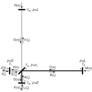
Figure 1: Design for QND speed meter interferometer. The main laser input port is the lower left mirror [denoted by $I(\zeta)$, where $\zeta=t-z/c$]. The signal is extracted at the bottom mirror [denoted $K(\eta)$, where $\eta=t+z/c$]. The “$+$” and “$-$” signs near the mirrors indicate the sign of the reflectivities in the junction conditions for each location.

The basic design of the speed meter to be analyzed here is shown in Figure 1. It consists of two nearly identical optical cavities of length $L=4{\rm km}$, which are weakly coupled by a mirror of power transmissivity $T_{\rm s}$. In the absence of a driving force, laser light can “slosh” back and forth between these two cavities with frequency

$$\Omega=c\sqrt{T_{\rm s}}/L\;,$$ (1)

where $c$ is the speed of light. The addition of a driving laser [denoted $I(\zeta)$ in Fig. 1] into one cavity will cause the other cavity to become excited. It is from this excited cavity that we will extract our signal [denoted $K(\eta)$] at a rate

$$\delta=cT_{\rm o}/4L\;,$$ (2)

where $T_{\rm o}$ is the transmissivity of the extraction mirror. Since we cannot make $T_{\rm o}$ infinitely small (or equivalently, the extraction time infinite), a small amount of residual light will build up in the unexcited cavity. To counteract this, we also input a small amount of laser light [denoted $L(\zeta)$] through the output port in order to cancel out any such residual light. This is desirable because one cavity must be empty to achieve pure speed meter behavior.

To understand how this system produces a velocity signal, consider the effect of moving the end mirror in the excited cavity [the cavity labeled $C(\eta)$ and $B(\zeta)$ in Fig. 1]. That mirror motion will put a phase shift on the light in that cavity. If the input laser is driving the cavity’s cosine quadrature, then the phase shift caused by the mirror motion will act as a driving force for the sine quadrature. This light will then slosh into the empty cavity and back. When it returns, it will be $180^{\circ}$ out of phase compared to its initial phase shift. The resulting cancellation will cause the net signal in the sine quadrature of the excited cavity to be proportional to the difference in test-mass position between the start and finish of the sloshing cycle. In other words, the net signal is proportional to the velocity of the test mass, assuming that the frequencies $\omega$ of the test mass’ motion are $\omega\ll\Omega$.

As it turns out, however, the optimal regime of operation for the speed meter is $\omega\sim\Omega$. Consequently, the output signal contains a sum over odd time derivatives of position [see Eq. (47) and the discussion following it]. Therefore, the speed meter monitors not just the relative speed of the test masses, but a mixture of all odd time derivatives of the position.

As we will show, this speed meter design, in principle, is capable of beating the SQL by an arbitrary amount and over a wide range of frequencies. However, in practice, optical losses will limit the amount by which the SQL can be beaten, and to beat the SQL at all requires an uncomfortably high circulating power. (This is actually a common feature of designs that beat the SQL highpower .) More seriously, this design requires an impossibly high input power because the photons are not getting “sucked” into the interferometer efficiently, as they are in conventional designs; this will be discussed in more detail in Sec. III.3.

In view of this impracticality, one might wonder why a detailed analysis of this speed meter should be published. The answer is that this analysis teaches us a variety of things about optical-interferometer speed meters — things that are likely to be of value in the search for practical QND interferometers and in their optimization. Indeed, the author and Yanbei Chen are now exploring more sophisticated and promising speed-meter designs that rely, for motivation and insights, on the things learned in the analysis presented here.

This paper is organized as follows: The mathematical description of the interferometer is given in Sec. II. Sec. III.1 gives the analysis of the lossless limit and the mapping to the microwave-resonator speed meter, Sec. III.2 presents the numerical analysis, and as mentioned above, Sec. III.3 describes various problems or issues with the speed meter. In Sec. IV, we give the results and a description of the speed meter’s performance if losses are included. The discussion there will address the role of optical dissipation in limiting the amount by which the SQL can be beaten. Finally, Sec. V summarizes the results of this analysis and its relevance for future research.

II Mathematical Description of the Interferometer

The design of the speed meter is shown in Figure 1. In this section, we will set up the equations describing the interferometer with lossy mirrors. The method of analysis is based on the formalism developed by Caves and Schumaker cs and used by Kimble, Matsko, Thorne, and Vyatchanin (KLMTV) Kimble to examine more conventional interferometer designs.

We express the electric field propagating in each direction down each segment of the interferometer in the form

$$E_{\rm field}(\zeta)=\sqrt{\frac{4\pi\hbar\omega_{0}}{{\cal S}c}}A(\zeta)\;,$$ (3)

where $A(\zeta)$ is the amplitude, $\zeta=t-z/c$ (see Fig. 1), $\omega_{0}$ is the carrier frequency, $\hbar$ is the reduced Planck’s constant, and ${\cal S}$ is the effective cross-sectional area of the light beam; see Eq. (8) of KLMTV. We decompose the amplitude into cosine and sine quadratures,

$$A(\zeta)={\cal A}_{1}(\zeta)\cos\omega_{0}\zeta+{\cal A}_{2}(\zeta)\sin\omega_{0}\zeta\;.$$ (4)

Note that the subscript 1 always refers to the cosine quadrature, and 2 to sine. Also note that we have designated $z=0$ at both the input and output mirrors, $z=z_{*}$ at the sloshing mirror, and $z=L$ at the end mirrors; see Fig. 1. We choose the cavity lengths $L$ to be exact half multiples of the carrier wavelength so $e^{i2\omega_{0}L/c}=1$.

As mentioned above, the power transmissivity for the sloshing mirror is $T_{\rm s}$ and for the output mirror is $T_{\rm o}$. In addition, $T_{\rm i}$ will denote the transmissivity for the laser-input mirror and $T_{\rm e}$ for the end mirrors; again, see Fig. 1. Each of these has a complementary reflectivity such that each mirror satisfies the equation $T+R=1$. If we now let $\zeta=t-z/c$, $\eta=t+z/c$, and $j=1,2$, then the junction conditions at the mirrors are given by:

$${\cal A}_{j}(\zeta) = \sqrt{T_{\rm o}}{\cal L}_{j}(\zeta)+\sqrt{R_{\rm o}}{\cal D}_{j}(\eta)\;,$$ (5)

$${\cal B}_{j}(\zeta) = \sqrt{T_{\rm s}}{\cal E}_{j}(\zeta)+\sqrt{R_{\rm s}}{\cal A}_{j}(\zeta)\;,$$ (6)

$${\cal C}_{j}(\eta) = \sqrt{T_{\rm e}}{\cal M}_{j}(\eta)+\sqrt{R_{\rm e}}{\cal B}_{j}(\zeta)\;,$$ (7)

$${\cal D}_{j}(\eta) = \sqrt{T_{\rm s}}{\cal G}_{j}(\eta)+\sqrt{R_{\rm s}}{\cal C}_{j}(\eta)\;,$$ (8)

$${\cal E}_{j}(\zeta) = \sqrt{T_{\rm i}}{\cal I}_{j}(\zeta)-\sqrt{R_{\rm i}}{\cal H}_{j}(\eta)\;,$$ (9)

$${\cal F}_{j}(\zeta) = \sqrt{T_{\rm s}}{\cal A}_{j}(\zeta)-\sqrt{R_{\rm s}}{\cal E}_{j}(\zeta)\;,$$ (10)

$${\cal G}_{j}(\eta) = \sqrt{T_{\rm e}}{\cal N}_{j}(\eta)-\sqrt{R_{\rm e}}{\cal F}_{j}(\zeta)\;,$$ (11)

$${\cal H}_{j}(\eta) = \sqrt{T_{\rm s}}{\cal C}_{j}(\eta)-\sqrt{R_{\rm s}}{\cal G}_{j}(\eta)\;,$$ (12)

$${\cal J}_{j}(\eta) = \sqrt{T_{\rm i}}{\cal H}_{j}(\eta)+\sqrt{R_{\rm i}}{\cal I}_{j}(\zeta)\;,$$ (13)

$${\cal K}_{j}(\eta) = \sqrt{T_{\rm o}}{\cal D}_{j}(\eta)-\sqrt{R_{\rm o}}{\cal L}_{j}(\zeta)\;.$$ (14)

II.1 Carrier Light

If we first consider only the carrier in a steady state, we can assume that all the mirrors are stationary and that all of the ${\cal A}_{j}(\zeta)=A_{j}$, ${\cal B}_{j}(\zeta)=B_{j}$, etc. are constant. (We denote the carrier amplitudes by capital Latin letters with a subscript indicating the quadrature.) Then we solve Eqs. (II) simultaneously. We ignore vacuum fluctuation noise since it is unimportant for the carrier light. In addition, we only drive the cosine quadrature, so that

$$L_{2}=I_{2}=0\;.$$ (15)

Thus, all of the sine quadrature terms will be zero. As mentioned above, we want to have as little light as possible in the unexcited cavity, so we apply the condition

$$F_{1}=G_{1}=0\;.$$ (16)

That means the input fed into the output port should be

$$L_{1}=\frac{I_{1}}{4}\sqrt{\frac{T_{\rm o}T_{\rm i}}{T_{\rm s}}}\;.$$ (17)

Then, the solution for the carrier is

$$A_{1}=B_{1}=C_{1} = D_{1}=\frac{I_{1}}{2}\sqrt{\frac{T_{\rm i}}{T_{\rm s}}}\;,$$ (18)

$$E_{1}=H_{1} = \frac{I_{1}}{2}\sqrt{T_{\rm i}}\;.$$ (19)

In deriving Eqs. (II.1), we have assumed the following inequalities among the various mirror transmissivities:

$$T_{\rm o}\gg T_{\rm s}\gg T_{\rm i}\gg T_{\rm e}\;.$$ (20)

The motivations for these assumptions are that: (i) they lead to speed-meter behavior; (ii) as with any interferometer, the best performance is achieved by making the end-mirror transmissivities $T_{\rm e}$ as small as possible; (iii) good performance requires a light extraction rate comparable to the sloshing rate, $\delta\sim\Omega$ [cf. the first paragraph of Sec. III.2], which with Eqs. (1) and (2) implies $T_{\rm o}\sim\sqrt{T_{\rm s}}$ so $T_{\rm o}\gg T_{\rm s}$; and (iv) if the input transmissivity is larger than or of the same order as the sloshing frequency, too much light will be lost during the sloshing cycle, resulting in incomplete cancellation of the position information and degraded performance (hence, we assume $T_{\rm i}\ll T_{\rm s}$).

II.2 Sideband Light

Sidebands are put onto the carrier by the mirror motions and by vacuum fluctuations, as we shall see below. We express the quadrature amplitudes for the carrier plus the side bands in the form

$${\cal A}_{j}(\zeta)=A_{j}+\int_{0}^{\infty}\bigl{[}\tilde{a}_{j}(\omega)e^{-i\omega\zeta}+\tilde{a}_{j}^{\dagger}(\omega)e^{i\omega\zeta}\bigr{]}\frac{d\omega}{2\pi}\;,$$ (21)

where $\tilde{a}_{j}(\omega)$ is the field amplitude for the sideband at frequency $\omega$ in the $j$ quadrature; cf. Eqs. (6)–(8) of KLMTV, where commutation relations and the connection to creation and annihilation operators are discussed. Then most of the junction conditions can easily be broken down into separate expressions for the constant and sideband terms; for example,

$$A_{j} = \sqrt{T_{\rm o}}L_{j}+\sqrt{R_{\rm o}}D_{j}\;,$$ (22)

$$\tilde{a}_{j} = \sqrt{T_{\rm o}}\tilde{\ell}_{j}+\sqrt{R_{\rm o}}\tilde{d}_{j}\;.$$ (23)

The exceptions are Eqs. (7) and (11) because the two end mirrors will change the phase of the sidebands on each bounce. Equation (11) becomes

$$G_{j} = -\sqrt{R_{\rm e}}F_{j}+\sqrt{T_{\rm e}}N_{j}\;,$$ (24)

$$\tilde{g}_{j} = -\sqrt{R_{\rm e}}\tilde{f}_{j}e^{i\beta}+\sqrt{T_{\rm e}}\tilde{n}_{j}\;,$$ (25)

where $\beta=2\omega L/c$ is the phase shift for the sidebands. At this point, we also want to allow mirror motion in order to detect gravitational waves, so we assume that the end mirror of the excited cavity is free to move. As a result, the junction condition there, expressed by Eq. (7), is the most complicated. It becomes

$$C_{j} = \sqrt{R_{\rm e}}B_{j}+\sqrt{T_{\rm e}}M_{j}\;,$$ (26)

$$\tilde{c}_{1} = \sqrt{R_{\rm e}}\tilde{b}_{1}e^{i\beta}-2\sqrt{R_{\rm e}}B_{2}\omega_{0}\tilde{x}/c+\sqrt{T_{\rm e}}\widetilde{m}_{1}\;,$$ (27)

$$\tilde{c}_{2} = \sqrt{R_{\rm e}}\tilde{b}_{2}e^{i\beta}+2\sqrt{R_{\rm e}}B_{1}\omega_{0}\tilde{x}/c+\sqrt{T_{\rm e}}\widetilde{m}_{2}\;,$$ (28)

where $\tilde{x}$ is the Fourier transform of the mirror’s displacement. (We are ignoring the motion of the end mirror of the empty cavity since that will not have a significant effect.)

All of the junction condition equations [Eqs. (II) expressed in the form of Eqs. (21), (II.2), and (II.2)] can be solved simultaneously to get expressions for the carrier and sidebands in each segment of the interferometer. This yields an output [$K(\eta)$] containing an $\omega\tilde{x}$ term, which is the Fourier transform of the end-mirror velocity (relative to the input mirror), aside from a factor of $i$. Since there is no factor $\tilde{x}$ without a multiplying factor $\omega$ in the output, our interferometer is indeed a speed meter, as claimed by BGKT.

One more complication to be addressed is the issue of the back action force on the mirror produced by the fluctuating radiation pressure of the laser beam. The back action is included in $\tilde{x}$ along with the gravitational wave information, as follows.

From KLMTV, Eq. (B18), the back-action force is

$$F_{BA}=\frac{2\delta W_{\rm circ}}{c}\;,$$ (29)

where $\delta W_{\rm circ}$ is the fluctuation in the circulating laser power. To determine this quantity, consider the expression for the circulating power [text above Eq. (B16) in KLMTV]:

$$W_{\rm circ}=\frac{\overline{E^{2}_{\rm int}}}{4\pi}{\cal S}c\;,$$ (30)

where ${\cal S}$ is the effective cross-sectional area of the beam and $\overline{E^{2}_{\rm int}}$ is the time-averaged square of the internal electric field. In our case,

$$E_{\rm int}= \sqrt{\frac{4\pi\hbar\omega_{0}}{{\cal S}c}}\times$$ (31)

$$\quad\Biggl{\{}\cos(\omega_{0}t)\biggl{[}B_{1}+\int_{0}^{\infty}\bigl{(}\tilde{b}_{1}e^{-i\omega t}+\tilde{b}_{1}^{\dagger}e^{i\omega t}\bigr{)}\frac{d\omega}{2\pi}\biggr{]}$$

$$\quad+\sin(\omega_{0}t)\biggl{[}\int_{0}^{\infty}\bigl{(}\tilde{b}_{2}e^{-i\omega t}+\tilde{b}_{2}^{\dagger}e^{i\omega t}\bigr{)}\frac{d\omega}{2\pi}\biggr{]}\Biggr{\}}\;.$$

See Eqs. (3), (4), and (21) with $\cal A$ replaced by $\cal B$. Note that the constant term $B_{2}$ vanishes since we are driving only the cosine quadrature. Substituting Eq. (31) into Eq. (30) will give a steady circulating power

$$W_{\rm circ}=\frac{1}{2}\hbar\omega_{0}B_{1}^{2}=\hbar\omega_{0}I_{1}^{2}\frac{T_{\rm i}}{8T_{\rm s}}$$ (32)

and a fluctuating piece

$$\delta W_{\rm circ}(t)=\hbar\omega_{0}B_{1}\int_{0}^{\infty}\tilde{b}_{1}(\omega)e^{-i\omega t}\frac{d\omega}{2\pi}+{\rm HC}\;,$$ (33)

where HC denotes the Hermitian conjugate of the previous term.

Now that we have an expression for $\delta W_{\rm circ}$, we return to the expression for the back-action force (29). That force, together with the gravitational waves, produces a relative acceleration of the cavity’s two mirrors (each with mass $m$) given by

$$\frac{d^{2}x(t)}{dt^{2}}=\frac{1}{2}L\frac{d^{2}h(t)}{dt^{2}}+\frac{4\delta W_{\rm circ}(t)}{mc}$$ (34)

where $h(t)$ is the gravitational-wave field [cf. Eq. (B19) in KLMTV]. Substituting Eq. (33) into the above equation and taking the Fourier transform gives

$$\tilde{x}=\frac{1}{2}L\tilde{h}-\frac{4\hbar\omega_{0}B_{1}\tilde{b}_{1}}{mc\omega^{2}}\;.$$ (35)

Here $B_{1}$ is given by Eq. (18), and $\tilde{b}_{1}$, as obtained by solving the junction conditions and simplifying with the conditions on the transmissivities (20), is given by

$$\tilde{b}_{1}=\frac{-i\omega c\sqrt{T_{\rm o}}\tilde{\ell}_{1}}{2L{\cal L}(\omega)}\;,$$ (36)

where

$${\cal L}(\omega)=\Omega^{2}-\omega^{2}-i\omega\delta\;.$$ (37)

(Recall that $\Omega=c\sqrt{T_{\rm s}}/L$ is the sloshing frequency, $\delta=cT_{\rm o}/4L$ the extraction rate.)

III Speed Meter in the Lossless Limit

III.1 Mathematical Analysis

For simplicity, in this section we will set $T_{\rm e}=0$ (end mirrors perfectly reflecting), since it is unimportant if $T_{\rm e}$ is much smaller than the other transmissivities. We will also neglect the noise coming in the main laser port ($\tilde{i}_{1,2}$). This noise will become dominant at sufficiently low frequencies (below $\sim$10 Hz for the interesting parameter regime), but those frequencies are not very relevant to LIGO.

As a result of these assumptions, the only noise that remains is that which comes in through the output port ($\tilde{\ell}_{1,2}$). An interferometer in which this is the case and in which light absorption and scattering are unimportant ($R+T=1$ for all mirrors, as we have assumed) is said to be “lossless.” In Sec. IV, we shall relax these assumptions; i.e. we shall consider lossy interferometers. As before, we assume $T_{\rm o}\gg T_{\rm s}\gg T_{\rm i}$. The interferometer output, as derived by the analysis of the previous section, is then

$$\tilde{k}_{1} = -{{\cal L}^{*}(\omega)\over{\cal L}(\omega)}\tilde{\ell}_{1}\;,$$ (38)

$$\tilde{k}_{2} = \frac{-i\omega\omega_{0}I_{1}\sqrt{T_{\rm o}T_{\rm i}}}{2L\sqrt{T_{\rm s}}{\cal L}(\omega)}\tilde{x}-\frac{{\cal L}^{\ast}(\omega)}{{\cal L}(\omega)}\tilde{\ell}_{2}\;,$$ (39)

where the asterisk (in ${\cal L}^{\ast}(\omega)$) denotes the complex conjugate. Note that $\tilde{x}$ is given by Eq. (35) combined with Eqs. (18) and (36), or equivalently, by

$$\tilde{x}=\frac{1}{2}L\tilde{h}+\tilde{x}_{\rm BA}\;,$$ (40)

where

$$\tilde{x}_{\rm BA}=\frac{i\hbar\omega_{0}I_{1}\sqrt{T_{\rm o}T_{\rm i}}\tilde{\ell}_{1}}{m\omega L\sqrt{T_{\rm s}}{\cal L}(\omega)}$$ (41)

is the back-action noise. It is possible to express Eqs. (III.1) in a more concise form, similar to Eqs. (16) in KLMTV:

$$\tilde{k}_{1} = \tilde{\ell}_{1}e^{2i\psi}\;,$$ (42)

$$\tilde{k}_{2} = (\tilde{\ell}_{2}-\kappa\tilde{\ell}_{1})e^{2i\psi}+\sqrt{\kappa}\frac{\tilde{h}}{h_{SQL}^{\rm conv}}e^{i\psi}\;,$$ (43)

where

$$\tan\psi = -\frac{\Omega^{2}-\omega^{2}}{\omega\delta}\;,$$ (44)

$$\kappa = \frac{\hbar\omega_{0}^{2}I_{1}^{2}T_{\rm o}T_{\rm i}}{2mL^{2}T_{\rm s}|{\cal L}(\omega)|^{2}}\;,$$ (45)

and

$$h_{SQL}^{\rm conv}=\sqrt{\frac{8\hbar}{m\omega^{2}L^{2}}}\;.$$ (46)

If, as in KLMTV, we regard Eqs. (III.1) as input-output relations for the interferometer, then $\kappa$ is a dimensionless coupling constant, which couples the gravity wave signal $\tilde{h}$ into the output $\tilde{k}_{2}$, $\tilde{h}_{SQL}^{\rm conv}$ is the standard quantum limit for a conventional interferometer such as LIGO-I, and $\psi$ and $\varphi$ are phases put onto the signal and noise by the interferometer. Although there is much similarity between the above equations (III.1) and those of KLMTV, there is not a direct mapping because KLMTV analyzes a position meter, not a speed meter.

As a tool in optimizing the interferometer’s performance, we perform homodyne detection on the outputs $\tilde{k}_{1}$ and $\tilde{k}_{2}$, using a constant (frequency-independent) homodyne angle $\Phi$. In other words, we read out $\tilde{k}_{\Phi}=\tilde{k}_{1}\cos\Phi+\tilde{k}_{2}\sin\Phi$. If we insert Eqs. (III.1) and do some algebra, we get:

$$\tilde{k}_{\Phi}=\frac{-i\omega\omega_{0}I_{1}\sqrt{T_{\rm o}T_{\rm i}}}{2L\sqrt{T_{\rm s}}{\cal L}(\omega)}\sin\Phi[\tilde{x}(\omega)+\tilde{x}_{m}(\omega)]\;.$$ (47)

Here $\tilde{x}_{m}$, the measurement noise (actually shot noise), is given by

$$\tilde{x}_{m}={2L\sqrt{T_{\rm s}}{\cal L}^{*}(\omega)\over i\omega\omega_{0}I_{1}\sqrt{T_{\rm o}T_{\rm i}}}[\tilde{\ell}_{2}+\tilde{\ell}_{1}\cot\Phi]\;,$$ (48)

and $\tilde{x}$ is given by Eqs. (40) and (41). Notice that the first term in Eq. (47) contains $\tilde{x}$ only in the form $\omega\tilde{x}$; this is the velocity signal [actually, the sum of the velocity and higher odd time derivatives of position because of the ${\cal L}(\omega)$ in the denominator]. These equations, (47) and (48), are equivalent to Eqs. (29) and (30) of BGKT. In fact, the analysis of the single-test-mass, microwave speed meter in that reference (Sec. III.3) can be translated more or less directly into the analysis of our speed-meter interferometer with a suitable change of notation (see Table 1).

Table 1: Mapping of the parameters in the BGKT microwave-resonator speed meter paper to those in this paper.

Parameter	BGKT	Purdue
signal frequency	$\omega$	$\omega$
carrier frequency	$\omega_{e}$	$\omega_{0}$
optimal frequency	$\omega_{0}$	$\omega_{\rm opt}$
mass of test body	$m$	$m$
characteristic length	$d$	$L$
sloshing frequency	$\Omega$	$\Omega=c\sqrt{T_{\rm s}}/L$
test-mass displacement	$\tilde{x}(\omega)$	$\tilde{x}(\omega)$
signal extraction rate	$\delta_{e}=1/2\tau_{e}^{\ast}$	$\delta=cT_{\rm o}/4L$
impedance of resonators	$\rho$	$\rho_{\rm o}=2L/c\sqrt{T_{\rm o}}$
		$\rho_{\rm i}=2L/c\sqrt{T_{\rm i}}$
driving amplitude	$U_{0}$	$\alpha I_{1}$
amp. in excited cavity	$-q_{0}=U_{0}/\Omega\rho$	$\alpha B_{1}=\alpha I_{1}/\Omega\rho_{\rm i}$
noise into output port,	$\{U_{es},\ U_{ec}\}$	$-\alpha\{\tilde{\ell}_{1},\ \tilde{\ell}_{2}\}$
sideband components,	$\{a_{1},b_{1},a_{2},b_{2}\}$	$\alpha\{\tilde{b}_{1},\tilde{b}_{2},\tilde{f}_{1},\tilde{f}_{2}\}$
output amplitude	$\tilde{U}(\omega)$	$\alpha\tilde{k}_{\Phi}(\omega)$

We assume that ordinary vacuum enters the output port of the interferometer; i.e. $\tilde{\ell}_{1}$ and $\tilde{\ell}_{2}$ are quadrature amplitudes for ordinary vacuum. This means [Eq. (26) of KLMTV] that their spectral densities are unity and their cross-correlations are zero. By noting that the homodyne output (47) is proportional to

$$\frac{2}{L}(\tilde{x}+\tilde{x}_{m})=\tilde{h}+\frac{2}{L}(\tilde{x}_{BA}+\tilde{x}_{m})$$ (49)

and examining the dependence of $\tilde{x}_{BA}$ and $\tilde{x}_{m}$ on the input vacuum $\tilde{\ell}_{1}$ and $\tilde{\ell}_{2}$, we deduce the (single-sided) spectral density of the gravitational wave output noise $\tilde{h}$:

$$S_{h_{n}}=(h_{SQL}^{\rm speed})^{2}\xi^{2}\;,$$ (50)

where

$$h_{SQL}^{\rm speed}=\sqrt{\frac{16\hbar}{m\omega^{2}L^{2}}}\;,$$ (51)

is the standard quantum limit (SQL) for our speed-meter interferometer,

$$\xi^{2}={|{\cal L}(\omega)|^{2}\over 2\Lambda^{4}\sin^{2}\Phi}-\cot\Phi+{\Lambda^{4}\over 2|{\cal L}(\omega)|^{2}}\;,$$ (52)

is the fractional amount by which the SQL is beaten (in units of squared amplitude), and

$$\Lambda^{4}={\hbar T_{\rm o}T_{\rm i}(\omega_{0}I_{1})^{2}\over 2L^{2}mT_{\rm s}}\;.$$ (53)

Note that the quantity $\xi^{2}$ is the same (modulo a minus sign in the definition of $\Phi$) as the quantity $\xi^{2}_{\rm WB}$ in BGKT [Eq. (40)].

[We comment, in passing, on the SQLs that appear in the various papers: BGKT use double-sided spectral densities and measure the velocity of a single test body with mass $\mu$. The corresponding standard quantum limit for position is

$$(S_{x,SQL}^{\rm one\ body})_{\rm double\mbox{-}sided}=\frac{\hbar}{\mu\omega^{2}}$$ (54)

[their Eq. (5) divided by $\mu^{2}\omega^{4}$ to convert from force to position and with $\mu$ denoted by $m$]. KLMTV and the present paper used single-sided spectral densities, i.e. we fold negative frequencies into positive, so our one-body SQL is

$$(S_{x,SQL}^{\rm one\ body})_{\rm single\mbox{-}sided}=\frac{2\hbar}{\mu\omega^{2}}\;.$$ (55)

For our speed meter, the quantity measured is the relative velocity of two mirrors, $x=x_{1}-x_{2}$, for which the gravitational-wave signal is $\frac{1}{2}\tilde{h}L$ and the reduced mass is $\mu=m/2$, so our gravity-wave SQL spectral density is

$$(S_{h,SQL}^{\rm speed\ meter} )_{\rm single\mbox{-}sided}\equiv(h_{SQL}^{\rm speed})^{2}$$ (56)

$$=\biggl{(}\frac{2}{L}\biggr{)}^{2}\frac{2\hbar}{(m/2)\omega^{2}}=\frac{16\hbar}{m\omega^{2}L^{2}}\;.$$

For a conventional interferometer, as analyzed by KLMTV, the quantity measured is the relative position of four mirrors, $x=(x_{1}-x_{2})-(x_{3}-x_{4})$, for which the gravitational-wave signal is $2\cdot\frac{1}{2}\tilde{h}L=\tilde{h}L$ and the reduced mass is $\mu=m/4$, so the gravity-wave SQL spectral density is

$$(S_{h,SQL}^{\rm conv} )_{\rm single\mbox{-}sided}\equiv(h_{SQL}^{\rm conv})^{2}$$ (57)

$$=\biggl{(}\frac{1}{L}\biggr{)}^{2}\frac{2\hbar}{(m/4)\omega^{2}}=\frac{8\hbar}{m\omega^{2}L^{2}}\;,$$

half as large as for our speed meter. If we were to build a speed meter consisting of two excited cavities (one in each arm) and two unexcited cavities (as in Fig. 4 of BGKT), then our speed meter SQL would be reduced by a factor of 2, to the same value as for a conventional interferometer.]

Continuing with our analysis, we can express $|{\cal L}(\omega)|^{2}$ [Eq. (37)] as

$$|{\cal L}(\omega)|^{2}=(\omega^{2}-\omega_{\rm opt}^{2})^{2}+\delta^{2}(\omega^{2}_{\rm opt}+\delta^{2}/4)\;,$$ (58)

where

$$\omega_{\rm opt}=\sqrt{\Omega^{2}-\delta^{2}/2}\;,$$ (59)

as we shall see, is the interferometer’s optimal frequency. These two expressions are identical to Eqs. (37) and (38) of BGKT. We shall optimize the homodyne angle $\Phi$ to minimize the noise at some specific frequency, $\omega_{F}$. The result is

$$\cot\Phi={\Lambda^{4}\over|{\cal L}(\omega_{F})|^{2}}\;.$$ (60)

Then, Eqs. (42)–(48) of BGKT apply exactly to the analysis here: $\xi^{2}(\omega)$ for this homodyne phase $\Phi$ (60) is

$$\xi^{2}(\omega)=\frac{|{\cal L}(\omega)|^{2}}{2\Lambda^{4}}+\frac{\Lambda^{4}(\omega^{2}-\omega_{F}^{2})^{2}(\omega^{2}+\omega_{F}^{2}-2\omega_{\rm opt}^{2})^{2}}{2|{\cal L}(\omega)|^{2}|{\cal L}(\omega_{F})|^{4}}\;,$$ (61)

and its minimum is

$$\xi^{2}_{\rm min}=\xi^{2}(\omega_{F})=\frac{(\omega_{F}^{2}-\omega_{\rm opt}^{2})^{2}+\delta^{2}(\omega_{\rm opt}^{2}+\delta^{2}/4)}{2\Lambda^{4}}\;.$$ (62)

The noise can be further minimized by setting the speed meter’s optimal frequency to $\omega_{\rm opt}=\omega_{F}$ to get

$$\xi^{2}(\omega)=\frac{|{\cal L}(\omega)|^{2}}{2\Lambda^{4}}+\frac{\Lambda^{4}(\omega^{2}-\omega_{\rm opt}^{2})^{4}}{2|{\cal L}(\omega)|^{2}\delta^{4}(\omega_{\rm opt}^{2}+\delta^{2}/4)^{2}}\;,$$ (63)

with

$$\xi^{2}_{\rm min}=\frac{\delta^{2}(\omega_{\rm opt}^{2}+\delta^{2}/4)}{2\Lambda^{4}}={W^{\rm SQL}_{\rm circ}\over W_{\rm circ}}\;.$$ (64)

Here $W_{\rm circ}$ is the power circulating in the excited arm [Eq. (32)] and

$$W^{\rm SQL}_{\rm circ} = {mL^{2}\delta^{2}(\omega_{\rm opt}^{2}+\delta^{2}/4)\over 8\omega_{0}T_{\rm o}}$$ (65)

$$= (0.8{\rm MW})\biggl{(}\frac{m}{40{\rm kg}}\biggr{)}\biggl{(}\frac{L}{4{\rm km}}\biggr{)}^{2}\biggl{(}\frac{0.07}{T_{\rm o}}\biggr{)}$$

$$\quad\times\biggl{(}\frac{\omega_{\rm opt}}{2\pi\times 100{\rm Hz}}\biggr{)}^{4}\biggl{(}\frac{1.78\times 10^{15}{\rm Hz}}{\omega_{0}}\biggr{)}$$

is the circulating power required to reach the standard quantum limit at the optimal frequency $\omega_{\rm opt}$ (we have assumed $\delta=2\omega_{\rm opt}$ to get the second line of the above equation; see Sec. III.2). By pumping with a power $W_{\rm circ}>W_{\rm circ}^{\rm SQL}$, the speed meter can beat the SQL in the vicinity of the optimal frequency $\omega_{\rm opt}$ by the amount $\xi_{\rm min}^{2}=W^{\rm SQL}_{\rm circ}/W_{\rm circ}$.

If [following BGKT Eqs. (47) and (48)] we define the frequency band $\omega_{1}<\omega<\omega_{2}$ of high sensitivity to be those frequencies for which

$$\xi(\omega)\leq\sqrt{2}\xi(\omega_{\rm opt})\;,$$ (66)

then Eqs. (63) and (64) imply that

$$\omega_{1,2}^{2} = \omega_{\rm opt}^{2}\mp\frac{\delta^{2}(\omega_{\rm opt}^{2}+\delta^{2}/4)}{\sqrt[4]{\delta^{4}(\omega_{\rm opt}^{2}+\delta^{2}/4)^{2}+\Lambda^{8}}}$$ (67)

$$= \omega_{\rm opt}^{2}\mp\frac{2\Lambda^{2}\xi_{\rm min}^{2}}{\sqrt[4]{4\xi_{\rm min}^{4}+1}}\;.$$

Equations (67), (63), and (64) imply that the lossless speed meter can beat the force-measurement SQL by a large amount $\xi_{\rm min}\ll 1$ over a wide frequency band, $\omega_{1}\ll\omega_{2}\sim\sqrt{2}\omega_{\rm opt}$ by setting

$$\frac{\Lambda}{\omega_{\rm opt}}\sim\frac{\delta^{2}}{2\omega_{\rm opt}^{2}}\gtrsim 2\;.$$ (68)

A plot of $\xi^{2}$, optimized in this manner but for rather modest parameter values, is shown in Fig. 2.

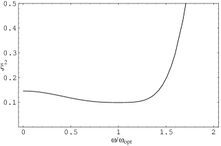
Figure 2: Plot of the squared amount by which the speed meter beats the standard quantum limit ($h_{SQL}^{\rm speed}$), as a function of frequency (normalized to the optimal frequency, $\omega_{\rm opt}$). For the parameter values $\xi_{\rm min}^{2}=0.1$, $\delta=2\omega_{\rm opt}$, and $\Lambda^{4}=40\omega_{\rm opt}^{4}$, this is identical to the speed meter curve in Fig. 3 of BGKT.

III.2 Numerical Analysis

To get an idea of the magnitudes of the quantities involved in this interferometer, we can start by combining the wide-bandwith requirement (68) with the definitions $\delta=cT_{\rm o}/4L$, $\Omega=c\sqrt{T_{\rm s}}/L$, and $\omega_{\rm opt}^{2}=\Omega^{2}-\delta^{2}/2$. From these, we find that the wide-bandwidth requirement $\delta^{2}\gtrsim 4\omega_{\rm opt}^{2}$ becomes $T_{\rm o}^{2}\gtrsim(64/3)T_{\rm s}$. If, as in BGKT, we take $\delta=2\omega_{\rm opt}=2\omega_{F}$ but set $\omega_{\rm opt}=2\pi\times 100{\rm Hz}$ as in KLMTV, then that gives $T_{\rm o}=0.07$ and $T_{\rm s}=0.0002$. Notice this particular value of $T_{\rm s}$ does not satisfy the condition $\omega_{\rm opt}\ll\Omega$, which was necessary to get a signal that is only proportional to the velocity of the test masses’ motion. Instead, we have $\omega_{\rm opt}\sim\Omega$, which implies that the signal consists of a linear combination of odd time derivatives of position, with substantial contributions coming from derivatives higher than the speed [see Eq. (47)].

If, in addition to $\delta=2\omega_{\rm opt}=2\omega_{F}=4\pi\times 100{\rm Hz}$, we choose $\xi_{\rm min}^{2}=0.1$ (as in BGKT), then we find $W_{\rm circ}^{SQL}\simeq 0.8\ {\rm MW}$ from Eq. (65) and a circulating power of $W_{\rm circ}\simeq 8\ {\rm MW}$. The input-port transmissivity is not explicitly defined by the above requirements, but it is required, in our analysis, to be much smaller than $T_{\rm s}=0.0002$ or $T_{\rm o}=0.07$, i.e. $T_{\rm i}\lesssim 2\times 10^{-5}$. This then dictates an outrageously high input power of $\gtrsim$300 MW to get the needed circulating power. The power that exits through the signal port, along with the signal, is $W_{\rm exit}=T_{\rm o}W_{\rm circ}\sim 0.56\ {\rm MW}$. The resulting noise curve is shown in Fig. 3; the parameter values used are given in Table 2.

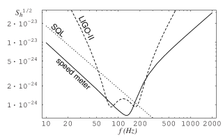
Figure 3: Lossless noise curve for a speed meter optimized at a frequency of 100 Hz. The transmissivities and power are given in Table 2. The dashed line represents the theoretical LIGO-II noise curve in which a signal-recycling mirror and optical noise correlations have been used to beat the SQL (and thermal noise has been made negligible), as described by Buonanno and Chen SRrefa ; SRrefb . The dotted line represents the SQL; we use $h_{SQL}^{\rm conv}$ because we are comparing to a position meter.

Table 2: Interferometer parameters and their fiducial values.

Parameter	Symbol	Fiducial Value
carrier frequency	$\omega_{0}$	$1.78\times 10^{15}{\rm s}^{-1}$
mirror mass	$m$	40 kg
arm length	$L$	4 km
sloshing mirror transmissivity	$T_{\rm s}$	0.0002
input mirror transmissivity	$T_{\rm i}$	$2\times 10^{-5}$
output mirror transmissivity	$T_{\rm o}$	0.07
end mirror transmissivity	$T_{\rm e}$	$2\times 10^{-6}$
SQL circulating power	$W_{\rm circ}^{SQL}$	1.7 MW

Recall that this analysis is for only one speed meter, which is equivalent to a single arm of the conventional LIGO design. If we were to add another speed meter (another pair of cavities) with the position of the excited and unexcited cavities reversed, interfering the output beams would increase the sensitivity by a factor of two, in much the same way as having two arms increases the sensitivity in the conventional LIGO design. In addition, doing this would reduce the interferometer’s sensitivity to laser frequency fluctuations in the same way as having two arms in conventional LIGO designs.

III.3 Discussion of Lossless Speed Meter

In this section, we will look at variety of issues that should be understood and addressed in the process of developing a different, more practical, speed-meter design. One problem is the large circulating power ($\sim$8 MW) required to achieve wide-band sensitivity a factor $\sim 10$ in noise power below the standard quantum limit. A second problem is how to get that light into the interferometer, as the present design requires an input power that is outrageously high. This is, at least partly, the result of the high reflectivity of the input mirror, which causes most of the input light to be reflected back towards the laser.

A third problem is the amount of power flowing through the interferometer: With a circulating power of $\sim$8 MW, the power extracted with the signal is $W_{\rm exit}=T_{\rm o}W_{\rm circ}\sim 0.56\ {\rm MW}$. This same amount of power must be fed into the excited cavity to maintain a steady state. To reduce this power through-put, we could decrease $T_{\rm o}$ substantially; however, doing this will cause the wide-bandwidth requirement (68) to be violated, and consequently, the behavior of the speed meter will become more narrow-band. In fact, the effect of changing $T_{\rm o}$ is strong enough that if it is decreased by one order of magnitude, the speed meter will no longer beat the SQL except for a very narrow range of frequencies. This clearly is not a viable solution.

Another approach, in which this large through-put power might conceivably be tolerated, is to recycle it back into the interferometer. To do that, we must strip the signal off by using a beamsplitter to interfere the outputs from two speed-meter interferometers as in Fig. 4 of BGKT. Using this “double” speed meter could also help increase the sensitivity, as described at the end of the previous section.

Turning to the issue of the high circulating power, it should first be noted that the circulating power required to reach the SQL, $W_{\rm circ}^{SQL}\sim 800\ {\rm kW}$ is comparable to that for conventional interferometers [Eq. (132) of KLMTV gives $W_{\rm circ}^{SQL}\sim 840\ {\rm kW}$ with $m=40{\rm kg}$, instead of 30kg]. A double speed meter, as described above, would have twice the sensitivity as a single speed meter at the same power. As mentioned in Sec. I, the high powers needed to reach or beat the SQL are a common feature of many QND designs highpower , for example the variational-output interferometer discussed in KLMTV.

A likely method of reducing the needed circulating power, without losing the wide-band performance of the speed meter, is to inject squeezed vacuum into the output port, as was originally proposed by Caves Cavessqueezedvacuum for conventional interferometers and by KMLTV for their QND squeezed-input and squeezed-variational interferometers. In these cases, for realistic amounts of squeezing, the circulating power can be reduced by as much as an order of magnitude Cavessqueezedvacuum ; Kimble . Detailed analyses applying squeezed-vacuum techniques to speed meters have not yet been carried out, but if the effect is similar, it would have the beneficial side-effect of reducing the needed input power by the same amount, which might be useful in a redesigned speed meter.

As for the outrageously high input power, the fact that so much of the light impinging on the input-port mirror is reflected back to the laser suggests an obvious solution would be adding a power-recycling mirror and/or increasing the transmissivity $T_{\rm i}$ of the input mirror. However, neither of these approaches addresses the fundamental problem: there is an empty cavity between the driving laser and the excited cavity. In a conventional LIGO-type interferometer, the laser drives a strongly excited Fabry-Perot cavity directly. In that case, Bose statistics dictate that photons will be “sucked” into the cavities, producing a strong amplification. Hence, there will be significantly more power stored in the arms of the interferometer than the driving laser is producing. Without losses,

$$\frac{\rm circulating\ power}{\rm input\ power}\sim\frac{8}{T_{\rm PR}T_{\rm IM}}\sim 10^{5}\;,$$ (69)

where $T_{\rm PR}\sim 0.06$ is the transmissivity of the power-recycling mirror and $T_{\rm IM}\sim 0.005$ is that of the internal mirrors LIGOIIdoc . However, in this speed meter design, there is an empty cavity instead of a low power laser feeding into the highly-excited cavity so Bose statistics do not help us. The result is the need for a driving laser that produces far more power than is stored in the arms of the speed meter:

$$\frac{\rm circulating\ power}{\rm input\ power}\sim\frac{T_{\rm i}}{4T_{\rm s}}\sim 10^{-3}\;.$$ (70)

One way to address this problem would be to allow a small amount of light to build up in the previously empty cavity. This would cause position information to contaminate the previously pure speed meter behavior. However, this solution is not ideal because, as the amount of light in the “empty” cavity increases, the sensitivity degrades faster than the required input power decreases. To consider this more closely, we first need to remove the restriction (17) on the light $L_{1}$ fed into the output port, which forces the unexcited cavity [denoted by $F(\zeta)$ and $G(\eta)$ in Fig. 1] to be truly empty. Instead, we let $L_{1}$ be determined by the amount of power we want to have in the unexcited cavity. Secondly, since the unexcited cavity is no longer empty, we need to include the movement of the end mirror in that cavity, which we previously neglected. This requires revising Eqs. (II.2) to include $\tilde{x}$ terms (with back action) as in Eqs. (II.2). To calculate how much the needed input power decreases as a function of the ratio of the powers of the two cavities, we can solve for the carrier, as in Eqs. (II.1), and do some algebra to express the input amplitude $I_{1}$ as a function of the excited-cavity amplitude $B_{1}$ and the ratio of the amplitudes of the powers of the two cavities ($F_{1}/B_{1}$). After converting from amplitudes to powers, the relationship between the input powers is

$${W_{\rm input}(R)\over W_{\rm input}(R=0)}=\Biggl{[}1-\frac{T_{\rm i}\sqrt{R}}{2\sqrt{T_{\rm s}}}\Biggr{]}\;,$$ (71)

where $R$ is the ratio of the powers in the two cavities. Since we require $T_{\rm i}\ll T_{\rm s}\ll 1$ and $R\ll 1$ to get speed-meter behavior, $W_{\rm input}$ cannot be reduced much at all.

Also of concern here is how much position information will be included in the output. To calculate the strength of the position signal, relative to the strength of the velocity signal, we can solve the revised equations (as described in the previous paragraph) for the sideband-light output. Then taking the ratio of the coefficients of the position $\tilde{x}$ term and the velocity $\tilde{x}$ term, we find

$$\Bigl{|}\frac{\rm position}{\rm velocity}\Bigr{|}\sim\frac{c\sqrt{T_{\rm s}}}{\omega L}\sqrt{R}=\frac{\Omega}{\omega}\sqrt{R}\sim\sqrt{R}\;.$$ (72)

Since the spectral density involves the square of the amplitudes used to calculate the above expression (72), $S_{h_{n}}$ and $\xi^{2}$ will scale with $R$. This indicates that even a modest amount of power in the ‘empty’ cavity will introduce a significant amount of position information into the output signal. The effect of this, for a few values of $R$, can be seen in Fig. 4.

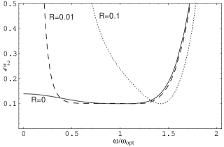
Figure 4: Plot of $\xi^{2}$ for the lossless speed meter optimized at a frequency of 100 Hz, with varying amounts of power in the ‘empty’ cavity. The $R=0$ curve is the same as that in Fig. 2. Transmissivities are $T_{\rm s}=0.0002$, $T_{\rm o}=0.07$, $T_{\rm i}=2\times 10^{-5}$, $T_{\rm e}=0$, and the circulating power is 17 MW.

In fact, it appears that this problem of outrageously high input power is the fatal flaw of this particular speed-meter design. Yanbei Chen altspeedmeter has conceived a class of alternative speed meter designs that may solve this problem. Chen and the author are carrying out an analysis and optimization of them; we shall report the details in a future paper.

IV Sensitivity of Speed Meter with Losses

In order to understand the issue of optical losses and dissipation in this type of interferometer, we shall return to the full equations presented in Sec. II. In that case, the output of the system is:

$$\tilde{k}_{1} = -{{\cal L}^{*}(\omega)\over{\cal L}(\omega)}\tilde{\ell}_{1}+{c^{2}\sqrt{T_{\rm s}T_{\rm o}T_{\rm i}}\over 2L^{2}{\cal L}(\omega)}\tilde{i}_{1}$$ (73)

$$\quad-{i\omega c\sqrt{T_{\rm o}T_{\rm e}}\over 2L{\cal L}(\omega)}\widetilde{m}_{1}+{c^{2}\sqrt{T_{\rm s}T_{\rm o}T_{\rm e}}\over 2L^{2}{\cal L}(\omega)}\tilde{n}_{1}\;,$$

$$\tilde{k}_{2} = \frac{-i\omega\omega_{0}I_{1}\sqrt{T_{\rm o}T_{\rm i}}}{2L\sqrt{T_{\rm s}}{\cal L}(\omega)}\tilde{x}-\frac{{\cal L}^{\ast}(\omega)}{{\cal L}(\omega)}\tilde{\ell}_{2}+\frac{c^{2}\sqrt{T_{\rm s}T_{\rm o}T_{\rm i}}}{2L^{2}{\cal L}(\omega)}\tilde{i}_{2}$$ (74)

$$\quad-\frac{i\omega c\sqrt{T_{\rm o}T_{\rm e}}}{2L{\cal L}(\omega)}\widetilde{m}_{2}+\frac{c^{2}\sqrt{T_{\rm s}T_{\rm o}T_{\rm e}}}{2L^{2}{\cal L}(\omega)}\tilde{n}_{2}\;,$$

where

$$\tilde{x}=\frac{1}{2}L\tilde{h} + \frac{\hbar\omega_{0}I_{1}}{m\omega^{2}L^{2}{\cal L}(\omega)}\Biggl{[}\frac{i\omega L\sqrt{T_{\rm o}T_{\rm i}}}{\sqrt{T_{\rm s}}}\tilde{\ell}_{1}-cT_{\rm i}\tilde{i}_{1}$$ (75)

$$\quad\quad+\frac{i\omega L\sqrt{T_{\rm i}T_{\rm e}}}{\sqrt{T_{\rm s}}}\widetilde{m}_{1}-c\sqrt{T_{\rm i}T_{\rm e}}\tilde{n}_{1}\Biggr{]}\;.$$

As before, we can express these in a more concise way:

$$\tilde{k}_{1} = \tilde{\ell}_{1}e^{2i\psi}-(\tilde{i}_{1}\kappa_{i}+\tilde{n}_{1}\kappa_{n})e^{i\theta}+\widetilde{m}_{1}\kappa_{m}e^{i\psi}\;,$$ (76)

$$\tilde{k}_{2} = \bigl{(}\tilde{\ell}_{2}-\kappa\tilde{\ell}_{1}-\kappa\frac{\sqrt{T_{\rm e}}}{\sqrt{T_{\rm o}}}\widetilde{m}_{1}\bigr{)}e^{2i\psi}-(\tilde{i}_{2}\kappa_{i}+\tilde{n}_{2}\kappa_{n})e^{i\theta}$$ (77)

$$\quad+\biggl{(}\frac{\sqrt{\kappa}}{h_{SQL}^{\rm conv}}\tilde{h}+\kappa_{m}\widetilde{m}_{2}\biggr{)}e^{i\psi}$$

$$\quad+\biggl{(}\tilde{i}_{1}\sqrt{T_{\rm i}}+\frac{\sqrt{T_{\rm e}}}{\sqrt{T_{\rm o}}}\tilde{n}_{1}\biggr{)}\frac{\Omega}{\omega}\kappa e^{i\phi}\;,$$

where, in addition to the definitions given by Eqs. (III.1),

$$\tan\theta=-\cot\psi\;,\quad\tan\phi=-\cot 2\psi\;,$$ (78)

and

$$\kappa_{i} = \sqrt{\frac{c^{4}T_{\rm s}T_{\rm o}T_{\rm i}}{4L^{4}|{\cal L}(\omega)|^{2}}}\;,$$ (79)

$$\kappa_{m} = \sqrt{\frac{c^{2}T_{\rm o}T_{\rm e}\omega^{2}}{4L^{2}|{\cal L}(\omega)|^{2}}}\;,$$ (80)

$$\kappa_{n} = \sqrt{\frac{c^{4}T_{\rm s}T_{\rm o}T_{\rm e}}{4L^{4}|{\cal L}(\omega)|^{2}}}\;.$$ (81)

Once again, we do homodyne detection and calculate the spectral density of the noise. (It should be noted that, in the lossy case, there are enough differences between the optical speed meter and the BGKT microwave speed meter to obscure the mapping. Consequently, we will not be able to present as close a comparison in this section as we did in the lossless case.) The fractional amount by which the SQL is beaten is

$$\xi^{2}={|{\cal L}^{\prime}(\omega)|^{2}\over 2\Lambda^{4}\sin^{2}\Phi}-\cot\Phi+{\Lambda^{4}\over 2|{\cal L}(\omega)|^{2}}\;,$$ (82)

where

$$|{\cal L}^{\prime}(\omega)|^{2}=(\omega^{2}-\omega^{\prime 2}_{\rm opt})^{2}+\delta\delta^{*}[\omega^{\prime 2}_{\rm opt}+\frac{\delta\delta^{\prime}}{4\delta^{*}}(\delta^{*}+\delta_{e}+\delta_{i})]\;,$$ (83)

with

$$\delta_{i} = cT_{\rm i}/L\;,$$ (84)

$$\delta_{e} = cT_{\rm e}/L\;,$$ (85)

$$\delta^{\prime} = \delta+\delta_{e}\;,$$ (86)

$$\delta^{*} = \delta+2\delta_{e}+\delta_{i}\;,$$ (87)

and

$$\omega^{\prime}_{\rm opt}=\sqrt{\Omega^{2}-\delta\delta^{\prime}/2}\;.$$ (88)

Optimizing the homodyne angle at frequency $\omega_{F}$ gives

$$\cot\Phi={\Lambda^{4}\over|{\cal L}^{\prime}(\omega_{F})|^{2}}\;.$$ (89)

The resulting $\xi^{2}$ is

$$\xi^{2}={|{\cal L}^{\prime}(\omega)|^{2}\over 2\Lambda^{4}}-{\Lambda^{4}\over|{\cal L}^{\prime}(\omega_{F})|^{2}}+{\Lambda^{4}|{\cal L}^{\prime}(\omega)|^{2}\over 2|{\cal L}^{\prime}(\omega_{F})|^{2}}+{\Lambda^{4}\over 2|{\cal L}(\omega)|^{2}}\;.$$ (90)

Setting $\omega=\omega_{\rm opt}^{\prime}=\omega_{F}$ gives

$$\xi^{2}(\omega_{\rm opt}^{\prime})= {\delta^{2}\delta^{\prime}(\delta_{e}+\delta_{i})/4+\delta\delta^{*}(\omega_{\rm opt}^{\prime 2}+\delta\delta^{\prime}/4)\over 2\Lambda^{4}}$$ (91)

$$-{\Lambda^{4}\over 2[\delta^{2}\delta^{\prime}(\delta_{e}+\delta_{i})/4+\delta\delta^{*}(\omega_{\rm opt}^{\prime 2}+\delta\delta^{\prime}/4)]}$$

$$+{\Lambda^{4}\over 2[(\omega_{\rm opt}^{\prime 2}-\omega_{\rm opt}^{2})^{2}+\delta^{2}(\omega_{\rm opt}^{2}+\delta^{2}/4)]}\;.$$

Cf. Eq. (64). Note that, as in BGKT, the sensitivity in the lossy case does not continue to grow indefinitely with the growth of the parameter $\Lambda$.

Despite the presence of the additional terms included to account for losses, the speed meter curve is largely unchanged if we maintain our assumptions about the relative sizes of the transmissivities (20). In fact, the only losses that contribute significantly are those associated with $\tilde{i}_{1}$ (i.e., noise entering the bright port along with the laser light). This term causes the speed meter to become less sensitive at frequencies $\ll\omega_{\rm opt}$, as seen in Fig. 5. Since that is roughly the frequency at which seismic noise becomes dominant, the effect of more limited sensitivity in that range is not important.

Figure 5: Plot of $\xi^{2}$ for the speed meter with losses. The solid curve uses the transmissivities given in Table 2. The lossless curve has $T_{\rm e}=0$, as in Fig. 2. The other two curves differ from the fiducial-value curve only by the specified transmissivities.

As it turns out, the equations in this section are valid into the regime where $T_{\rm e}\simeq T_{\rm i}\simeq T_{\rm s}$. In that case, the $\tilde{n}_{1}$ term will be the same size as the $\tilde{i}_{1}$ term, and together, they become dominant at frequencies $\lesssim\omega_{\rm opt}$, while the rest of the loss terms continue to be insignificant for this parameter regime. Presumably, the sensitivity degradation by $\tilde{n}_{1}$ and $\tilde{i}_{1}$ are the result of vacuum fluctuations entering into the empty cavity and contaminating the ‘sloshing’ light. This behavior is shown in Fig. 5. As can be seen from that plot, the interferometer loses wideband sensitivity when operating in this regime.

V Conclusions

We have analyzed the speed-meter interferometer proposed by BGKT and have shown that it does, indeed, measure test-mass speed (and time derivatives of speed) rather than test-mass position. We have also shown that it is capable of beating the SQL over a broad range of frequencies. However, the very high circulating and input powers it requires render this design impractical for use in LIGO-III. It is possible, however, that there are variations of this design that will be more feasible.

There are three separate but related problems related to the laser power involved in this speed meter. One is the amount of circulating power ($\sim$8 MW) required to beat the SQL substantially (by a factor 10 in noise power) over a wide range of frequencies. Another is the amount of power coming out of the interferometer with the signal ($\sim$0.56 MW). Both of these are serious problems, but there are conceivable solutions to them. The third and most severe problem is the fact that the excited cavity is being fed through an empty cavity. This dramatically increases the amount of input power needed to achieve a given circulating power, to the point where the input is significantly greater than the circulating power.

Motivated by what we have learned in this analysis, Yanbei Chen and the author are developing and exploring alternative designs for speed-meter interferometers that may solve the above problems and actually be practical.

References

- (1) A. Abramovici et al., Science 256, 325 (1992).
- (2) B. C. Barish and R. Weiss, Physics Today 52 (10), 44 (1999).
- (3) B. Caron et al., Class. Quantum Grav. 14, 1461 (1997).
- (4) H. Lück and the GEO600 Team. Class. Quantum Grav. 14, 1471 (1997).
- (5) E. Gustafson, D. Shoemaker, K. Strain, and R. Weiss, LSC White Paper on Detector Research and Development, LIGO document T990080-00-D (1999); available along with other relevant information at http://www.ligo.caltech.edu/ligo2/ .
- (6) Although there as yet are no detailed papers on EURO (or LIGO-III), they are much discussed within the gravitational-wave community and at conferences on long-range plans for gravitational-wave detection; see, e.g., the talk by A. Rüdiger at http://www.ligo.caltech/veronica/Aspen2001/ .
- (7) K. Kuroda et al., Large-scale Cryogenic Gravitational-wave Telescope, Int. J. Mod. Phys. D 8, 577 (1999); available at http://www.icrr.u-tokyo.ac.jp/gr/LCGT.pdf .
- (8) C. M. Caves, Phys. Rev. Lett. 45, 75 (1980).
- (9) W. G. Unruh, in Quantum Optics, Experimental Gravitation, and Measurement Theory, eds. P. Meystre and M. O. Scully (Plenum, 1982), p. 647.
- (10) M. T. Jaekel and S. Reynaud, Europhys. Lett. 13, 301 (1990).
- (11) C. M. Caves, Phys. Rev. D 23, 1693 (1981).
- (12) S. P. Vyatchanin and A. B. Matsko, JETP 77, 218 (1993) [Zh. Eksp. Teor. Fiz. 104, 2668 (1993)]; S. P. Vyatchanin and E. A. Zubova, Phys. Lett. A 201, 269 (1995); S. P. Vyatchanin and A. B. Matsko, JETP 82, 1007 (1996) [Zh. Eksp. Teor. Fiz. 109, 1873 (1996)]; ibid. 83, 690 (1996) [Zh. Eksp. Teor. Fiz. 110, 1252 (1996)]; S. P. Vyatchanin, Phys. Lett. A 239, 201 (1998).
- (13) H. J. Kimble, Yu. Levin, A. B. Matsko, K. S. Thorne, and S. P. Vyatchanin, Phys. Rev. D, in press; gr-qc/0008026.
- (14) V. B. Braginsky and F. Ya. Khalily, Phys. Lett. A 218, 167 (1996); V. B. Braginsky, M. L. Gorodetsky, and F. Ya. Khalili, Phys. Lett. A 232, 340 (1997).
- (15) V. B. Braginsky, M. L. Gorodetsky, and F. Ya. Khalili, Phys. Lett. A 246, 485 (1998); quant-ph/9806081.
- (16) A. Buonanno and Y. Chen, submitted to Phys. Rev. D, gr-qc/0107021.
- (17) V. B. Braginsky and F. Ya. Khalili, Phys. Lett. A 257, 241 (1999).
- (18) F. Ya. Khalili, gr-qc/0107084.
- (19) C. M. Caves, K. S. Thorne, R. W. P. Drever, V. D. Sandberg, and M. Zimmermann, Rev. Mod. Phys. 52, 341 (1980); C. M. Caves, in Quantum Optics, Experimental Gravitation, and Measurement Theory, eds. P. Meystre and M. O. Scully (Plenum, 1982), p. 567.
- (20) V. B. Braginsky and F. Ya. Khalili, Phys. Lett. A 147, 251 (1990).
- (21) V. B. Braginsky, M. L. Gorodetsky, F. Ya. Khalili, and K. S. Thorne, Phys. Rev. D 61, 044002 (2000); gr-qc/9906108.
- (22) V. B. Braginsky, M. L. Gorodetsky, F. Ya. Khalili and K. S. Thorne, “Energetic Quantum Limit in Large-Scale Interferometers,” in Gravitational Waves, Proceedings of the Third Edoardo Amaldi Conference, AIP Conference Proceedings Vol. 523, ed. Sydney Meshkov (American Institute of Physics, 2000) pp. 180–192; gr-qc/9907057.
- (23) C. M. Caves and B. L. Schumaker, Phys. Rev. A 31, 3068 (1985); B. L. Schumaker and C. M. Caves, Phys. Rev. A 31, 3093 (1985).
- (24) P. Fritschel, ed., Advanced LIGO Systems Design, LIGO document T010075-00-D (2001); see also http://www.ligo.caltech.edu/ligo2/ .
- (25) Y. Chen (private communication).
- (26) A. Buonanno and Y. Chen, Class. Quantum Grav. 18, L95 (2001); gr-qc/0010011.
- (27) A. Buonanno and Y. Chen, Phys. Rev. D 64, 042006 (2001); gr-qc/0102012.