Preprint SB/F/01-293  

Rindler Particles and Classical Radiation

D.E.Díaz¹ and J.Stephany^1,2

¹ Departamento de Física, Universidad Simón Bolívar,

Apartado Postal 89000, Caracas 1080-A,Venezuela                               ² Centro de Física, Instituto Venezolano Investigaciones Científicas,

Apartado Postal 21827, Caracas 1020-A, Venezuela                                 ddiaz@fis.usb.ve,stephany@usb.ve

Abstract

We describe the quantum and classical radiation by a uniformly accelerating point source in terms of the elementary processes of absorption and emission of Rindler scalar photons of the Fulling-Davies-Unruh bath observed by a co-accelerating observer.To this end we compute the emission rate by a DeWitt detector of a Minkowski scalar particle with defined transverse momentum per unit of proper time of the source and we show that it corresponds to the induced absorption or spontaneous and induced emission of Rindler particles from the thermal bath. We then take what could be called the inert limit of the DeWitt detector by considering the limit of zero gap energy. As suggested by DeWitt, we identify in this limit the detector with a classical point source and verify the consistency of our computation with the classical result. Finally, we study the behavior of the emission rate in D space-time dimensions in connection with the so called apparent statistics inversion.

Key words: Classical radiation, Rindler particles, Unruh effect, DeWitt detector

 

UNIVERSIDAD SIMON BOLIVAR

1 Introduction

The discussion of the radiation from a uniformly accelerated charge as observed from different reference frames is the last surprise in Peierls’s book [1]. Even from a classical point of view this topic has been the subject of many controversies in the past and a satisfactory solution requires a careful analysis of the space-time radiation distribution [1, 2]. In this note we are interested in relating some aspects of the radiation process described from a semi-classical point of view with the classical radiation pattern. In the semi-classical approach the quantized field is coupled linearly to a classical source. The radiation process results from the emission of what is convenient to call Minkowski particles, at a rate computed according to the standard rules of Quantum Field Theory. Alternatively, there is the inequivalent quantization scheme [3, 4] using Rindler [5] coordinates which gives the natural description for a co-accelerating Rindler observer. For a Rindler observer the forward and backward light cone surfaces appear as horizons. For this reason this scheme is restricted to the outer region known as the Rindler wedge. The fundamental excitations or Rindler particles are not equivalent to the usual Minkowski particles. In particular the Minkowski vacuum is a mixture of Rindler particles with a thermal distribution which is one of the way to look at the Unruh effect, the other being the study of the excitation of an accelerated detector in Minkowski vacuum.

It is natural then to ask for a direct interpretation of the radiation process in terms of Rindler particles. This has been done in several works [6, 7, 8, 9, 10]. Here we are particulary interested in the approach of Ref.[8, 9, 10] where it was shown that the classical rate of particle emission computed in the inertial frame can be reproduced in the co-accelerating frame where, taking into account the Fulling-Davies-Unruh thermal bath it is shown to be equivalent to the combined rate of emission and absorption of zero-energy Rindler particles. This result was calculated in the charge rest frame by Higuchi, Matsas and Sudarsky [8, 9], for the electromagnetic field, and by Ren and Weinberg [10], for the scalar field by considering in a perturbative scheme a classical pointlike source following an hyperbolic trajectory coupled to the field. In both cases the explicit computation requires applying a regularization procedure a fact that can be understood because the static source in Rindler coordinates can only excite zero-frequency Rindler particles and then there should be no induced emission but in compensation the density of quanta in the Fulling-Davies-Unruh bath becomes infinite as the frequency goes to zero and therefore, a regulator is needed to carry out the intermediate calculation. In [8, 9, 10] the regulator is taken to be the frequency of a fictitious oscillation of the charge amplitude which at the end of the calculation is made go to zero.

In the present note we show that this result can be related to the computation of the emission rate in the presence of an Unruh-DeWitt detector. We express the emission rate for any value of the energy shift $E$ of the detector and we show that for $E$ going to zero we recover de classical result. We begin discussing the radiative process for the Unruh-DeWitt detector in the inertial reference frame. Then, we compute this same emission rate of a Minkowski scalar photon from the point of view of the co-accelerating observer using the mode expansion of the Green function in terms of the Rindler particles. By this way we can directly express the emission rate of a Minkowski scalar photon as a combination of the Rindler particle emission and absorption rates weighted by thermal factors. We then make the connection with the radiation pattern of a classical source and with the results of [8, 9, 10] by taking a limiting procedure, that we shall call the inert limit. It consists in suppressing the internal structure of the detector by letting the energy of the excited state $E$ go to zero. This follows an observation made by DeWitt [11] and used later by Kolbenstvedt [12] in a purely inertial description of the excitation of the DeWitt detector.

2 Radiative processes for the DeWitt monopole detector

Consider a DeWitt monopole detector [11] with uniform acceleration $a$, that is a point-like object with internal energy levels, describing the trajectory

$$t(\tau)=\frac{1}{a}\sinh{a\tau},\quad x(\tau)=\frac{1}{a}\cosh{a\tau},\quad y(\tau)=z(\tau)=0,$$ (1)

where $\tau$ is the proper time. Suppose that the detector is linearly coupled to the quantized real massless Klein-Gordon field via the interaction Lagrangian given by

$$L_{int}=m(\tau)\phi[x^{\mu}(\tau)].$$ (2)

Here $x^{\mu}(\tau)$ is the world line of the detector and $m(\tau)$, is the monopole operator associated to the detector. The free evolution of a monopole matrix element is given by

$$\langle\mathcal{E}|m(\tau)|\mathcal{E}^{\prime}\rangle=\langle\mathcal{E}|m(0)|\mathcal{E}^{\prime}\rangle e^{i(\mathcal{E-E^{\prime}})\tau}.$$ (3)

Now, let us write the probability of excitation of the detector from the ground state to a final excited state of energy $\mathcal{E}$, starting with the field in the Minkowski vacuum and summing over all the final states of the field. To lowest order in perturbation theory it is given by

$$\mathcal{P}(E)=\left|\langle\mathcal{E}|m(0)|0\rangle\right|^{2}\;\mathcal{F}(E),$$ (4)

where the response function $\mathcal{F}(\mathcal{E})$ is the Fourier transform of the positive-frequency Wightman function of the field, with respect to the proper time [11, 4]

$$\mathcal{F}(E)\equiv\int^{\infty}_{-\infty}d\tau\int^{\infty}_{-\infty}d\tau^{\prime}e^{iE(\tau-\tau^{\prime})}D^{+}[x(\tau),x(\tau^{\prime})].$$ (5)

The other factor is called the selectivity of the detector and depends only on its internal structure. For convenience we have set $E$ as the energy difference between the final state of the detector and its initial state, by letting it be negative we have the de-excitation of the detector and both cases can be treated on equal footing with $E=\pm\mathcal{E}$.

For the uniform accelerating trajectory the Wightman function is stationary, i.e., it depends only on the proper time difference $\sigma\equiv\tau-\tau^{\prime}$ and we write $D^{+}[x(\tau),x(\tau^{\prime})]=D^{+}[\sigma]$. So the response function per unit proper time interval can be computed by factoring out $T\equiv\int^{\infty}_{-\infty}d\overline{\tau}$, where $\overline{\tau}\equiv\frac{\tau+\tau^{\prime}}{2}$.

$$\frac{\mathcal{F}(E)}{T}=\int^{\infty}_{-\infty}d\sigma\,e^{iE\sigma}\,D^{+}[\sigma].$$ (6)

Using the standard plane wave expansion of the field, the Wightman function is given by

$$D^{+}[x,x^{\prime}]=\langle 0_{M}|\phi(x)\phi(x^{\prime})|0_{M}\rangle=\int\frac{d^{3}\mathbf{p}}{16\pi^{3}\omega_{p}}e^{-ip(x-x^{\prime})},$$ (7)

where $x^{\mu}\equiv(t,\mathbf{x})$, $p^{\mu}\equiv(\omega_{p},\mathbf{p})$ and $\omega_{p}=|\mathbf{p}|$. Evaluating on the hyperbolic trajectory we get,

$$\Delta t=\frac{1}{a}\{\sinh{a\tau}-\sinh{a\tau^{\prime}}\}=\frac{2}{a}\sinh{\frac{a\sigma}{2}\cosh{a\overline{\tau}}},$$ (8)

$$\Delta x=\frac{1}{a}\{\cosh{a\tau}-\cosh{a\tau^{\prime}}\}=\frac{2}{a}\sinh{\frac{a\sigma}{2}\sinh{a\overline{\tau}}},$$ (9)

$$\Delta y=\Delta z=0.$$ (10)

Setting $p^{\mu}=(\omega_{p},\kappa,\mathbf{k})$, we obtain

$$\frac{\mathcal{F}(E)}{T}=\int\frac{d^{3}\mathbf{p}}{16\pi^{3}\omega_{p}}\int^{\infty}_{-\infty}d\sigma\,e^{iE\sigma}\,e^{\frac{-2i}{a}\sinh{\frac{a\sigma}{2}}\,\{\omega_{p}\cosh{a\overline{\tau}}-\kappa\sinh{a\overline{\tau}}\}}.$$ (11)

After changing variables $\cosh{\eta}\equiv\frac{w}{k}\cosh{a\overline{\tau}}-\frac{\kappa}{k}\sinh{a\overline{\tau}}$ in the integral we have

$$\frac{\mathcal{F}(E)}{T}=\int d^{2}\mathbf{k}\int^{\infty}_{-\infty}d\eta\int^{\infty}_{-\infty}\frac{d\sigma}{16\pi^{3}}\,e^{iE\sigma}\,e^{\frac{-2ik}{a}\sinh{\frac{a\sigma}{2}}\,\cosh{\eta}}.$$ (12)

At the lowest order, we can read from here the probability of emission per unit proper time of a Minkowski particle with defined transverse momentum

$$\frac{d\,\mathcal{P}(E)}{Td^{2}\mathbf{k}}\Big{|}_{Mink,Emiss}=\left|\langle\mathcal{E}|m(0)|0\rangle\right|^{2}\;\int^{\infty}_{-\infty}d\eta\int^{\infty}_{-\infty}\frac{d\sigma}{16\pi^{3}}\,e^{iE\sigma}\,e^{\frac{-2ik}{a}\sinh{\frac{a\sigma}{2}}\,\cosh{\eta}}.$$ (13)

In case the detector is prepared in the excited state and decays to the ground state, the probability is given by the same expression with negative E .

This result is compared below with the computation in the co-accelerating reference frame and in particular it is shown to lead to the same behavior in the classical limit.

Let us now turn our attention to the Rindler frame. In Rindler coordinates $(\zeta,\xi,\mathbf{y})$, where $\mathbf{y}$ are the transverse coordinates,

$$x=\xi\cosh{\zeta}\qquad\qquad t=\xi\sinh{\zeta}$$ (14)

and

$$ds^{2}=-\xi^{2}d\zeta^{2}+d\xi^{2}+d\mathbf{y}^{2},$$ (15)

the hyperbolic motion is given now by $\xi=1/a=const$ and $\mathbf{y}=\mathbf{0}$, with proper time $\tau=\zeta/a$, (fig.1).

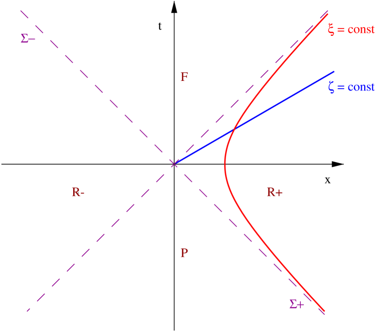
Figure 1: Rindler partition of Minkowski spacetime. The hyperbolic trajectory is given by $\xi=constant$.

We can use the Rindler-Fulling expansion of the field based on the solutions of the Klein-Gordon equation in the Rindler wedge [4, 13]

$$u_{\nu\mathbf{k}}(x)=\frac{\sqrt{\sinh{\pi\nu}}}{2\pi^{2}}e^{-i\nu\zeta+i\mathbf{k}\mathbf{y}}K_{i\nu}(k\xi)\equiv u_{\nu\mathbf{k}}(\xi,\mathbf{y})e^{-i\nu\zeta}$$ (16)

and recalculate the Green function for $x,x^{\prime}$ in the Rindler wedge. Now we must treat Minkowski vacuum as a many-particle state of Rindler quanta, therefore the Wightman function is replaced [4] by

$$D^{+}[x,x^{\prime}]=\int_{0}^{\infty}\!d\nu\!\int\!d^{2}\mathbf{k}\!\left\{u_{\nu\mathbf{k}}(x)u^{*}_{\nu\mathbf{k}}(x^{\prime})\left[1+n_{\nu\mathbf{k}}\right]+u^{*}_{\nu\mathbf{k}}(x)u_{\nu\mathbf{k}}(x^{\prime})\,n_{\nu\mathbf{k}}\right\},$$ (17)

where the mean number of Rindler quanta in Minkowski vacuum is given by a thermal distribution at the Unruh-Davies temperature $T_{a}=a/2{\pi}$

$$n_{\nu\mathbf{k}}=\frac{1}{e^{2\pi\nu}-1}.$$ (18)

For the response function on the hyperbolic trajectory, we then get [13, 4, 7]

$$\frac{\mathcal{F}(E)}{T} = \int^{\infty}_{-\infty}d\sigma e^{iE\sigma}\int_{0}^{\infty}d\nu\int d^{2}\mathbf{k}\mid u_{\nu\mathbf{k}}(1/a,\mathbf{0})\mid^{2}\times$$ (19)

$$\left\{e^{-i\nu a\sigma}\;\left[\frac{1}{e^{2\pi\nu}-1}\right]+e^{i\nu a\sigma}\;\left[1+\frac{1}{e^{2\pi\nu}-1}\right]\right\}.$$

After integration we obtain the following expression for the probability of emission per unit proper time of a Minkowski particle with defined transverse momentum to be compared with (13)

$$\frac{d\,\mathcal{P}(E)}{Td^{2}\mathbf{k}}\Big{|}_{Mink,Emiss} = \left|\langle\mathcal{E}|m(0)|0\rangle\right|^{2}\;\frac{2\pi}{a}\mid u_{|E|/a,\mathbf{k}}(1/a,\mathbf{0})\mid^{2}\times$$ (20)

$$\left\{\Theta(E)\;\left[\frac{1}{e^{2\pi E/a}-1}\right]+\Theta(-E)\;\left[1+\frac{1}{e^{2\pi|E|/a}-1}\right]\right\}.$$

In terms of elementary processes of absorption and emission of Rindler quanta, this can be written as [6, 7, 14]

$$\frac{d\,\mathcal{P}(E)}{Td^{2}\mathbf{k}}\Big{|}_{Mink,Emiss} = \Theta(E)\;\left[\frac{1}{e^{2\pi E/a}-1}\right]\frac{d\,\mathcal{P}(E)}{Td^{2}\mathbf{k}}\Big{|}_{Rind,Abs}+$$ (21)

$$\Theta(-E)\;\left[1+\frac{1}{e^{2\pi|E|/a}-1}\right]\frac{d\,\mathcal{P}(E)}{Td^{2}\mathbf{k}}\Big{|}_{Rind,Emiss}.$$

This gives the relation between the two observers description of the “click” of the detector. The emission of a Minkowski particle with defined transverse momentum with a shift $E$ of the detector level corresponds to the induced absorption of a Rindler quantum from the bath when the detector goes up or to the spontaneous plus induced emission of a Rindler scalar photon to the bath when the detector goes down (see fig.2 for diagrammatic description of the situation).

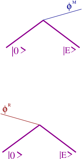
Figure 2: The emission of a Minkowski quantum $\phi^{M}$ with the excitation of the detector corresponds to the induced absorption of a Rindler quantum $\phi^{R}$ from the FDU thermal bath.

The equality between equations (13) and (20) can be checked out by the explicit use of Nicholson’s integral with imaginary order and argument of the Bessel functions [15]).

3 Classical radiation and the inert limit

The connection with the radiation of a classical source is made by following DeWitt’s [11] observation that if the detector were inert, possessing no internal degrees of freedom, the pattern of particle emission would be that of a given accelerating source. Taking the limit $E\rightarrow 0$ no structure is left to the detector. In the inertial expression (13), the limit is done by setting $E=0$, identifying $\left|\langle 0|m(0)|0\rangle\right|^{2}$ with the classical monopole squared charge $q^{2}$ and evaluating the two integrals [16]

$$\frac{d\,\mathcal{P}(0)}{Td^{2}\mathbf{k}}\Big{|}_{Mink,Emiss}=q^{2}\int^{\infty}_{-\infty}d\eta\int^{\infty}_{-\infty}\frac{d\sigma}{16\pi^{3}a}e^{-2i\frac{k}{a}\sinh{\frac{\sigma}{2}}\,\cosh{\eta}}=\frac{q^{2}}{4\pi^{3}a}\,K^{2}_{0}(k/a).$$ (22)

For the non-inertial computation there are two competing contributions, the probability of absorption/emission of a Rindler quantum that goes to zero and the termal factor that goes to infinity. Nevertheless the limit is well defined and gives the same finite result as above. That is for $E\rightarrow 0^{+}$

$$\left|\langle E|m(0)|0\rangle\right|^{2}\;\frac{2\pi}{a}\frac{\sinh{\pi E/a}}{4\pi^{4}}\mid K_{iE/a}(k\xi)\mid^{2}\;\frac{1}{e^{2\pi E/a}-1}\quad\longrightarrow\quad\frac{q^{2}}{4\pi^{3}a}\,K^{2}_{0}(k/a).$$ (23)

Here we also make connection with the result of Ref.[8, 9, 10] with the advantage of getting the correct numerical factor (In [8, 9, 10] an aditional $\sqrt{2}$ has to be put by hand..

The same result is obtained for $E\rightarrow 0^{-}$ and therefore our computation regardless of the initial state of the detector. We stress that the equivalence in the inert limit is preserved due to the special role played by the zero-energy Rindler scalar photons of the bath which are the ones involved in this limit.

The previous calculations can be generalized to more than two transverse dimensions. For D-2 transverse dimensions the response function in the inert limit gives

$$\frac{F(0)}{T}=\frac{(2\pi^{2})^{1-D}}{\Gamma(\frac{D-1}{2})}\Gamma(\frac{D}{2}-1)^{2}.$$ (24)

This remains finite, regardless the parity of the number of space-time dimensions ($D>2$). One concludes that the underlying statistics is of the Bose-Einstein type because a growing number of quanta in the $E\rightarrow 0$ states is needed in order to have a finite induced effect. This confirms the arguments of Ref. [17, 7] in the sense that there is no inversion of the statistics in odd dimensions as proposed in the literature.

4 Conclusion

The point we want to stress in this work is that for an accelerated Unruh-DeWitt detector the calculations based on emission/absorption of Rindler quanta in the presence of the Fulling-Davis-Unruh bath are shown to be equivalent to the standard ones involving Minkowski quanta. We emphasize that the behavior of the Unruh-DeWitt detector in the limit of zero energy gap corresponds to that of a classical source linearly coupled to the quantum field. In this form we make contact with a previous approach [6, 7, 8, 9, 10] where the classical radiation pattern was obtained in semiclassical formalism through and regularization procedure.

In addition, the finite response per unit proper time in the inert limit in any $D>2$ spacetime dimensions confirms that the underlying statistics is of the Bose-Einstein kind, because the overpopulation of the zero-energy states is necessary in order to wind up with a finite induced emission probability.

Acknowledgment

We thank Víctor Villalba and Nami Fux Svaiter for useful discussions.

References

- [1] R.Peierls, Surprises in theoretical physics. (Princeton University Press, Princeton, 1979).
- [2] D.G.Boulware, Ann. Phys. (N.Y.) 124,169 (1980).
- [3] S.A.Fulling, Phys. Rev. D 7,2850 (1973).
- [4] N.D.Birrell and P.C.W.Davies, Quantum field theory in curved space. (Cambridge University Press, Cambridge, 1982).
- [5] W.Rindler, Essential Relativity. (Springer-Verlag, Berlin/New York, 1977).
- [6] W.G.Unruh and R.M.Wald, Phys. Rev. D 29,1047 (1984).
- [7] V.L.Ginzburg and V.P.Frolov, Sov. Phys. Usp 30,1073 (1987).
- [8] A.Higuchi, G.E.A.Matsas, and D.Sudarsky, Phys. Rev. D 45,R3308 (1992).
- [9] A.Higuchi, G.E.A.Matsas, and D.Sudarsky, Phys. Rev. D 46,3450 (1992).
- [10] H.Ren and E.J.Weinberg, Phys. Rev. D 49,6526 (1994).
- [11] B.S.DeWitt, in General Relativity: An Einstein Centennary Survey, edited by S.W.Hawking and W.Israel (Cambridge University Press, Cambridge, England, 1979).
- [12] H.Kolbenstvedt, Phys. Rev. D 38,1118 (1988).
- [13] D.W.Sciama, P.Candelas, and D.Deutsch, Adv. Phys. 30,327 (1981).
- [14] B.F.Svaiter and N.F.Svaiter, Phys. Rev. D 46,5267 (1992).
- [15] G.N.Watson, A treatise on the theory of Bessel functions. (Cambridge, 1966), p. 444.
- [16] I.S.Gradshteyn and I.M.Ryzhik, Tables of integrals, series and products. (Academic, New York, 1980).
- [17] W.G.Unruh, Phys. Rev. D 34,1222 (1986).