Impulsive waves in the Nariai universe

Abstract

A new class of exact solutions is presented which describes impulsive waves propagating in the Nariai universe. It is constructed using a six-dimensional embedding formalism adapted to the background. Due to the topology of the latter, the wave front consists of two non-expanding spheres. Special sub-classes representing pure gravitational waves (generated by null particles with an arbitrary multipole structure) or shells of null dust are analyzed in detail. Smooth isometries of the metrics are briefly discussed. Furthermore, it is shown that the considered solutions are impulsive members of a more general family of radiative Kundt spacetimes of type-$II$. A straightforward generalization to impulsive waves in the anti-Nariai and Bertotti–Robinson backgrounds is described. For a vanishing cosmological constant and electromagnetic field, results for well known impulsive pp -waves are recovered.

I Introduction

Many exact solutions of Einstein’s equations are known which describe radiative spacetimes (a recent review and references are provided, e.g., in Bičák (2000)). As special cases, impulsive waves have been widely investigated. Their geometry is characterized by the Dirac delta contribution to the curvature tensor, supported on a null hypersurface, which is interpreted as an impulsive field propagating in a given background. In the simplest situation this is a constant-curvature space (Minkowski, de Sitter or anti-de Sitter) and all main features of such metrics are well known (see Podolský (2002) and references therein). In particular, these belong to two distinct families in which the waves are either expanding or non-expanding, thus being understood as limiting cases of sandwich waves of the Robinson–Trautman or the Kundt classes, respectively. Specific non-expanding solutions were originally obtained by applying the Aichelburg–Sexl ultra-relativistic boost Aichelburg and Sexl (1971) to different elements of the Kerr–Newman and Weyl families (see, e.g., Ferrari and Pendenza (1989); Loustó and Sánchez (1992); Hotta and Tanaka (1993); Balasin and Nachbagauer (1995); Podolský and Griffiths (1998a)). It has then been shown Griffiths and Podolský (1997); Podolský and Griffiths (1998b) that the whole class of non-expanding impulsive pure gravitational waves (with the only exception of plane waves) is generated by null particles with an arbitrary multipole structure, corresponding to singularities of the metric tensor. Moreover, as an extension of the Penrose’s geometrical method Penrose (1972), Dray and ’t Hooft have introduced a “shift-function” technique, which enables to construct non-expanding impulsive waves also in non-constant-curvature backgrounds. They used it to derive the field produced by a massless particle Dray and ’t Hooft (1985a) or by a spherical shell of null matter Dray and ’t Hooft (1985b) located at the horizon of a Schwarzschild black hole. Their approach has been later generalized Sfetsos (1995) to include a cosmological constant $\Lambda$ and matter fields.

Now, a simple observation is that non-expanding impulsive waves propagating in all possible spherically symmetric vacuum backgrounds with $\Lambda=0$ have thus been explicitly described. This is guaranteed by the celebrated Birkhoff theorem (see, e.g., Kramer et al. (1980)), which leaves the Schwarzschild metric (with the Minkowski universe as a trivial sub-case) as the only possibility. However, the generalized version of this theorem admitting a non-vanishing $\Lambda$ Foyster and McIntosh (1972); Barnes (1973); Kramer et al. (1980) provides a richer class of non-equivalent metrics. Namely, one has not only the Schwarzschild–(anti-)de Sitter solutions, but also the Nariai metric Nariai (1951), when $\Lambda>0$ (its $\Lambda<0$ counterpart, to which we shall refer as “anti-Nariai”, admits different symmetries).

The Nariai line-element, which actually (in a Euclidean notation) dates back to Kasner Kasner (1925), is indeed a non-singular solution of the vacuum Einstein’s equations with a positive cosmological constant, $R_{\mu\nu}=\Lambda g_{\mu\nu}$. It is the direct product of a two-dimensional de Sitter space with a 2-sphere. It admits a 6-parameters group of motions and is not conformally flat. Therefore, it is both locally and globally distinguished from the de Sitter space. Besides the historical attention it deserved thanks to its geometrical properties Kasner (1925); Nariai (1951); Bertotti (1959); Kramer et al. (1980), more recently it has been the object of a renewed interest, since it emerges as the extremal limit of Schwarzschild–de Sitter black holes Ginsparg and Perry (1983); Bousso and Hawking (1996); Caldarelli et al. (2001) (which is not equivalent to consider “extreme” black holes, studied, e.g., in Podolský (1999)). Thus, it can be viewed as a “degenerate” black hole, in which the two horizons have the same (maximum) size and are in thermal equilibrium at the temperature $T=\sqrt{\Lambda}/2\pi$. Admitting a regular Euclidean section, it turns out to be a good “instanton” for the study of quantum pair creation of black holes during inflation. In more general terms, a “charged” version of the Nariai metric Bertotti (1959) (see also Elizalde and Hildebrandt (2001)) is interpreted as a degenerate Reissner–Nordström–de Sitter black hole Hawking and Ross (1995). This has been considered also in dilatonic theories, e.g. in Bousso (1997).

To our knowledge, impulsive waves in the Nariai universe have not yet explicitly been studied. It is the purpose of the present paper to construct and analyze non-expanding impulsive waves propagating in this background, thus filling a “gap” in the classification of impulsive waves in spherically symmetric spaces.

Sec. II reviews the Nariai geometry, useful in the sequel. The complete metric representing impulsive waves is presented in Sec. III. This is done by means of a global six-dimensional formalism adapted to the Nariai spacetime. The unusual geometry of the wave front is described by means of six- and global natural four-coordinates. In Sec. IV contributions to the curvature due to the waves are calculated, and a general exact solution to the vacuum field equations is provided. It is shown that the only possible regular solution is given by a trivial “gauge” term, which can be removed by an appropriate coordinate transformation. Then, the unavoidable singularities are interpreted as point sources of pure gravitational waves. Also, a complementary situation is discussed in which there is no impulse in the Weyl scalars and the gravitational field is entirely due to shells of null matter. Sec. V deals with smooth symmetries of the impulsive metrics. In Sec. VI it is shown that these non-expanding impulsive waves are in fact a limiting case of a more general type-$II$ spacetime of the Kundt class, as a “profile” function approaches the Dirac delta. It is thus suggested to interpret this general spacetime as the Nariai universe with gravitational radiation. A straightforward generalization to impulsive waves in other direct product backgrounds, in particular the Bertotti–Robinson universe, is sketched in Sec. VII.

II The Nariai spacetime

The Nariai universe Nariai (1951); Kasner (1925) can be conveniently visualized as a 4-submanifold of a six-dimensional Lorentzian flat manifold

$${\rm d}s^{2}=-{\rm d}{Z_{0}}^{2}+{\rm d}{Z_{1}}^{2}+{\rm d}{Z_{2}}^{2}+{\rm d}{Z_{3}}^{2}+{\rm d}{Z_{4}}^{2}+{\rm d}{Z_{5}}^{2},$$ (1)

determined by two constraints

$$-{Z_{0}}^{2}+{Z_{1}}^{2}+{Z_{2}}^{2}=a^{2},\qquad{Z_{3}}^{2}+{Z_{4}}^{2}+{Z_{5}}^{2}=a^{2},$$ (2)

where $a>0$ is related to the cosmological constant by

$$\Lambda=\frac{1}{a^{2}}.$$ (3)

It is then obvious that the spacetime is the direct product dS${}_{2}\times{\mathbb{S}}^{2}$ of two constant curvature 2-spaces, thus being “symmetric” (i.e., $R_{\mu\nu\rho\sigma;\tau}=0$) Kramer et al. (1980), and admits a six-dimensional group of isometries $SO(2,1)\times SO(3)$. In particular, it is spherically symmetric (but not isotropic) and (locally) static. Furthermore, the group acts transitively (i.e., the spacetime is homogeneous) and has a two-dimensional isotropy subgroup at each point, composed of one boost and one spatial rotation. Note that the charged Nariai solution Bertotti (1959) is obtained by replacing the second constraint in (2) with ${Z_{3}}^{2}+{Z_{4}}^{2}+{Z_{5}}^{2}=b^{2}$ (where $b=\mbox{constant}\neq a$), provided $a^{-2}+b^{-2}=2\Lambda$.

Various four-dimensional parametrizations of (1) with (2) are known. The static Schwarzschild-like one (covering only a part of the whole manifold)

$${\rm d}s^{2}= - \left(1-\frac{r^{2}}{a^{2}}\right){\rm d}t^{2}+\left(1-\frac{r^{2}}{a^{2}}\right)^{-1}{\rm d}r^{2}$$ (4)

$$+ a^{2}({\rm d}\theta^{2}+\sin^{2}\theta{\rm d}\phi^{2}),$$

is given by (for $0<r<a$)

$$Z_{0} = \sqrt{a^{2}-r^{2}}\sinh(t/a),\quad Z_{1}=\sqrt{a^{2}-r^{2}}\cosh(t/a),$$

$$Z_{2} = r,\qquad Z_{3}=a\sin\theta\cos\phi,$$ (5)

$$Z_{4} = a\sin\theta\sin\phi,\qquad Z_{5}=a\cos\theta.$$

With the natural re-definition

$$Z_{0} = a\sinh(\tau/a),$$

$$Z_{1} = a\cosh(\tau/a)\cos\chi,$$ (6)

$$Z_{2} = a\cosh(\tau/a)\sin\chi,$$

for $\tau\in(-\infty,+\infty)$ and $\chi\in[0,2\pi]$ periodic, one gets the global Kantowski–Sachs cosmological line-element

$${\rm d}s^{2}=-{\rm d}\tau^{2}+a^{2}\cosh^{2}(\tau/a){\rm d}\chi^{2}+a^{2}({\rm d}\theta^{2}+\sin^{2}\theta{\rm d}\phi^{2}),$$ (7)

in which the ${\mathbb{R}}\times{\mathbb{S}}^{1}\times{\mathbb{S}}^{2}$ topology is manifest. Note that while the ${\mathbb{S}}^{1}$ factor describes a circle which shrinks to a minimum radius $a$ at $\tau=0$ and then re-expands, the ${\mathbb{S}}^{2}$ has a constant radius $a$ at any time (this is different from the well known behaviour of the de Sitter universe, whose ${\mathbb{S}}^{3}$ spatial section contracts and expands isotropically). Now, for constant $\theta$ and $\phi$, it is straightforward to visualize the conformal structure of the spacetime by defining a conformal time

$$\eta=2\arctan(e^{\tau/a})\in[0,\pi].$$ (8)

The diagram (Fig. 1) is that of a two-dimensional de Sitter space, with a spacelike infinity for timelike and null lines.

Figure 1: The conformal diagram of the non-singular Nariai universe in coordinates $(\eta,\chi)$ of (7) and (8). The spacelike boundaries $\eta=0$ and $\eta=\pi$ correspond to $\tau=-\infty$ and $\tau=+\infty$, respectively. The angular coordinate $\chi$ spans a circle, so that $\chi=0$ and $\chi=2\pi$ are identified. Each point of this representation is a 2-sphere in the actual spacetime. Solid and dashed null lines represent the (disconnected) past and future event horizon, respectively, for a geodesic observer $\chi=0$.

Obviously, each point of the diagram corresponds to a two-sphere of constant radius $a$, parametrized by $(\theta,\phi)$. For the geodesic observer $\chi=0$, for instance, both the future and past event horizon consist of two connected components. These are given for the former by $\eta_{+}^{f}=\chi-\pi$ and $\eta_{-}^{f}=\pi-\chi$, and for the latter by $\eta_{+}^{p}=\chi$ and $\eta_{-}^{p}=2\pi-\chi$.

In order to express the curvature tensor, we introduce another suitable coordinate system. First, we define six-dimensional null coordinates $U=\frac{1}{\sqrt{2}}(Z_{0}+Z_{1})$ and $V=\frac{1}{\sqrt{2}}(Z_{0}-Z_{1})$, and then

$$U=\frac{u}{\Omega},\qquad V=-\frac{v}{\Omega},\qquad Z_{2}=\frac{1-\Lambda uv}{\sqrt{2\Lambda}\Omega},$$

$$Z_{3}=\frac{\zeta+\bar{\zeta}}{\sqrt{2}\Sigma},\quad Z_{4}=-i\frac{\zeta-\bar{\zeta}}{\sqrt{2}\Sigma},\quad Z_{5}=\frac{2-\Sigma}{\sqrt{\Lambda}\Sigma},$$ (9)

with

$$\Omega={\textstyle\frac{1}{\sqrt{2}}}(1+\Lambda uv),\qquad\Sigma=1+{\textstyle\frac{1}{2}}\Lambda\zeta\bar{\zeta}.$$ (10)

This gives a Kruskal form

$${\rm d}s^{2}=\frac{4{\rm d}u{\rm d}v}{(1+\Lambda uv)^{2}}+\frac{2{\rm d}\zeta{\rm d}\bar{\zeta}}{(1+\frac{1}{2}\Lambda\zeta\bar{\zeta})^{2}},$$ (11)

in which the limit $\Lambda\rightarrow 0$ can be explicitly performed, leading to the Minkowski spacetime. Using the natural null tetrad $\mbox{\boldmath$k$}=\Omega\,\partial_{v}$, $\mbox{\boldmath$l$}=-\Omega\,\partial_{u}$, $\mbox{\boldmath$m$}=\Sigma\partial_{\bar{\zeta}}$, the only non-trivial curvature components are

$$\Psi_{2}=-\frac{\Lambda}{3},\qquad R=4\Lambda.$$ (12)

This explicitly demonstrates that the Nariai spacetime is a Petrov type-$D$ solution of vacuum Einstein’s equations with a positive cosmological constant.

III Geometry of impulsive waves

It is known that non-expanding impulsive waves in the (anti-)de Sitter backgrounds can be conveniently described as five-dimensional impulsive pp -waves plus an appropriate constraint Hotta and Tanaka (1993); Podolský and Griffiths (1998b). In close analogy, we introduce here a class of impulsive waves propagating in the Nariai universe as a six-dimensional pp -wave constrained by (2), i.e. as a metric

$${\rm d}s^{2}= - 2{\rm d}U{\rm d}V+{\rm d}{Z_{2}}^{2}+{\rm d}{Z_{3}}^{2}+{\rm d}{Z_{4}}^{2}+{\rm d}{Z_{5}}^{2}$$ (13)

$$+ \tilde{H}(Z_{2},Z_{3},Z_{4},Z_{5})\,\delta(U)\,{\rm d}U^{2},$$

with

$$-2UV+{Z_{2}}^{2}=a^{2},\qquad{Z_{3}}^{2}+{Z_{4}}^{2}+{Z_{5}}^{2}=a^{2},$$ (14)

where $\delta(U)$ is the Dirac distribution. For $U\neq 0$ the spacetime (13) (with (14)) obviously reduces to the Nariai background. The impulse is located on the null 3-manifold $U=0=Z_{0}+Z_{1}$, given by

$$Z_{2}=\pm a,\qquad{Z_{3}}^{2}+{Z_{4}}^{2}+{Z_{5}}^{2}=a^{2}.$$ (15)

This is the history of two non-intersecting and non-expanding 2-spheres of constant area $4\pi a^{2}$, so that the spatial sections of the 3-wave front are disconnected 2-manifolds (see Fig. 2).

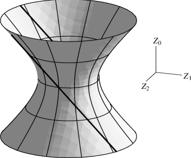
Figure 2: The 2-hyperboloid visualizes the dS₂ factor of the Nariai spacetime dS${}_{2}\times{\mathbb{S}}^{2}$, once that the coordinates $Z_{3}$, $Z_{4}$ and $Z_{5}$ have been suppressed (see (1) and (2)). Then, each point corresponds to a 2-sphere of a constant area $4\pi a^{2}$ in the four-dimensional spacetime. The parallel straight lines $Z_{0}+Z_{1}=0$ are the histories of two of these spheres, which propagate at the speed of light and represent the impulse (15).

In the global coordinates of (7), which display the ${\mathbb{S}}^{1}\times{\mathbb{S}}^{2}$ spatial sections of the universe, the impulsive wave stays at $\cos\chi=-\tanh(\tau/a)$, with its connected components at

$$\chi_{+} = \arccos[-\tanh(\tau/a)],$$

$$\chi_{-} = 2\pi-\arccos[-\tanh(\tau/a)],$$ (16)

respectively. These are nothing but the components $\eta_{\pm}^{p}$ of the past event horizon of the geodesic observer $\chi=0$ in the Nariai cosmos, see Sec. II and Fig. 1. Formula (III) demonstrates that the two ${\mathbb{S}}^{2}$-components propagate in opposite directions along the circle ${\mathbb{S}}^{1}$, from $\chi_{+}=0$, $\chi_{-}=2\pi$ as $\tau\rightarrow-\infty$, to $\chi_{+}=\pi/2$, $\chi_{-}=3\pi/2$ at $\tau=0$ and $\chi_{\pm}=\pi$ as $\tau\rightarrow+\infty$. Thus, the history of each of them spans exactly one-half of the ${\mathbb{S}}^{1}$. Note that, although their $\chi$-separation decreases (as $\tau\rightarrow\pm\infty$), they never collide. Indeed, the ${\mathbb{S}}^{1}$ contracts and then re-expands in such a way that the spatial separation between these, $\Delta l=a\cosh(\tau/a)[(\chi_{-}-\chi_{+})\mod{2\pi}]$, is always finite. In particular, this reaches its maximum value $\pi a$ at $\tau=0$, when the circle contracts to a minimum radius $a$, and approaches $2a$ in the limit $\tau\rightarrow\pm\infty$, when the circle expands indefinitely. In order to visualize the propagation of the impulsive wave, let us suppress one spatial dimension by fixing $\theta=\theta_{0}=\mbox{constant}\neq 0,\,\pi$ in (7). Then, each connected component of the wave front reduces to a circle of a constant radius $a\sin\theta_{0}$, spanned by $\phi$, which propagates on a flat 2-torus ${\mathbb{S}}^{1}\times{\mathbb{S}}^{1}$, with coordinates $(\chi,\phi)$. This is represented in Fig. 3 (which is not completely faithful, as a flat 2-torus can not be isometrically immersed in ${\mathbb{R}}^{3}$).

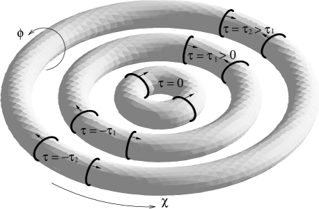
Figure 3: Suppressing the $\theta$ in global coordinates (7), each spatial section of the Nariai universe reduces to a 2-torus parametrized by $(\chi,\phi)$, as drawn for different values of the proper time $\tau$. The torus is contracting for $\tau<0$, reaches its minimum size at $\tau=0$, and then re-expands indefinitely as $\tau\rightarrow+\infty$. However, such an expansion is anisotropic, only involving the angular coordinate $\chi$. At any time, the impulsive wave front consists of two non-expanding 2-spheres, represented here by circles of constant radius. These propagate in opposite directions from one side of the universe ($\chi=0$) to the other ($\chi=\pi$), as $\tau$ grows from $-\infty$ to $+\infty$.

It is interesting to compare the description of the present geometry and its global structure with that of non-expanding waves in a de Sitter spacetime, given in Podolský and Griffiths (1997).

IV Curvature and Einstein’s equations

In this section we evaluate the curvature tensor and solve the vacuum equations associated with the impulsive waves presented in Sec. III. With the parametrization (II) (and a trivial re-scaling $H\equiv\sqrt{2}\tilde{H}$) the metric (13) with (14) becomes

$${\rm d}s^{2}=\frac{H(\zeta,\bar{\zeta})\delta(u){\rm d}u^{2}+4{\rm d}u{\rm d}v}{(1+\Lambda uv)^{2}}+\frac{2{\rm d}\zeta{\rm d}\bar{\zeta}}{(1+\frac{1}{2}\Lambda\zeta\bar{\zeta})^{2}}.$$ (17)

Note that (17) could equivalently be obtained by means of the Dray–’t Hooft shift-function method Dray and ’t Hooft (1985a); Sfetsos (1995) applied to (11), or by using the general construction based on the generalized Kerr–Schild class Balasin (2000). Now, we employ the null tetrads formalism. We replace $l$ in the null tetrad of Sec. II with the more general $\mbox{\boldmath$l$}=\Omega\left(-\partial_{u}+\frac{1}{4}H\delta(u)\partial_{v}\right)$, and consider the distributional identity $u\delta(u)=0$. Expressions (12) remain unchanged and the only new curvature components are

$$\Psi_{4} = -{\textstyle\frac{1}{4}}\Sigma\left(\Lambda\bar{\zeta}H_{\zeta}+\Sigma H_{\zeta\zeta}\right)\delta(u),$$

$$\Phi_{22} = -{\textstyle\frac{1}{4}}\Sigma^{2}H_{\zeta\bar{\zeta}}\,\delta(u).$$ (18)

Thus, in general the metric (17) describes impulsive gravitational waves plus an impulse of null matter localized at $u=0$. Correspondingly, on the wavefront the spacetime is of Petrov type-$II$, with energy-momentum representing pure radiation ($4\pi\,T_{\mu\nu}=\Phi_{22}\,k_{\mu}k_{\nu}$). The impulsive contribution to the Weyl tensor is of type-$N$ (as expected from the general theory of lightlike shells Barrabès and Israel (1991), see also Barrabès et al. (1997); Barrabès and Hogan (1998)). The limit $\Lambda\rightarrow 0$ in (17) and (18) leads to results for well known impulsive pp -waves.

Pure gravitational waves occur when the simple vacuum field equation $H_{\zeta\bar{\zeta}}=0$ is satisfied, i.e. for

$$H(\zeta,\bar{\zeta})=f(\zeta)+\bar{f}(\bar{\zeta}),$$ (19)

in which $f(\zeta)$ is an arbitrary analytic function of $\zeta$. This is again formally analogous to well known pp -waves Kramer et al. (1980); Griffiths and Podolský (1997), except that the coordinates $(\zeta,\bar{\zeta})$ span 2-spheres, here, instead of 2-planes. In particular, for $H=a_{0}=\mbox{constant}$ the line-element (17) represents only the Nariai background in different coordinates, since the impulse is removable by the discontinuous coordinate transformation

$$u^{\prime}=\frac{u}{1-{\textstyle\frac{1}{4}}a_{0}\Lambda u{\Theta}(u)},\qquad v^{\prime}=v+{\textstyle\frac{1}{4}}a_{0}{\Theta}(u),\qquad\zeta^{\prime}=\zeta,$$ (20)

where ${\Theta}(u)$ is the step function. This result is in full agreement with the Birkhoff theorem, as a metric (17) with a constant $H$ clearly represents a spherically symmetric vacuum spacetime.

General non-trivial solutions (19) necessarily contain singularities localized on the wavefront, which can be considered as null point sources of impulsive gravitational waves. In order to achieve such a physical interpretation, it is convenient to follow Podolský and Griffiths (1998b) in introducing a coordinate

$$z=\cos\theta,$$ (21)

so that $Z_{3}=a\sqrt{1-z^{2}}\cos{\phi}$, $Z_{4}=a\sqrt{1-z^{2}}\sin{\phi}$, $Z_{5}=az$. This parametrization enables us to rewrite the matter content of the spacetime as

$$\Phi_{22}=-{\textstyle\frac{1}{8}}{\bf\Delta}H\,\delta(u),$$ (22)

where ${\bf\Delta}\equiv\Lambda\{\partial_{z}[(1-z^{2})\partial_{z}]+(1-z^{2})^{-1}\partial_{\phi}\partial_{\phi}\}$ is the Laplacian on a 2-sphere. By the standard method, one can now solve the vacuum equation $\Phi_{22}=0$ separating $H(z,\phi)={\cal Z}(z)\Phi(\phi)$. To each angular mode $\Phi_{m}=\cos[m(\phi-\phi_{m})]$ (with $m=0,1,2,\ldots$ and $\phi_{m}$ being arbitrary “phase” constants) corresponds an associated Legendre equation $\{\partial_{z}[(1-z^{2})\partial_{z}]-m^{2}/(1-z^{2})\}{\cal Z}_{m}=0$ (with missing $l(l+1)$-term). For each value of $m$, this has the general solutions

$${\cal Z}_{0}(z)=a_{0}+\frac{b_{0}}{2}\ln\frac{1+z}{1-z},$$

$${\cal Z}_{m}(z)=b_{m}F_{m}(z)+b_{-m}F_{-m}(z)\quad(m\geq 1),$$ (23)

where $a_{0}$, $b_{0}$ and $b_{\pm m}$ are “amplitude” constants and $F_{\pm m}(z)$ are defined by the recurrence formula

$$F_{\pm m}(z)\equiv(1-z^{2})^{m/2}\frac{{\rm d}^{m}}{{\rm d}z^{m}}\ln(1\mp z)^{1/2}.$$ (24)

These functions, which are basically positive and negative powers of $[(1+z)/(1-z)]^{1/2}=\cot(\theta/2)$, are singular at $z=\pm 1$, respectively. The general vacuum solution is then given by a superposition

$$H(z,\phi)=a_{0}+\frac{b_{0}}{2}\ln\frac{1+z}{1-z}$$

$${}+\sum_{m=1}^{\infty}[b_{m}F_{m}(z)+b_{-m}F_{-m}(z)]\cos[m(\phi-\phi_{m})].\qquad$$ (25)

Recalling that $a_{0}$ represents a removable term, it is now clear that non-trivial solutions (25) contain at least one singularity at $z=1$ or $z=-1$, i.e. at one of the poles $\theta=0,\,\pi$ of the “twin” spherical wave surfaces. By defining the source term as $J(z,\phi)\equiv-a^{2}{\bf\Delta}H(z,\phi)$, one finds $J(z,\phi)=b_{0}J_{0}(z)+\sum_{m=1}^{\infty}[b_{m}J_{m}(z,\phi)+b_{-m}J_{-m}(z,\phi)]$. The $m$-components are given by

$$J_{0}(z)=\delta(1-z)-\delta(1+z),$$

$$J_{\pm m}(z,\phi)=-(1-z^{2})^{m/2}\delta^{(m)}(1\mp z)\cos[m(\phi-\phi_{m})],$$ (26)

where $\delta^{(m)}$ is the $m$-derivative of $\delta$. Calculations which justify (26) follow the approach of Podolský and Griffiths (1998b) and are summarized in Appendix A. According to (26), for $m\neq 0$ each $J_{\pm m}$ term in the energy-momentum tensor describes a single point source with an $m$-pole structure. For $m=0$, instead, there is a pair of “monopole” particles (compare with Griffiths and Podolský (1997); Podolský and Griffiths (1998b)). Thus, the general solution (25) contains null particles at the poles of both twin 2-spheres which compose the wave front. However, $\Phi_{22}$ is linear in $H$ and the background is invariant under rotations. Hence, in general, one can superimpose any number of such arbitrary multipole particles arbitrarily located over the impulsive surfaces. Note that the monopole term in $b_{0}$ describes an axially symmetric spacetime. This is the counterpart of the Aichelburg–Sexl Aichelburg and Sexl (1971) and Hotta–Tanaka Hotta and Tanaka (1993) solutions for impulsive waves in constant curvature spaces. A comment on the energy conditions satisfied by these sources is given in Appendix B.

It is finally natural to investigate the complementary situation in which there is no gravitational impulse in the Weyl scalars. Again using the coordinates $(z,\phi)$ on the wave front, the complex equation $\Psi_{4}=0$ splits into its real and imaginary parts

$$(1-z^{2})^{2}H_{zz}-H_{\phi\phi}=0,\qquad(1-z^{2})H_{z\phi}+zH_{\phi}=0.$$ (27)

After separation of variables, these have the general solution (up to a removable constant term)

$$H(z,\phi)=b_{0}z+b_{1}\sqrt{1-z^{2}}\cos(\phi-\phi_{1}).$$ (28)

In this case, the gravitational field is entirely generated by two spherical shells of null matter which form the impulse. In particular, no point particles (singularities) appear. Again, $b_{0}$ is the coefficient of an axially symmetric term.

Except for the “pure” solutions (25) and (28), the spacetime (17) in general describes impulsive waves generated by an arbitrary superposition of multipole point-like sources and an impulse of null dust in the Nariai universe.

V Symmetries of the impulsive solutions

In Podolský and Ortaggio (2001) (smooth) symmetries of non-expanding impulsive waves in (anti-)de Sitter spacetime have been investigated using an embedding formalism similar to that of (13) and (14). In particular, it has been demonstrated that these are the transformations which leave both the four-background and the embedding space (a five-dimensional pp -wave) unchanged.

An analogous analysis can be performed in the present case. Again, smooth symmetries of the full spacetime must also be symmetries of the background (described in Sec. II). Among these, it is natural to consider the isometries of the embedding space (13) (see Aichelburg and Balasin (1996)). Then, it turns out that spacetimes representing non-expanding impulsive waves in the Nariai universe in general admit at least one Killing vector field. Namely, for an arbitrary $\tilde{H}$ the metric (13) and the constraints (14) are invariant under the null rotation generated by

$$Z_{2}\,\partial_{V}+U\,\partial_{Z_{2}},$$ (29)

i.e. under the transformation ($\tilde{\beta}$ being a parameter)

$$U^{\prime} =U,\qquad V^{\prime}=V+\tilde{\beta}\,Z_{2}+{\textstyle\frac{1}{2}}\tilde{\beta}^{2}\,U,$$ (30)

$$Z_{2}^{\prime} =Z_{2}+\tilde{\beta}\,U,\qquad Z_{i}^{\prime}=Z_{i}\quad(i=3,4,5).$$

In terms of the four-coordinates of (17), this corresponds to the generator

$$\partial_{v}+\Lambda u^{2}\partial_{u},$$ (31)

with the finite transformation

$$u^{\prime}=\frac{u}{1-\beta\Lambda u},\qquad v^{\prime}=v+\beta,\qquad\zeta^{\prime}=\zeta.$$ (32)

In the limit $\Lambda\rightarrow 0$, this simply becomes the translation of pp -waves, generated by $\partial_{v}$. Particular choices of $\tilde{H}$ may represent spacetimes with more isometries. For instance, in the case $\tilde{H}=\tilde{H}(Z_{5})$ one has an axially symmetric metric independent of $\phi$, with the further Killing vector $Z_{3}\partial_{Z_{4}}-Z_{4}\partial_{Z_{3}}$ (see Sec. IV for two explicit examples). From the Killing equations it can be easily verified that, in the axially symmetric case, no more symmetries are permitted (except for a trivial $\tilde{H}$). A richer structure is in principle expected if one allows for non-smooth transformations, for specific shapes of the profile function $\tilde{H}$. However, we do not deal with this issue here, as it involves mathematical subtleties which go beyond the scope of this paper (see Aichelburg and Balasin (1997) for such a study in the case of impulsive pp -waves).

VI The limit of exact sandwich waves

In this section we wish to demonstrate that non-expanding impulsive waves in the Nariai spacetime constructed above can be naturally understood as limiting cases of more general exact radiative spacetimes. Within the wide Kundt class of non-diverging solutions Kramer et al. (1980), let us concentrate here on the sub-family

$${\rm d}s^{2}={\rm d}u^{2}\left(\Lambda w^{2}+2H\right)-2{\rm d}u{\rm d}w+\frac{2{\rm d}\zeta{\rm d}\bar{\zeta}}{(1+\frac{1}{2}\Lambda\zeta\bar{\zeta})^{2}},$$ (33)

in which $H=H(u,\zeta,\bar{\zeta})$ is analytic in $(\zeta,\bar{\zeta})$ and has an arbitrary dependence on $u$. With the standard null tetrad $\mbox{\boldmath$k$}=\partial_{w}$, $\mbox{\boldmath$l$}=\partial_{u}+\frac{1}{2}(\Lambda w^{2}+2H)\partial_{w}$, $\mbox{\boldmath$m$}=\Sigma\partial_{\bar{\zeta}}$, the curvature components read

$$\Psi_{2} = -\frac{\Lambda}{3},\qquad\Psi_{4}=-\Sigma\left(\Lambda\bar{\zeta}H_{\zeta}+\Sigma H_{\zeta\zeta}\right),$$

$$\Phi_{22} = -\Sigma^{2}H_{\zeta\bar{\zeta}},\qquad R=4\Lambda.$$ (34)

Thus, in general the spacetime is of type-$II$. The vacuum equation $\Phi_{22}=0$ clearly has the solution

$$H(u,\zeta,\bar{\zeta})=f(u,\zeta)+\bar{f}(u,\bar{\zeta}),$$ (35)

see the discussion in Sec. IV. In this case, the metric (33) represents the Kundt vacuum spacetime with a positive cosmological constant. In particular, for $H=0$ this turns out to be the Nariai universe (11), as the substitution

$$w=-\frac{\sqrt{2}}{\Omega}v$$ (36)

explicitly shows.

Now, we can understand the null coordinate $u$ in (33) as playing the role of a “retarded time” and the function $H$ that of a “wave profile”. Then, if $H$ is taken to be non-vanishing only for a finite range of $u$, it is natural to interpret the metric (33) with (35) as describing a pure gravitational field of finite duration which propagate in a Nariai background (with the speed of light). Moreover, using (36) it is easy to verify that in the limit of “instantaneous” waves, $H(u,\zeta,\bar{\zeta})\rightarrow H(\zeta,\bar{\zeta})\delta(u)$, spacetimes (33) are exactly the previously considered non-expanding impulsive waves (17). This is a strict analogy with non-expanding impulsive waves in constant curvature backgrounds, which are known to be impulsive members of the Kundt class of type-$N$ solutions of vacuum Einstein’s equations (see Podolský (1998)). In general, one can construct sandwich gravitational waves with an arbitrary profile, e.g. shock or smooth waves. In any case, these waves are spherical but non-expanding.

In view of these results, we suggest to interpret the exact solutions (33) (with (35)) as describing a Nariai universe containing gravitational radiation.

VII Impulsive waves in other direct product backgrounds

The construction of Sec. III can be easily generalized to describe non-expanding impulsive waves propagating in other well known spacetimes which are the direct product of two 2-spaces with non-vanishing constant curvature. Namely, we can replace (13) and (14) with the more general metric

$${\rm d}s^{2}= - 2{\rm d}U{\rm d}V+\epsilon_{1}{\rm d}{Z_{2}}^{2}+{\rm d}{Z_{3}}^{2}+{\rm d}{Z_{4}}^{2}+\epsilon_{2}{\rm d}{Z_{5}}^{2}$$ (37)

$$+ \tilde{H}(Z_{2},Z_{3},Z_{4},Z_{5})\,\delta(U)\,{\rm d}U^{2},$$

$$-2UV+\epsilon_{1}{Z_{2}}^{2}=\epsilon_{1}a^{2},\quad{Z_{3}}^{2}+{Z_{4}}^{2}+\epsilon_{2}{Z_{5}}^{2}=\epsilon_{2}a^{2},$$ (38)

in which $\epsilon_{1},\,\epsilon_{2}=\pm 1$ give the sign of the curvature of each 2-space. A four-parametrization which generalizes (II) and (17) reads

$${\rm d}s^{2}=\frac{H(\zeta,\bar{\zeta})\delta(u){\rm d}u^{2}+4{\rm d}u{\rm d}v}{(1+\epsilon_{1}a^{-2}uv)^{2}}+\frac{2{\rm d}\zeta{\rm d}\bar{\zeta}}{(1+\frac{1}{2}\epsilon_{2}a^{-2}\zeta\bar{\zeta})^{2}}.$$ (39)

We are thus left with four possible different non-trivial spacetimes, according to the signs of $\epsilon_{1}$ and $\epsilon_{2}$. Note that backgrounds with $\epsilon_{1}=-1$ contain closed timelike curves, unless one takes a universal covering. The case $\epsilon_{1}=\epsilon_{2}=+1$ corresponds to the impulsive solution in the Nariai background described in previous sections (with $\Lambda=a^{-2}$). When $\epsilon_{1}=\epsilon_{2}=-1$, one has waves in the anti-Nariai spacetime AdS${}_{2}\times{\mathbb{H}}^{\,2}$. This is a vacuum solution with $\Lambda=-a^{-2}<0$, which appears, for example, in the extremal limit of topological black holes Caldarelli et al. (2001) (in which case ${\mathbb{H}}^{\,2}$ is compactified to a Riemann surface of genus $g>1$). The famous Bertotti–Robinson metric AdS${}_{2}\times{\mathbb{S}}^{2}$ Bertotti (1959); Robinson (1959) is recovered when $\epsilon_{1}=-\epsilon_{2}=-1$, and describes a conformally flat spacetime filled with a uniform electromagnetic field. The last possibility, $\epsilon_{1}=-\epsilon_{2}=1$, gives a conformally flat “unphysical” spacetime dS${}_{2}\times{\mathbb{H}}^{\,2}$ with negative energy density. Combined situations ($\Lambda$ plus an electromagnetic field) may also occur by applying the prescription suggested in Sec. II for the charged Nariai solution, see Bertotti (1959). In any case, metrics (39) in general describe a superposition of impulsive gravitational waves (with point-like sources) and impulsive null dust, the geometry of the wave front being ${\mathbb{S}}^{2}$ (for $\epsilon_{2}=+1$) or ${\mathbb{H}}^{\,2}$ (for $\epsilon_{2}=-1$). The essential conformal structure depends only on the first factor in the direct product metric, which contains $\epsilon_{1}$. For the dS₂ is shown in Fig. 1. For the AdS₂, one similarly obtains that of Fig. 4, which resembles the case of impulsive waves in a full anti-de Sitter spacetime Podolský and Griffiths (1997).

Figure 4: The conformal diagram of the Bertotti–Robinson and anti-Nariai spacetimes with non-expanding impulsive waves, given by the two null lines. Each point represents a two-dimensional (pseudo-)sphere. The timelike boundaries $R=0$ and $R=\pi$ correspond to null and spacelike infinity on opposite sides of the universe. As long as the coordinate time $t$ is assumed to be periodic, $t=0$ and $t=2\pi$ have to be identified. Otherwise, one can unwrap $t$ and build an endless tower of these conformal diagrams, from $t=-\infty$ to $t=+\infty$.

Note that in the limit $a^{2}\rightarrow\infty$ (that is, when the cosmological constant and the electromagnetic field approach zero) all the metrics (39) become impulsive pp -waves.

The analysis of Secs. IV, V and VI can be straightforwardly adapted to any of the above possible backgrounds.

VIII Concluding remarks

A new class of exact solution of Einstein’s equations with a positive cosmological constant has been presented. This describes impulsive gravitational and/or matter waves propagating in a Nariai universe, and thus completes the classification of non-expanding impulsive waves in spherically symmetric vacuum spacetimes. A convenient six-dimensional embedding formalism has been employed for the construction. The formal structure of the solutions has been shown to be similar to that of previously known non-expanding impulsive waves in (anti-)de Sitter spacetimes Hotta and Tanaka (1993); Podolský and Griffiths (1998b). Nevertheless, the background is now non-trivial and displays different topological properties. The geometrical approach has also been used for discussion of symmetries of these solution (following Podolský and Ortaggio (2001)) and for constructing impulsive waves in other direct product backgrounds, such as the anti-Nariai and the Bertotti–Robinson universe.

Vacuum field equations have been solved in full generality, and singularities of the solutions have been interpreted in terms of point multipole sources of gravitational waves. Our analysis followed the works by Griffiths and Podolský for solutions in Minkowski Griffiths and Podolský (1997) and (anti-)de Sitter Podolský and Griffiths (1998b) backgrounds. But there is a difference. In the solutions Griffiths and Podolský (1997); Podolský and Griffiths (1998b), the axially symmetric monopole terms are physically understood as fields generated by ultra-relativistic particles, initially obtained by an appropriate boosting technique by Aichelburg and Sexl Aichelburg and Sexl (1971) and Hotta and Tanaka Hotta and Tanaka (1993). A generalization by Podolský and Griffiths themselves Podolský and Griffiths (1998a) extends such an interpretation to higher multipole terms (at least when $\Lambda=0$). However, it seems that no exact static solutions are known in an asymptotically Nariai spacetime. Therefore, so far we can not relate the above null solutions to any such field boosted to the speed of light.

Finally, we have observed that (similarly as in the case of constant curvature spacetimes Podolský (1998)) these impulsive solutions in the Nariai universe belong to a more general family of Kundt spacetimes. This family can thus be interpreted as representing exact sandwich gravitational waves of finite duration, or even the full Nariai cosmos filled with gravitational radiation. It seems to us that these solutions did not appear previously, at least in explicit form. Very similar metrics have been already considered, see, e.g., equations (27.54) and (31.37) in Kramer et al. (1980) (for special choices of the arbitrary functions/parameters therein). However, these describe non-vacuum type-$N$ spacetimes. According to considerations in Secs. IV and VII, they can be interpreted as a Bertotti–Robinson universe with gravitational radiation.

Appendix A

By a slight modification of the derivation by Podolský and Griffiths Podolský and Griffiths (1998b) for the case of impulsive waves in (anti-) de Sitter spacetimes, we present here basic relations leading to formulae (26). One starts by expanding the function $\ln(1-z)^{1/2}$ for $z\in(-1,1)$ in terms of the complete system of Legendre polynomials as (see, e.g., Hansen (1975))

$$\ln(1-z)^{1/2}={\textstyle\frac{1}{2}}(\ln 2-1)-\sum_{l=1}^{\infty}\frac{l+\frac{1}{2}}{l(l+1)}P_{l}(z).$$ (40)

Since $P_{l}(-z)=(-1)^{l}P_{l}(z)$, it also holds

$$\frac{1}{2}\ln\frac{1+z}{1-z}=\sum_{l=1}^{\infty}\frac{l+\frac{1}{2}}{l(l+1)}P_{l}(z)[1-(-1)^{l}].$$ (41)

For higher $m$-terms, combing the definition (24) for $F_{m}(z)$ with (40) and the recurrence formula for the associated Legendre functions of the first kind,

$$P_{l}^{m}(z)=(-1)^{m}(1-z^{2})^{m/2}\frac{{\rm d}^{m}}{{\rm d}z^{m}}P_{l}(z),$$ (42)

one gets

$$F_{m}(z)=-(-1)^{m}\sum_{l=1}^{\infty}\frac{l+\frac{1}{2}}{l(l+1)}P_{l}^{m}(z).$$ (43)

Recalling that $\int_{-1}^{1}{\rm d}zP_{l}(z)P_{j}(z)=(l+1/2)^{-1}\delta_{lj}$ and $P_{l}(1)=1$, one can write the distributional expansion

$$\delta(1-z)=\sum_{l=0}^{\infty}{\textstyle\left(l+\frac{1}{2}\right)}P_{l}(z).$$ (44)

If now the operator ${\bf L_{m}}\equiv\partial_{z}[(1-z^{2})\partial_{z}]-m^{2}(1-z^{2})^{-1}$ is introduced (for $m\geq 0$), the identity ${\bf L_{m}}P_{l}^{m}(z)=-l(l+1)P_{l}^{m}(z)$ follows, since $P_{l}^{m}(z)$ are solutions of an associated Legendre equation. Applying such an identity to (41) and (43) and making use of (42) and (44), one gets

$${\bf L_{0}}\frac{1}{2}\ln\frac{1+z}{1-z}=\delta(1+z)-\delta(1-z),$$

$${\bf L_{m}}F_{m}(z)=(1-z^{2})^{m/2}\delta^{(m)}(1-z),$$ (45)

where $\delta^{(m)}(1-z)\equiv{\rm d}^{m}\delta(1-z)/{\rm d}z^{m}$. An analogous proof can be carried out for $F_{-m}(z)$.

Appendix B

The (distributional) energy conditions obeyed by the idealized point sources (26) of Sec. IV are here discussed. First of all, for pure radiation matter ($T_{\mu\nu}\sim k_{\mu}k_{\nu}$) the weak, strong and dominant energy conditions turn out to be completely equivalent, due to the null character of $k$. Then, it suffices to concentrate on the weak condition. Given a non-spacelike vector $t$ and considering the results of Sec. IV, that reads

$$T_{\mu\nu}t^{\mu}t^{\nu}=(32\pi)^{-1}\Lambda\,J(z,\phi)\,\delta(u)(\mbox{\boldmath$k$}\cdot\mbox{\boldmath$t$})^{2}\geq 0.$$ (46)

Clearly, this is automatically satisfied everywhere but at $u=0$, where the possible matter is localized (from now on, we also disregard the trivial case $\delta(u)(\mbox{\boldmath$k$}\cdot\mbox{\boldmath$t$})^{2}=0$). On the wave front, the crucial sign is given by $J(z,\phi)$, since $\delta(u)$ is a non-negative distribution. Now, the multipoles with odd $m$ in (26) have to be considered only as formal, since contain terms (such as $x^{m/2}\delta^{(m)}(x)$) which are not defined as distributions within Schwartz’s theory. These will not be discussed here. The even-multipoles, instead, are described by distributions with a non-definite “sign”, thus violating (46). This agrees with physical intuition as, roughly speaking, a multipole must contain “charge” densities of both signs. As expected, it turns out that the surface integral of such $J_{\pm m}$ is indeed vanishing (thus the total energy is non-negative). On the other hand, the monopole $J_{0}$ in (26) is described by the difference of two distributions with a well-defined sign. Then, it should be interpreted as representing two particles with equal and opposite energy densities. Note that the “unphysical” negative energy density is in this case mathematically unavoidable, and can geometrically be understood by considering the equivalent electrostatic problem of a point charge on a sphere (the electric lines of force generated by a source at the South pole must re-converge on a sink at the North pole, instead of spreading out at infinity, as in the planar case).

We conclude showing that, anyway, combined solutions (with point particles and null dust) exist which do not violate the energy conditions. We may simply adapt a “heuristic argument” by Balasin and Nachbagauer Balasin and Nachbagauer (1995) (who also indicate how to make the proof rigorous). Thanks to the generalized Kerr–Schild form of the metric (17) (see Footnote 3), the squared norm of $t$ can be decomposed as

$$\mbox{\boldmath$t$}\cdot\mbox{\boldmath$t$}={\textstyle\frac{1}{2}}H\delta(u)(\mbox{\boldmath$k$}\cdot\mbox{\boldmath$t$})^{2}+\tilde{\mbox{\boldmath$g$}}(\mbox{\boldmath$t$},\mbox{\boldmath$t$})\leq 0.$$ (47)

In this, it is the first “infinite” term that determines $t$ being causal. Therefore, if we consider a profile function $H$ which is strictly positive on the whole wave front ($z\in[-1,1]$), (47) can never hold there. In this case, (46) does not have to be satisfied, thus not restricting $J(z,\phi)$. For instance, the positive function $H(z)=e^{z}-\ln(1-z^{2})^{1/2}$ is associated with the source term $J(z)=e^{z}(z^{2}+2z-1)+\delta(1-z)+\delta(1+z)-1$.

References

- Bičák (2000) J. Bičák, in Einstein’s Field Equations and Their Physical Implications, edited by B. G. Schmidt (Springer-Verlag, Berlin, 2000), vol. 540 of Lect. Notes Phys., pp. 1–126.
- Grosser et al. (2001) M. Grosser, M. Kunzinger, M. Oberguggenberger, and R. Steinbauer, Geometric Theory of Generalized Functions with Applications to General Relativity, vol. 537 of Mathematics and its Applications (Kluwer Academic Publishers, Dordrecht, 2001).
- Podolský (2002) J. Podolský, in Gravitation: Following the Prague Inspiration, edited by O. Semerák, J. Podolský, and M. Žofka (World Scientific, Singapore, 2002), pp. 205–246, to appear, eprint gr-qc/0201029.
- Aichelburg and Sexl (1971) P. C. Aichelburg and R. U. Sexl, Gen. Rel. Grav. 2, 303 (1971).
- Ferrari and Pendenza (1989) V. Ferrari and P. Pendenza, Gen. Rel. Grav. 22, 1105 (1989).
- Loustó and Sánchez (1992) C. O. Loustó and N. Sánchez, Nucl. Phys. B 383, 377 (1992).
- Hotta and Tanaka (1993) M. Hotta and M. Tanaka, Class. Quantum Grav. 10, 307 (1993).
- Balasin and Nachbagauer (1995) H. Balasin and H. Nachbagauer, Class. Quantum Grav. 12, 707 (1995).
- Podolský and Griffiths (1998a) J. Podolský and J. B. Griffiths, Phys. Rev. D 58, 124024 (1998a).
- Griffiths and Podolský (1997) J. B. Griffiths and J. Podolský, Phys. Lett. A 236, 8 (1997).
- Podolský and Griffiths (1998b) J. Podolský and J. B. Griffiths, Class. Quantum Grav. 15, 453 (1998b).
- Penrose (1972) R. Penrose, in General Relativity: papers in honour of J. L. Synge, edited by L. O’Raifeartaigh (Clarendon Press, Oxford, 1972), pp. 101–115.
- Dray and ’t Hooft (1985a) T. Dray and G. ’t Hooft, Nucl. Phys. B 253, 173 (1985a).
- Dray and ’t Hooft (1985b) T. Dray and G. ’t Hooft, Commun. Math. Phys. 99, 613 (1985b).
- Sfetsos (1995) K. Sfetsos, Nucl. Phys. B 436, 721 (1995).
- Kramer et al. (1980) D. Kramer, H. Stephani, M. MacCallum, and E. Herlt, Exact Solutions of Einstein’s Field Equations (Cambridge University Press, Cambridge, 1980).
- Foyster and McIntosh (1972) J. M. Foyster and C. B. G. McIntosh, Commun. Math. Phys. 27, 241 (1972).
- Barnes (1973) A. Barnes, Commun. Math. Phys. 33, 75 (1973).
- Nariai (1951) H. Nariai, Sci. Rep. Tohoku Univ. 35, 62 (1951).
- Kasner (1925) E. Kasner, Trans. Am. Math. Soc. 27, 101 (1925).
- Bertotti (1959) B. Bertotti, Phys. Rev. 116, 1331 (1959).
- Ginsparg and Perry (1983) P. Ginsparg and M. J. Perry, Nucl. Phys. B 222, 245 (1983).
- Bousso and Hawking (1996) R. Bousso and S. W. Hawking, Phys. Rev. D 54, 6312 (1996).
- Caldarelli et al. (2001) M. Caldarelli, L. Vanzo, and S. Zerbini, in Geometrical Aspects of Quantum Fields: Proceedings of the 2000 Londrina Workshop, edited by A. A. Bytsenko, A. E. Gonçalves, and B. M. Pimentel (World Scientific, Singapore, 2001), pp. 56–63.
- Podolský (1999) J. Podolský, Gen. Rel. Grav. 31, 1703 (1999).
- Elizalde and Hildebrandt (2001) E. Elizalde and S. R. Hildebrandt (2001), eprint gr-qc/0103064.
- Hawking and Ross (1995) S. W. Hawking and S. F. Ross, Phys. Rev. D 52, 5865 (1995).
- Bousso (1997) R. Bousso, Phys. Rev. D 55, 3614 (1997).
- Balasin (2000) H. Balasin, Class. Quantum Grav. 17, 1913 (2000).
- Podolský and Griffiths (1997) J. Podolský and J. B. Griffiths, Phys. Rev. D 56, 4756 (1997).
- Barrabès and Israel (1991) C. Barrabès and W. Israel, Phys. Rev. D 43, 1129 (1991).
- Barrabès et al. (1997) C. Barrabès, G. F. Bressange, and P. A. Hogan, Phys. Rev. D 55, 3477 (1997).
- Barrabès and Hogan (1998) C. Barrabès and P. A. Hogan, Phys. Rev. D 58, 044013 (1998).
- Podolský and Ortaggio (2001) J. Podolský and M. Ortaggio, Class. Quantum Grav. 18, 2689 (2001).
- Aichelburg and Balasin (1996) P. C. Aichelburg and H. Balasin, Class. Quantum Grav. 13, 723 (1996).
- Aichelburg and Balasin (1997) P. C. Aichelburg and H. Balasin, Class. Quantum Grav. 14, A31 (1997).
- Podolský (1998) J. Podolský, Class. Quantum Grav. 15, 3229 (1998).
- Robinson (1959) I. Robinson, Bull. Acad. Polon. 7, 351 (1959).
- Hansen (1975) E. R. Hansen, A Table of Series and Products (Prentice-Hall, Inc., Englewood Cliffs, N J, 1975).