Magnetic Brane-worlds

Abstract

We investigate brane-worlds with a pure magnetic field and a perfect fluid. We extend earlier work to brane-worlds, and find new properties of the Bianchi type I brane-world. We find new asymptotic behaviours on approach to the singularity and classify the critical points of the dynamical phase space. It is known that the Einstein equations for the magnetic Bianchi type I models are in general oscillatory and are believed to be chaotic, but in the brane-world model this chaotic behaviour does not seem to be possible.

1 Introduction

Developments in string theory have inspired the construction of brane-worlds, in which standard-model gauge fields are confined to our three-dimensional brane-world, while gravity propagates in all the spatial dimensions. A simple five-dimensional class of such models allows for a non-compact extra dimension via a novel mechanism for localization of gravity around the brane at low energies[1, 2]. This mechanism is the warping of the metric by a negative five-dimensional cosmological constant. These models have been generalized to admit cosmological branes [3], and they provide an interesting arena in which to impose cosmological tests on extra-dimensional generalizations of Einstein’s theory. One of the unusual features of this structure is that brane-worlds can feel the effects of non-local anisotropic stresses in the bulk dimensions. These graviton stresses are unconstrained by dynamical equations specified on the brane but for a wide range of behaviours they completely determine the evolution of small anisotropies on the brane-world and can slow the their decay to such an extent that their effects are directly detectable today in the temperature anisotropy of the microwave background radiation[4]. The evolution of anisotropic brane-worlds has been studied recently by several authors [5, 6, 7, 8, 9, 10]. They consider only the behaviour of simple anisotropies in universes with perfect fluid matter sources. However, it is known that the evolution of simple anisotropic universes with isotropic three-curvature is very sensitive to the presence of trace-free matter sources with anisotropic pressures, [11, 12, 13]. Such stresses are inevitable in anisotropic cosmologies at early times because of the presence of collisionless gravitons, collisionless asymptotically-free particles, and electric or magnetic fields. These stresses also mimic the effects of more general anisotropic curvature anisotropies in more general anisotropic universe (because the latter can be viewed as an effective stress of long-wavelength gravitational waves). Small anisotropic pressures serve to slow the decay of the shear anisotropy to a logarithm of the time during the radiation era and to a slow power law during the dust era. These anisotropic stresses can arise because of intrinsic anisotropic stresses on the brane or via the induced graviton stresses from the bulk. In this paper we are going to consider the detailed behaviour of the simplest example: a pure magnetic field on a flat anisotropic brane with Bianchi type I geometry. Whereas the study of ref. [4] was interested in the late-time behaviour we shall be interested primarily in the behaviour as $t\rightarrow 0.$

The possibility of isotropization and homogenisation of cosmological models have been an important study since the original equations for gravitational interaction where put down in 1915 by Einstein. The general relativistic anisotropic models called the Bianchi models have been studied in great detail both in general relativistic cosmologies [14, 11, 15] and to some extent in the brane-world scenario . A feature that has been known to exist in the Bianchi models are oscillatory solutions[16, 17], and even chaotic solutions [18, 19, 20, 21, 22, 23]. The chaotic behaviour in the general relativistic vacuum Bianchi type VIII and IX models has been well studied, and chaotic behaviour for the general relativistic Bianchi type I model with a magnetic field has been conjectured [16] and studied for the case of form fields [24]. There are many similarities between magnetic Bianchi universes and the behaviour of pre-big-bang string cosmologies [25]. For further discussion of magnetic field effects in general cosmological models see also refs. [26, 27].

In the brane-worlds model the dynamics change because of the influence of terms varying as the square of the isotropic and anisotropic pressure as $t\rightarrow 0$. We investigate the Bianchi type I brane-world with a perfect fluid and a pure magnetic field in the context of a possible chaotic behaviour. This extends the general relativistic study by LeBlanc [16] to the brane-world scenario. We will show that unlike the general relativity case, chaotic behaviour is probably completely absent for all perfect fluids as a result of the non-linear stresses.

This paper is organized as follows: First we put down the fundamental equations of motion. We use the representation of LeBlanc to facilitate comparisons, and introduce expansion-normalized variables. Since we are primarily interested in the initial singularity, we find some approximate solutions near the initial singularity for different magnetic configurations. All of these approximate solutions correspond to equilibrium points for the full set of equations, and so we provide a stability analysis of the equilibrium points found.

2 Equations of motion for a Bianchi type I brane-world

The Bianchi cosmological models can be classified according to the commutation relations of their invariant 1-forms, $\omega^{i}$. We will use an orthonormal frame of vector fields $\{e_{\mu}\}$, and align the frame so that $e_{0}=\partial_{t}$, the fluid vector field. This implies that the spatial triad $\{e_{a}\}$ spans the tangent space at each point of the group orbits. Using the commutation relations for this vector basis, the commutator functions $C_{~{}\beta\gamma}^{\alpha}(t)$ are given by

$$[e_{\alpha},e_{\beta}]=C_{~{}\alpha\beta}^{\gamma}(t)e_{\gamma}$$ (1)

In the Bianchi Class A case we have the relations

$$C_{~{}0b}^{a}(t)=-\Theta_{~{}b}^{a}(t)-\epsilon_{~{}bc}^{a}\Omega^{c}(t),~{}C_{~{}bc}^{a}=\epsilon_{bcd}n^{ad}$$ (2)

The $\Theta_{~{}b}^{a}(t)$ are the frame components of the volume expansion tensor of the fluid, or the extrinsic curvature. The vector $\Omega^{c}(t)$ is the angular velocity of the spatial triad with respect to a set of Fermi-propagated axes. The extrinsic curvature $\Theta_{\mu\nu}$ is separated into its trace, $\Theta$, the volume expansion, and its trace-free part $\sigma_{\mu\nu},$ the shear:

$$\Theta_{\mu\nu}=\frac{1}{3}\Theta h_{\mu\nu}+\sigma_{\mu\nu}$$ (3)

We will also assume that we have a non-zero electromagnetic (EM) field and a non-interacting perfect fluid. The perfect-fluid energy momentum tensor is

$$T_{\mu\nu}^{PF}=(\rho+p)u_{\mu}u_{\nu}+pg_{\mu\nu}$$ (4)

Further, we will assume a barotropic equation of state for the fluid for the pressure $p$ and density $\rho$:

$$p=(\gamma-1)\rho$$ (5)

where $\gamma\in[0,2]$ is constant. The perfect fluid solves the usual conservation equation

$$\dot{\rho}+\gamma\Theta\rho=0$$ (6)

The energy-momentum tensor of the EM field can be expressed as

$$T_{\mu\nu}^{EM}=\rho_{EM}u_{\mu}u_{\nu}+p_{EM}h_{\mu\nu}+\pi_{\mu\nu},$$ (7)

where $\rho_{EM}$ and $p_{EM}$ are the energy density and the isotropic pressure, respectively, and the tensor $h_{\mu\nu}=g_{\mu\nu}+u_{\mu}u_{\nu}$ projects orthogonal to the $u^{\mu}$ on the brane, and $\pi_{\mu\nu}$ is the tracefree anisotropic pressure tensor. In the case of an electric field $E$ and magnetic field $B$ the energy-momentum tensor can be written in general as

$$T_{\mu\nu}^{EM}=-\frac{1}{4}F^{\alpha\beta}F_{\alpha\beta}g_{\mu\nu}+F_{\mu\alpha}F_{\nu}^{~{}\alpha}$$ (8)

where the anisotropic stress is

$$\pi_{\mu\nu}=-E_{\mu}E_{\nu}-B_{\mu}B_{\nu}+\frac{1}{3}(E^{2}+B^{2})h_{\mu\nu}$$ (9)

and the pressure and density are given by

$$\rho_{EM}=3p_{EM}=\frac{1}{2}(E^{2}+B^{2})$$ (10)

Demanding that the perfect fluid and the EM field be separately conserved requires eqn. (6)

$$\dot{\rho}_{EM}+\Theta(\rho_{EM}+p_{EM})+\sigma^{\mu\nu}\pi_{\mu\nu}=0.$$ (11)

For a Bianchi type I model the commutator between the vectors of the spatial triad all commute so

$$C_{~{}bc}^{a}=0$$ (12)

This allows us to have a pure magnetic field[28]. This is not the case for all Bianchi models. We shall therefore specialise to the case of a Bianchi type I model with a vanishing electric field.

We now consider the evolution equations on the brane [29, 30] for the expansion scale factor, shear, and energy densities. The latter consist of the perfect fluid density, the magnetic energy and the dark energy term $\mathcal{U}$. The non-local energy conservation equation for the dark energy $\mathcal{U}$ is

$$\dot{\mathcal{U}}+\frac{4}{3}\Theta\mathcal{U}+\sigma^{\mu\nu}\mathcal{P}_{\mu\nu}=$$

$$\frac{\kappa^{4}}{12}\left[3\pi^{\mu\nu}\dot{\pi}_{\mu\nu}+3(\rho+p)\sigma^{\mu\nu}\pi_{\mu\nu}+\Theta\pi^{\mu\nu}\pi_{\mu\nu}-\sigma^{\mu\nu}\pi_{\alpha\mu}\pi_{\nu}^{~{}\alpha}\right]$$ (13)

where the overdot means $u^{\mu}\nabla_{\mu}\equiv d/dt$, $\mathcal{P}_{\mu\nu}$ is the unconstrained bulk graviton stress, and $\kappa^{2}\equiv 8\pi G$. The constraint equation is

$$H^{2}=\frac{\Lambda}{3}+\frac{1}{6}\sigma^{\mu\nu}\sigma_{\mu\nu}-\frac{1}{6}\mathcal{R}+\frac{\kappa^{2}}{3}\left[\rho\left(1+\frac{\rho}{2\lambda}\right)-\frac{3}{4\lambda}\pi_{\mu\nu}\pi^{\mu\nu}\right]+\frac{2\mathcal{U}}{\kappa^{2}\lambda}$$ (14)

where $\mathcal{R}$ is the 3-curvature of the brane, $\lambda$ is the brane tension, $\Lambda$ the cosmological constant, and $H=\frac{1}{3}\Theta$ is the Hubble expansion parameter. The Gauss-Codazzi shear propagation equations are:

$$\dot{\sigma}_{<\mu\nu>}+\Theta\sigma_{\mu\nu}=\kappa^{2}\pi_{\mu\nu}+\frac{\kappa^{2}}{2\lambda}\left[-(\rho+3p)\pi_{\mu\nu}+\pi_{\alpha<\mu}\pi_{~{}\nu>}^{\alpha}\right]+\frac{6}{\kappa^{2}\lambda}\mathcal{P}_{\mu\nu}-\mathcal{R}_{<\mu\nu>}$$ (15)

where $A_{<\mu\nu>}$ for a tensor $A_{\mu\nu}$, means the projected, symmetric and trace-free part [29, 30]. The volume expansion propagation is governed by Raychaudhuri’s equation

$$\dot{\Theta}+\frac{1}{3}\Theta^{2}+\sigma^{\mu\nu}\sigma_{\mu\nu}+\frac{1}{2}\kappa^{2}(\rho+3p)-\Lambda=$$

$$-\frac{1}{2\lambda\kappa^{2}}\left[\kappa^{4}(2\rho^{2}+3\rho p)+12\mathcal{U}\right]$$ (16)

Here, for simplicity we shall assume that $\mathcal{P}_{\mu\nu}=0$ in order for the equations to close and we set $\mathcal{R}_{<\mu\nu>}=0$ in the Bianchi I universe and also assume $\Lambda=0$. The dark energy, $\mathcal{U}$ (which can in principle be of either sign) on the other hand cannot be set to zero in the presence of a non-zero anisotropic stress. In addition to these equations the magnetic field satisfies Maxwell’s equations:

$$\dot{B}_{\mu}=-\frac{2}{3}\Theta B_{\mu}+\sigma_{\mu\nu}B^{\nu}$$ (17)

Since we shall be concerned with the early time behaviour we can ask if there is an initial singularity. In the brane-world we can write the energy-momentum tensor as a sum of the classical energy-momentum tensor and a term that come from brane-effects only. A sufficient condition for a singularity is that the classical energy-momentum tensor obeys the strong energy condition (SEC), and that $\mathcal{U}>0$. We must however emphasize that we can still have a singularity even if this condition is violated.

The equations in the orthonormal frame reduce to the following first-order system:

$$\dot{\Theta} = \partial_{t}\Theta$$ (18)

$$\dot{B}_{a} = \partial_{t}B_{a}-\epsilon_{abc}\Omega^{c}B^{b}$$ (19)

$$\dot{\sigma}_{ab} = \partial_{t}\sigma_{ab}+2\sigma_{(a}^{d}\epsilon_{b)cd}\Omega^{c}$$ (20)

$$\dot{\pi}_{ab} = \partial_{t}\pi_{ab}+2\pi_{(a}^{d}\epsilon_{b)cd}\Omega^{c}$$ (21)

We still have an unused gauge freedom to choose the orientation of the spatial triad. We choose the orientation so that the magnetic field is aligned with $e_{1}$, thus ensuring $B_{2}=B_{3}=0$ while $B_{1}=h$. From the Maxwell equations for $B_{a}$ this yields the constraints

$$\Omega^{2}=-\sigma_{13},~{}\Omega^{3}=\sigma_{12}$$ (22)

The $\Omega^{1}$ is still left undetermined, but to simplify the equations we will choose a frame so that $\Omega^{1}=0$. This choice of gauge makes the anisotropic-stress tensor diagonal (as in the general case of refs.[11], [13]), with

$$\pi_{\mu\nu}=D_{\mu\nu}h^{2}$$ (23)

where $D_{\mu\nu}=$ $diag(0,-\frac{2}{3},\frac{1}{3},\frac{1}{3})$.

Introducing the parameters $\sigma_{\pm}$, defined by

$$(\sigma_{11},\sigma_{22},\sigma_{33})=(-2\sigma_{+},\sigma_{+}+\sqrt{3}\sigma_{-},\sigma_{+}-\sqrt{3}\sigma_{-}),$$

allows the full set of equations to be written as a first-order dynamical system:

$$\partial_{t}h = -\frac{2}{3}\Theta h-2\sigma_{+}h$$ (24)

$$\partial_{t}\rho = -\gamma\Theta\rho$$ (25)

$$\partial_{t}\Theta = -\frac{1}{3}\Theta^{2}\ -\sigma^{2}-\frac{1}{2}[(3\gamma-2)\rho+h^{2}]$$ (26)

$$-\frac{\chi}{8}[4(3\gamma-1)\rho^{2}+(6\gamma+4)\rho h^{2}+3h^{4}]-6\chi\mathcal{U}$$

$$\partial_{t}\mathcal{U} = -\frac{4}{3}\Theta\mathcal{U}-\frac{h^{2}}{6}\left[\Theta h^{2}+\frac{5}{3}\sigma_{+}h^{2}-3\gamma\sigma_{+}\rho\right]$$ (27)

$$\partial_{t}\sigma_{+} = -\Theta\sigma_{+}-\sigma_{12}^{2}-\sigma_{13}^{2}+\frac{1}{3}h^{2}\left(1-\frac{\chi}{2}\left[(3\gamma-2)\rho+\frac{4}{3}h^{2}\right]\right)$$ (28)

$$\partial_{t}\sigma_{-} = -\Theta\sigma_{-}-\frac{1}{\sqrt{3}}(\sigma_{12}^{2}-\sigma_{13}^{2})$$ (29)

$$\partial_{t}\sigma_{23} = -\Theta\sigma_{23}-2\sigma_{12}\sigma_{13}$$ (30)

$$\partial_{t}\sigma_{12} = -\Theta\sigma_{12}+(3\sigma_{+}+\sqrt{3}\sigma_{-})\sigma_{12}+\sigma_{13}\sigma_{23}$$ (31)

$$\partial_{t}\sigma_{13} = -\Theta\sigma_{13}+(3\sigma_{+}-\sqrt{3}\sigma_{-})\sigma_{13}+\sigma_{12}\sigma_{23},$$ (32)

where $\chi=(\kappa^{2}\lambda)^{-1}$ is constant and where we have set $\kappa=1$ implicitly by making the redefinitions: $\kappa h\longrightarrow h$ and $\kappa^{2}\rho\longrightarrow\rho$. Interestingly, there is a further symmetry in these equations. By a change of variables

$$\sigma_{12}+i\sigma_{13} = \sigma_{A}e^{i\phi}$$ (33)

$$\sqrt{3}\sigma_{-}+i\sigma_{23} = (\sigma_{B}+i\sigma_{C})e^{2i\phi},$$ (34)

the equation for $\phi$ turns into

$$\partial_{t}\phi=\sigma_{C}$$ (35)

and can be completely eliminated from the system. Thus, this variable can be ignored. The remaining equations for the shear are

$$\partial_{t}\sigma_{+} = -\Theta\sigma_{+}-\sigma_{A}^{2}+\frac{1}{3}h^{2}\left(1-\frac{\chi}{2}\left[(3\gamma-2)\rho+\frac{4}{3}h^{2}\right]\right)$$ (36)

$$\partial_{t}\sigma_{A} = (-\Theta+3\sigma_{+}+\sigma_{B})\sigma_{A}$$ (37)

$$\partial_{t}\sigma_{B} = -\Theta\sigma_{B}-\sigma_{A}^{2}+2\sigma_{C}^{2}$$ (38)

$$\partial_{t}\sigma_{C} = (-\Theta-2\sigma_{B})\sigma_{C}$$ (39)

A further simplification is achieved by defining a new set of expansion normalized variables:

$$\Sigma_{+} = \frac{3\sigma_{+}}{\Theta}$$ (40)

$$\Sigma_{A,B,C} = \frac{\sqrt{3}\sigma_{A,B,C}}{\Theta}$$ (41)

$$U = \frac{\mathcal{U}}{\Theta^{2}}$$ (42)

$$\mathcal{H} = \frac{h}{\Theta}$$ (43)

$$\Omega = \frac{3\rho}{\Theta^{2}}$$ (44)

We introduce a new time variable by

$$\frac{dt}{d\tau}=\frac{3}{\Theta}$$ (45)

and denote differentiation with respect to $\tau$ by ${}^{\prime},$ so the evolution equations become:

$$\Theta^{\prime} = -(1+q)\Theta$$ (46)

$$U^{\prime} = (2q-2)U-\frac{\mathcal{H}^{2}}{18}\left(9\mathcal{H}^{2}+5\Sigma_{+}\mathcal{H}^{2}-3\gamma\Omega\right)\Theta^{2}$$ (47)

$$\Omega^{\prime} = [2q-(3\gamma-2)]\Omega$$ (48)

$$\mathcal{H}^{\prime} = \left(q-1-2\Sigma_{+}\right)\mathcal{H}$$ (49)

$$\Sigma_{+}^{\prime} = (q-2)\Sigma_{+}-3\Sigma_{A}^{2}+3\mathcal{H}^{2}\left(1-\frac{\chi}{6}\left[(3\gamma-2)\Omega+{4}\mathcal{H}^{2}\right]\Theta^{2}\right)$$ (50)

$$\Sigma_{A}^{\prime} = \left(q-2+3\Sigma_{+}+\sqrt{3}\Sigma_{B}\right)\Sigma_{A}$$ (51)

$$\Sigma_{B}^{\prime} = (q-2)\Sigma_{B}+2\sqrt{3}\Sigma_{C}^{2}-\sqrt{3}\Sigma_{A}^{2}$$ (52)

$$\Sigma_{C}^{\prime} = \left(q-2-2\sqrt{3}\Sigma_{B}\right)\Sigma_{C}$$ (53)

where

$$q \equiv 1+\Sigma+\frac{1}{2}(3\gamma-4)\Omega$$ (54)

$$+\chi\left[(3\gamma-2)\frac{\Omega^{2}}{6}+\frac{3}{4}\gamma\Omega\mathcal{H}^{2}+\frac{9}{4}\mathcal{H}^{4}\right]\Theta^{2}$$

$$\Sigma \equiv \Sigma_{+}^{2}+\Sigma_{A}^{2}+\Sigma_{B}^{2}+\Sigma_{C}^{2}$$ (55)

$$1 = \Sigma+\Omega+\frac{3}{2}\mathcal{H}^{2}+\chi\left[\frac{\Omega^{2}}{6}+\frac{\Omega}{2}\mathcal{H}^{2}-\frac{9}{8}\mathcal{H}^{4}\right]\Theta^{2}+18\chi U$$ (56)

and the last of these is the constraint equation. We note that in the limit of general relativity ($\chi=0$), the variables $U$ and $\Theta$ decouple and $\Omega$ can then be determined from the constraint equation, leaving us with 5 fundamental variables: $(\mathcal{H},\Sigma_{+},\Sigma_{A,B,C})$.

2.1 Flat Friedmann universe

Let us first look at one of the simplest cases, the flat isotropic Friedmann brane-world. We set $\mathcal{H}=\Sigma_{+}=\Sigma_{A,B,C}=0$, and the solution can now be derived exactly. The result is a two parameter family $(\Theta_{0},K)$ of exact solutions given by:

$$\Omega(\tau) = \left(\frac{\chi}{6}\Theta_{0}^{2}e^{-3\gamma\tau}+1+Ke^{(3\gamma-4)\tau}\right)^{-1}$$ (57)

$$18\chi U(\tau) = Ke^{(3\gamma-4)\tau}\Omega(\tau)$$ (58)

$$\Theta(\tau) = \Theta_{0}e^{-\frac{3}{2}\gamma\tau}\Omega(\tau)^{-\frac{1}{2}}$$ (59)

We note that if $\gamma<\frac{2}{3}$ the Friedmann brane-universe will be $U$ dominated near the initial singularity. Otherwise, the quadratic matter-term will dominate initially in eqn. (14). This is quite different from the general relativistic case. In the general relativity case ($\chi=0$), the $\Omega$ term will dominate initially in an isotropic universe, where $\Omega=1$ exactly. The metric for a flat Friedmann brane-world can now be written as

$$ds^{2}=-\frac{9}{\Theta(\tau)^{2}}d\tau^{2}+e^{{2}\tau}(dx^{2}+dy^{2}+dz^{2})$$ (60)

By integrating eqn. (45) we can restore the comoving proper time coordinate $t$.

2.2 Non-magnetic Bianchi type I solutions

Now we examine the invariant solution subspace $\mathcal{H}=\Sigma_{A,C}=0$ of Bianchi type I universes containing perfect fluid and magnetic field. If we introduce an angular variable $\phi$ and parameters $A,K$ and $\Theta_{0}$ the solutions can be written in parametric form:

$$\Omega(\tau) = \left(\frac{\chi}{6}\Theta_{0}^{2}e^{-3\gamma\tau}+1+Ke^{(3\gamma-4)\tau}+A^{2}e^{3(\gamma-2)\tau}\right)^{-1}$$ (61)

$$18\chi U(\tau) = Ke^{(3\gamma-4)\tau}\Omega(\tau)$$ (62)

$$\Theta(\tau) = \Theta_{0}e^{-\frac{3}{2}\gamma\tau}\Omega(\tau)^{-\frac{1}{2}}$$ (63)

$$\Sigma_{+}(\tau) = Ae^{\frac{3}{2}(\gamma-2)\tau}\Omega(\tau)^{\frac{1}{2}}\cos\phi$$ (64)

$$\Sigma_{B}(\tau) = Ae^{\frac{3}{2}(\gamma-2)\tau}\Omega(\tau)^{\frac{1}{2}}\sin\phi.$$ (65)

These solutions have been found earlier [9]. Let us look at the initial singularity in this case, which is approached as $\tau\longrightarrow-\infty$. The behaviour near the singularity in this case depends strongly on the parameter $\gamma$ [6]. If the perfect fluid has $\gamma<1$ then the isotropic perfect fluid stresses are dominated by the shear anisotropy at early times and a Kasner-like singularity results (in the general relativistic case this occurs for $\gamma<2$ ), as $\tau\longrightarrow-\infty$:

$$\Omega \approx A^{-2}e^{{3}(2-\gamma)\tau}$$ (66)

$$\Sigma_{+} \approx \cos\phi$$ (67)

$$\Sigma_{B} \approx \sin\phi.$$ (68)

In this case, the behaviour is that of a vacuum Kasner universe, and the metric near the initial singularity can be approximated by the Kasner metric,

$$ds^{2}=-dt^{2}+t^{2p_{1}}dx^{2}+t^{2p_{2}}dy^{2}+t^{2p_{3}}dz^{2},$$ (69)

where $\sum p_{i}=\sum p_{i}^{2}=1$. In the case of $\gamma=1$, the solutions can be written similar to the Kasner metric, but now the exponents fulfil the equations $\sum p_{i}=\cos\psi\geq 0$, $\sum p_{i}^{2}=\cos^{2}\psi$. The solution space is thus as a half-sphere and the situation is analogous to that of general relativity when $\gamma=2$.

If $\gamma>1,$ we get a matter-dominated behaviour as $\tau\longrightarrow-\infty$ (this type of behaviour cannot occur in general relativity because it would require $\gamma>2$)

$$\Omega \approx \frac{6}{\chi\Theta_{0}^{2}}e^{3\gamma\tau}$$ (70)

$$\Sigma_{+} \approx \frac{\sqrt{6}A}{\sqrt{\chi}\Theta_{0}}e^{(3\gamma-1)\tau}\cos\phi$$ (71)

$$\Sigma_{B} \approx \frac{\sqrt{6}A}{\sqrt{\chi}\Theta_{0}}e^{(3\gamma-1)\tau}\sin\phi$$ (72)

In this case we see that the behaviour is quasi-isotropic. The shear is going exponentially towards zero in terms of $\tau$. The metric in this case can be approximated by

$$ds^{2}=-dt^{2}+t^{\frac{2}{3\gamma}}\left(e^{-\frac{4}{3}\omega(t)\cos(\phi)}dx^{2}+e^{\frac{4}{3}\omega(t)\cos\left(\phi+\frac{\pi}{3}\right)}dy^{2}+e^{\frac{4}{3}\omega(t)\cos\left(\phi-\frac{\pi}{3}\right)}dz^{2}\right)$$ (73)

where

$$\omega(t)\equiv\frac{A\gamma}{(3\gamma-1)}\left(\Theta_{0}^{2}\gamma\sqrt{\frac{\chi}{6}}\right)^{-\frac{1}{3\gamma}}t^{1-\frac{1}{3\gamma}}$$ (74)

This metric differs slightly from the Friedmann metric, since the quadratic matter term dominates in the initial singularity. In some sense it asymptotes to a model with zero brane tension. It is a non-general-relativistic model which was first investigated by Binètruy, Deffayet and Langlois [31].

3 The singularity in magnetic Bianchi type I brane-worlds

We will now investigate a more general solution of the magnetic Bianchi type I brane-world. We have just seen that the quadratic density terms affect the singularity significantly in the non-magnetic case whenever $\gamma>1.$ Therefore we expect that the anisotropic tracefree stresses contributed by the magnetic field will have a significant new anisotropising effect on the form of the solution near the singularity in many cases where $\gamma\geq 4/3$. It is useful to compare with the general relativistic solutions with a magnetic field. If we set $\chi=U=\Sigma_{A,C}=\Omega=0$ we get the so-called Rosen solutions. These are 2-parameter pure magnetic solutions, and an interesting point about these solutions is that the near the initial singularity the behaviour is that of a Kasner vacuum. The solutions can is mapped onto the straight line $\Sigma_{B}=C(\Sigma_{+}-2)$ where we have the bounds $\Sigma_{+}^{2}+\Sigma_{B}^{2}\leq 1,~{}3C^{2}\leq 1$.

3.1 Rosen branes

Let us try to find similar solutions for the brane-world scenario. First we look at the invariant space $\Omega=0=\Sigma_{A,C}$. We make the ansatz

$$\mathcal{H}^{\prime}=\tilde{p}\mathcal{H}$$ (75)

where $\tilde{p}$ is a positive constant. Clearly $\mathcal{H}\propto e^{\tilde{p}\tau}$, thus $\mathcal{H}$ is exponentially decreasing towards the initial singularity $\tau\longrightarrow-\infty$. Let us assume that we are in the vicinity of the Kasner circle, i.e. $\Sigma_{+}$ and $\Sigma_{B}$ are approximately constants and $q\approx 2$. For this to hold $\mathcal{H}^{2}\Theta$ must also be exponentially decreasing towards the initial singularity. Since $\Theta^{\prime}=-(1+q)\Theta$, we get the inequality:

$$q-3-4\Sigma_{+}>0~{}\Rightarrow~{}-\Sigma_{+}>\frac{1}{4}$$ (76)

In addition, we get $\Sigma_{+}^{2}+\Sigma_{B}^{2}=1$ and near the initial singularity there are solutions of the form:

$$\Theta = \Theta_{0}e^{-3\tau}$$ (77)

$$\mathcal{H} = \mathcal{H}_{0}e^{(1-2\cos\phi)\tau}$$ (78)

$$\Sigma_{+} = \cos\phi$$ (79)

$$\Sigma_{B} = \sin\phi,$$ (80)

where the constant $\phi$ has to satisfy

$$\cos\phi<-\frac{1}{4}.$$ (81)

The function $U$ is

$$U=\left\{\begin{array}[]{r@{\quad;\quad}l}U_{0}e^{2\tau}+\frac{\mathcal{H}_{0}^{4}\Theta_{0}^{2}}{72}\cdot\left(\frac{9+5\cos\phi}{1+2\cos\phi}\right)\cdot e^{-2(4\cos\phi+1)\tau}&\hskip 21.68121pt2\cos\phi\neq-1\\ \left(U_{0}-\frac{13\mathcal{H}_{0}^{4}\Theta_{0}^{2}}{36}\tau\right)e^{2\tau}&\hskip 21.68121pt2\cos\phi=-1\end{array}\right.$$ (84)

3.2 Shear-dominated singularity with perfect fluid

Let us again assume that the shear dominates near the initial singularity, but now we insert a perfect fluid into the equations, so we will only assume that $\Sigma_{A,C}=0$. We will also assume that we are approximately on the Kasner circle, i.e. $\Sigma=1$. Thus we get $q=2$ and $\Sigma^{\prime}=0$. The same reasoning as before yields the bound

$$-\Sigma_{+}>\frac{1}{4}$$ (85)

In addition, from the $\mathcal{H}^{2}\Omega\Theta^{2}$ term, we get the bound

$$-\Sigma_{+}>\frac{1}{4}(3\gamma-2).$$ (86)

We note that for $\gamma<1$ the bound (85) is sufficient for bound (86) to hold. In the case $\gamma>1$ the bound (86) is sufficient for bound (85) to hold. The behaviour for $\Theta,~{}\mathcal{H},~{}\Sigma_{+}$ and $\Sigma_{B}$ is the same to lowest order as in the previous example, except that $\Sigma_{+}$ has to satisfy both (85) and (86). The evolution for $\Omega$ is to the lowest order

$$\Omega=\Omega_{0}e^{3(2-\gamma)\tau}$$ (87)

3.3 Fluid-dominated singularity

As we saw in the simple case with no magnetic field present, perfect-fluid matter can dominate the singularity if $\gamma>1$. This is also the case with a magnetic field. In that case we have the term $\frac{\chi}{6}\Omega^{2}\Theta^{2}\approx 1$. Let us assume that this is the case here. For this to happen we clearly require

$$q=3\gamma-1.$$ (88)

On the other hand, the shear has to be exponentially decreasing in $\tau$ as we go towards the initial singularity, so

$$q-2>0~{}\Rightarrow~{}\gamma>1$$ (89)

But from the $\mathcal{H}^{2}\Omega\Theta^{2}$ term, we get an even stronger bound:

$$\gamma>\frac{4}{3}$$ (90)

The physical explanation for this bound in order that the solutions to be stable in the past is evident: if the perfect fluid dominates the past singularity, it inevitably drives the universe towards isotropy. Near isotropy the magnetic field behaves as a $\gamma_{EM}=\frac{4}{3}$ perfect fluid, thus if $\gamma<\frac{4}{3}$, the magnetic field will become dominant in the past. The fluid-dominated universe will therefore be unstable in the past for $\gamma<\frac{4}{3}$. If the inequality, $\gamma>\frac{4}{3}$, is fulfilled then the evolution near the initial singularity is approximated by

$$\Theta = \Theta_{0}e^{-3\gamma\tau},$$ (91)

$$\Omega = \frac{\sqrt{6}}{\sqrt{\chi}\Theta_{0}}e^{3\gamma\tau},$$ (92)

$$\mathcal{H} = \mathcal{H}_{0}e^{(3\gamma-2)\tau},$$ (93)

$$\Sigma = \Sigma_{0}e^{6(\gamma-1)\tau}.$$ (94)

3.4 $U$-dominated and $\mathcal{H}$-dominated singularity

Let us look at the other terms in the constraint equation and check whether the dark energy, $U,$ or the magnetic field, $\mathcal{H}$, can be dominant near the initial singularity. As we have already seen, the $U$ term dominates in the Friedmann case if $\gamma<\frac{2}{3}$. This is the only situation where the $U$ term is allowed to dominate. For the $\sqrt{\chi}\mathcal{H}^{2}\Theta\equiv H$ term, the constraint equation allows this term to grow to arbitrary large values. Let us consider the case where $H$ diverges. The equation for $H$ is

$$H^{\prime}=(q-3-4\Sigma_{+})H.$$ (95)

For $H$ to diverge at the initial singularity, $(q-3-4\Sigma_{+})<0$. This is not possible if $H$ is large. Thus $H$ cannot diverge in the initial singularity.

We note however that there are solutions of the form

$$H^{2} \propto \frac{1}{K-q_{0}\tau}$$ (96)

$$\Sigma_{+} \propto \frac{1}{K-q_{0}\tau}$$ (97)

but these do not describe a physical singularity. These are merely a result of the choice of time coordinate. These solutions yield

$$\Theta\propto K-q_{0}\tau,$$ (98)

and are only turning points in the evolution of the brane, where the brane recollapses. The infinity in $H$ in the phase space does not represent a physical singularity in the brane evolution.

There are also solutions where $H$ is initially a constant. One of these has a particular value of $q$:

$$q=\frac{1}{22}(89+\sqrt{3345})$$ (99)

The solutions in this case are

$$\Sigma_{+} = \frac{1}{88}(23+\sqrt{3345})$$ (100)

$$\Theta = \Theta_{0}e^{-4(1+\Sigma_{+})\tau}$$ (101)

$$\Sigma_{A,B,C} = \Sigma_{0:A,B,C}e^{(1+4\Sigma_{+})\tau}$$ (102)

$$\mathcal{H} = \mathcal{H}_{0}e^{2(1+\Sigma_{+})\tau}$$ (103)

$$\Omega = \Omega_{0}e^{(4+8\Sigma_{+}-3\gamma)\tau}$$ (104)

This solution corresponds to a stable fixed point, but is not an exact solution because $\mathcal{H}\equiv 0$ implies $H\equiv 0$. The fixed point correspond to a non general-relativistic model, with the brane tension zero. Writing out the asymptotic form of the metric in the past

$$ds^{2}=-dt^{2}+t^{-\frac{1}{68}(\sqrt{3345}-43)}dx^{2}+t^{\frac{1}{2}}(dy^{2}+dz^{2})$$ (105)

The magnetic field diverges like

$$h^{2}=\frac{3H}{1+q}t^{-1}$$ (106)

where $q$ is given as above, and $H=\frac{1}{44}\sqrt{2305+44\sqrt{3345}}$. Thus in this particular model, there are no free parameters prescribing the metric or the magnetic field.

Figure 1: The stability of the Kasner circle. The positive signs mean stability in the past for the different eigenvalues.

3.5 (In)Stability of the Kasner circle

The (in)stability of the Kasner circle proved to be an important issue in the general relativistic case [16]. We have already noticed that the Kasner solutions are unstable for $\Sigma_{+}>-\frac{1}{4}$. But we can show that all points on the Kasner circle are saddle points. In our derivations we have put $\Sigma_{A,C}=0$. Linearising the equations for $\Sigma_{A,C}$ around the Kasner solutions yields

$$\Sigma_{A}^{\prime} = (3\Sigma_{+}+\sqrt{3}\Sigma_{B})\Sigma_{A},$$ (107)

$$\Sigma_{C}^{\prime} = -2\sqrt{3}\Sigma_{B}\Sigma_{C}.$$ (108)

Thus from this alone we can say that each point on the Kasner circle is a saddle point for past evolution. Therefore the generic solution does not “start” at the Kasner solution. The stability analysis of the Kasner circle is illustrated in Figure 1. The two horizontal lines arise from the $\mathcal{H}^{2}\Theta^{2}\Omega$ and the $\mathcal{H}^{4}\Theta^{2}$ terms.

4 Equilibrium points and stability

Due to the complexity and the non-linearity of the equations the we will introduce the following new variables:

$$H = \sqrt{\chi}\mathcal{H}^{2}\Theta$$ (109)

$$\omega = \sqrt{\chi}\Omega\Theta$$ (110)

$$V = 18\chi U$$ (111)

$$R = \mathcal{H}^{2}$$ (112)

but we will still keep the variable $\Omega$. The cost is that we get another constraint:

$$H\Omega=\omega R$$ (113)

The variable $V$ can be in principle be obtained from the constraint equation. The set of equations now becomes simpler for stability analysis, but we see that part of the boundary of $\mathcal{M}\equiv\left\{(H,R,\omega,\Omega,\Sigma_{+},\Sigma_{A,B,C})|H\Omega=\omega R\quad and\quad H,R,\omega,\Omega\geq 0\right\}$ has to be excluded. The boundary is important, however, because many of the equilibrium points lie on the boundary. We will therefore include all of the boundary in the analysis, but bear in mind that part of the boundary is unphysical.

We must also note that the hypersurface given by (113) has a conical singularity at the origin. The tangent space at the origin therefore has a degeneracy, (in this case is a $U(1)\times U(1)$ degeneracy). This must be taken into account when performing a perturbation analysis around these singular points, but it is advantageous that the singular space is an invariant subspace of the dynamical system. Hence, through every point $p\in\mathcal{M}$ there is a unique maximally-extended orbit, passing through $p$.

We consider the set $\mathcal{M}$ parametrised by $(H,R,\omega,\Omega,\Sigma_{+},\Sigma_{A,B,C})$. The general-relativistic case is defined by the invariant subset $H=\omega=V=0$, but if $H=\omega=0$ and $V>0$, then $V$ can be interpreted as a radiation fluid in the general relativity case (note that in general $V$ can be negative). Let us examine the interesting equilibrium points. All of those with $\omega=H=V=0$ are general-relativistic equilibrium points and were previously found in ref.[16]. We check whether their stability properties change after the inclusion of the “non-general relativistic” variables $\omega,~{}H$ and $V$. We will also carry out a stability analysis for the new equilibrium points. The results are as follows:

1. $P(I)$, flat Friedmann universe
   $R=\Sigma_{+}=\Sigma_{A,B,C}=H=\omega=V=0$.
   $q=\frac{1}{2}(3\gamma-2)$, $\Omega=1$, $0\leq\gamma\leq 2$.
   This is a future attractor in the general relativistic models when $0<\gamma\leq\frac{4}{3}$. It is also future stable in the $H$ and $\omega$ direction for $0<\gamma<\frac{4}{3}$ and thus unstable to the past.

2. $\mathcal{L}R(I)$ flat Friedmann universe with radiation fluid.
   $R=\Sigma_{+}=\Sigma_{A,B,C}=H=\omega=0$
   $q=1$, $\Omega+V=1$, $\gamma=\frac{4}{3}$, $\Omega\geq 0$.
   This is a line bifurcation which is a future attractor. This set of points connects the $P(I)$ and $PV(I)$ equilibrium points.

3. $PV(I)$, flat Friedmann universe with $V$ fluid.
   $R=\Sigma_{+}=\Sigma_{A,B,C}=H=\omega=\Omega=0$
   $q=1$, $V=1$, $0\leq\gamma\leq 2$.
   This equilibrium point is similar to that of a radiation-dominated universe, and is stable in the future for $\gamma>\frac{4}{3}$.

4. $PQ_{1}(I)$
   $R=\Sigma_{+}=\Sigma_{A,B,C}=H=\Omega=V=0$
   $q=3\gamma-1$, $\omega=\sqrt{6}$, $0\leq\gamma\leq 2$
   This model is an attractor in the past for $\gamma>\frac{4}{3}$. In the shear variables the model is a past attractor for $\gamma>1$, but the magnetic variable $H$ is not stable in the past for $\gamma<\frac{4}{3}$. Thus, for the generic solutions, this is a saddle point in the past for $\gamma<\frac{4}{3}$.

5. $\mathcal{L}Q_{2}(I)$
   $R=\Sigma_{+}=\Sigma_{A,B,C}=H=\Omega=0$
   $q=1$, $\gamma=\frac{2}{3}$, $\frac{\omega^{2}}{6}+V=1$
   This is a one-parameter bifurcation. Each point on it is a saddle point. It serves as a one-parameter set of stable points to the future for $\Omega\equiv 0$. However, this is not physically possible in the original model, since $\Omega\equiv 0$ implies $\omega=0$.

6. $\mathcal{L}(I)$, flat Friedmann universe with vacuum fluid
   $R=\Sigma_{+}=\Sigma_{A,B,C}=H=V=0$
   $q=-1$, $\gamma=0$, $\frac{\omega^{2}}{6}+\Omega=1$
   This is a one-parameter bifurcation that is an attractor for future solutions.

7. $PM_{1}(I)$
   $\Sigma_{A,B,C}=\omega=H=V=0$
   $R=\frac{1}{8}(2-\gamma)(3\gamma-4)$, $\Sigma_{+}=\frac{1}{4}(3\gamma-4)$,
   $q=\frac{1}{2}(3\gamma-2)$, $\Omega=\frac{3}{8}(4-\gamma)$, $\frac{4}{3}<\gamma<2$
   In the general relativistic case this is an attractor in the future for $\frac{4}{3}<\gamma<\frac{8}{5}$, but becomes a saddle point in the brane-world model because it is unstable in the $V$-direction for $\gamma>\frac{4}{3}$.

8. $PM_{2}(I)$
   $\Sigma_{C}=\omega=H=V=0$
   $R=\frac{1}{4}(2-\gamma)(9\gamma-14)$, $\Sigma_{+}=\frac{1}{4}(3\gamma-4)$, $\Sigma_{A}=\sqrt{\frac{3}{8}(2-\gamma)(5\gamma-8)}$,
   $\Sigma_{B}=-\frac{1}{4}\sqrt{3}(5\gamma-8)$,
   $q=\frac{1}{2}(3\gamma-2)$, $\Omega=\frac{9}{4}(2-\gamma)$, $\frac{8}{5}<\gamma<2$
   In the general relativistic case this is an attractor in the future for $\frac{8}{5}<\gamma<\frac{5}{3}$, but becomes a saddle point in the brane-world model because it is unstable in the $V$-direction for $\gamma>\frac{4}{3}$.

9. $PM_{3}(I)$
   $\omega=H=\Omega=V=0$
   $R=\frac{1}{3}$, $\Sigma_{+}=\frac{1}{4}$, $\Sigma_{A}=\sqrt{\frac{7}{24}}$, $\Sigma_{B}=-\frac{1}{4\sqrt{3}}$, $\Sigma_{C}=\frac{1}{2\sqrt{3}}$,
   $q=\frac{3}{2}$, $0\leq\gamma\leq 2$
   In the general relativistic case this is an attractor in the future for $\frac{5}{3}<\gamma<2$, but becomes a saddle point in the brane-world model because it is unstable in the $V$-direction.

10. $\mathcal{K}$, Kasner vacuum
    $R=\Sigma_{A,C}=\Omega=\omega=H=V=0$
    $\Sigma_{+}^{2}+\Sigma_{B}^{2}=1$, $q=2$, $0\leq\gamma\leq 2$
    As we have seen, the Kasner circle is a one-parameter set of points, all are saddle points for the generic brane-world solutions.

11. $\mathcal{S}\mathcal{K}$, Kasner-dust half-sphere
    $R=\Sigma_{A,C}=\Omega=H=V=0$
    $\Sigma_{+}^{2}+\Sigma_{B}^{2}+\frac{\omega^{2}}{6}=1$, $q=2$, $\gamma=1$
    This is a two-parameter bifurcation set. The whole set is a set of saddle points for the system of equations.

12. $\mathcal{L}M(I)$
    $H=\omega=V=0$
    $R=\Sigma_{A}^{2}+\frac{1}{24}$, $\Sigma_{+}=\frac{1}{4}$, $\Sigma_{B}=-\frac{1}{12}\sqrt{3}$, $\Sigma_{C}^{2}=\frac{1}{2}\Sigma_{A}^{2}-\frac{1}{48}$, $\frac{1}{24}<\Sigma_{A}^{2}<\frac{7}{24}$, $q=\frac{3}{2}$, $\Omega=\frac{7}{8}-3\Sigma_{A}^{2}$, $\gamma=\frac{5}{3}$
    In the general relativistic case this is a one-parameter line-bifurcation that attracts future solutions, but in the brane-world model the points are unstable in the $V$ direction.

13. $PH_{1}(I)$
    $R=\omega=\Omega=\Sigma_{A,B,C}=0$
    $\Sigma_{+}=\frac{23+\sqrt{3345}}{88}$, $H^{2}=\frac{1}{2}\Sigma_{+}(1+4\Sigma_{+})$, $V=\frac{1}{7744}(13725+107\sqrt{3345})$, $q=\frac{1}{22}(89+\sqrt{3345})$, $0\leq\gamma\leq 2$
    This is a new and unusual fixed point, and is an attractor to the past.

14. $PH_{2}(I)$
    $R=\omega=\Omega=\Sigma_{A,B,C}=0$
    $\Sigma_{+}=\frac{23-\sqrt{3345}}{88}$, $H^{2}=\frac{1}{2}\Sigma_{+}(1+4\Sigma_{+})$, $V=\frac{1}{7744}(13725-107\sqrt{3345})$, $q=\frac{1}{22}(89-\sqrt{3345})$, $0\leq\gamma\leq 2$
    This is similar to the fixed point $PM_{1}(I)$ but it is a saddle point.

15. $PN_{1}(I)$
    $R=\Omega=\Sigma_{A,B,C}=0$
    $\Sigma_{+}=\frac{1}{4}(3\gamma-4)$, $q=3\gamma-1$
    $H^{2}=\frac{1}{2a}\left(-b-\sqrt{b^{2}-4ac}\right)$, $\omega=\frac{\frac{3}{2}(\gamma-1)(3\gamma-4)-4H^{2}}{H(3\gamma-2)}$
    $\gamma\in[\frac{1}{66}(111-\sqrt{3345}),1]\cup[\frac{4}{3},2]$
    where $a=45\gamma-22$, $b=3\left(\frac{81}{4}\gamma^{3}-114\gamma^{2}+146\gamma-56\right)$and ${c=\frac{9}{2}(\gamma-1)^{2}(3\gamma-4)^{2}}$. The local behaviour around this fixed-point turns out to be quite complex, but a careful analysis shows that this fixed point is saddle point for all allowed values of $\gamma$. For $\gamma=\frac{1}{66}(111-\sqrt{3345}),1$ and $4/3$, $H=0$ and will coincide with one of the points of $PH_{2}(I),\mathcal{S}\mathcal{K}$ and $PQ_{1}(I)$ respectively.

16. $PN_{2}(I)$
    $R=\Omega=\Sigma_{A,B,C}=0$
    $\Sigma_{+}=\frac{1}{4}(3\gamma-4)$, $q=3\gamma-1$
    $H^{2}=\frac{1}{2a}\left(-b+\sqrt{b^{2}-4ac}\right)$, $\omega=\frac{\frac{3}{2}(\gamma-1)(3\gamma-4)-4H^{2}}{H(3\gamma-2)}$
    $\gamma\in<\frac{22}{45},\frac{2}{3}>$
    where $a,b$ and $c$ are given in $PN_{1}(I)$. This point is a saddle point for all $\gamma$.

Figure 2: A flow-diagram for the non-general-relativistic $H-\Sigma_{+}$ plane where $R=\omega=\Omega=\Sigma_{A,B,C}=0$. Five equilibrium points can be seen; four are marked on the figure. The last one $PH_{2}(I)$, is a saddle point and can be seen to the left and below the centre of the figure.

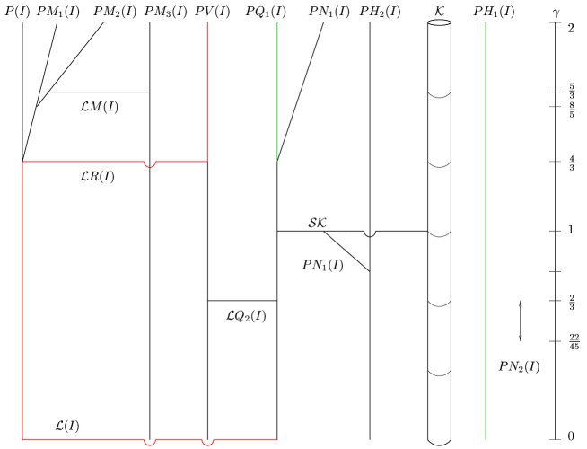
Figure 3: A diagram of the web of equilibrium points. Horizontal lines are bifurcation sets; all are line bifurcations except for $\mathcal{S}\mathcal{K,}$ which is a half-sphere. Lines in red are future attractors, while lines in green are past attractors.

We can note one particular thing, the properties of the future attractor points are altered from the general relativistic case. In the brane-world model the dark-radiation term will make the general-relativistic future attractors unstable for $\gamma>\frac{4}{3}$. Thus, both the local and global properties of the phase space are altered on passing from the general relativistic to the brane-world model. For example, we have brane-world solutions that fly off to infinity in finite time while in the general relativistic case the phase space is compact. Also, the brane-world solutions behave differently in the past. The general relativistic case had no attractors in the past for any $\gamma$. But as we can see, in the brane-world model, there are two past attractors for $\gamma>\frac{4}{3}$ ($PQ_{1}(I)$ and $PH_{1}(I)$) and one for $\gamma\leq\frac{4}{3}$ ($PH_{1}(I)$).

The importance of these fixed points can be expressed in the case $\gamma>\frac{4}{3}$ by the following theorem:

Theorem

Let $p$ be a point in the configuration space $\mathcal{M}$ satisfying the constraint (113), and let $s_{p}(\tau)$ be the maximally extended solution satisfying the equations of motion such that $s_{p}(0)=p$. Then for $\gamma>\frac{4}{3}$ there exists a compact region $C\subset\mathcal{M}$ and a $\tau_{0}$ such that for every $t<\tau_{0}$ then $s_{p}(t)\in C$.

Proof:

Consider the compact region ${\cal F}\subset{\cal M}$ given by $\Sigma=\Sigma_{+}^{2}+\Sigma_{A}^{2}+\Sigma_{B}^{2}+\Sigma_{C}^{2}\leq\Sigma^{*}>1$, $\Omega\leq\Omega^{*}>0$, $\omega\leq\omega^{*}>\sqrt{6}$, $R\leq R^{*}>0$, $H\leq H^{*}>\sqrt{\frac{8}{3}}$ and assume that $\gamma>\frac{4}{3}$. For $\Sigma>1$ we have $\Sigma>|\Sigma_{+}|$ and

$$\Sigma^{\prime} = 2(q-2)\Sigma+6R\Sigma_{+}-\left[(3\gamma-2)\omega H+4H^{2}\right]\Sigma_{+}$$ (114)

$$\geq 2(\Sigma-1)\Sigma+6R\Sigma_{+}+\Sigma\left[\frac{1}{2}H^{2}-\frac{1}{2}(3\gamma-4)\omega H+\frac{1}{3}\omega^{2}\right]$$

$$\geq 2(\Sigma-1-6R)\Sigma$$

because the polynomial in $\omega$ and $H$ inside the square brackets is positive definite for $\gamma\in[\frac{4}{3},2]$. Similarly, for $H\geq H^{*}$ we have

$$H^{\prime}\geq 12\left(H^{*}-\sqrt{\frac{8}{3}}\right)$$ (115)

and for $\omega\geq\omega^{*}$ we have

$$\omega^{\prime}\geq(3\gamma-2)\left(\frac{(\omega^{*})^{2}}{6}-1\right)\omega^{*}$$ (116)

These equations ensures that the variables $H$ and $\omega$ are finite in the past. We also have for $H\neq 0$

$$\left(\frac{R}{H}\right)^{\prime}=(1+q)\left(\frac{R}{H}\right)\geq 2\left(\frac{R}{H}\right)$$ (117)

Integrating yields the bound $\frac{R(\tau)}{H(\tau)}\leq\frac{R(0)}{H(0)}e^{2\tau}$ for $\tau<0$. Hence, in the past $R$ can be driven arbitrarily close to zero as $\tau\longrightarrow-\infty$ since $H$ is bounded. Thus for $\Sigma>\Sigma^{*}$, $\Sigma^{\prime}>0$ for some time in the past. Hence, $\Sigma$ is bounded in the past too. Similarly, for $\omega\neq 0$, $\Omega$ can also be driven arbitrarily close to zero. Thus in this case, the region ${\cal F}$ is sufficient and we can set $C={\cal F}$.

If $H=0$ (which is an invariant solution subspace) the equation for $V$ is

$$V^{\prime}=(2q-2)V$$ (118)

which after a rearranging yields

$$(\ln|V|)^{\prime}=2q-2\geq 0$$ (119)

Thus $V$ is bounded in the past, and according to the constraint equation all of the other variables have to be as well.

If $\omega=0$ but $H>0$, then $\Omega^{\prime}\geq(3\gamma-4)(\Omega^{*}-1)\Omega^{*}>0$ for $\Omega>\Omega^{*}>1$ which makes $\Omega$ bounded in the past.

The theorem now follows from this analysis. $\blacksquare$

This theorem shows that the solution cannot fly off to infinity as $\tau\longrightarrow-\infty$. With some amendments, we believe that the behaviour at the initial singularity is “well-behaved” for any $\gamma$, even though we have not been able to be prove a similar theorem in that case.

In Figure 2 we have drawn a flow-diagram of the dynamical system. The section shown is a part of the non-physical boundary, and the vector field is projected onto this plane. In Figure 3 the web of equilibrium points are illustrated. We see how the points are connected through bifurcation sets, and it is clear how some branch off from other equilibrium points.

From this analysis we believe that it is very likely that the pure magnetic Bianchi type I brane-worlds do not exhibit chaotic behaviour in the past.

5 Discussion

In this paper we have investigated pure magnetic Bianchi type I brane-worlds. We found asymptotic forms for the solutions near the initial singularity for different configurations of matter, magnetic field and shear anisotropy.. We also checked whether there are any equilibrium points that could serve as a past attractor for the generic solutions. For $\gamma>\frac{4}{3}$ we found two such attractors, while in the case $\gamma\leq\frac{4}{3}$ there was one. This may indicate that there can be no chaotic behaviour in the generic solutions for a magnetic Bianchi type I brane-world. To the past, the solution can approach the general relativistic case but will only oscillate a finite number of times. The possible initial states of these two equilibrium points, correspond to two different non general-relativistic models, one of them appears to be previously unknown.

When we investigated the various equilibrium points, we noted that all of the future stable general-relativistic points were unstable in the brane-world scenario for $\gamma>\frac{4}{3}$. Another major difference between the two cases is that the configuration space is non-compact for the brane-world solutions. We found solutions that fled to infinity in a finite coordinate time, and found that the non-local energy $\mathcal{U}$ can become arbitrary large (and even negative) and so presents a major obstacle to this sort of analysis.

The models examined in this paper are based upon the simplest anisotropic universes. It remains to be seen what new features might emerge from a study of the general case. However, we know that in the magnetic case (in contrast to the non-magnetic situation) many of the features of the general anisotropic universe are present in the simple type I model.

Note:

After this paper was completed and submitted, a similar and independent work by Alan Coley appeared [32, 33] addressing some of the same issues as we have done in this paper.

References

- [1] L. Randall and R. Sundrum, Phys. Rev. Lett. 83, 4690 (1999)
- [2] L. Randall and R. Sundrum, Phys. Rev. Lett. 83, 3370 (1999)
- [3] T. Shiromizu, K.I. Maeda, and M. Sasaki, Phys. Rev. D 62, 024012 (2000)
- [4] J.D. Barrow and R. Maartens, gr-qc/0108073.
- [5] A. Campos and C. F. Sopuerta, Phys. Rev. D 63, 104012 (2001)
- [6] A. V. Toporensky, Class. Quant. Grav. 18, 2311 (2001)
- [7] M. G. Santos, F. Vernizzi and P. G. Ferreira, hep-ph/0103112.
- [8] A. Campos and C. F. Sopuerta, astro-ph/0102355.
- [9] C. Chen, T. Harko and M. K. Mak, hep-th/0103240.
- [10] R. Maartens, V. Sahni and T.D. Saini, Phys. Rev. D 63, 063509 (2001)
- [11] J. D. Barrow, Phys. Rev. D 55, 7451 (1997)
- [12] J.D. Barrow, Phys. Rev. D51, 3113 (1995)
- [13] J.D. Barrow and R. Maartens, Phys. Rev. D 59, 043502, (1998)
- [14] V. A. Ruban, Sov. Astron. 26 632 (1982)
- [15] S. Hervik, Class. Quant. Grav. 17, 2765 (2000)
- [16] V. G. LeBlanc, Class. Quantum Grav. 14, 2281 (1997)
- [17] B. L. Spokoiny, Phys. Lett. A 81, 493 (1981)
- [18] V. A. Belinsky, I. M. Khalatnikov and E. M. Lifshitz, Adv. Phys. 19, 525 (1970)
- [19] J.D. Barrow, Phys. Rev. Lett. 46, 963 (1981)
- [20] J.D. Barrow, Phys. Reports 85, 1 (1982)
- [21] D. Chernoff and J.D. Barrow, Phys. Rev. Lett. 50, 134 (1983)
- [22] J. Demaret, M. Henneaux, and P. Spindel, Phys. Lett. B 164, 27 (1985)
- [23] T. Damour, M. Henneaux, B. Julia and H. Nicolai, Phys. Lett. B 509, 323 (2001)
- [24] T. Damour and M. Henneaux, Phys.Rev.Lett. 86, 4749-4752 (2001)
- [25] J.D. Barrow and K. Kunze, Phys. Rev. D 55, 623 (1997)
- [26] C. Tsagas and J.D. Barrow, Class. Quantum Gravity 15, 3523 (1998)
- [27] C. Tsagas and J.D. Barrow, Class. Quantum Gravity 14, 2539 (1997)
- [28] L. P. Hughston and K. J. Jacobs, Astrophys. J. 160, 147 (1970)
- [29] R. Maartens, gr-qc/0101059.
- [30] R. Maartens, Phys. Rev. D 62, 084023 (2000)
- [31] P. Binètruy, C. Deffayet and D. Langlois, Nucl. Phys. B565, 269 (2000)
- [32] A. Coley, hep-th/0110049
- [33] A. Coley, hep-th/0110117