Conditional probabilities in Ponzano-Regge minisuperspace

Abstract

We examine the Hartle-Hawking no-boundary initial state for the Ponzano-Regge formulation of gravity in three dimensions. We consider the behavior of conditional probabilities and expectation values for geometrical quantities in this initial state for a simple minisuperspace model consisting of a two-parameter set of anisotropic geometries on a $2$-sphere boundary. We find dependence on the cutoff used in the construction of Ponzano-Regge amplitudes for expectation values of edge lengths. However, these expectation values are cutoff independent when computed in certain, but not all, conditional probability distributions. Conditions that yield cutoff independent expectation values are those that constrain the boundary geometry to a finite range of edge lengths. We argue that such conditions have a correspondence to fixing a range of local time, as classically associated with the area of a surface for spatially closed cosmologies. Thus these results may hint at how classical spacetime emerges from quantum amplitudes.

I Introduction

Analysis of quantum behavior is usually guided by insight into the classical dynamics of the system. However, this connection is not straightforward in the context of quantum gravity. Classical general relativity is explicitly described in terms of a coordinate system; in particular, the evolution of geometry is given as a function of a time coordinate. However, the quantum mechanics of gravity result in a wavefunction in which there is no explicit dependence on time. Rather, the classical idea of the time evolution of a geometry is expected to emerge from the form of the wavefunction itself. But how and under what conditions? Furthermore, how can information characterizing our classical spacetime such as homogeneity and isotropy be extracted from such a wavefunction?

Obtaining answers to such questions rests not only on knowing the correct quantum theory and initial conditions for the early universe, but also on understanding how to extract from the resulting wavefunction quantities that correspond to the properties of classical spacetime [1]. Indeed, this issue has been key in the study of quantum cosmology. Much exploratory work on the likelihood of isotropy and other observed properties of the universe has been done in the context of both semiclassical general relativity and minisuperspace models. (cf. [2] and references therein.) In addition, various authors [3, 4, 5, 6] have proposed an interpretation of quantum mechanics applicable to closed systems without external observers based on the consistent histories approach to quantum mechanics. This approach has been applied to the study of simple quantum systems related to gravity (cf. [7, 8, 9, 10]) with interesting results.

These suggestive avenues of research have been carried out in the context of a theory of quantum dynamics based on classical general relativity. However, it is generally accepted that this theory is not itself a correct high energy description of quantum gravity; rather it is expected to be an effective theory that corresponds to the correct theory of quantum gravity only in the low energy limit. Furthermore, computations with this effective theory can only be carried out in simple minisuperspace models, in the semiclassical limit, or with other approximation techniques. Therefore it is useful to find other contexts in which we can probe the issues of how to associate the properties of classical spacetimes with quantum states. The Ponzano-Regge theory of gravity may provide one such context.

In 1968, Ponzano and Regge [11] noted an equivalence of the $6j$-symbols for spin to the 3-dimensional Regge action for gravity [12]. They used this equivalence to formulate the partition function for 3-dimensional gravity in terms of a product of $6j$-symbols. This provided a well-formulated, calculable theory of 3-dimensional quantum gravity based on the sum over histories approach to quantum mechanics. Turaev and Viro [13] showed that a generalization of this theory formulated in terms of quantum $6j$-symbols provided new 3-manifold invariants. Ooguri [14] demonstrated that the Ponzano-Regge partition function is equivalent to Witten’s 2+1 formulation of gravity [15] on closed orientable manifolds. Barrett and Crane [16] pointed out that the Biedenhorn-Elliot identity for $6j$-symbols yields a discrete version of the Wheeler-de Witt equation, thereby giving further insight into the relation of Ponzano-Regge theory to 3-dimensional gravity.

Clearly, Ponzano-Regge theory is a potentially useful testing ground for the issues involved in the emergence of classical spacetime and the prediction of isotropy from the wavefunction of the universe. As the theory provides a large number of geometrical degrees of freedom, it yields quantum amplitudes for boundary geometries without any assumption of symmetry. Furthermore, its discrete nature means that it is particularly amenable to numerical analysis. However, in order to implement such studies, one must still understand how to formulate and interpret physical quantities in this theory.

As a modest step toward this goal, this paper examines the formulation of conditional probabilities and expectation values of geometrical quantities in a minisuperspace model of Ponzano-Regge theory. In particular, these quantities are computed in the Hartle-Hawking initial state (cf. [17]) for simple two-parameter anisotropic boundary geometries defined on the surface of a single tetrahedron. These models are useful in that the expectation values can be calculated exactly. We find that a key issue in analyzing and interpreting such expectation values is the role of the cutoff used in the formulation of quantum amplitudes in Ponzano-Regge gravity. We find that the expectation values of edge lengths are linearly proportional to this cutoff. We also find that certain, but not all, expectation values of edge lengths that are conditioned on another edge length are in fact cutoff independent. The factor determining cutoff independence is whether or not the condition imposed restricts the histories yielding the dominant contribution to the expectation value to those with support on a finite region in the interior of the configuration space. We observe that such conditioned histories have a natural description in terms of intrinsic time. We conclude with a discussion of these results and their implications.

II Ponzano-Regge gravity

We begin with the definitions of the $6j$-symbol and the Ponzano-Regge wavefunction. This material is available widely in the literature (see, for example [11], and the generalization in [13]), but in varied notation; we summarize it here for convenience.

Let $j_{1}$, $j_{2}$, $j_{3}$, $j_{4}$, $j_{5}$, $j_{6}$ be non-negative integers or half-integers. An unordered $3$-tuple $(j_{a},j_{b},j_{c})$ is said to be admissible if the triangle inequalities, i.e., ${|j_{b}-j_{c}|}\leq{j_{a}}\leq{j_{b}+j_{c}}$ etc., are met and if the sum $j_{a}+j_{b}+j_{c}$ is an integer. The ordered $6$-tuple $(j_{1},j_{2},j_{3},j_{4},j_{5},j_{6})$ is said to be admissible if and only if each of the unordered $3$-tuples $(j_{1},j_{2},j_{3})$, $(j_{3},j_{4},j_{5})$, $(j_{5},j_{6},j_{1})$, $(j_{2},j_{4},j_{6})$ are admissible. We can associate a $6j$-symbol of $SU(2)$ with the admissible ordered $6$-tuple (cf. [11], [18]):

$$\left\{\matrix{j_{1}&j_{2}&j_{3}\cr j_{4}&j_{5}&j_{6}\cr}\right\}={\sum_{z}}{\frac{(-1)^{z}(z+1)![{\Delta}(j_{1},j_{2},j_{3}){\Delta}(j_{3},j_{4},j_{5}){\Delta}(j_{5},j_{6},j_{1}){\Delta}(j_{2},j_{4},j_{6})]^{1\over{2}}}{(z-n_{1})!(z-n_{2})!(z-n_{3})!(z-n_{4})!(n_{5}-z)!(n_{6}-z)!(n_{7}-z)!}}$$ (1)

where

$$n_{1}=j_{1} + j_{2}+j_{3}\ \ \ \ \ \ n_{2}=j_{3}+j_{4}+j_{5}\ \ \ \ \ \ n_{3}=j_{5}+j_{6}+j_{1}$$ (2)

$$n_{4} = j_{2}+j_{4}+j_{6}\ \ \ \ \ \ \ \ \ \ \ n_{5}=j_{1}+j_{2}+j_{4}+j_{5}$$ (3)

$$n_{6} = j_{2}+j_{3}+j_{5}+j_{6}\ \ \ \ \ n_{7}=j_{1}+j_{3}+j_{4}+j_{6}$$ (4)

and the sum is over all non-negative integer values of $z$ resulting in non-negative arguments of the factorial. The function ${\Delta}(j_{i},j_{j},j_{k})$ is given by

$$\Delta(j_{i},j_{j},j_{k})={(j_{i}+j_{j}-j_{k})!(j_{i}+j_{k}-j_{j})!(j_{j}+j_{k}-j_{i})!\over{(j_{i}+j_{j}+j_{k}+1)!}}\,.$$ (5)

For inadmissible 6-tuples, the $6j$-symbol is defined to vanish.

There is a natural geometric representation of the $6j$-symbol in terms of a $3$-dimensional tetrahedron $t$ (see Figure 1). In particular, we can associate the edges of $t$ with the $j_{a}$’s in the $6j$-symbol as follows. Choose a face on $t$, label the edges of this face by $j_{1}$, $j_{2}$ and $j_{3}$. Next label the edge which shares no vertices with $j_{1}$ by $j_{4}$, the edge which shares no vertices with $j_{2}$ by $j_{5}$ and that which shares no vertices with $j_{3}$ by $j_{6}$. There are clearly two distinct choices of edge for $j_{2}$ or $j_{3}$—they determine the handedness of our labeling. The handedness, however, has no effect on calculations since the corresponding $6j$-symbols are equivalent according to the symmetry

$$\left\{\matrix{j_{1}&j_{2}&j_{3}\cr j_{4}&j_{5}&j_{6}\cr}\right\}=\left\{\matrix{j_{1}&j_{3}&j_{2}\cr j_{4}&j_{6}&j_{5}\cr}\right\}\ \,.$$ (6)

The edge length associated with each $j_{a}$ is given by $l_{a}={j_{a}+{1\over 2}}$, $a=1,2,...,6.$ Note that the requirement that the 3-tuples be admissible guarantees that the edges $l_{a}$, $l_{b}$, $l_{c}$ form a closed triangle of non-zero area. The triangle inequalities do not, however, guarantee the associated tetrahedron has real volume; it is possible to construct hyperflat tetrahedra, that is tetrahedra with negative volume squared $V^{2}$ where

$$V^{2}={1\over{2^{3}(3!)^{2}}}\left|\matrix{0&l_{4}^{\ 2}&l_{5}^{\ 2}&l_{6}^{\ 2}&1\cr l_{4}^{\ 2}&0&l_{3}^{\ 2}&l_{2}^{\ 2}&1\cr l_{5}^{\ 2}&l_{3}^{\ 2}&0&l_{1}^{\ 2}&1\cr l_{6}^{\ 2}&l_{2}^{\ 2}&l_{1}^{\ 2}&0&1\cr 1&1&1&1&0\cr}\right|\,.$$ (7)

This occurs when the sum of angles between three edges forming a vertex is greater than $2\pi$. Clearly, tetrahedra with non-negative $V^{2}$ can be embedded in a 3-dimensional Euclidean space, while the same can not be done with tetrahedra with negative $V^{2}$. However, the ${V}^{2}<0$ tetrahedra can be embedded in a 3-dimensional Lorentzian space (cf. [19]).

For large edge lengths, the $6j$-symbol corresponds to the gravitational action through the relation

$$\left\{\matrix{j_{1}&j_{2}&j_{3}\cr j_{4}&j_{5}&j_{6}\cr}\right\} \simeq \frac{1}{\sqrt{12\pi V}}\cos(I+\frac{\pi}{4})$$ (8)

$$I = \sum_{k}l_{k}\theta_{k}$$ (9)

where $\theta_{k}$ is the angle between the outward-directed normals to the two faces that intersect at edge $l_{k}$. $I$ is the contribution of the tetrahedron to the 3-dimensional Regge action[12] in units where $8\pi G=1$.

Next, we give the Ponzano-Regge partition function for compact 3-manifolds, or equivalently, the Hartle-Hawking no-boundary initial state for Ponzano-Regge theory. Let $T[M]$ be a tessellation of a compact $3$-manifold $M$ with boundary ${\partial}M$. (A definition of a tessellation is provided in the Appendix.) Also let $T[{\partial}M]$ be the restriction of the tessellation of $M$ to ${\partial}M$. Denote the sets of vertices, edges, triangles and tetrahedra in $T[M]$ as $S_{0}$, $S_{1}$, $S_{2}$ and $S_{3}$ respectively. Similarly denote the sets of vertices, edges, and triangles in $T[{\partial}M]$ as $B_{0}$, $B_{1}$, $B_{2}$ respectively. Let let $s_{m}$ be the cardinality of the set $S_{m}$ and $b_{m}$ that of the set $B_{m}$.

Next, let $K$, the cutoff, be a non-negative integer or half-integer. Let $\phi$ be an assignment of a non-negative integer or half-integer value $j_{i}\leq{K}$ to each edge in $S_{1}$. If every 6-tuple associated to a tetrahedron in $S_{3}$ by the assignment $\phi$ is admissible, then $\phi$ is termed an admissible assignment. Let $\{J_{i}\}$ denote the set of integer and half-integer values of edges in $B_{1}$. Note that $\{J_{i}\}$ is a subset of the set of all edges $\{j_{i}\}$. Labeling the edges in the boundary by indices $1,\ldots b_{1}$, the Ponzano-Regge wavefunction for a compact $3$-manifold is given by

$$\Psi[M,\{J_{i}\}] = {\lim_{{K}\to{\infty}}}\Psi_{K}[M,\{J_{i}\}]$$ (10)

$$\Psi_{K}[M,\{J_{i}\}] = \sum_{\phi}\Lambda^{-(s_{0}-b_{0})}\prod_{i=1}^{b_{1}}(-1)^{J_{i}}(2J_{i}+1)^{{1\over{2}}}\prod_{i=b_{1}+1}^{s_{1}}(-1)^{2j_{i}}(2j_{i}+1)\prod_{n=1}^{s_{3}}[t_{n}]\,.$$ (11)

where the sum is over all admissible assignments $\phi$, $[t_{n}]$ is

$$[t_{n}]=(-1)^{-(j_{a}+j_{b}+j_{c}+j_{d}+j_{e}+j_{f})}\left\{\matrix{j_{a}&j_{b}&j_{c}\cr j_{d}&j_{e}&j_{f}\cr}\right\}$$ (12)

in terms of the $6j$-symbol for the $n^{th}$ tetrahedron, and

$$\Lambda=\sum_{p=0,{1\over 2},...,K}(2p+1)^{2}\,.$$ (13)

The term $\Lambda^{-(s_{0}-b_{0})}$ regulates divergences in this expression that appear due to the presence of internal vertices [11]. As a given $6j$-symbol is proportional to the contribution to the path integral amplitude for its associated tetrahedron, the product of $6j$-symbols is equivalent to the path integral amplitude for a given simplicial geometry. Thus each admissible assignment of edge lengths corresponds to a history in the path integral. The sum over admissible assignments is then a sum over histories for 3-d gravity. Note that we can associate a classically allowed history as one composed of $6j$-symbols corresponding to tetrahedra of non-negative $V^{2}$, and a classically forbidden history as that containing one or more tetrahedra of negative $V^{2}$. Finally, observe that the wavefunction will vanish if there is no admissible assignment $\phi$.

For closed 3-manifolds, $\{J_{i}\}=\emptyset$, and equation (11) reproduces the usual partition function for Ponzano-Regge theory (cf. [11, 13]). Indeed, the wavefunction (11) satisfies a natural composition law: given tessellations of two $3$-manifolds $M$ and $N$ with the same boundary, $\partial M=\partial N$, such that each boundary has identical tessellation, $T[{\partial}M]=T[{\partial}N]$, then

$$\Psi[M\cup N] = {\lim_{{K}\to{\infty}}}\Psi_{K}[M\cup N]$$ (14)

$$\Psi_{K}[M\cup N] = {\sum_{\{\{J_{i}\}|{J_{i}}\leq{K}\}}}\Lambda^{-b_{0}}{\Psi}_{K}[M,\{J_{i}\}]{\Psi}_{K}[N,\{J_{i}\}]\,.$$ (15)

The inclusion of $\Lambda^{-b_{0}}$ in the measure regulates divergences appearing from the fact that the boundary vertices are now internal. This composition law also reproduces the usual partition function for closed 3-manifolds.

The expectation value of an operator $O$ is naturally formulated as

$$<{\cal O}>=\frac{1}{\Psi[M\cup M]}{\lim_{{K}\to{\infty}}}{\sum_{\{\{J_{i}\}|{J_{i}}\leq{K}\}}}\Lambda^{-b_{0}}{\Psi}_{K}[M,\{J_{i}\}]{O}{\Psi}_{K}[M,\{J_{i}\}]\,.$$ (16)

This definition can be viewed as the calculation of $O$ from the generating functional in Ponzano-Regge theory for which the initial and final states are identical.

An equivalent form of this expectation value for suitably convergent numerator and denominator in (16), is given by

$$<{\cal O}> = {\lim_{{K}\to{\infty}}}<O>_{K}$$ (17)

$$<O>_{K} = \frac{1}{\Psi_{K}[M\cup M]}{{\sum_{\{\{J_{i}\}|{J_{i}}\leq{K}\}}}\Lambda^{-b_{0}}{\Psi}_{K}[M,\{J_{i}\}]{O}{\Psi}_{K}[M,\{J_{i}\}]}$$ (18)

where $\Psi_{K}[M\cup M]$ is given by (15). It is important to note that both the above expressions are purely formal; the numerator and denominator may not necessarily converge in either. However, it is reasonable to expect that physically meaningful expectation values are convergent. Therefore, examination of the properties of such expressions as $K\to\infty$ is the subject of this paper. For notational convenience, as all expectation values computed in the subsequent sections will be cutoff expectation values of form (18) unless otherwise noted, we will suppress the subscript $K$, e.g. $<O>_{K}\equiv<O>$.

The simplest example of the Hartle-Hawking no-boundary initial state is given by the tessellation of a $3$-ball $B^{3}$ with $2$-sphere boundary as a single tetrahedron (see Figure 1). The geometry of its boundary is completely specified by six independent edges. The wavefunction for this case is just

$$\Psi[B^{3},\{J_{i}\}] = {\lim_{{K}\to{\infty}}}\Psi_{K}[B^{3},\{J_{i}\}]$$ (19)

$$\Psi_{K}[B^{3},\{J_{i}\}] = \biggl{[}\prod_{i=1}^{6}(2J_{i}+1)^{{1\over{2}}}\biggr{]}\left\{\matrix{J_{1}&J_{2}&J_{3}\cr J_{4}&J_{5}&J_{6}\cr}\right\}\,.$$ (20)

The cutoff wavefunction and the limiting wavefunction are manifestly equivalent in this case. However, although the wavefunction is cutoff independent, expectation values of geometrical quantities such as edge lengths will not necessarily be so.

III Isotropic minisuperspace

We will begin by considering the simplest minisuperspace model, that of the isotropic boundary. In this model, we restrict all edges to have equal value $l_{X}=X+{1\over 2}$. Then,

$$\Psi[B^{3},\{X\}]=\Psi_{K}[B^{3},\{X\}]=(2X+1)^{3}\left\{\matrix{X&X&X\cr X&X&X\cr}\right\}\,.$$ (21)

It follows from the admissibility conditions that $\Psi[B^{3},\{X\}]$ vanishes unless $X$ is integer. Figure 2 displays this oscillatory wavefunction; it is apparent that it contains no striking structural features.

Next, we examine expectation values in this minisuperspace model. We do so by first calculating the cutoff expectation values in this model, then analyzing their behavior as $K\to\infty$. The cutoff expectation value of the edge length is given by

$$<l_{X}>={\sum_{X=0}^{K}{(X+{1\over 2}){|{\Psi_{K}[B^{3},\{X\}]}|^{2}}}\over{\sum_{X=0}^{K}{|{\Psi_{K}[B^{3},\{X\}]}|^{2}}}}\,.$$ (22)

The uncertainty in the edge length ${\Delta}l_{X}=\sqrt{<(l_{X}-<l_{X}>)^{2}>}$ can be calculated similarly. We evaluate these expressions exactly using computer assistance. Figure 3 displays the results of these calculations for values of ${0}\leq{K}\leq{200}$. The results of linear least-squares fits to these data yield

$$<l_{X}> = ({0.8003}\pm{0.0003})K+({0.55}\pm{0.04})$$ (23)

$${\Delta}l_{X} = ({0.16356}\pm{0.00007})K+({0.081}\pm{0.008})\,.$$ (24)

Observe that the linear dependence on the cutoff appears in computations of expectation values for the edge length of an isotropic tetrahedron embedded in flat 3-dimensional Euclidean space. As the volume of a tetrahedron with edge $l$ is $V={l^{3}\over{6\sqrt{2}}}$, the unnormalized probability for the edge to have length between $l$ and $l+dl$ is $dV={l^{2}\over{2\sqrt{2}}}dl$. If we calculate the expected edge length and its uncertainty using this distribution cut off at a maximum edge length $K$,

$${<l>}=\frac{1}{V_{K}}\int\limits_{0}^{K}\frac{l^{3}dl}{2\sqrt{2}}={{3}\over{4}}K\ \ \ {\rm{where}}\ \ \ V_{K}=\int\limits_{0}^{K}\frac{l^{2}dl}{2\sqrt{2}}\,.$$ (25)

Similarly,

$${{\Delta}{l}}={\sqrt{{3}\over{80}}}K\,.$$ (26)

Furthermore, it is easy to see that the expectation value for the edge length of any isotropic 3-dimensional solid will exhibit such linearity.

IV Anisotropic minisuperspace

Clearly, the isotropic edge length expectation values are cutoff dependent. But do there exist any expectation values which are not dependent on $K$? We address such questions in this section using the simplest model possible to do so, the Hartle-Hawking initial state with boundary consisting of an anisotropic tetrahedron in which the six edges can take two distinct lengths. There are five types of this geometry characterized by the $j$-values and symmetries of the $6j$-symbol. Figure 4 illustrates the five types.

Due to the formulation of the wavefunction in terms of edge lengths, the most convenient conditional expectation value to compute is the expectation value of one edge length for a fixed value of the other. We will do so below for the type A tetrahedron, then summarize the results for the remaining four types.

The type A tetrahedron has an equilateral triangle as its base and three isosceles triangles meeting at its vertex. The wavefunction is

$$\Psi[B^{3},\{X,Y\}_{\rm{A}}]=\Psi_{K}[B^{3},\{X,Y\}_{\rm{A}}]=(2X+1)^{3\over{2}}(2Y+1)^{3\over{2}}\left\{\matrix{X&X&X\cr Y&Y&Y\cr}\right\}\,,$$ (27)

where $X=0,1,2,...,K$, and $Y=0,{1\over{2}},1,...,K$. Figure 5 shows $\Psi[B^{3},\{X,Y\}_{\rm{A}}]$ as a function of $X$ and $Y$. Notice that $\Psi[B^{3},\{X,Y\}_{\rm{A}}]$ vanishes for $X>2Y$ as such configurations are inadmissible, a feature not found in the isotropic case. This vanishing only occurs for certain classically forbidden histories, that is, those with $V^{2}<0$. This feature is easily understood in terms of the geometry of the tetrahedron; given the length $l_{Y}$ of the three edges forming the peak of the tetrahedron, the triangle inequalities fix a maximum length for the three edges forming its base.

Now the minisuperspace expression for a cutoff expectation value, for example the edge length $l_{X}$, is given by

$$<l_{X}>={{\sum_{X,Y=0}^{K}(X+{1\over{2}})|\Psi_{K}[B^{3},\{X,Y\}_{\rm{A}}]|^{2}}\over{\sum_{X,Y=0}^{K}|\Psi_{K}[B^{3},\{X,Y\}_{\rm{A}}]|^{2}}}\,,$$ (28)

where $X=0,1,2,...,K$ and $Y=0,{{1}\over{2}},1,...,K$. Exact evaluations of such expressions using computer assistance show that, as expected, the cutoff expectation values of edge lengths are again linear in $K$; Figure 6 displays these results for the type A tetrahedron and Table II gives the results of least squares fits to the data. The slope of the linear dependence in $K$ differs somewhat from that of the isotropic calculation for both $X$ and $Y$ edges as well as from each other. This difference is presumably due to the anisotropy of the tetrahedron which is explicitly reflected in the nested summation over the $X$ and $Y$ edges.

Table I summarizes configurations for the five different two-parameter anisotropic tetrahedral types. The computed unconditioned expectation values and uncertainties for all the anisotropic tetrahedra are linear in cutoff $K$. Table II displays the result of linear fits to these data. Note that in carrying out the evaluation of cutoff expectation values of form similar to (28), summations over $X$ and $Y$ may or may not include half-integer values depending on whether or not the admissibility conditions allow these configurations. Again, Table I summarizes the pertinent details. All unconditioned expectation values and uncertainties are linear with coefficients which vary slightly from each other and the isotropic values. Also observe that the coefficients of type B are equal, as expected from the symmetry under exchange of labeling $X$ and $Y$.

As for the isotropic case, the linear dependence on the cutoff $K$ appears in computations for all the anisotropic tetrahedra embedded in flat 3-dimensional Euclidean space. The volume of an anisotropic tetrahedron with edges $l_{X}$ and $l_{Y}$ is calculated as $V=\int P(l_{X},l_{Y})dl_{X}dl_{Y}$, where $P(l_{X},l_{Y})$ is a homogeneous polynomial of degree one that vanishes identically for classically inadmissible configurations. The unconditional expected edge length $<l_{X}>$ is therefore

$${<l_{X}>}=\frac{1}{V_{K}}\int\limits_{l_{Y}=0}^{K}\int\limits_{l_{X}=0}^{K}l_{X}P(l_{X},l_{Y})dl_{X}dl_{Y}\propto K\ \ \ {\rm{where}}\ \ \ V_{K}=\int\limits_{l_{Y}=0}^{K}\int\limits_{l_{X}=0}^{K}P(l_{X},l_{Y})dl_{X}dl_{Y}\propto K^{3}\,.$$

Similarly,

$$\Delta l_{X}\propto K\,.$$

We next consider conditional expectation values for the anisotropic tetrahedron. Fixing a value of $l_{Y}$, the cutoff conditional expectation value of $l_{X}$ is given by

$${<l_{X}|_{l_{Y}}>}={\sum_{X=0}^{K}{(X+{1\over 2}){|{\Psi_{K}[B^{3},\{X,Y\}_{\rm{A}}]}|}^{2}}\over{\sum_{X=0}^{K}{|{\Psi_{K}[B^{3},\{X,Y\}_{\rm{A}}]}|}^{2}}}\,,$$ (29)

where $X=0,1,2,...,K$ and $l_{Y}=Y+\frac{1}{2}$ is a fixed integer or half-integer value.

One sees that, unlike $<l_{X}>$, ${<l_{X}|_{l_{Y}}>}$ is independent of $K$ for edge lengths $l_{Y}$ such that $Y<\frac{K}{2}$ (see Figure 7(b)). When cutoff independent, $<l_{X}|_{l_{Y}}>$ clearly exhibits linear dependence on $l_{Y}$ (see Figure 7(a)). For $Y\geq\frac{K}{2}$, ${<l_{X}|_{l_{Y}}>}$ is cutoff dependent and also oscillates away from its previous linear relationship to $l_{Y}$ (as seen in Figure 7(a)). Similarly, ${\Delta}{l_{X}|_{l_{Y}}}$ is linearly dependent on $l_{Y}$ while cutoff $K$ independent and exhibits more complicated behavior for $Y\geq\frac{K}{2}$ (again, see Figure 7). Note that ${<l_{X}|_{l_{Y}}>}$ and ${\Delta}{l_{X}|_{l_{Y}}}$ show little deviation from linearity for the classically forbidden values of $l_{Y}$. That is, it appears the functions are nearly constant for ${(K+{{1}\over{2}})}>{\sqrt{3}{l_{Y}}}$ where values $l_{X}>{\sqrt{3}{l_{Y}}}$ enter the summation. Classically forbidden histories therefore contribute comparatively little to these expectation values.

A study of the conditional expectation values and uncertainties for the remaining tetrahedral types verifies the correspondence of a constraining condition and a $K$ independent conditional expectation value for the appropriate range of the constraining edge length. In Table I we give the ranges that the area-constraining edge lengths enforce. Note that both $X$ and $Y$ edges of the type B and C tetrahedra result in area-constraining conditions. The results of exact evaluations are displayed in Figures 9 and 10. Observe that, when cutoff $K$ independent, the resulting expectation values and uncertainties are linear functions of the constraining edge length. Table III contains the results of linear fits to cutoff independent regions of the calculated values. All linear regions of conditional expectation values and uncertainties have coefficients which vary slightly between the tetrahedral types. Also observe that the coefficients of type B are again equal, as expected from the symmetry under exchange of labeling $X$ and $Y$.

V Discussion

When we examine the results for unconditioned expectation values for the isotropic and anisotropic cases, we find explicitly linear cutoff dependence. However, when we look at conditioned expectation values, we find two strikingly different behaviors—sometimes the results are cutoff independent and linearly varying with the length of the conditioning edge, while at other times the calculated quantities are dependent on the cutoff and not linear in the conditioning edge length. We now interpret these behaviors.

A Unconditional Probabilities

We already observed that the linearity in $K$ for the unconditioned cutoff expectation values of edge length is what one would expect from a classical probability distribution. This correspondence with a classical distribution is not surprising given the importance of classical solutions in the continuum formulation of 2+1 gravity [15]. However, this observation does not address the role of the cutoff $K$ and its physical significance.

There are two natural interpretations. First, note that no physical scale has been set by Ponzano-Regge gravity; the wavefunction contains no parameters other than that of the edge value $X$. In particular, observe that in the context of the semiclassical limit (9), a rescaling of the edge lengths $l_{k}\to\lambda l_{k}$ in the classical Regge action (9) results in a rescaling, $I\to\lambda I$. This scaling $\lambda$ can be absorbed by redefining the length scale set by $8\pi G$. A change of edge length can thus be thought of as a change of this length scale to another value. Therefore, even though the gravitational constant is a length scale in the problem, one cannot vary it independently. Consequently there is no physical parameter to set a length scale that is independent of the cutoff $K$; $K$ is the only accessible scale parameter in the cutoff amplitudes. A change in $K$ in the calculation of this expectation value can therefore be viewed as a rescaling of units. As the cutoff expectation value scales linearly with $K$, its value is not physical.

Alternately, these results can also be interpreted in terms of intrinsic time. It is well-known that the position of a closed spatial hypersurface of a given geometry in a spacetime with closed spatial topology corresponds to a local time variable. For example, consider the maximal extension of 2+1 de Sitter spacetime. It has topology $S^{2}\times R$ and metric $ds^{2}=-dt^{2}+{\alpha}^{2}{\cosh}^{2}({\alpha}^{-1}t)d\Omega^{2}$ where $d\Omega^{2}$ is the unit round metric on the $2$-sphere. A round $2$-sphere of radius $R$ corresponds to only two spatial slices of this spacetime—those at $t=\pm\alpha\cosh^{-1}({\alpha}^{-1}R)$. Thus the spatial geometry of the $2$-sphere, in this case its area, encodes information about its local time position. In quantum cosmology, this classical association corresponds to an intrinsic time variable formed from the geometry of this spatially closed hypersurface (cf. [20], [21]).

In the case at hand, such a local intrinsic time would be associated with the area of the tetrahedron. For the isotropic tetrahedron, the area is proportional to the square of the edge length. In the context of quantum cosmology, expectation values of the type calculated here can be thought of as averages over time. The choice of cutoff $K$ then corresponds to fixing a final time. Clearly, as the wavefunction (21) is not localized in $X$, unless the operators computed are themselves localized, their expectation values will depend on the cutoff. Here, the linear dependence of expectation values on $K$ indicates that this value does not reflect a geometrical property of the surface, but rather its time dependence.

Note that these interpretations, while somewhat different, are in fact compatible. The second simply associates the concept of final time to the cutoff of the problem. Although this case of the isotropic boundary tetrahedron is particularly simple, it clearly delineates the relation in Ponzano-Regge theory.

Of course, one can also interpret the linear relation to $K$ as itself indicative of certain characteristics of the system. The correspondence of (24) to (25), (26) point to a correspondence of the quantum dynamics of the cutoff wavefunction to a classical evolution describing flat space. In this viewpoint, the fact that the coefficients $K$ in (24) differ slightly from those of the classical distribution (25), (26) might be expected from the oscillatory nature of the wavefunction (as displayed in Figure 2). Such a view of cutoff expectation values treats the cutoff formulation of Ponzano-Regge theory as relevant in its own right. However, this cutoff theory cannot be assumed to be equivalent to Ponzano-Regge theory. In particular, the tessellation independence of Ponzano-Regge amplitudes, a property explicitly dependent on the $K\to\infty$ limit, will not be achieved in the cutoff theory. Consequently, the linear relations observed in the cutoff theory may or may not reflect properties of Ponzano-Regge theory itself.

B Conditional Probabilities

We now examine conditioned expectation values, focusing on ${<l_{X}|_{l_{Y}}>}$ for the type A tetrahedral boundary. Again, the behavior of our results is easily understood from the classical geometry of the tetrahedron. Since all configurations with $X>2Y$ are inadmissible, these configurations have vanishing $\Psi[B^{3},\{X,Y\}_{\rm{A}}]$ (see Figure 5) and thus vanishing probability density. Therefore, if $Y$ is fixed to be less than $\frac{K}{2}$, the conditional probability density, and therefore ${<l_{X}|_{l_{Y}}>}$, will be independent of $K$. If $Y\geq\frac{K}{2}$, then there will be non-vanishing probability density for values of $X=K$. Consequently, the expectation value will exhibit cutoff dependence if they include configurations in the range $Y\geq\frac{K}{2}$. Figure 7 displays the results of these calculations.

Interpreting in terms of intrinsic time, fixing $l_{Y}$ in the calculation of the expectation value restricts the histories that contribute to (29) to those corresponding to a particular range of edge lengths, or equivalently areas of the tetrahedron. As this area corresponds classically to intrinsic time, this restriction amounts to selecting a fixed range of intrinsic time, then computing the time average of the expectation value over this range. Therefore, ${<l_{X}|_{l_{Y}}>}$ yields a result that reflects properties of an edge length associated with a particular bounded time average for a suitable range of $Y$. For this range, the limit $K\to\infty$ of ${<l_{X}|_{l_{Y}}>}$ is well-defined. Therefore such conditional expectation values yield a physically meaningful result.

Interestingly enough, ${<l_{X}|_{l_{Y}}>}$, when well-defined, is linear in $l_{Y}$ (as seen in Figure 7). Now one can repeat the arguments on the lack of another physical scale parameter in the problem to argue that a change in $l_{Y}$ corresponds to a change of scale. This again indicates that the value of ${<l_{X}|_{l_{Y}}>}$ is scale dependent. However, the situation is quite different from the case of the unconditioned calculations. Now, one has independent control over the physical scale and the cutoff needed in the definition of the Ponzano-Regge theory. Therefore, the linearity seen in these expectation values can be taken as physical. Furthermore, one can argue that the linearity of ${<l_{X}|_{l_{Y}}>}$ in $l_{Y}$ demonstrates a physical property of this amplitude, namely that that this quantum amplitude corresponds to a flat space.

Similar to analysis of the unconditioned case, linear dependence on the conditioning edge $l_{Y}$ appears in computations for tetrahedra embedded in flat 3-dimensional Euclidean space. Since the volume of a type A tetrahedron with edges $l_{X}$ and $l_{Y}$ is $V=\frac{{\,l_{X}}^{2}}{12}\sqrt{3{{l_{Y}}^{2}}-{{l_{X}}^{2}}}$, the unnormalized probability for the edge to have length between $l_{X}$ and $l_{X}+dl_{X}$ is

$$dV=\left|\,\frac{\,l_{X}}{6}(3{{l_{Y}}^{2}}-{{l_{X}}^{2}})^{\frac{1}{2}}-\frac{{\,l_{X}}^{3}}{12}(3{{l_{Y}}^{2}}-{{l_{X}}^{2}})^{-\frac{1}{2}}\,\right|\,dl_{X}\,.$$

Calculating the conditional expected edge length $<l_{X}|_{l_{Y}}>$ and uncertainty $\Delta l_{X}|_{l_{Y}}$ we obtain

$${<l_{X}|_{l_{Y}}>}=\frac{1}{V_{l_{Y}}}\int\limits_{0}^{\sqrt{3}l_{Y}}l_{X}dV\simeq 1.23l_{Y}\ \ \ {\rm{where}}\ \ \ V_{l_{Y}}=\int\limits_{0}^{\sqrt{3}l_{Y}}dV\,,$$ (30)

and similarly

$${{\Delta}{l_{X}}|_{l_{Y}}}\simeq 0.498l_{Y}\,.$$ (31)

Again observe that the constants of proportionality for the classical calculation are close to those of the corresponding Ponzano-Regge calculation. As for the unconditioned case, the differences can be attributed to the oscillatory nature of the wavefunction $\Psi[B^{3},\{X,Y\}_{\rm{A}}]$ (as shown in Figure 5).

If the key property yielding cutoff independence is that the condition fixes a bounded range of intrinsic time, then it follows that $<l_{Y}|_{{l_{X}}}>$ and ${\Delta}l_{Y}|_{{l_{X}}}$ should not exhibit this cutoff independence for any range of $l_{X}$. Geometrically, fixing $l_{X}$ does not restrict the range of $l_{Y}$. Hence, this condition will not appropriately restrict the region of non-vanishing probability density. Calculations of these quantities verify this hypothesis (see Figure 8). The expectation value $<l_{Y}|_{{l_{X}}}>$ exhibits cutoff dependence for all values of $l_{X}$. The fact that this expectation value is $K$ dependent implies that it is not well-defined in the $K\to\infty$ limit. Hence the hypothesis that only conditional expectation values for which conditions restricting the range of fixed intrinsic time result in physically meaningful answers is verified. Furthermore, observe that the linear correlations displayed between the cutoff $K$ independent conditional calculations and the constraining edge length are not present in either $<l_{Y}|_{{l_{X}}}>$ or ${\Delta}l_{Y}|_{{l_{X}}}$.

A study of the conditional expectation values and uncertainties for the other anisotropic tetrahedral types verifies this behavior—when cutoff $K$ independent, the resulting expectation values and uncertainties are linear functions of the constraining edge length. Again, Table I gives the ranges that the area-constraining edge lengths enforce. Recall that both $X$ and $Y$ edges of the type B and C tetrahedra result in area-constraining conditions. Once more, Table III contains the resulting linear fits for the appropriate ranges of the constrained edge lengths for all five anisotropic types. These results are consistent with the flat space interpretation as for the type A tetrahedron.

VI Conclusions

This simple study of expectation values on Ponzano-Regge minisuperspace demonstrates the utility of this theory in addressing issues of the emergence and properties of classical spacetime. It is clearly not true that all expectation values that can be formulated for a fixed cutoff value are physically meaningful. It is also clear that not all conditions on such expectation values will yield a cutoff independent result. However, what is significant is the close correspondence between the formulation of conditional expectation values that are cutoff independent quantities—and thus physically meaningful—and conditions that correspond to fixing a finite range of time. Furthermore, the linear nature of these cutoff independent quantities on the constraining edge length is consistent with embedding of the tetrahedron in the classical flat background. These results are not just of mathematical interest, but indicate that Ponzano-Regge theory may be able to provide insight into the formulation of physically interesting expectation values.

Clearly, one can ask whether or not more can be determined from well-defined conditioned expectation values. In particular, expectation values of the form ${<l_{X}|_{l_{Y}}>}$ loosely correspond to the characterization of the isotropy of a universe at a given time. The interesting fact about the results for ${<l_{X}|_{l_{Y}}>}$ is that, as seen in Table III, they are dependent on the boundary tetrahedron type. Therefore, it is not clear that the coefficients of $l_{Y}$ hold much meaning in and of themselves. However, if one chooses to interpret the values relative to the isotropic tetrahedron, it is clear that $\frac{l_{Y}}{2}<{<l_{X}|_{l_{Y}}>}<\frac{3l_{Y}}{2}$. Thus, although the anisotropy of the surface in this interpretation is not zero, it is in some sense small.

What is interesting about these results is the direction in which they point. Ideally, one would like to be able to search for quantities characterizing the emergence of classical spacetime in situations for which it is not so clear what the relevant degrees of freedom are. So what characterizes whether or not the expectation values computed are relevant? From our results, we see that requiring cutoff independence in conditional expectation values is crucial and required for physically meaningful results. Furthermore, these results are compatible with the presence of a localization in intrinsic time.

Given Ooguri’s work [14] demonstrating the equivalence of 2+1 gravity in the Witten variables to Ponzano-Regge theory, it is clearly of interest to ask how our results fit into the issue of appearance of time in 2+1 gravity. To this end, note that, in the continuum theory, the phase space of $SO(2,1)$ holonomies parameterizes the inequivalent flat spacetimes for different topologies in 2+1 gravity. The wavefunctions for 2+1 gravity are functions of suitable projections of this phase space. That is the basis of Witten’s approach—he quantizes gravity using diffeomorphism invariant $SO(2,1)$ holonomy variables [15]. His approach results in a vanishing Hamiltonian and gauge invariant states. Witten’s quantization is therefore time independent. Alternately, Moncrief [22], and Hosoya and Nakao [23] have given a quantization based on Arnowitt-Deser-Misner variables and the York decomposition. In that formulation they use a time variable defined as the trace of the extrinsic curvature $K$. The formulation yields a non-vanishing Hamiltonian and states that are dependent on $K$, i.e. are time dependent. Now, in [24] Carlip compares the Witten quantization to that due to Moncrief, Hosoya and Nakao. Carlip shows that these two quantizations are exactly equivalent for the case of the two-torus, and explicitly constructs a canonical transformation between Moncrief’s and Witten’s variables for that case. Carlip thus demonstrates the possibility of canonically transforming an explicitly time dependent quantum theory of 2+1 gravity to one in which the dependence is hidden in the new variables.

How do our results fit into this picture? Our analysis of Ponzano-Regge theory through the calculation of expectation values is formulated with respect to a fixed boundary. Clearly fixing a boundary corresponds to a fixed slicing. Thus our (discrete) formulation parallels that of Moncrief, Hosoya and Nakao; we expect that our amplitudes to be time dependent (i.e. cutoff dependent) and indeed they are. We found that unconditional expectation values are linear in the cutoff, precisely the dependence that these values have in the classical probability distribution for flat space. The linearity of expectation values is also consistent with uniqueness of the solution for $2$-sphere topology in 2+1 gravity [15]. As the phase space for the $2$-sphere consists of a point, the wavefunction in this formulation is trivial.

However, we also demonstrate that we can extract from these amplitudes physical behavior that is in fact time independent by considering certain conditional expectation values. More convincingly, we found that well-defined conditional expectation values are linear functions of the conditioning edge length. Again this behavior reflects the underlying flat space structure we expect. Part of the utility of our method is that we can extract physical behavior without forming maps between gauge independent and gauge dependent quantizations.

We carried out this analysis in terms of simple minisuperspace models in which all calculations could be carried out exactly. It is important to note that the computation of expectation values in the anisotropic minisuperspace approximation involved a restriction of the sum over edge lengths from six values to two. This restriction will result in a reduction of the degree of divergence of such expressions if no further changes in the measure are carried out. This feature is common to other minisuperspace models as freezing out degrees of freedom typically results in the redefinition of the measure. Clearly, this point indicates that the results we have found are likely qualitative, rather than quantitative. Even so, the issue of the divergence of the expectation values with cutoff will remain in the full Ponzano-Regge theory. It is clearly of interest to study how such results will appear. Given what our minisuperspace results indicate, one can imagine formulating similar conditional expectation values in the full Ponzano-Regge theory, numerically evaluating these using Monte Carlo techniques, and searching for cutoff independence as a signal of a meaningful expectation value with a physical interpretation. Clearly, it is of interest to see whether such conditional measurements have any connection to the emergence of classical spacetime.

Furthermore, it is clearly important to consider such conditional expectation values in the context of other 3-manifold topologies. Ionicioiu and Williams [25] computed amplitudes for 3-manifolds in a closely related theory of Turaev and Viro [13] in which 3-manifold invariants are formulated in terms of a topological field theory. Ooguri [14] related the formulation of the Hartle-Hawking no-boundary initial state on handlebodies to that of a Chern-Simons theory. It is obviously of interest to study the characterization of such solutions in the context of the interpretation of quantum cosmology as their solution space is no longer zero dimensional. So whether or not the Hartle-Hawking wavefunction yields conditional expectation values with special properties is clearly of interest.

A Definitions

In order to concretely define a tessellation, we begin by defining simplices [26]: Let the vertices $v_{1},v_{2},\ldots,v_{n+1}$ be affinely independent points in ${\bf R}^{m}$ where $m\geq n+1$. An n-simplex $\sigma^{n}$ is the convex hull of these points:

$$\sigma^{n}=\{x\in{\bf{R}}^{m}|x=\sum_{i=1}^{n+1}\lambda_{i}v_{i};\,\lambda_{i}\geq 0;\ \sum_{i=1}^{n+1}\lambda_{i}=1\}\,.$$

A 0-simplex is a point or vertex, a 1-simplex is a line segment or edge, a 2-simplex is a triangle including its interior and a 3-simplex is a solid tetrahedron. A simplex constructed from a subset of the vertices is called a face. For example, the 0-simplices or vertices of an n-simplex are all faces of that simplex. Similarly, 1-simplices or edges formed from any two distinct vertices of an n-simplex are also faces of that simplex.

Next note that a simplicial complex $S$ is a topological space $|S|$ and a set of simplices $S$ such that     i) $|S|$ is a closed subset of some finite dimensional Euclidean space.      ii) If $F$ is a face of a simplex in $S$, then $F$ is also contained in $S$.      iii) If $B,C$ are simplices in $S$, then $B\cap C$ is either empty or a face of both $B$ and $C$. The topological space $|S|$ is the union of all simplices in $S$.

Recall that a homeomorphism is a continuous, invertible map between topological spaces. Then

Definition

A tessellation $T[M]$ is a homeomorphism $T:M\to|S|$ from an n-manifold $M$ to the topological space given by the simplicial complex $S$.

In other words, homeomorphisms $T$ tessellate n-manifolds into a collection of n-simplices. A tessellation of $M$ is not unique—different maps $T$ can map the same manifold $M$ to different simplicial complexes. That is, we can choose an appropriate $T$ to map the manifold to as few or as many n-simplices as we desire.

type	$J_{1}$	$J_{2}$	$J_{3}$	$J_{4}$	$J_{5}$	$J_{6}$	restrictions
A	X	X	X	Y	Y	Y	$X\leq 2Y$  ,    X  integer
B	X	X	Y	X	Y	Y	$X\leq 2Y\ ,\ \ \ Y\leq 2X$  ,    X  integer  ,    Y  integer
C	X	X	Y	Y	Y	Y	$X\leq 2Y\ ,\ \ \ Y\leq 2X$  ,    X  integer  ,    Y  integer
D	X	Y	Y	X	Y	Y	$X\leq 2Y$  ,    X  integer
E	X	Y	Y	Y	Y	Y	$X\leq 2Y$  ,    X  integer  ,    Y  integer

TABLE I.: The five distinct two-parameter anisotropic types and additional restrictions on edges due to the triangular inequalities and integer valued sum of each 3-tuple.

type	$l_{i}$	$<l_{i}>$	$\Delta l_{i}$
A	$l_{X}$	$({0.6871}\pm{0.0002})K+({0.52}\pm{0.02})$	$({0.23031}\pm{0.00005})K+({0.137}\pm{0.006})$
	$l_{Y}$	$({0.75069}\pm{0.00003})K+({0.554}\pm{0.004})$	$({0.17435}\pm{0.00002})K+({0.127}\pm{0.002})$
B	$l_{X}$	$({0.7474}\pm{0.0002})K+({0.53}\pm{0.02})$	$({0.16991}\pm{0.00004})K+({0.106}\pm{0.005})$
	$l_{Y}$	$({0.7474}\pm{0.0002})K+({0.53}\pm{0.02})$	$({0.16991}\pm{0.00004})K+({0.106}\pm{0.005})$
C	$l_{X}$	$({0.7072}\pm{0.0002})K+({0.52}\pm{0.02})$	$({0.18966}\pm{0.00005})K+({0.126}\pm{0.005})$
	$l_{Y}$	$({0.7516}\pm{0.0002})K+({0.55}\pm{0.02})$	$({0.18001}\pm{0.00004})K+({0.119}\pm{0.005})$
D	$l_{X}$	$({0.5468}\pm{0.0001})K+({0.73}\pm{0.02})$	$({0.28722}\pm{0.00007})K-({0.047}\pm{0.008})$
	$l_{Y}$	$({0.79883}\pm{0.00002})K+({0.582}\pm{0.002})$	$({0.15267}\pm{0.00001})K+({0.108}\pm{0.002})$
E	$l_{X}$	$({0.5310}\pm{0.0001})K+({0.36}\pm{0.01})$	$({0.29080}\pm{0.00007})K+({0.236}\pm{0.008})$
	$l_{Y}$	$({0.7926}\pm{0.0002})K+({0.57}\pm{0.02})$	$({0.16197}\pm{0.00004})K+({0.102}\pm{0.004})$

TABLE II.: Unconditional cutoff expectation values and uncertainties for the two-parameter anisotropic types.

type	$l_{i}$	conditioning	$<l_{i}|_{l_{c}}>$	$\Delta l_{i}|_{l_{c}}$
		edge $l_{c}$
A	$l_{X}$	$l_{Y}$	$({1.3601}\pm{0.0005})l_{Y}+({0.04}\pm{0.03})$	$({0.387}\pm{0.002})l_{Y}+({0.0}\pm{0.1})$
B	$l_{X}$	$l_{Y}$	$({1.316}\pm{0.003})l_{Y}+({0.0}\pm{0.2})$	$({0.298}\pm{0.002})l_{Y}-({0.04}\pm{0.09})$
	$l_{Y}$	$l_{X}$	$({1.316}\pm{0.003})l_{X}+({0.0}\pm{0.2})$	$({0.298}\pm{0.002})l_{X}-({0.04}\pm{0.09})$
C	$l_{X}$	$l_{Y}$	$({1.5046}\pm{0.0001})l_{Y}+({0.010}\pm{0.006})$	$({0.4202}\pm{0.0001})l_{Y}-({0.011}\pm{0.007})$
	$l_{Y}$	$l_{X}$	$({1.6224}\pm{0.0009})l_{X}-({0.03}\pm{0.06})$	$({0.346}\pm{0.001})l_{X}-({0.04}\pm{0.08})$
D	$l_{X}$	$l_{Y}$	$({0.906}\pm{0.002})l_{Y}+({0.2}\pm{0.1})$	$({0.430}\pm{0.001})l_{Y}-({0.20}\pm{0.06})$
E	$l_{X}$	$l_{Y}$	$({1.10294}\pm{0.00003})l_{Y}-({0.0250}\pm{0.002})$	$({0.5329}\pm{0.0001})l_{Y}+({0.022}\pm{0.006})$

TABLE III.: Conditional expectation values and uncertainties for the two-parameter anisotropic types.

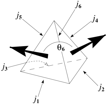
FIG. 1.: A tetrahedral representation of the $6j$-symbol.

FIG. 2.: The isotropic wavefunction $\Psi[B^{3},\{X\}]$ for the range ${0}\leq{X}\leq{200}$.

FIG. 3.: The cutoff expectation value $<l_{X}>$ and uncertainty ${\Delta}l_{X}$ for the isotropic boundary for the range ${0}\leq{K}\leq{200}$.

FIG. 4.: The five distinct two-parameter anisotropic tetrahedra. Edges with length $l_{X}$ are shown in bold, the remaining edges are of length $l_{Y}$.

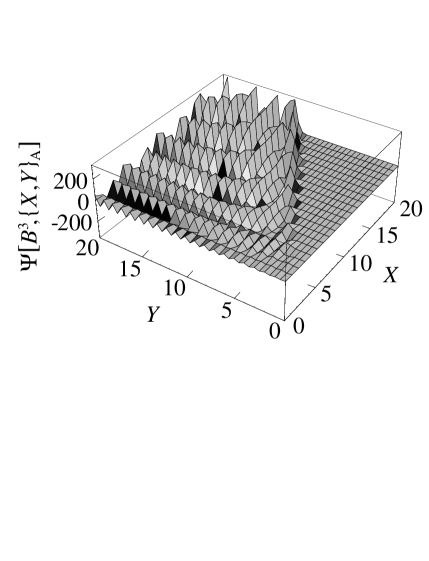
FIG. 5.: The type A wavefunction $\Psi[B^{3},\{X,Y\}_{\rm{A}}]$ as a function of $X$ and $Y$ for ${0}\leq{X}\leq{20}$, ${0}\leq{Y}\leq{20}$. Observe that the wavefunction vanishes where ${{X}\over{Y}}>2$ corresponds to an inadmissible configuration.

FIG. 6.: $<l_{X}>$, ${\Delta}l_{X}$, ${{<{l_{Y}}>}}$ and ${{{\Delta}{l_{Y}}}}$ for the type A tetrahedron for ${0}\leq{K}\leq{200}$.

FIG. 7.: (a) $<l_{X}|_{l_{Y}}>$ and (c) $\Delta l_{X}|_{l_{Y}}$ for the type A tetrahedron as functions of $l_{Y}$ for ${0.5}\leq{l_{Y}}\leq{(K+0.5)}$ for $K$ = 100, 120, 140, 160, 180 and 200; (b) $<l_{X}|_{l_{Y}}>$ and (d) $\Delta l_{X}|_{l_{Y}}$ for the type A tetrahedron as functions of $K$ for ${(l_{Y}-0.5)}\leq{K}\leq{200}$ for $l_{Y}$ = 50.5, 60.5, 70.5, 80.5, 90.5 and 100.5.

FIG. 8.: (a) $<l_{Y}|_{l_{X}}>$ as a function of $l_{X}$ for the type A tetrahedron for ${0.5}\leq{l_{X}}\leq{200.5}$ and $K$ = 200; (b) $<l_{Y}|_{l_{X}}>$ as a function of $K$ for the type A tetrahedron for ${50}\leq{K}\leq{200}$ and $l_{X}$ = 50.5. The expectation values and uncertainties are clearly not linear.

FIG. 9.: (a) $<l_{X}|_{l_{Y}}>$ and (b) $\Delta l_{X}|_{l_{Y}}$ as functions of $l_{Y}$ for the five types of anisotropic tetrahedra for ${0.5}\leq{l_{Y}}\leq{200.5}$ and $K$ = 200.

FIG. 10.: (a) $<l_{Y}|_{l_{X}}>$ and (c) $\Delta l_{Y}|_{l_{X}}$ as functions of $l_{X}$ for the type B and C anisotropic tetrahedra for ${0.5}\leq{l_{X}}\leq{200.5}$ and $K$ = 200; (b) $<l_{Y}|_{l_{X}}>$ and (d) $\Delta l_{Y}|_{l_{X}}$ as functions of $l_{X}$ for the type A, D and E anisotropic tetrahedra for ${0.5}\leq{l_{X}}\leq{200.5}$ and $K$ = 200 are clearly not linear.

REFERENCES

- [1] J. B. Hartle, gr-qc/9701022.
- [2] S. R. Coleman, J. B. Hartle, T. Piran and S. Weinberg, Quantum cosmology and baby universes. Proceedings, 7th Winter School for Theoretical Physics, Jerusalem, Israel, December 27, 1989 - January 4, 1990, (World Scientific, Singapore, 1991).
- [3] J. B. Hartle, gr-qc/9304006.
- [4] M. Gell-Mann and J. B. Hartle, Phys. Rev. D 47, 3345 (1993) [gr-qc/9210010].
- [5] R. B. Griffiths, J. Statist. Phys. 36, 219 (1984).
- [6] R. Omnès, The Interpretation of Quantum Mechanics, (Princeton University Press, Princeton, 1994).
- [7] J. B. Hartle, gr-qc/9404017.
- [8] J. B. Hartle, Phys. Rev. D 49, 6543 (1994) [gr-qc/9309012].
- [9] J. B. Hartle and D. Marolf, Phys. Rev. D 56, 6247 (1997) [gr-qc/9703021].
- [10] J. J. Halliwell, gr-qc/0008046.
- [11] G. Ponzano and T. Regge, in Spectroscopic and Group Theoretical Methods in Physics, edited by F. Bloch, S. G. Cohen, A. De-Shalit, S. Sambursky and I. Talmi (North-Holland, Amsterdam, 1968).
- [12] T. Regge, Nuovo Cim. 19, 558 (1961).
- [13] V. Turaev and O. Viro, Topology 31, 865 (1992).
- [14] H. Ooguri, Nucl. Phys. B 382, 276 (1992) [hep-th/9112072].
- [15] E. Witten, Nucl. Phys. B 311, 46 (1988).
- [16] J. W. Barrett and L. Crane, Class. Quant. Grav. 14, 2113 (1997) [gr-qc/9609030].
- [17] J. B. Hartle and S. W. Hawking, Phys. Rev. D 28, 2960 (1983).
- [18] G. Racah, Physical Review 62, 438 (1942).
- [19] J. W. Barrett and T. J. Foxon, Class. Quant. Grav. 11, 543 (1994) [gr-qc/9310016].
- [20] J. B. Hartle and K. V. Kuchar, in Quantum Theory Of Gravity, edited by S. M. Christensen (Adam Hilger, Bristol, 1984).
- [21] K. Kuchar, in Quantum Gravity 2, edited by C. J. Isham, R. Penrose and D. W. Sciama, (Oxford University Press, New York, 1981).
- [22] V. Moncrief, J. Math. Phys. 30, 2907 (1989).
- [23] A. Hosoya and K. Nakao, Class. Quant. Grav. 7, 163 (1990).
- [24] S. Carlip, Phys. Rev. D 42, 2647 (1990).
- [25] R. Ionicioiu and R. M. Williams, Class. Quant. Grav. 15, 3469 (1998) [gr-qc/9806027].
- [26] E. H. Spanier, Algebraic Topology, (McGraw-Hill, New York, 1966).