Polarized Spacetime Foam

Abstract

An approximate model of a spacetime foam is presented. It is supposed that in the spacetime foam each quantum handle is like to an electric dipole and therefore the spacetime foam is similar to a dielectric. If we neglect of linear sizes of the quantum handle then it can be described with an operator containing a Grassman number and either a scalar or a spinor field. For both fields the Lagrangian is presented. For the scalar field it is the dilaton gravity + electrodynamics and the dilaton field is a dielectric permeability. The spherically symmetric solution in this case give us the screening of a bare electric charge surrounded by a polarized spacetime foam and the energy of the electric field becomes finite one. In the case of the spinor field the spherically symmetric solution give us a ball of the polarized spacetime foam filled with the confined electric field. It is shown that the full energy of the electric field in the ball can be very big.

1 Introduction

One of the manifestation of quantum gravity is a spacetime foam introduced by Wheeler [1] for the description a hypothesized topology fluctuations on the Planck scale level. The spacetime foam is a cloud of appearing/disappearing quantum handles. The appearance/desctruction of these handles leads to the change of spacetime topology. This fact give rise to big difficulties at the description of the spacetime foam since by topology changes of a space (according to Morse theory [2] (Part2, Chap. 2, Sec. 10)) the critical points must exist where the time direction is not defined. In each such point should be a singularity which is an obstacle for the mathematical description of the spacetime foam.

Nevertheless we can try to describe spacetime foam by some approximate manner. For the beginning we offer a model of the single quantum handle as the wormhole-like solution in the Kaluza-Klein gravity. In some approximation we can neglect the linear sizes of the handle and in this case each quantum handle looks as two points pasted together. It is so called a minimalist wormhole [3], i.e. quantum wormhole in which the cross section of the throat is contracted to a point. Afterwards we will introduce an operator which describes the creation/annihilation of the minimalist wormhole. We will show that this operator can be presented as a Grassman number and some (scalar or fermion) field.

It is interesting to compare the model of spacetime foam presented here with another approaches in this field. Now we would like briefly to circumscribe these approaches in the investigations of spacetime foam (for details see review [4]). The spacetime foam and the complicated topological structure connected with it may provide a mechanism for explaining the vanishing of the cosmological constant and for fixing all the constants of nature [5]. The spacetime foam may also induce loss of a quantum coherence [6], and produce a frequency-dependent energy shifts that would slightly alter the dispersion relations for the different low-energy fields [7, 8]. Also spacetime foam has been proposed as a mechanism for regulating both the ultraviolet [9] and the infrared behavior of quantum field theory [10]. The most of these investigations based on the properties of a single or $N$ wormholes forming spacetime foam. Here in the presented model we shall try to describe some effects connected to foam not being interested their internal structure. The difference between this model and above-mentioned approaches is similar to difference between thermodynamics and classical mechanics. The classical mechanics investigates the movement of each single particle in a gas whereas the thermodynamics works with physical quantities which are the average values of microscopical quantities. In the offered model of spacetime foam we are interesting only for cooperative properties of the foam that allows us to introduce some effective field which describes approximately and effectively spacetime foam.

One mouth of quantum wormhole can entrap the electric force lines and then these force lines will emerge from another mouth. It allows us to consider each quantum wormhole as an electric dipole and the spacetime foam as a dielectric [11]. In this case a big electric field can polarize the spacetime foam that can be the reason for some physical effects.

2 The model of a quantum handle

The model of the individual quantum handle is presented on the Fig.(1). It is some realization of the Wheeler idea about a wormhole entrapping electric force lines. In Ref.[1] he wrote: “Along with the fluctuations in the metric there occur fluctuations in the electromagnetic field. In consequence the typical multiply connected space $\ldots$ has a net flux of electric lines of force passing through the ”wormhole”. These lines are trapped by the topology of the space. These lines give the appearance of a positive charge at one end of the wormhole and a negative charge at the other”.

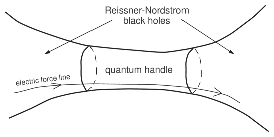
Figure 1: The model of a quantum handle. The whole spacetime is 5 dimensional and: in the Reissner-Nordström black hole $G_{55}=const$ and it is not varying (this is the 5D gravity in the initial Kaluza-Klein interpretation); in the 5D throat $G_{55}$ is the dynamical field.

The composite wormhole on the Fig.(1) consists from two Reissner-Nordström black holes and the 5D throat inserted between them [12]. The 5D metric for this throat is

$$ds^{2}_{(5)}=-R_{0}^{2}e^{2\psi(r)}\Delta(r)\left(d\chi+\omega(r)dt+Q\cos\theta d\varphi\right)^{2}+\frac{1}{\Delta(r)}dt^{2}-dr^{2}-a(r)\left(d\theta^{2}+\sin\theta^{2}d\varphi^{2}\right),$$ (1)

where $\chi$ is the 5^th extra coordinate; $R_{0}$ and $Q$ are some constants. We assume that in some rough approximation the quantum handle in the spacetime foam can be presented by this manner. The 5D Einstein equations for the throat are

$$\frac{\Delta^{\prime\prime}}{\Delta}-\frac{{\Delta^{\prime}}^{2}}{\Delta^{2}}+\frac{\Delta^{\prime}\psi^{\prime}}{\Delta}+\frac{a^{\prime}\Delta^{\prime}}{a\Delta}+R_{0}^{2}{\omega^{\prime}}^{2}\Delta^{2}e^{2\psi} = 0,$$ (2)

$$\omega^{\prime\prime}+\omega^{\prime}\left(2\frac{\Delta^{\prime}}{\Delta}+3\psi^{\prime}+\frac{a^{\prime}}{a}\right) = 0,$$ (3)

$$\frac{a^{\prime\prime}}{a}+\frac{a^{\prime}\psi^{\prime}}{a}-\frac{2}{a}+\frac{Q^{2}\Delta e^{2\psi}}{a^{2}} = 0,$$ (4)

$$\psi^{\prime\prime}+{\psi^{\prime}}^{2}+\frac{a^{\prime}\psi^{\prime}}{a}-\frac{Q^{2}\Delta e^{2\psi}}{2a^{2}} = 0,$$ (5)

$$\frac{{\Delta^{\prime}}^{2}}{\Delta^{2}}+2\frac{\Delta^{\prime}\psi^{\prime}}{\Delta}-4\frac{a^{\prime}\psi^{\prime}}{a}+\frac{4}{a}-\frac{{a^{\prime}}^{2}}{a^{2}}-R_{0}^{2}{\omega^{\prime}}^{2}\Delta^{2}e^{2\psi}-\frac{Q^{2}\Delta e^{2\psi}}{a^{2}} = 0.$$ (6)

It can be shown [13] that there is three type of solutions : the first type (wormhole-like solution) is presented on Fig.(1) with $E>H$ ($E$ and $H$ are Kaluza-Klein electric and magnetic fields), the second one is an infinite flux tube with $E=H$ and the third one is a singular solution (finite flux tube) with $E<H$. The longitudinal size $L_{0}$ of the WH-like solution depends on the relation between electric and magnetic fields : if $(1-H/E)\rightarrow 0$ then $L_{0}\rightarrow\infty$. Now we will describe some properties of the wormhole-like solutions allowing us to interpret their as quantum handles in spacetime foam.

Let us define an approximate solution close to points $r^{2}=r^{2}_{0}$ (where $ds^{2}(\pm r_{0})=0$).

$$\Delta(r) \approx \Delta_{1}\left(r_{0}^{2}-r^{2}\right),$$ (7)

$$\omega(r) \approx \frac{\omega_{1}}{r_{0}^{2}-r^{2}},$$ (8)

$$\psi(r) \approx \frac{\psi_{3}}{6}\left(r_{0}^{2}-r^{2}\right)^{3}.$$ (9)

with

$$\Delta_{1} = \pm\frac{q}{2a_{0}r_{0}},$$ (10)

$$\omega_{1} = \frac{2a_{0}r_{0}}{q},$$ (11)

$$\psi_{3} = \pm\frac{qQ^{2}}{2a_{0}^{3}r_{0}^{3}}$$ (12)

here $a_{0}=a(r=\pm r_{0})$, $q$ is some constant. It is easy to show that at the hypersurfaces $r=\pm r_{0}$ : $ds^{2}=0$. On these hypersurfaces the change of the metric signature takes place : $(+,-,-,-,-)$ by $|r|<r_{0}$ and $(-,-,-,-,+)$ by $|r|>r_{0}$. Following to Bronnikov [15] we call these two hypersurfaces as $T-$horizons.

For the definition of a Kaluza-Klein electric field we consider Eq.(3)

$$\left[\left(\omega^{\prime}\Delta^{2}e^{3\psi}\right)4\pi a\right]^{\prime}=0$$ (13)

here $4\pi a$ is the area of $S^{2}$ sphere. Comparing with the Gauss law we see that Kaluza-Klein electric field $E_{KK}$ can be defined as follows

$$E_{KK}=\omega^{\prime}\Delta^{2}e^{3\psi}=\frac{q}{a}$$ (14)

here $q$ is an electric charge which is proportional to a flux of electric field. In this case the force lines of the electric field are uninterrupted and can be continued through the surfaces of matching the 5D WH-like solution and the Reissner-Nordström solution like to Fig.1.

On these $T-$horizons we should match:

• the flux of the 4D electric field (defined by the 4D Maxwell equations) with the flux of the 5D electric field defined by $R_{5t}=0$ Kaluza-Klein equation.

• the area of the Reissner-Nordström event horizon with the area of the $T-$horizon.

In the spacetime foam can be two different types of quantum handles : the first type does not entrap the electric force lines, the second type respectively entrap these lines. We will not consider the first type of quantum handles. In this case the quantum handle of the second type (in the minimalist wormhole approximation) is presented on Fig. 2.

In the next section we will consider an approximate model of the spacetime foam where we neglect the cross section of quantum handles. It means that the area of cross section of the throat is contracted into a point. Such approximation for the quantum handle is called as the minimalist wormhole. And further we will consider the consequences for such approximation. Thus, in this section we have presented a microscopic model of the quantum handle. But in the next sections we will consider an effective model of the spacetime foam where we will neglect of the cross section of quantum handles in the spacetime foam.

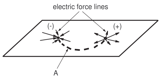
Figure 2: The minimalist wormhole as a quantum handle in the spacetime foam. One mouth entraps and another one emits the electric force lines and looks as two connected points. The curve A schematically shows the identification of these two points

3 The operator description of the minimalist wormhole

Let us introduce an operator $W(x,y)$ which describes creation/annihilation minimalist wormhole connected two points $x$ and $y$ [3] [16]. Let the operator $W(x,y)$ has the following property

$$W^{2}(x,y)=0.$$ (15)

It means that the reiterated creation/annihilation minimalist wormhole is senseless. This property tell us that the operator $W(x,y)$ can be connected with the Grassman numbers. In the general case the operator $W(x,y)$ is nonlocal one but in this paper we will consider the simplest case when $W(x,y)$ can be factorized on two local operators

$$W(x,y)=\theta(x)\theta(y).$$ (16)

The operator $\theta(x)$ can be considered as a readiness of a point $x$ to pasting together with a point $y$ (or conversely the separation these points in the minimalist wormhole).

We will consider three cases.

The first case is

$$W^{ab}(x,y)=\phi(x)\theta^{a}\phi(y)\theta^{b}$$ (17)

where $a,b$ are the undotted spinor indices, $\phi(x)$ is the scalar field, $\theta^{a}$ is the Grassman number

$$\theta^{a}\theta^{b}+\theta^{b}\theta^{a}=0.$$ (18)

It is easy to proof that

$$W^{ab}(x,y)W_{ab}(x,y)=\phi^{2}(x)\phi^{2}(y)\theta^{a}\theta^{b}\theta_{a}\theta_{b}=\phi^{2}(x)\phi^{2}(y)\varepsilon_{aa^{\prime}}\varepsilon_{bb^{\prime}}\theta^{a}\theta^{b}\theta^{a^{\prime}}\theta^{b^{\prime}}\equiv 0$$ (19)

where

$$\varepsilon^{ab}=\begin{pmatrix}0&1\\ -1&0\end{pmatrix},\qquad\varepsilon_{ab}=\begin{pmatrix}0&-1\\ 1&0\end{pmatrix}.$$ (20)

Eq. 19 means that it makes no sense to identify two points twice.

The second case is

$$W(x,y)=\psi_{a}(x)\theta^{a}\psi_{b}(y)\theta^{b}=\psi_{a}(x)\psi_{b}(y)\theta^{a}\theta^{b}=\left(\psi_{1}(x)\psi_{2}(y)-\psi_{2}(x)\psi_{1}(y)\right)\theta^{1}\theta^{2}$$ (21)

where $\psi_{a}(x)$ is an undotted spinor field in $(\frac{1}{2},0)$ representation. The square is zero

$$W^{2}(x,y)=\left(\psi_{1}(x)\psi_{2}(y)-\psi_{2}(x)\psi_{1}(y)\right)^{2}\theta^{1}\theta^{2}\theta^{1}\theta^{2}\equiv 0.$$ (22)

In this case $W(x,x)\equiv 0$. It means that the minimalist wormhole can connect only two different points.

The third case is

$$W(x,y)=\psi_{a}(x)\theta^{a}\psi_{\dot{b}}(y)\bar{\theta}^{\dot{b}}=\psi_{a}(x)\psi_{\dot{b}}(y)\theta^{a}\bar{\theta}^{\dot{b}}$$ (23)

where $\psi_{\dot{b}}$ is a dotted spinor in $(0,\frac{1}{2})$ representation. The square is zero

$$W^{2}(x,y)=\left(\psi_{a}(x)\psi_{\dot{b}}(y)\theta^{a}\bar{\theta}^{\dot{b}}\right)\left(\psi_{c}(x)\psi_{\dot{d}}(y)\theta^{c}\bar{\theta}^{\dot{d}}\right)=\Bigl{(}\psi_{a}(x)\psi_{c}(x)\theta^{a}\theta^{c}\Bigr{)}\left(\psi_{\dot{b}}(y)\psi_{\dot{d}}(y)\bar{\theta}^{\dot{b}}\bar{\theta}^{\dot{d}}\right)\equiv 0$$ (24)

as

$$\psi_{a}(x)\psi_{c}(x)\theta^{a}\theta^{c}=\psi_{1}(x)\psi_{2}(x)\theta^{1}\theta^{2}+\psi_{2}(x)\psi_{1}(x)\theta^{2}\theta^{1}\equiv 0.$$ (25)

We must note that as the classical canonical theory cannot describes topology change these operators do not correspond to any classical observables. It corresponds to the well-known fact that the Grassman numbers do not have any classical interpretation.

We can suppose that $W(x,y)$ operator is described with dynamical fields : scalar field $\phi(x)$ or spinor field $\psi(x)$. Below we will present some equations for these fields and discuss the physical sense of corresponding solutions.

It is interesting to note that in Ref. [7] very similar idea is considered that the gravitational interactions (topology fluctuations) presented in the spacetime foam are modelled by means of nonlocal interactions (operator $W(x,y)$ in our case) that relate spacetime points and these nonlocal interactions can be described in terms of local interactions ($\theta(x)$ in our case).

The operator $W(x,y)$ can be connected with an indefiniteness (the loss of information) of our knowledge about two points $x^{\mu}$ and $y^{\mu}$ : we do not know if these points are connected by the quantum minimalist wormhole or not. We would like to note that the similar idea was considered in Ref. [14] : the author investigates the consequences of the loss of information about the topology of the background spacetime and found that the existence of spacetime foam leads to a situation where the number of bosonic fields is a variable quantity.

Are the functions $\phi(x)$ and $\psi(a(x)$ dynamical or not ? Of coarse, in the context of this paper we do not have the answer on this question because here is proposed only an effective model of the spacetime foam. The exact model of the spacetime foam can be obtained only from a quantum gravity theory. From the physical point of view we can expect that the state and properties of spacetime foam depend on the magnitude of gravitational and external (for example, E&M) fields. The aim of this paper is to try to describe the state of spacetime foam by some effective way using some (scalar/spinor) field. Common sense guides us to suppose that it is possible if we neglect the cross section of each quantum handle in the spacetime foam. It means that each quantum handle looks like to two points connected by a line (see, Fig. 2) and this (scalar or spinor) field give us an information about quantum handles. Below we will see that it is the information about the typical length of quantum handles in the spacetime foam.

Another question appearing in the context of this section is : what kind of wormhole operator is realized in the real spacetime foam or every such possibility can happen in the spacetime foam ? Again the answer lies in quantum gravity theory. Nevertheless, we can compare the results of similar calculations for the different choice of the minimalist operator in order that to select those coincides with our common sense. For this we will compare the wormhole operator $W(x,y)$ for the different cases : for the scalar and spinor fields. It is evident that $W(x,y)\approx 0$ if the points $x$ and $y$ are well away from each other. For example, for the ordinary spacetime foam (without any external influence)

$$W(x,y)\approx 0\quad\text{for}\quad|x-y|>l_{Pl}.$$ (26)

Consequently we will use this criteria in the next sections for the choice between all possibilities for the effective field (scalar or spinor).

4 The scalar field

For the description of the dynamics of the scalar field we offer the following (dilaton gravity + Maxwell) Lagrangian

$${\cal L}=-\sqrt{-g}\left(R+2\nabla_{\mu}\phi\nabla^{\mu}\phi-e^{-2\phi}F_{\mu\nu}F^{\mu\nu}\right)$$ (27)

where $g$ is the determinant of the 4D metric, $R$ is the Ricci scalar, $\phi$ is the dilaton field and $F_{\mu\nu}=\partial_{\mu}A_{\nu}-\partial_{\nu}A_{\mu}$ is the tensor of the electromagnetic field, $\mu=0,1,2,3$. It means that we interpret the above-mentioned scalar field as the dilaton field. The corresponding field equations are

$$\nabla_{\nu}\left(e^{-2\phi}F^{\mu\nu}\right) = 0,$$ (28)

$$\nabla_{\mu}\nabla^{\mu}\phi = \frac{1}{2}e^{-2\phi}F_{\mu\nu}F^{\mu\nu},$$ (29)

$$R_{\mu\nu}-\frac{1}{2}R = \varkappa T_{\mu\nu}$$ (30)

where $R_{\mu\nu}$ is the Ricci tensor and $T_{\mu\nu}$ is the tensor-momentum for dilaton and Maxwell fields. Each minimalist wormhole (as a quantum handle in the spacetime foam) looks as a dipole because one mouth entraps the electric force lines and another mouth will emerges these force lines. At first sight our choice of scalar field as the dilaton field is arbitrary but now we would like to explain why it is the natural choice. If we take a look over Fig.2 than we see that the electric force lines around the quantum handle behave like to electric force lines in the presence of an electric dipole. How we can effectively (and approximately) describe the set of minimalist wormholes which entrap and emerge electric force lines ? We suppose that an external electric field acts on the minimalist wormhole (quantum handle) so that they line up with the electric field. Then such orientation of the minimalist wormholes will change the external electric field just as it happens in a dielectric. Another words we can introduce an effective electric displacement $\vec{D}$ which will describe the result of polarization of spacetime foam. As usually this vector $\vec{D}$ should be connected with the electric field as $\vec{D}=\varepsilon\vec{E}$ (where $\varepsilon$ is a dielectric permeability). The ordinary Maxwell equations looks as

$$\partial_{\nu}\left(\varepsilon F^{\mu\nu}\right)=0.$$ (31)

Comparing Eq. (31) with the Maxwell + dilaton equation Eq. (28) we see that the dielectric permeability $\varepsilon$ can be connected with the dilaton field $\phi$ by the following way

$$\varepsilon=e^{-2\phi}$$ (32)

and the electric displacement $\vec{D}$

$$\vec{D}=\varepsilon\vec{E}=e^{-2\phi}\vec{E}=\vec{E}+\vec{P}=\left(1+4\pi\chi\right)\vec{E}$$ (33)

where $\vec{P}$ is the polarization vector.

We would like to consider the static spherically symmetric case with the metric

$$ds^{2} = A^{2}(r)dt^{2}-\frac{dr^{2}}{A^{2}(r)}-\rho^{2}(r)\left(d\theta^{2}+\sin^{2}\theta d\varphi^{2}\right),$$ (34)

$$F_{tr} = E_{r}\neq 0.$$ (35)

The solution is [17]

$$A^{2}(r) = 1-\frac{r_{+}}{r},$$ (36)

$$\rho^{2}(r) = r(r-2r_{0}),$$ (37)

$$e^{2\phi(r)} = \frac{\rho^{2}}{r^{2}}=1-\frac{2r_{0}}{r},$$ (38)

$$E_{r}(r) = \frac{Q}{r^{2}},$$ (39)

$$D_{r}(r) = \frac{Q}{\rho^{2}},$$ (40)

$$r_{0} = \frac{Q^{2}}{r_{+}}$$ (41)

where $r_{+}$ and $r_{0}$ are some constants, $Q$ is the electric charge. For us interesting is the following case

$$r_{0}\gg r_{+}\qquad\text{or}\qquad r_{+}\ll Q$$ (42)

where the electric charge and field is in the natural units : $[Q]=cm$ and $[E]=cm^{-1}$. It is necessary to note that we have a gravitational singularity at the point $r=2r_{0}$ ($\rho=0$).

Our interpretation of this solution is the following. It is a bare electric charge $Q$ surrounded by a polarized spacetime foam (PSF). The PSF is described by the dilaton field $\phi$ which is connected with the operator $W(x,y)$ describing the minimalist wormhole (17). At the infinity $\phi(r)=0$ that means $W(x,y)=0$ and $\varepsilon=e^{-2\phi}=1$, i.e. the PSF absents at the infinity. Let us consider

$$W^{ab}(\vec{x},\vec{y})=\frac{1}{4}\ln\left(1-\frac{2r_{0}}{\left|\vec{x}-\vec{x_{0}}\right|}\right)\left(1-\frac{2r_{0}}{\left|\vec{y}-\vec{y_{0}}\right|}\right)\theta^{a}\theta^{b}\quad r\geq 2r_{0}$$ (43)

where $\phi(\vec{x})=\phi(|\vec{x}-\vec{x_{0}}|)$; $\vec{x}_{0}$ and $\vec{y}_{0}$ are the locations of the mouthes of the minimalist wormhole (quantum handle). We see that $W^{ab}(\vec{x},\vec{y})\approx 0$ by $|\vec{x}_{0}-\vec{y}_{0}|\gg 2r_{0}$. It allows us to say that in the spacetime foam only the points on the distance $l\approx r_{0}$ can be pasted together making the quantum handle. In such interpretation $r_{0}\approx l_{Pl}$. Nevertheless, in some external field the magnitude $r_{0}$ can have various values. As it was mentioned in Sec. 2 the longitudinal size of the solution presented there can have arbitrary value which depends on the relation between electric $E$ and magnetic $H$ fields. It means that in the presence of a big external magnetic field the magnitude $r_{0}$ can be very large.

Now we would like to present some physical consequences of our model of the bare charge imbedded in the PSF.

4.1 The screening of the bare charge

In this subsection we would like to calculate a surface density of bounded electric charges connected with the polarization of the spacetime foam. At first we will calculate the normal component $P_{n}=P_{r}$ of the polarization vector

$$4\pi P_{r}=D_{r}-E_{r}=Q\left(\frac{1}{\rho^{2}}-\frac{1}{r^{2}}\right).$$ (44)

The surface density $\sigma$ of the bound charges is

$$\sigma=P_{n}=P_{r}.$$ (45)

Consequently a charge $Q_{anti}$ on the little sphere surrounding the bare charge $Q$ is

$$Q_{anti}=-\left|4\pi\rho^{2}\sigma\right|=-Q\left(1-\frac{\rho^{2}}{r^{2}}\right)=-Q\frac{2r_{0}}{r}\xrightarrow{r\rightarrow 2r_{0}}-Q.$$ (46)

Thus the PSF completely shield the bare electric charge. Another consequence is that the PSF intercepts all the force lines of the bare charge and redistributes their in the surrounding space.

4.2 The energy of the shielded charge

From the above-mentioned results we see that the spacetime foam surrounding the bare electric charge redistributes electric force lines by such a way that the charge is screened. This leads to the fact that the effective electric displacement can be introduced and as the consequence the energy density of the bare charge is changed. In this subsection we would like to calculate the energy of the electric charge surrounded by the PSF. Let us calculate the energy $W$ of the electric field

$$W=\frac{1}{8\pi}\int_{2r_{0}}^{\infty}D_{r}E_{r}\sqrt{-\gamma}dr\approx\frac{Q^{2}}{4r_{0}}$$ (47)

where we have used the condition $r_{+}\ll r_{0}$ and $\gamma$ is the determinant of the 3D metric. Eq. (47) is very interesting. We see that the energy of the charge surrounded by the PSF depends on some characteristic length $r_{0}$ which is connected with the typical length of quantum handles in spacetime foam. Usually the typical length of quantum handles is $l_{Pl}$. In this case $W\approx Q^{2}/l^{2}_{Pl}$ and the advantage of this formula is evident : it is a finite number whereas the energy of the point charge in the classical electrodynamics is infinite number.

As indicated above there is the possibility when the typical length of quantum handles can be larger (in the presence of a big external magnetic field). It is interesting to determine the value of $r_{0}$ so that this energy can be compared with the rest energy of electron

$$m_{0}c^{2}=\frac{e^{2}}{4r_{0}},\qquad Q=e$$ (48)

where $m_{0}$ is the rest mass of electron. In this case the typical length of quantum handles is $r_{0}\approx 10^{-13}cm$ ($r_{+}\approx 10^{-45}$) and it can be compared with the classical radius of electron. Of coarse such value of quantum handles is too much.

4.3 The gravitational effects

Now we would like to calculate some gravitational effects connected with the metric (34). The metric approximately is

$$ds^{2}\approx dt^{2}-dr^{2}-r(r-2r_{0})\left(d\theta^{2}+\sin^{2}\theta d\varphi^{2}\right),\quad r\geq 2r_{0}.$$ (49)

We see that the metric in this model is not flat. The difference can be measured as a deficit of the sphere area

$$\delta=1-\frac{4\pi l^{2}_{\rho}}{4\pi\rho^{2}}$$ (50)

where $l_{\rho}$ is the distance between the origin ($r=2r_{0}$) and the sphere with the radius $\rho=\sqrt{r(r-2r_{0})}$

$$l_{\rho}=\int_{2r_{0}}^{r}\frac{dr}{\sqrt{1-\frac{r_{+}}{r}}}\approx\left(r-2r_{0}\right).$$ (51)

It means that

$$\delta\approx 1-\frac{\left(r-2r_{0}\right)^{2}}{\rho^{2}}=\frac{2}{3}\qquad\text{by}\qquad r=3r_{0}.$$ (52)

Let us remind that in the chosen coordinate system $r>2r_{0}$ .

Thus this model of electron with the PSF give us the finite rest energy of electron (connected with its renormalized electric field) but at the center of electron we have a gravitational singularity. Also we should note that at the center of electron the electric field $E_{r}=\frac{Q}{2r_{0}}$ is finite but the direction of this vector is undefined. The picture of $\vec{E}$ at the center is like to a hedgehog.

The experimental verified consequences of this model is the nonflat metric (49) and the difference between $D_{r}$ and $E_{r}$. For example, at the distance $r-2r_{0}\approx r_{0}$ we have the deficit of the sphere area

$$\delta\approx\frac{2}{3}$$ (53)

and the dielectric permeability

$$\varepsilon=\frac{D_{r}}{E_{r}}=\frac{r^{2}}{\rho^{2}}=\frac{1}{1-\frac{2r_{0}}{r}}\approx 3.$$ (54)

Evidently it is too much but it can be connected with that our dilaton model of the PSF is approximate one. Nevertheless on the basis of such model we have the interesting model of screening of the bare electric charge with the finite energy of the electric field.

5 The spinor field

In this section we would like to consider the spinor model of the PSF with the following Lagrangian

$${\mathcal{L}}=\sqrt{-g}\left\{-\frac{1}{2k}\left(R+\frac{1}{4}\mathcal{F}_{\alpha\beta}\mathcal{F}^{\alpha\beta}\right)+\right.$$

$$\left.\frac{\hbar c}{2}\left[i\bar{\psi}\left(\gamma^{\mu}\nabla_{\mu}-\frac{1}{8}\mathcal{F}_{\alpha\beta}\gamma^{[\alpha}\gamma^{\beta]}-\frac{1}{4}l^{2}_{0}\left(\gamma^{5}\gamma^{\mu}\right)\left(i\bar{\psi}\gamma^{5}\gamma_{\mu}\psi\right)-\frac{m}{i}\right)\psi+h.c.\right]\right\}$$ (55)

where $\mathcal{F}_{\alpha\beta}=\frac{c^{2}}{k}F_{\alpha\beta}$; $\mathcal{F}_{\alpha\beta}$ and $F_{\alpha\beta}$ are the Maxwell tensor in the natural and CGS units respectively; $\alpha,\beta,\mu$ are the 4D world indexes, $\gamma^{\mu}$ are the 4D $\gamma$ matrixes with usual definitions $\gamma^{\mu}\gamma^{\nu}+\gamma^{\nu}\gamma^{\mu}=2\eta^{\mu\nu}$, $\eta^{\mu\nu}=(+,-,-,-)$ is the signature of the 4D metric; $l_{0}$ is some length; $k=6.67\times 10^{-8}cm^{3}g^{-1}s^{-2}$ is the gravitational constant. Of coarse Lagrangian (55) is an arbitrary choice of a “fermion-generated” spacetime foam model. Nevertheless there are some arguments for the nonminimal $(\bar{\psi}\mathcal{F}_{\alpha\beta}\gamma^{\alpha}\gamma^{\beta}\psi)$ and nonlinear $(\bar{\psi}\gamma^{5}\gamma^{\mu}\psi)(\bar{\psi}\gamma^{5}\gamma_{\mu}\psi)$ terms. These terms have the natural origin in the 5D gravitational Lagrangian with a torsion after the 4D dimensional reduction. Our hope is that the future investigations will give us the more natural explanation for this choice. Varying with respect to $g_{\mu\nu}$, $\bar{\psi}$ and $A_{\mu}$ leads to the following equations

$$R_{\mu\nu}-\frac{1}{2}g_{\mu\nu}R = \varkappa T_{\mu\nu},$$ (56)

$$D_{\nu}\mathcal{H}^{\mu\nu} = 0,\,$$ (57)

$$\left[i\gamma^{\mu}\nabla_{\mu}-\frac{1}{8}\mathcal{F}_{\alpha\beta}\left(i\gamma^{[\alpha}\gamma^{\beta]}\right)-\frac{1}{2}l^{2}_{0}\left(i\gamma^{5}\gamma^{\mu}\right)\left(i\bar{\psi}\gamma^{5}\gamma_{\mu}\right)-m\right]\psi = 0,$$ (58)

$$\mathcal{H}^{\mu\nu} = \mathcal{F}^{\mu\nu}+f^{\mu\nu},$$ (59)

$$f^{\mu\nu} = 4l^{2}_{0}\left(i\bar{\psi}\gamma^{[\mu}\gamma^{\nu]}\psi\right)$$ (60)

where $\nabla_{\mu}=\partial_{\mu}-\frac{1}{4}\omega_{ab\mu}\gamma^{[a}\gamma^{b]}$ is the 4D covariant derivative of the spinor field, $\omega_{ab\mu}$ is the 4D Ricci coefficients, $a,b$ are the fier-bein indices, $f_{\mu\nu}$ is the polarization tensor of the spacetime foam, $[]$ means the antisymmetrization. This equation set is very complicated therefore we will consider here only the PSF + electrodynamics, i.e. gravity will be excluded.

Let us consider the case when we do not have the external electrical charges. It allows us to resolve the Maxwell equation (57)

$$\mathcal{F}_{\mu\nu}=-f_{\mu\nu}=-4l_{0}^{2}\left(i\bar{\psi}\gamma_{[\mu}\gamma_{\nu]}\psi\right).$$ (61)

Then the Dirac equation has the following form

$$\left\{i\gamma^{\mu}\nabla_{\mu}+\frac{l_{0}^{2}}{2}\left[\left(i\gamma^{[\mu}\gamma^{\nu]}\right)\left(i\bar{\psi}\gamma_{[\mu}\gamma_{\nu]}\psi\right)-\left(i\gamma^{5}\gamma^{\mu}\right)\left(i\bar{\psi}\gamma^{5}\gamma_{\mu}\psi\right)\right]-m\right\}\psi=0.$$ (62)

Immediately we see that it is one of variants of the non-linear Heisenberg equations (the Dirac equation + a non-linear term). The solution we will search in the following form

$$\psi(r,\theta,\varphi)=e^{i\omega t}\begin{pmatrix}f(r)\\ 0\\ ig(r)\cos\theta\\ ig(r)\sin\theta e^{i\varphi}\end{pmatrix}.$$ (63)

After substitution in Eq. (62) we have

$$g^{\prime}+\frac{2}{r}g+f(m+\omega)-l_{0}^{2}f\left(f^{2}-g^{2}\right) = 0,$$ (64)

$$f^{\prime}+g\left(m-\omega\right)-l_{0}^{2}g\left(f^{2}-g^{2}\right) = 0.$$ (65)

In the Ref. [18] it is shown that such equations set has regular solutions. At the origin $r=0$ this solution can be expanded into a series

$$f(r) = f_{0}+\frac{f_{2}}{2}r^{2}+\ldots,$$ (66)

$$g(r) = g_{1}r+\frac{g_{3}}{3!}r^{3}+\ldots$$ (67)

with

$$g_{1} = \frac{1}{3}f_{*}\left[l_{0}^{2}f_{*}^{2}-\left(m+\omega\right)\right],$$ (68)

$$f_{2} = g_{1}\left[l_{0}^{2}f_{*}^{2}-\left(m-\omega\right)\right]$$ (69)

where $f_{*}$ is a value of $f_{0}$ for which there is the above-mentioned regular solution for $f(r)$ and $g(r)$, i.e. for the another $f_{0}\neq f_{*}$ the solution has an infinite energy.

The asymptotical behavior of the regular solution is

$$f(r) = \frac{\tilde{f}}{l_{0}\sqrt{m}}\frac{e^{-r\sqrt{m^{2}-\omega^{2}}}}{r}+\ldots,$$ (70)

$$g(r) = \frac{\tilde{f}}{l_{0}\sqrt{m}}\sqrt{\frac{m+\omega}{m-\omega}}\frac{e^{-r\sqrt{m^{2}-\omega^{2}}}}{r}+\ldots\qquad.$$ (71)

where $\tilde{f}$ is some constant. Let us come back to the Maxwell fields. For our spinor ansatz we have the following components of the electric and magnetic fields

$$\mathcal{E}^{r}(r) = -f^{tr}(r)=8l_{0}^{2}f(r)g(r),$$ (72)

$$\mathcal{H}_{\theta}(r) = \frac{1}{2}\epsilon_{\theta r\varphi}f^{r\varphi}(r)=4l_{0}^{2}\sin\theta\Bigl{(}f^{2}(r)+g^{2}(r)\Bigr{)},$$ (73)

$$\mathcal{H}_{r}(r) = \frac{1}{2}\epsilon_{r\theta\varphi}\sqrt{-\gamma}f^{\theta\varphi}(r)=4l_{0}^{2}\cos\theta\Bigl{(}g^{2}(r)-f^{2}(r)\Bigr{)}$$ (74)

here $\mathcal{E}_{i}$ and $\mathcal{H}_{i}$ are the electric and magnetic fields in the natural units. The corresponding magnitudes in the CGS units are $E_{i}=\frac{\sqrt{k}}{c^{2}}\mathcal{E}_{i}$ and $H_{i}=\frac{\sqrt{k}}{c^{2}}\mathcal{H}_{i}$. Now we have to do the following important simplifying remark. The ansatz for the spinor field (63) has a preferred direction (the spin direction) but the PSF is a quantum fluctuating object therefore we should average our results over the spin direction. It means that we should average electric and magnetic fields over $\theta$ ($0\leq\theta\leq 2\pi$) that give us

$$\mathcal{H}_{\theta} = \mathcal{H}_{r}=0,$$ (75)

$$\mathcal{E}_{r} = 8l_{0}^{2}f(r)g(r).$$ (76)

Now we are ready to formulate the result. Our solution with $\psi$ and $\mathcal{E}_{r}$ describes a ball of the polarized spacetime foam filled with the electric field. Another words, the PSF can confine electric field in some volume and it is a pure quantum gravity phenomenon. We can expect that the energy density of the electric field will be very big and it will depend on the properties of the PSF, i.e. on the typical length of quantum handles.

Eq’s (70) - (71) show us that the spinor field is nonzero inside of a region with the linear sizes $\approx r_{0}=(m^{2}-\omega^{2})^{-1/2}$. It means that the operator $W(x,y)$ is nonzero in this region and consequently the typical length of quantum handles are $r_{0}$.

5.1 The energy of the PSF ball

The basic purpose of this section is to calculate the PSF ball with the confined electric field and compare this energy with some big interesting energies (nuclear bomb, Gamma Ray Burst (GRB)). At first we would like to write Eq’s (64) (65) in the dimensionless form

$$\bar{g}^{\prime}+\frac{2}{x}\bar{g}+\bar{f}(1-\beta)-\bar{f}\left({\bar{f}}^{2}-{\bar{g}}^{2}\right) = 0,$$ (77)

$$\bar{f}^{\prime}+\bar{g}(1+\beta)-\bar{g}\left({\bar{f}}^{2}-{\bar{g}^{2}}\right) = 0,$$ (78)

$$\bar{f}(x)=\frac{l_{0}}{\sqrt{m}}f(r),\qquad\bar{g}(x)=\frac{l_{0}}{\sqrt{m}}g(r),\qquad x=rm,\qquad\beta = -\frac{\omega}{m}.$$ (79)

The numerical solution of these equations presented on the Fig.3.

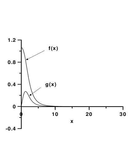
Figure 3: The functions $\bar{f}(x)$ and $\bar{g}(x)$. $\beta=0.9$, $f_{*}\approx 1.06477126$.

And now we can calculate the energy of the electric field

$$W=\frac{1}{8\pi}\frac{c^{4}}{k}\int_{0}^{\infty}\mathcal{E}_{r}^{2}4\pi r^{2}dr=32\frac{c^{4}}{k}\frac{1}{m}\int_{0}^{\infty}\bar{f}^{2}(x)\bar{g}^{2}(x)x^{2}dx$$ (80)

where the numerical coefficient $\frac{c^{4}}{k}$ is necessary for the conversion the natural units to the CGS units. The numerical value of the integral is of the order of 1. Therefore we can estimate the value of $m$

$$32\frac{c^{4}}{k}\frac{1}{m}\approx W\quad\text{and}\quad m\approx 32\frac{c^{4}}{k}\frac{1}{W}$$ (81)

Now we would like to calculate the radius $r_{0}$ and electric field $E$ for two characteristic energies.

1. Nuclear bomb. In this case $W\approx 10^{20}erg$ and

$$m\approx 4\times 10^{30}cm^{-1}\qquad\text{and}\qquad r_{0}\approx\frac{1}{\sqrt{m^{2}-\omega^{2}}}=\frac{1}{m\sqrt{1-\beta^{2}}}\approx 0.6\times 10^{-30}cm$$ (82)

The value of the electric field can be estimated as

$$E_{r}=\frac{c^{2}}{\sqrt{k}}8l_{0}^{2}fg=\frac{c^{2}}{\sqrt{k}}m\bar{f}\bar{g}\approx 256\frac{c^{6}}{k^{3/2}}\frac{1}{W}$$ (83)

The values of the $\bar{f}$ and $\bar{g}$ inside of the ball are of the order of unity. It gives us

$$E_{r}\approx 10^{56}CGS$$ (84)

Consequently the PSF ball filled with the electric field can contain the energy of the order of the energy of the nuclear bomb. It can happen if the typical length of the quantum handles is $\approx 10^{-30}cm$.

1. Gamma Ray Burst. In this case $W\approx 10^{53}erg$ and

$$m\approx 4\times 10^{-3}cm^{-1}\qquad\text{and}\qquad r_{0}\approx\frac{1}{\sqrt{m^{2}-\omega^{2}}}\approx 0.5\times 10^{3}cm=5.00m$$ (85)

The electric field is estimated as

$$E_{r}\approx 10^{23}CGS.$$ (86)

Consequently the PSF ball filled with the electric field can contain the energy of the order of the energy of the GRB and the linear sizes of this ball are of the order of $\approx 10m$. It means that : in order to obtain such energy $W\approx 10^{53}erg$ the typical length of quantum handles must be $r_{0}\approx 10m$. Again we would like remind that there is a possibility to make handles with the big longitudinal size : it can be in the presence of the big external magnetic field. In conclusion we would like to say that the big E&M fields can produce quantum gravitational effects with the release of enormous amount of energy.

The value of such energies latent in the PSF ball is not surprising because it is quantum gravity effects. The big question here is : can be such energy of the electric field extracted from the frozen state in the polarized spacetime foam ? Another questions are : how can be such objects created and how fast it will disintegrate ? Another interesting peculiarity of the spinor equation is that $l_{0}$ can be the Planck length $l_{0}=l_{Pl}$ and nevertheless this microscopical equation can give the macroscopical energy and linear sizes !

5.2 Non-linear Heisenberg equation

It is interesting to note that Eq. (62) is one of the variants of the Heisenberg equation for a non-linear spinor field [19]. This remark allows us to take a new interpretation of the solutions obtained in these Ref’s : it is the PSF ball on a microscopical level.

6 Conclusions

In this paper we offer an approximate model of the polarized spacetime foam. The microscopically description is based on the operator $W(x,y)$ of creation/destruction the minimalist wormholes. The minimalist wormhole is some approximation for the quantum handle when it is contracted into a point. The model for the quantum handle is given by the wormhole-like solution of the 5D Kaluza-Klein gravity. This metric contains off-diagonal components of the 5D metric $G_{5t}$ and $G_{5\varphi}$ which can be considered as an electric and magnetic fields. It allows us to consider each quantum handle (minimalist wormhole) as an electric dipole. Obviously that in such point of view the spacetime foam can be polarized in the presence of an external electric field.

The operator $W(x,y)$ can be connected with either a scalar or a spinor field. Here the question arises : is this operator a consequence of quantum gravity or it is an additional stuff in quantum gravity describing the topology changes ? We assume that these fields can be dynamical. As a model of the scalar field we propose the dilaton field. In this case the dilaton field describes a polarization of the spacetime foam. In the result we have a shielding of the bare electric charge and the finiteness of the energy of the electric field. The physical sense of the scalar/spinor fields in the operator $W(x,y)$ is the following : the product $\varphi(x)\varphi(y)$ (or $\psi_{\alpha}(x)\psi_{\beta}(y)$) describes the typical length of quantum handles in the spacetime foam, i.e. the linear sizes of the region where this product is nonzero characterizes the typical length of quantum handles.

In the another variant a spinor field describes the polarization of the spacetime foam. We have considered the simplest case without external electric charges and gravity. We have shown that the polarized spacetime foam can confine an electric field in some finite region of the space. The magnitude of the confined electric field can be very big. We have shown that this energy depends on the typical length of quantum handles and for the energy of nuclear bomb this length is $r_{0}\approx 10^{-30}cm$ and for the GRB it is $r_{0}\approx 10m$. It is necessary to note that in the consequences of the very high energy density of the electric field confined in the PSF the experimental verification of the effects connected with quantum gravity is very dangerous, much more dangerous then the experiments with the nuclear energies !

In this paper we have considered two possibilities for the description of the spacetime foam : the scalar and spinor fields. Of coarse, the choice between these two possibilities can be made either on the basis of an exact theory of quantum gravity or from an experiment. Unfortunately, we do not have neither. Therefore we can only compare the consequences of two approaches and choose more natural. The comparison of solutions for the scalar field Eq’s (36) - (40) and spinor field Fig. 3 shows us that the first solution has a singularity at the center of the field whereas the spinor field does not have a singularity. It means that the spinor field is more natural choice for the description of the PSF. Another argument for this statement is the following. Let us compare the polarization vector for the “scalar-generated” model of the spacetime foam

$$\mathcal{P}_{i}=\left(e^{-2\phi}-1\right)E_{i}$$ (87)

and for the “fermion-generated” model of the spacetime foam

$$\mathcal{P}^{i}=f^{ti}=4l_{0}^{2}\left(i\bar{\psi}\gamma^{[t}\gamma^{i]}\psi\right)$$ (88)

Now we see how is the difference between the “scalar-generated” and “fermion-generated” models of the spacetime foam. For the first case the polarization vector (87) is proportional to an external electric field $E_{i}$ whereas in the second case $\mathcal{P}_{i}$ does not direct depend on this field. The second case is more interesting since in this case we have very intriguing situation : an electric field can be confined with the spacetime foam in some finite region without any hairs at the infinity. In fact such situation was discussed in Sec.5. It is very unusual situation when a static electric field exists without any electric charges. The explanation for this fact is very simple : the sum of this electric field and the electric field generated by spacetime foam is zero (see, Eq. (61)).

Finally we would like to summarize

• Each quantum handle in the spacetime foam is like to an electric dipole.

• It is possible to introduce an operator describing a quantum handle.

• In the presence of an external electric field the spacetime foam can be polarized.

• The polarized spacetime foam can shield a bare electric charge.

• The energy of the shielded charge becomes finite.

• The polarized spacetime foam can confine electric field into finite region.

• The energy of confined electric field can be very big.

The problems originating here are the following

• At the center of the shielded charge there is a gravitational singularity. It is possible to avoid it in some more realistic scenario ?

• Must be quantized the scalar and spinor fields ? Is it not trivial question because these fields are some approximate description of the spacetime foam and consequently they already connected with quantum gravity.

• How can be created the ball with the confined electric fields : is it a quantum fluctuation of the metric or it was created in the Early Universe and now only disintegrate ?

• What is the duration of the life of these objects : exist they infinitely or disintegrate after some finite time ?

• What give us switching on the gravity : the ball will be the same with some modifications or something different ?

7 Acknowledgment

I am very grateful for Viktor Gurovich for the fruitful discussion, ISTC grant KR-677 for the financial support and the Alexander von Humboldt Foundation for the support of this work.

References

- [1] J. Wheeler, Ann. of Phys., 2, 604(1957).
- [2] V.A. Dubrovin, S.P. Novikov, A.T. Fomenko, “Modern Geometry : Methods and Applications”, Moscow, Nauka, 1979.
- [3] L. Smolin, “Fermions and topology”, gr-qc/9404010.
- [4] L.J. Garay, Int. J. Mod. Phys. A14, 4079 (1999).
- [5] S. Coleman, Nucl. Phys. B310, 643 (1988).
- [6] S.W. Hawking, Commun. Math. Phys. 87, 395 (1982).
- [7] L.J. Garay, Phys. Rev. Lett. 80, 2508 (1998).
- [8] L.J. Garay, Phys. Rev. D58, 124015 (1998).
- [9] L. Crane and L. Smolin, Nucl. Phys. B267, 714 (1986).
- [10] A.M.R. Magnon, Class. Quantum Grav., 5, 299 (1988).
- [11] V. Dzhunushaliev, Grav. & Cosmol. 7, 79 (2001), gr-qc/0005008; “An Approximate Model of the Spacetime Foam”, gr-qc/0006016 to be published in Int. J. Mod. Phys. D.
- [12] V. Dzhunushaliev, Mod. Phys. Lett. A13, 2179 (1998).
- [13] V. Dzhunushaliev and D. Singleton, Phys. Rev. D59, 064018 (1999).
- [14] A.A. Kirillov, JETP, 88, 1051 (1999).
- [15] K. Bronnikov, Int.J.Mod.Phys. D4, 491(1995), Grav. Cosmol., 1, 67(1995).
- [16] V. Dzhunushaliev, “A geometrical interpretation of Grassmanian Coordinates”, hep-th/0104129, to be published in Gen. Relat. Grav.
- [17] Ruth Gregory and Jeffrey A. Harvey, Phys. Rev., D47, 2411, (1993).
- [18] R. Finkelstein, R. LeLevier, M. Ruderman, Phys.Rev., 83, 326(1951); R. Finkelstein, C. Fronsdal, P. Kaus, Phys.Rev., 103, 1571(1956).
- [19] W. Heisenberg, Nachr. Akad. Wiss. Göttingen, N8, 111(1953); W. Heisenberg, Zs. Naturforsch., 9a, 292(1954); W. Heisenberg, F. Kortel und H. Mütter, Zs. Naturforsch., 10a, 425(1955); W. Heisenberg, Zs. für Phys., 144, 1(1956); P. Askali and W. Heisenberg, Zs. Naturforsch., 12a, 177(1957); W. Heisenberg, Nucl. Phys., 4, 532(1957); W. Heisenberg, Rev. Mod. Phys., 29, 269(1957).