CGWP 01/9-1 CGPG 01/9-1
Bounding the mass of the graviton using binary pulsar observations

Abstract

The close agreement between the predictions of dynamical general relativity for the radiated power of a compact binary system and the observed orbital decay of the binary pulsars PSR B1913+16 and PSR B1534+12 allows us to bound the graviton mass to be less than $7.6\times 10^{-20}\,\text{eV}/c^{2}$ with 90% confidence. This bound is the first to be obtained from dynamic as opposed to static field relativity. The resulting limit on the graviton mass is within two orders of magnitude of that from solar system measurements, and can be expected to improve with further observations.

I Introduction

General relativity assumes that gravitational forces are propagated by a massless graviton. Current experimental limits on the graviton mass are based on the behavior of static gravitational fields. In particular, a nonzero graviton mass $m$ would cause the gravitational potential to tend to the Yukawa form $r^{-1}e^{-mr}$, effectively cutting off gravitational interactions at distances greater than the Compton wavelength $m^{-1}$ of the graviton. The absence of these effects in the solar system [1] and in galaxy and cluster dynamics [2, 3] thus provides an upper limit on $m$.

In the dynamical regime, a nonzero graviton mass would produce several interesting effects. These include extra degrees of freedom for gravitational waves (e.g., longitudinal modes), and propagation at the frequency-dependent speed

$$v=\sqrt{1-m^{2}/\omega^{2}}\,.$$ (1)

Recently, Will [4] and Larson and Hiscock [5] have proposed techniques for examining the latter effect with future gravitational-wave interferometer observations to place a limit on $m$. Here we present a new method of bounding the graviton mass, which makes use of existing binary pulsar observations. Our technique is based on the agreement between the observed orbital decay of the binary pulsars PSR B1913+16 and PSR B1534+12 and the predictions of general relativity [6, 7, 8]. This is the first bound on $m$ from dynamic-field relativity to be accessible with existing observational data, and it provides a limit that is independent of the Yukawa bounds.

The idea is quite simple. Consider the Hulse-Taylor binary pulsar, PSR B1913+16, of which the observed decay rate coincides with that expected from relativity to approximately $0.3\%$. A nonzero graviton mass would upset this remarkable agreement by altering the predicted orbital decay. This implies an upper limit on the graviton mass. A crude estimate of this bound is quickly obtained from dimensional analysis. For a system with characteristic frequency $\omega$ one expects the effects of a graviton mass to appear at second order in $m/\omega$, as in (1). For gravitational waves at twice the orbital frequency of PSR B1913+16, requiring $(m/\omega)^{2}<0.003$ implies an upper limit of order $10^{-20}\,\text{eV}/c^{2}$. This is comparable to the best limit from solar system observations, $m<0.44\times 10^{-21}\,\text{eV}/c^{2}$ [1]. The purpose of this paper is to refine and make rigorous this estimate.

In section II we discuss linearized general relativity with a massive graviton. The field equation and the effective stress tensor for the metric perturbations (gravitational waves) are found. In section III we solve the field equations using Fourier techniques, and derive the gravitational-wave luminosity of a general slowly moving periodic source when the graviton is massive. We apply this result to the observed orbital decay of the binary pulsars PSR B1913+16 and PSR B1534+12 to obtain an upper limit on the mass of the graviton in section IV, and conclude with some brief comments in section V.

II Linearized General Relativity with a Massive Graviton

In linearized general relativity one writes the metric as a perturbation of the Minkowski metric:

$$g_{\mu\nu}=\eta_{\mu\nu}+h_{\mu\nu}\,,\qquad|h_{\mu\nu}|\ll 1\,.$$ (2)

We adopt the convention that indices of $h_{\mu\nu}$ are raised and lowered using the Minkowski metric; e.g.,

$$h^{\mu}_{\hphantom{\mu}\nu}\equiv\eta^{\mu\lambda}h_{\lambda\nu}.$$ (3)

The linearized theory is defined by substituting (2) into the Einstein action, expanding in powers of $h_{\mu\nu}$, and keeping only terms up to second order in $h_{\mu\nu}$ (giving field equations linear in $h_{\mu\nu}$).

We wish to examine an extension of linearized general relativity which includes a mass term for the graviton. We choose the unique mass term for which the wave equation of the linearized theory takes the standard form with an $h$-independent source, and for which the predictions of massless general relativity are recovered by setting $m\to 0$ at the end of the calculations (see [9, 10] and Appendix A). Following the procedure described above, we arrive at the action

$$I~{}=~{}\frac{1}{64\pi}\int\!d^{4}x\left[\,\vphantom{\frac{1}{1}}h_{\mu\nu,\lambda}h^{\mu\nu,\lambda}-2h_{\mu\nu}^{\hphantom{\mu\nu},\nu}h^{\mu\lambda}_{\hphantom{\mu\lambda},\lambda}+2h_{\mu\nu}^{\hphantom{\mu\nu},\nu}h^{,\mu}\right.$$ (6)

$$\left.\mbox{}-h^{,\mu}h_{,\mu}-32\pi h_{\mu\nu}T^{\mu\nu}+m^{2}(h_{\mu\nu}h^{\mu\nu}-\frac{1}{2}\,h^{2})\,\right]\,,$$

where

$$h\equiv h^{\nu}_{\hphantom{\nu}\nu}.$$ (7)

The first five terms are the linearized Einstein action and the stress tensor source for the metric perturbations, while the last term is our (phenomenological) choice of mass term [9]. Linearized general relativity is regained by setting $m=0$. At linear order the stress tensor is assumed to be independent of $h_{\mu\nu}$ and conserved:

$$T_{\mu\nu}^{\hphantom{\mu\nu},\nu}=0\,.$$ (8)

The field equations arise from requiring the action to be invariant under variations of the metric perturbation; one finds

$$\Box h_{\mu\nu}-h_{\mu\hphantom{\lambda},\lambda\nu}^{\hphantom{\mu}\lambda}-h_{\nu\hphantom{\lambda},\lambda\mu}^{\hphantom{\nu}\lambda}+h_{,\mu\nu}+\eta_{\mu\nu}h^{\rho\sigma}_{\hphantom{\rho\sigma},\rho\sigma}$$ (9)

$$\qquad{}-\eta_{\mu\nu}\Box h-m^{2}(h_{\mu\nu}-\frac{1}{2}\eta_{\mu\nu}h)\,=\,-16\pi T_{\mu\nu}\,.$$ (10)

This rather cumbersome equation simplifies considerably when expressed in terms of the trace-reversed metric perturbations $\bar{h}_{\mu\nu}$, defined by

$$\bar{h}_{\mu\nu}=h_{\mu\nu}-\frac{1}{2}\eta_{\mu\nu}h\,.$$ (11)

The conservation of the stress tensor requires the divergence of both sides of (10) to vanish. This implies that the mass term itself must have vanishing divergence:

$$\bar{h}^{\mu\nu}{}_{,\nu}=0\,.$$ (12)

This is equivalent to the Lorentz condition of the massless theory. Here, however, it is not a gauge choice; rather, it represents the constraints provided by the equations of motion and thus eliminates four of the ten independent $h_{\mu\nu}$. The remaining six components represent true degrees of freedom in the massive theory, which consist of the five helicity states of the spin-2 field, plus an additional spin-0 component [10].

Imposing (12), the field equation may be simplified to

$$(\Box-m^{2})\bar{h}_{\mu\nu}=-16\pi T_{\mu\nu}\,,$$ (13)

which is the familiar form of the wave equation for a massive field. This will be very convenient for calculations of gravitational radiation in the massive-graviton theory. As described above, our mass term is the unique choice for which the wave equation takes this standard form with an $h$-independent source, and for which the predictions of massless general relativity are recovered by setting $m\to 0$ at the end of the calculations (see [9, 10] and Appendix A). The second property is nontrivial since, for example, the pure spin-2 theory with five degrees of freedom does not satisfy the classical weak-field tests of general relativity as $m\to 0$ [10, 11, 12].

To analyze the energy content of gravitational waves we need an effective stress tensor for metric perturbations. Applying Noether’s theorem [13] to the Lagrangian of (6) we find

$$T^{\text{GW}}_{\mu\nu} = \langle\frac{\delta{\cal L}}{\delta(h^{\alpha\beta,\mu})}\,h_{\alpha\beta,\nu}-\eta_{\mu\nu}{\cal L}\rangle$$ (14)

$$= \frac{1}{32\pi}\langle\bar{h}_{\alpha\beta,\mu}\bar{h}^{\alpha\beta}{}_{,\nu}-\frac{1}{2}\bar{h}_{,\mu}\bar{h}_{,\nu}\rangle\,.$$ (15)

Here the brackets denote an averaging over at least one period of the gravitational wave. Equation (14) is identical in form to the usual effective stress tensor for gravitational waves with $m=0$ [14].

III Solutions

In linearized general relativity the field equation (13) with $m=0$ has the general solution [14]

$$\bar{h}_{\mu\nu}(t,\vec{x}) = 4\int\!d^{3}\!x^{\prime}\,\frac{T_{\mu\nu}(t-|\vec{x}-\vec{x}^{\prime}|,\vec{x}^{\prime})}{|\vec{x}-\vec{x}^{\prime}|}\,.$$ (16)

For a massive graviton (16) is no longer applicable, since the speed of propagation of the gravitational waves is frequency-dependent and so the retarded time $t-|\vec{x}-\vec{x}^{\prime}|/v(\omega)$ is different for each frequency component of the wave. We evade this difficulty by solving (13) in frequency space, dealing with each frequency separately. A similar analysis encompassing the radiation of general scalar and vector fields can be found in [15].

In the frequency domain, the field equation (13) becomes

$$\left(\nabla^{2}+[\omega^{2}-m^{2}]\right)\widetilde{\bar{h}}_{\mu\nu}(\omega|\vec{x})=-16\pi\widetilde{T}_{\mu\nu}(\omega|\vec{x})\,,$$ (17)

where the tilde denotes the Fourier transform and $\nabla^{2}$ is the 3-space Laplacian. Equation (17) is the inhomogeneous Helmholtz equation; the retarded Green function $\widetilde{G}_{R}$ for this equation is

$$\widetilde{G}_{R}(\omega|\vec{x};\vec{x}^{\prime})=\frac{e^{ik|\vec{x}-\vec{x}^{\prime}|}}{4\pi|\vec{x}-\vec{x}^{\prime}|}\,,$$ (18)

where

$$k\equiv\mbox{sign}(\omega)\sqrt{\omega^{2}-m^{2}}$$ (19)

for $|\omega|>m$. (The wavenumber $k$ should not be confused with a spatial index.) The retarded solution of (17) for fixed $\omega$ is then

$$\widetilde{\bar{h}}_{\mu\nu}(\omega|\vec{x})=16\pi\int\!d^{3}\!x^{\prime}\,\widetilde{G}_{R}(\omega|\vec{x};\vec{x}^{\prime})\,\widetilde{T}_{\mu\nu}(\omega|\vec{x}^{\prime})\,.$$ (20)

In order to evaluate (20) we make use of the slow-motion approximation, $\omega a\ll 1$, with $a$ the characteristic size of the source. With this assumption, and taking the observation point far from the source region ($r\equiv|\vec{x}|\gg|\vec{x}^{\prime}|$), the Green function $\widetilde{G}_{R}$ may be expanded for large $r$. One finds

$$\widetilde{\bar{h}}_{\mu\nu}(\omega|\vec{x})=\frac{4e^{ikr}}{r}\int\!d^{3}\!x^{\prime}\,\widetilde{T}_{\mu\nu}(\omega|\vec{x}^{\prime})\left[\,\vphantom{\left(\frac{\vec{x}\cdot\vec{x}^{\prime}}{r}\right)^{2}}1+(-ik)\frac{\vec{x}\cdot\vec{x}^{\prime}}{r}\right.$$ (22)

$$\left.\mbox{}+\frac{1}{2}(-ik)^{2}\left(\frac{\vec{x}\cdot\vec{x}^{\prime}}{r}\right)^{2}\,\right]\,\left[\,1+{\cal O}\left(\frac{a}{r},(\omega a)^{3}\right)\,\right]\,.$$

In the $m=0$ case one can write the metric perturbations due to a slowly moving source in terms of the mass $M$, dipole moment $D_{j}$, and quadrupole moment $I_{jk}$ of the source, where

$$M = \int\!d^{3}\!x\,T_{00}\,,$$ (24)

$$D_{j} = \int\!d^{3}\!x\,T_{00}\,x^{j}\,,$$ (25)

$$I_{jk} = \int\!d^{3}\!x\,T_{00}\,x^{j}\,x^{k}\,.$$ (26)

We can obtain an analogous result in the frequency domain, using the conservation of the stress tensor to write the integral over $\widetilde{T}_{\mu\nu}$ in (22) in terms of the multipole moments of the source. In the frequency domain the conservation equation (8) for the stress tensor becomes

$$-i\omega\widetilde{T}_{00}=\partial_{j}\widetilde{T}_{0j}\,,\qquad-i\omega\widetilde{T}_{0i}=\partial_{j}\widetilde{T}_{ij}\,.$$ (27)

Using these relations and the slow-motion approximation, one can show that

$$\widetilde{\bar{h}}_{00}(\omega|\vec{x}) = \frac{4e^{ikr}}{r}\left[\,\widetilde{M}+\frac{x^{j}}{r}(-ik)\widetilde{D}_{j}+\frac{x^{j}x^{k}}{2r^{2}}(-ik)^{2}\widetilde{I}_{jk}\,\right],$$ (28)

$$\widetilde{\bar{h}}_{0j}(\omega|\vec{x}) = \frac{4e^{ikr}}{r}\left[\,-(-i\omega)\widetilde{D}_{j}-\frac{x^{k}}{2r}(-ik)(-iw)\widetilde{I}_{jk}\,\right],$$ (29)

$$\widetilde{\bar{h}}_{jk}(\omega|\vec{x}) = \frac{4e^{ikr}}{r}\left[\,\frac{1}{2}(-i\omega)^{2}\widetilde{I}_{jk}\,\right],$$ (30)

where $\widetilde{M}$, $\widetilde{D}_{j}$, $\widetilde{I}_{jk}$, are respectively the Fourier transforms or Fourier coefficients of the mass, dipole moment, and quadrupole moment of the source. Only the quadrupole terms are relevant to us; the mass and dipole moments are constant to linear order in $h$ [the energy and momentum carried away by the radiation field are ${\cal O}(h^{2})$], hence $\widetilde{M}$ and $\widetilde{D}_{j}$ contain only zero-frequency components and will not contribute to the radiation.

The rate of energy loss by the source can be found by integrating the outward gravitational-wave flux over a sphere centered on the source:

$$L\equiv-\frac{dE}{dt} = \int d\Omega\,r^{2}\,T^{0i}_{\text{GW}}\frac{x^{i}}{r}\,.$$ (31)

Let us assume the source is periodic with period $P$. Then the metric perturbations $\bar{h}_{\mu\nu}(t,\vec{x})$ in the time domain are related to their Fourier components $\widetilde{\bar{h}}_{\mu\nu}(\omega,\vec{x})$ via

$$\bar{h}_{\mu\nu}(t,\vec{x}) = \sum_{n=-\infty}^{\infty}\widetilde{\bar{h}}_{\mu\nu}(\omega_{n},\vec{x})\,e^{-i\omega_{n}t}\,,$$ (32)

$$\widetilde{\bar{h}}_{\mu\nu}(\omega_{n},\vec{x}) = \frac{1}{P}\,\int_{0}^{P}\!\!dt\,\bar{h}_{\mu\nu}(t,\vec{x})\,e^{i\omega_{n}t}\,,$$ (33)

where

$$\omega_{n}=n\,\frac{2\pi}{P}\,,$$ (34)

and the tilde now represents a Fourier coefficient. Substituting (30) and (32) into the expression (14) for the stress tensor of the gravitational waves the luminosity is found to be

$$L = L_{\text{GR}}+\sum_{n=1}^{\infty}\frac{m^{2}\omega_{n}^{4}}{3}\left[\widetilde{I}_{jk}(\omega_{n})\widetilde{I}_{jk}^{*}(\omega_{n})-\left|\text{tr}\,\widetilde{I}(\omega_{n})\right|^{2}\right]+{\cal O}\left(m^{4}\right)\,,$$ (36)

where

$$L_{\text{GR}} \equiv \sum_{n=1}^{\infty}\omega_{n}^{6}\left[\frac{2}{5}\widetilde{I}_{jk}(\omega_{n})\widetilde{I}_{jk}^{*}(\omega_{n})-\frac{2}{15}\left|\text{tr}\,\widetilde{I}(\omega_{n})\right|^{2}\right]$$ (37)

is the usual general-relativistic expression for the radiated power, $\text{tr}\,\widetilde{I}$ is the trace of $\widetilde{I}_{jk}$, and we sum over repeated indices. The quantity in the summation of (36) is the first correction to the general-relativistic expression for the radiated power due to a small nonzero graviton mass. Comparison of this correction to the observed orbital decay in binary pulsars PSR B1913+16 and PSR B1534+12 will provide us with a bound on $m$.

IV Binary Pulsars

The formula (34) for the energy-loss rate of a gravitational-wave source when the graviton is massive is easily applied to the orbital decay of binary systems. Consider two bodies of masses $M_{1}$ and $M_{2}$, orbiting in the $xy$ plane with coordinates $(d_{1}\cos(\theta),d_{1}\sin(\theta))$, $(-d_{2}\cos(\theta),-d_{2}\sin(\theta))$. Choosing the origin to be at the center of mass, one has

$$d_{1} = \frac{\mu d}{M_{1}}\,,$$ (39)

$$d_{2} = \frac{\mu d}{M_{2}}\,,$$ (40)

where $d$ is the orbital separation of the binary components, $\mu$ is the system’s reduced mass, and $M$ is its total mass,

$$d \equiv d_{1}+d_{2},$$ (41)

$$\mu \equiv {M_{1}M_{2}\over M},$$ (42)

$$M \equiv M_{1}+M_{2}.$$ (43)

Assuming a Keplerian orbit, the motion is described by

$$d = \frac{a(1-e^{2})}{1+e\cos(\theta)}\,,$$ (44)

$$\frac{d\theta}{dt} = {[Ma(1-e^{2})]^{1/2}\over d^{2}}\,,$$ (45)

where $a$ is the semi-major axis and $e$ is the eccentricity of the orbit. The nonzero quadrupole moments of this system are

$$I_{xx} = \mu d^{2}\cos^{2}(\theta)\,,$$ (46)

$$I_{xy} = I_{yx}=\mu d^{2}\cos(\theta)\sin(\theta)\,,$$ (47)

$$I_{yy} = \mu d^{2}\sin^{2}(\theta)\,.$$ (48)

The Fourier transform of the quadrupole moment of Keplerian orbits is known [16]. For $n>0$

$$\widetilde{I}_{xx}(\omega_{n}) = \frac{\mu a^{2}}{2n}\left[J_{n-2}(ne)-2eJ_{n-1}(ne)+2eJ_{n+1}(ne)-J_{n+2}(ne)\right]\,,$$ (49)

$$\widetilde{I}_{xy}(\omega_{n}) = i\frac{\mu a^{2}}{2n}(1-e^{2})^{\frac{1}{2}}\left[J_{n-2}(ne)-2J_{n}(ne)+J_{n+2}(ne)\right]\,,$$ (50)

$$\widetilde{I}_{yy}(\omega_{n}) = -\frac{\mu a^{2}}{2n}[J_{n-2}(ne)-2eJ_{n-1}(ne)+\frac{4}{n}J_{n}(ne)+2eJ_{n+1}(ne)-J_{n+2}(ne)]\,,$$ (51)

where the $J_{n}(x)$ are Bessel functions of the first kind The moments for $n<0$ follow from

$$\widetilde{I}_{jk}(\omega_{-n})=\widetilde{I}_{jk}^{*}(\omega_{n}).$$ (52)

Combining these quadrupole moments with equation (34) provides us with an easy means to put a limit on the graviton mass. For example, the orbital decay rate of the binary pulsar PSR B1913+16 has been measured and found to be slightly in excess of the predictions of general relativity [6]. Denote by $P_{\text{b}}$ the measured orbital period of the binary system, $\dot{P}_{\text{b}}$ the measured orbital period derivative ascribed to gravitational radiation, and $\dot{P}_{\text{GR}}$ the instantaneous period derivative expected owing to general-relativistic (i.e., zero graviton rest mass) orbital decay. Identify the fractional discrepancy between the observed and predicted decay rates:

$$\Delta\equiv\frac{\dot{P}_{\text{b}}-\dot{P}_{\text{GR}}}{\dot{P}_{\text{GR}}}\,.$$ (53)

For a slowly decaying Keplerian binary, the instantaneous period derivative is proportional to the energy-loss rate; hence,

$$\frac{\dot{P}_{\text{b}}-\dot{P}_{\text{GR}}}{\dot{P}_{\text{GR}}}=\frac{L-L_{\text{GR}}}{L_{\text{GR}}}\,,$$ (54)

where $L$ is the gravitational-wave luminosity inferred from $\dot{P}_{\text{b}}$, and $L_{\text{GR}}$ is the energy-loss rate expected from general relativity. This quantity has been measured for PSR B1913+16 and PSR B1534+12 (see [6, 8] and Table I).

Now suppose that $\Delta$ is due at least in part to a nonvanishing graviton mass (rather than simply experimental uncertainties). Combining (34) and (54), this implies an upper limit to the squared graviton mass of

$$m^{2}\leq\frac{24}{5}\,F(e)\,\left(\frac{2\pi\hbar}{c^{2}P_{\text{b}}}\right)^{2}\,\frac{\dot{P}_{\text{b}}-\dot{P}_{\text{GR}}}{\dot{P}_{\text{GR}}}\,,$$ (55)

where $F(e)$ is a function of the eccentricity,

$$F(e)=\frac{1}{12}\frac{\displaystyle{\sum_{n=1}^{\infty}}\,n^{6}\left[3\widetilde{I}_{jk}(\omega_{n})\widetilde{I}_{jk}^{*}(\omega_{n})-\left|\text{tr}\,\widetilde{I}(\omega_{n})\right|^{2}\right]}{\displaystyle{\sum_{n=1}^{\infty}}\,n^{4}\left[\widetilde{I}_{jk}(\omega_{n})\widetilde{I}_{jk}^{*}(\omega_{n})-\left|\text{tr}\,\widetilde{I}(\omega_{n})\right|^{2}\right]}\,.$$ (56)

These sums can be performed using the techniques of [16], giving

$$F(e)=\frac{1+\frac{73}{24}e^{2}+\frac{37}{96}e^{4}}{(1-e^{2})^{3}}\,.$$ (57)

The function $F(e)$ is plotted in Figure 1. Note that $F(e)$ is greater than or equal to unity; a nonzero graviton mass increases the energy emission of Keplerian binaries, as one would expect from adding extra degrees of freedom to the gravitational field. Figure 1 contains another lesson, as well. Note that, for binaries of fixed period, stronger bounds arise from binaries with smaller eccentricity. This dependence is easily understood. Binaries with large eccentricities have strong speed variations, as they move from periastron to apiastron. These speed variations lead high-eccentricity binaries to produce the bulk of their radiation in ever higher harmonics of the orbital frequency [16]. The effects of a non-zero graviton mass are more pronounced for lower-frequency gravitational waves, as in equation (1). As a result, the ideal system for bounding the graviton mass is a binary with a large orbital period and small eccentricity (a weak emitter of gravitational waves), but which still has a measurable inspiral rate.

Equation (55), relating the squared graviton mass to the fractional discrepancy $\Delta$ in the period derivative [or equivalently by (54) the fractional discrepancy in the luminosity], assumes that this discrepancy is known exactly. In fact, the period-derivative discrepancy is known only up to the errors associated with the measured changes in the binary period and the acceleration of the binary relative to Earth. In practice, the one-sigma uncertainty in $\Delta$ (which is listed in Table I) is of the same order as the measured discrepancy and must be accounted for, as the actual $\Delta$ could reasonably be expected to differ from the value derived from the measurements by one or more standard deviations. Consequently, we must describe the actual upper-limit on the mass statistically. In the absence of detailed information we assume the measured discrepancy $\Delta$ to be normally distributed about its unknown actual value [given by the equality in (55) with unknown $m^{2}$], and with standard deviation as given in Table I. In our model we relate the discrepancy to the squared graviton mass, which must be non-negative. Referring to [17, Table X], which lists the 90% unified upper limit/confidence intervals for the non-negative mean of a univariate normal distribution based on a measured sample from the distribution, we calculate the 90% upper limit on the (non-negative) graviton mass, which is given in the final row of Table I.

The best single limit on the graviton mass, $m<6.4\times 10^{-20}\,\text{eV}/c^{2}$, comes from the observations of PSR B1534+12. This is despite the larger uncertainty in the measured luminosity discrepancy, compared to PSR B1913+16, because the luminosity discrepancy for PSR B1534+12 is negative. A negative discrepancy, taken as exact, would correspond to a negative graviton mass, which is unphysical. Correspondingly, a negative measured discrepancy is particularly unlikely to arise from a positive $m^{2}$ compared to a vanishing $m^{2}$, which leads to a tighter upper limit.

We may combine the two observed discrepancies to find a single upper bound on the graviton mass. Each observation $k$ results in a discrepancy $\Delta_{k}$ and an associated one-sigma uncertainty in the estimated discrepancy $\sigma_{\Delta,k}$. These in turn are related, through equation (55), with measurements of $m^{2}_{k}$, together with associated one-sigma uncertainties $\sigma_{k}$. The quantity

$$m^{2}\equiv{m_{1}^{2}+\beta m_{2}^{2}\over 1+\beta}$$ (59)

is then a normally distributed random variable whose mean is the squared graviton mass and whose variance is

$$\sigma^{2}={\sigma_{1}^{2}+\beta^{2}\sigma_{2}^{2}\over\left(1+\beta\right)^{2}}\,.$$ (60)

Choosing

$$\beta=\left({\sigma_{1}\over\sigma_{2}}\right)^{2}$$ (61)

minimizes the variance of $m^{2}$:

$$\sigma^{2}={\sigma_{1}^{2}\sigma_{2}^{2}\over\sigma_{1}^{2}+\sigma_{2}^{2}}\,.$$ (62)

Referring to Table I and [17, Table X], the corresponding limit on the graviton mass from the combined observations of PSR B1913+16 and PSR B1534+12 is thus

$$m_{90\%}<7.6\times 10^{-20}\,\text{eV}/c^{2}.$$ (63)

V Discussion

Table I gives the relevant parameters and the corresponding graviton mass bounds for the two binary pulsars whose gravitational-wave induced orbital decay has been measured, PSR B1913+16 and PSR B1534+12 [6, 8]. The graviton mass bounds from the timing observations of each system are very similar, and about two orders of magnitude weaker than the Yukawa limit obtained from solar-system observations, $m<4.4\times 10^{-22}\,\text{eV}/c^{2}$ [1]. Both of these bounds are, in turn, several orders of magnitude weaker than that provided by observations of galactic clusters, $m<2\times 10^{-29}\,\text{eV}/c^{2}$ [2, 3], though we regard these galactic cluster bounds as less robust, owing to their reliance on assumptions about the dark matter content of the clusters, for example. In contrast, the bound obtained here is very straightforward and involves few assumptions, making it less prone to error: the chief assumption that we have made is the form of the effective mass term for the graviton, which — while not unique — is natural. Furthermore, any other mass term would be expected from dimensional arguments to yield similar results.

We have assumed that only measurement errors enter into the determination of the intrinsic binary period decay rate $\dot{P}_{b}$. In fact, the determination of this rate requires an estimate of the acceleration of the binary system, which is principally toward the galactic center [8]. This, in turn, depends on an accurate distance measurement to the binary system, which can be difficult to make. A systematic error in this distance estimate leads directly to an error in the estimated acceleration of the binary and, in turn, to an error in the $\dot{P}_{b}$ ascribed to gravitational radiation induced decay of the binary system. The large uncertainty in the discrepancy $\Delta$ associated with PSR B1534+12 may well be due to an underestimate of the distance to this binary system [8], in which case the bound on $m^{2}$ would be even tighter.

The bound described here arises from the properties of dynamical relativity, making it conceptually independent of either the solar system or galactic cluster bounds on the graviton mass, which are based on the Yukawa form of the static field in a massive theory. Furthermore, we expect improvement in the bounds from any given pulsar system as observations improve the accuracy of the measured fractional discrepancy in the period derivative. For example, when the observations of PSR B1534+12 improve limits on $\Delta$ to the same level as is observed today for PSR B1913+16, the corresponding single-system bound on the graviton mass should improve to approximately $2\times 10^{-20}\,\text{eV}/c^{2}$.

The field of gravitational-wave detection is new. We are only just now learning to exploit the opportunities it is creating for us. Within the next year, several large ground-based interferometric detectors will begin full operation [18, 19, 20], and existing cryogenic acoustic detectors [21, 22, 23, 24] will see significant improvements in sensitivity. Within the next decade we should see further enhancements in the capability of all these instruments [25, 26, 27], and the deployment of the space-based interferometric detector LISA (Laser Interferometer Space Antenna) [28, 29]. As gravitational-wave observations mature, we can expect more and greater recognition of their utility as probes of the character of relativistic gravity. The opening of the new frontier of gravitational-wave phenomenology promises to be an exciting and revealing one for the physics of gravity.

A Choice of Mass Term

The most general mass term possible for the linearized action (6) is proportional to $\left[h_{\mu\nu}h^{\mu\nu}-\kappa\,(h^{\nu}_{\hphantom{\nu}\nu})^{2}\right]$, with $\kappa$ an arbitrary constant. Here we demonstrate that $\kappa=\frac{1}{2}$ is the unique choice possessing both of the following properties:

1. the field equations for the metric perturbations can be written in the standard form

   $$(\Box-m^{2})h_{\mu\nu}=-16\pi\,T^{\mbox{{eff}}}_{\mu\nu}\,,$$ (A1)

   where the source $T^{\mbox{{eff}}}_{\mu\nu}$ is a local function of the stress tensor and is independent of $h_{\mu\nu}$; and

2. taking the limit $m\to 0$ in the massive theory recovers the predictions of general relativity.

The first property is practical, while the second is necessary for agreement with experiment.

The field equation for $h_{\mu\nu}$ for general $\kappa$ is

$$\Box h_{\mu\nu}-h_{\mu\hphantom{\lambda},\lambda\nu}^{\hphantom{\mu}\lambda}-h_{\nu\hphantom{\lambda},\lambda\mu}^{\hphantom{\nu}\lambda}+h_{,\mu\nu}+\eta_{\mu\nu}h^{\rho\sigma}_{\hphantom{\rho\sigma},\rho\sigma}-\eta_{\mu\nu}\Box h-m^{2}(h_{\mu\nu}-\kappa\,\eta_{\mu\nu}h)=-16\pi\,T_{\mu\nu}\,.$$ (A2)

The divergence of both sides of (A2) must be equal, implying

$$h^{\mu\nu}{}_{,\nu}=\kappa\,h^{,\mu}\,.$$ (A3)

Taking the trace of the field equation and using this divergence condition gives the trace condition

$$2(1-\kappa)\Box h+(1-4\kappa)m^{2}h=16\pi\,T^{\nu}_{\hphantom{\nu}\nu}\,.$$ (A4)

We see that $h$ can only be written as a local function of the stress tensor if $\kappa=1$.

Substituting the trace and divergence conditions into the field equation gives

$$(\Box-m^{2})h^{\mu\nu}=-16\pi\left(T^{\mu\nu}-\frac{1}{2}\,\eta^{\mu\nu}T_{\lambda}^{\hphantom{\lambda}\lambda}\right)+(2\kappa-1)\left[h^{,\mu\nu}+\frac{1}{2}\,\eta^{\mu\nu}m^{2}h\right]\,,$$ (A5)

which is of the desired form (A1) except for the term in square brackets. The latter can be removed only for two special values of $\kappa$. For $\kappa=\frac{1}{2}$ the coefficient vanishes, leaving

$$(\Box-m^{2})h^{\mu\nu}=-16\pi\left(T^{\mu\nu}-\frac{1}{2}\,\eta^{\mu\nu}T_{\lambda}^{\hphantom{\nu}\lambda}\right)\,,$$ (A6)

which is equivalent to (13). For $\kappa=1$ (the Pauli-Fierz mass term used by Boulware and Deser [10]) we can use the trace condition (A4) to rewrite the term in square brackets as a local function of the stress tensor, yielding

$$(\Box-m^{2})h^{\mu\nu}=-16\pi\left(T^{\mu\nu}-\frac{1}{3}\,\eta^{\mu\nu}T_{\lambda}^{\hphantom{\nu}\lambda}+\frac{1}{3m^{2}}\,T_{\lambda}^{\hphantom{\lambda}\lambda,\mu\nu}\right)\,,$$ (A7)

which is also of the desired form (A1). It is well known, however, that the predictions of the $\kappa=1$ theory do not reduce to those of general relativity for $m\to 0$: this is the van Dam-Veltman-Zakharov discontinuity [11, 12]. We are thus led to the choice $\kappa=\frac{1}{2}$ and the massive graviton theory described by (6).

TABLE I.: Orbital parameters and corresponding graviton mass bound from the two binary pulsar systems whose gravitational wave induced orbital decay has been measured. Pulsar parameters are taken from [6, 8]; see also [30]. One-sigma uncertainties are quoted for $\Delta$.

	PSR B1913+16	PSR B1534+12
Period	27907 s	36352 s
Eccentricity	0.61713	0.27368
$\Delta$	0.32% $\pm$ 0.35%	$-12.0$% $\pm$ 7.8%
Graviton mass 90% upper bound	$9.5\times 10^{-20}\,\text{eV}/c^{2}$	$6.4\times 10^{-20}\,\text{eV}/c^{2}$

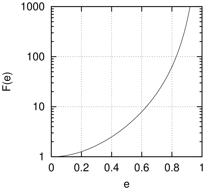
FIG. 1.: Eccentricity factor $F(e)$ (cf. eqn. 57) versus $e$.

REFERENCES

- [1] C. Talmadge, J.-P. Berthias, R. W. Hellings, and E. M. Standish, Phys. Rev. Lett. 61, 1159 (1988).
- [2] A. S. Goldhaber and M. M. Nieto, Phys. Rev. D 9, 1119 (1974).
- [3] M. G. Hare, Can. J. Phys. 51, 431 (1973).
- [4] C. M. Will, Phys. Rev. D 57, 2061 (1998).
- [5] S. L. Larson and W. A. Hiscock, Phys. Rev. D 61, 104008 (2000).
- [6] J. H. Taylor, Rev. Mod. Phys. 66, 711 (1994); Class. Quantum Grav. 10, 167 (1993).
- [7] A. Wolszczan, Nature 350, 688 (1991).
- [8] I. H. Stairs, D. J. Nice, S. E. Thorsett, and J. H. Taylor, astro-ph/9903289.
- [9] M. Visser, Gen. Rel. Grav. 30, 1717 (1998).
- [10] D. G. Boulware and S. Deser, Phys. Rev. D 6, 3368 (1972).
- [11] H. van Dam and M. Veltman, Nucl. Phys. B22, 397 (1970).
- [12] V. I. Zakharov, JETP Lett. 12, 312 (1970).
- [13] R. M. Wald, General Relativity (University of Chicago Press, Chicago, 1984).
- [14] C. W. Misner, K. S. Thorne, and J. A. Wheeler, Gravitation (Freeman, San Francisco, 1973).
- [15] D. E. Krause, H. T. Kloor, and E. Fischbach, Phys. Rev. D 49, 6892 (1994).
- [16] P. C. Peters and J. Mathews, Phys. Rev. B 131, 435 (1963).
- [17] G. J. Feldman and R. D. Cousins, Phys. Rev. D 57, 3873 (1998).
- [18] H. Lück et al., in Gravitational Waves, No. 523 in AIP Conference Proceedings, edited by S. Meshkov (American Institute of Physics, Melville, New York, 2000), pp. 119–127, proceedings of the Third Edoardo Amaldi Conference.
- [19] M. Coles, in Gravitational Waves, No. 523 in AIP Conference Proceedings, edited by S. Meshkov (American Institute of Physics, Melville, New York, 2000), proceedings of the Third Edoardo Amaldi Conference.
- [20] F. Marion and The VIRGO Collaboration, in Gravitational Waves, No. 523 in AIP Conference Proceedings, edited by S. Meshkov (American Institute of Physics, Melville, New York, 2000), pp. 110–118, proceedings of the Third Edoardo Amaldi Conference.
- [21] W. O. Hamilton et al., in Omnidirectional Gravitational Radiation Observatory, edited by W. F. Velloso, Jr., O. D. Aguiar, and N. S. Magalhaes (World Scientific, Singapore, 1997), pp. 19–26.
- [22] M. Cerdonio et al., Class. Quantum Grav. 14, 1491 (1997).
- [23] P. Astone et al., in Omnidirectional Gravitational Radiation Observatory, edited by W. F. Velloso, Jr., O. D. Aguiar, and N. S. Magalhaes (World Scientific, Singapore, 1997), pp. 39–50.
- [24] D. Blair, in Gravitational Waves, No. 523 in AIP Conference Proceedings, edited by S. Meshkov (American Institute of Physics, Melville, New York, 2000), proceedings of the Third Edoardo Amaldi Conference.
- [25] LIGO II Conceptual Project Book, Technical Report No. M990288-A1, The LIGO Project, California Institute of Technology (unpublished), available at http://www.ligo.caltech.edu/docs/M/M990288-A1.pdf.
- [26] A. de Waard and G. Frossati, in Gravitational Waves, No. 523 in AIP Conference Proceedings, edited by S. Meshkov (American Institute of Physics, Melville, New York, 2000), proceedings of the Third Edoardo Amaldi Conference.
- [27] M. Cerdonio et al., Phys. Rev. Lett. 87, 031101 (2001).
- [28] Proceedings of the First International LISA Symposium (IOP, Oxford, 1997), No. 6.
- [29] Laser Interferometer Space Antenna: Proceedings of the Second International LISA Symposium, No. 456 in AIP Conference Proceedings (American Institute of Physics, Woodbury, NY, 1998).
- [30] V. Kalogera, R. Narayan, D. N. Spergel and J. H. Taylor, Astrophys. J. 556, 340 (2001).