Stability criterion for self-similar solutions with perfect fluids in general relativity

Abstract

A stability criterion is derived for self-similar solutions with perfect fluids which obey the equation of state $P=k\rho$ in general relativity. A wide class of self-similar solutions turn out to be unstable against the so-called kink mode. The criterion is directly related to the classification of sonic points. The criterion gives a sufficient condition for instability of the solution. For a transonic point in collapse, all primary-direction nodal-point solutions are unstable, while all secondary-direction nodal-point solutions and saddle-point ones are stable against the kink mode. The situation is reversed in expansion. Applications are the following: the expanding flat Friedmann solution for $1/3\leq k<1$ and the collapsing one for $0<k\leq 1/3$ are unstable; the static self-similar solution is unstable; nonanalytic self-similar collapse solutions are unstable; the Larson-Penston (attractor) solution is stable for this mode for $0<k\lesssim 0.036$, while it is unstable for $0.036\lesssim k$; the Evans-Coleman (critical) solution is stable for this mode for $0<k\lesssim 0.89$, while it is unstable for $0.89\lesssim k$. The last application suggests that the Evans-Coleman solution for $0.89\lesssim k$ is not critical because it has at least two unstable modes.

I introduction

The invariance under scale transformation is one of the important features of gravitational physics as long-range force in general relativity as well as in Newtonian gravity. The scale invariance of field equations implies the existence of solutions which are invariant under the scale transformation. Such scale-free solutions are called self-similar solutions. Among them, the most widely researched system in general relativity is a spherically symmetric self-similar spacetime with a perfect fluid, which is pioneered by Cahill and Taub [1]. The existence of such solutions requires the equation of state to be the form $P=k\rho$ if it is barotropic. A wide class of matter fields can be modelled by this equation of state. In general relativity, spherically symmetric self-similar solutions are classified with the theory of dynamical systems [2] and with their asymptotic forms [3]. For a recent review, see [4].

Although self-similar solutions form a zero-measure set of solutions to the field equations, several authors conjectured that self-similar solutions play important roles in gravitational collapse and/or in cosmological situations (see, e.g., [5]). In this context, the so-called Larson-Penston self-similar solution has been shown to describe generic gravitational collapse of isothermal gas in Newtonian gravity [6, 7, 8]. This solution was discovered by Penston and independently by Larson [9], and after that generalized to general relativity by Ori and Piran [10, 11]. Actually, Newtonian self-similar solutions are obtained by taking the limit $k\to 0$ of those in general relativity [11]. Recently, it has been shown by numerical simulations and a normal mode analysis that the general relativistic counterpart of the Larson-Penston solution is an attractor solution in general relativistic gravitational collapse [12]. This convergence phenomena, i.e., the generic convergence to a self-similar solution, can be regarded as the recovery of scale-invariance symmetry in gravitational physics because the scale-invariance symmetry which the system of the field equations originally has is regained in gravitational collapse even if the symmetry is lost in the initial situation. In the Larson-Penston solution, a naked singularity develops from regular initial data for $0<k\lesssim 0.0105$ [10, 11]. See also [12, 13] for the relationship between the cosmic censorship conjecture and the nature of the Larson-Penston solution as an attractor.

In addition to the attractive nature of a self-similar solution, the critical behavior in the gravitational collapse discovered by Choptuik [14] shed light on self-similarity (for a recent review, see [15]). He investigated the threshold between the collapse to a black hole and the dispersion to infinity in the self-gravitating system of a massless scalar field. He found critical behavior, such as the mass-scaling law for the formed black hole mass, which is analogous to that in statistical physics. He also found that there is a discrete self-similar solution that sits at the threshold of the black hole formation, which is called a critical solution. After that, Evans and Coleman [16] observed similar phenomena in the collapse of a radiation fluid ($k=1/3$) and found that the critical solution coincides with one of the continuous self-similar solutions with analyticity, which we call Evans-Coleman solution . Recently, their work was extended to $0<k\leq 1$ [17]. A renormalization group approach by Koike et al. [18] gave a simple physical explanation to the critical phenomena and showed that the critical solution is characterized by a single unstable mode for a radiation fluid. After that their work was extended to $0<k\leq 0.889$ [19]. The detailed characteristics of the Evans-Coleman solution for $0<k\leq 1$ was investigated [17, 20]. Moreover, ‘Hunter (a)’ self-similar solution, which was originally discovered by Hunter [21], was identified with the Newtonian counterpart of the Evans-Coleman solution [7, 12].

For Newtonian self-similar solutions, Ori and Piran [22] pointed out the existence of kink instability in a wide class of self-similar solutions. The kink mode results from the existence of sonic points. The nature of sonic points was examined in Newtonian gravity [23] and in general relativity [11, 24, 25, 26]. The kink mode corresponds to the injection of a weak discontinuity at sonic points at some initial moment. The instability is characterized by the divergence of the discontinuity in a finite time interval. The blow-up of this mode implies shock wave formation. Unfortunately, the analysis was restricted to Newtonian gravity and applies at most to the case $0<k\ll 1$ [11]. In this paper, the analysis is generalized to fully general relativistic case. The stability criterion obtained here applies even to the case for any value of $k$ ($0<k<1$). Then, we can deal with highly relativistic situations, such as the collapse of a radiation fluid, the evolution of early universe, and so on. The obtained criterion gives a sufficient condition for instability and a necessary condition for stability, because the analysis is specified on the kink mode. Of course, the present analysis reproduces the previously obtained results in Newtonian gravity.

The organization of this paper is the following. In Section II, basic equations are presented. In Section III, the classification of sonic points are reviewed, which is closely related to the kink instability. In Section IV, the stability for the kink mode is analyzed in full order, and a stability criterion for this mode is derived. In Section V, applications to known self-similar solutions, such as the flat Friedmann solution, static self-similar solution, Larson-Penston solution and Evans-Coleman solution, are presented. In Section VI, we comment on recent numerical works by Neilsen and Choptuik [17] and discuss two interesting limiting cases. Section VII is devoted to summary. We adopt units such that $G=c=1$.

II Basic Equations

A Einstein’s Equations

In this section, we basically follow the formulation on a spherically symmetric self-similar system given by Bicknell and Henriksen [24]. It is noted that there are several different formulations (see, e.g., [2, 3, 11]).

The line element in a spherically symmetric spacetime is given by

$$ds^{2}=-e^{\sigma(t,r)}dt^{2}+e^{\omega(t,r)}dr^{2}+R^{2}(t,r)(d\theta^{2}+\sin^{2}\theta d\phi^{2}).$$ (1)

We consider a perfect fluid as a matter field

$$T^{\mu\nu}=(\rho+P)u^{\mu}u^{\nu}+Pg^{\mu\nu}.$$ (2)

Here we adopt the comoving coordinates. Then Einstein’s equations and the equations of motion for the matter field are reduced to the following partially differential equations (PDE’s):

$$\frac{\partial\sigma}{\partial r}=-\frac{2}{\rho+P}\frac{\partial P}{\partial r},$$ (3)

$$\frac{\partial\omega}{\partial t}=-\frac{2}{\rho+P}\frac{\partial\rho}{\partial t}-\frac{4}{R}\frac{\partial R}{\partial t},$$ (4)

$$\frac{\partial m}{\partial r}=4\pi R^{2}\rho\frac{\partial R}{\partial r},$$ (5)

$$\frac{\partial m}{\partial t}=-4\pi R^{2}P\frac{\partial R}{\partial t},$$ (6)

$$e^{-\sigma}\left(\frac{\partial^{2}R}{\partial t^{2}}-\frac{1}{2}\frac{\partial\sigma}{\partial t}\frac{\partial R}{\partial t}\right)-\frac{1}{2}e^{-\omega}\frac{\partial\sigma}{\partial r}\frac{\partial R}{\partial r}=-\frac{m}{R^{2}}-4\pi PR,$$ (7)

and

$$m=\frac{R}{2}\left[1+e^{-\sigma}\left(\frac{\partial R}{\partial t}\right)^{2}-e^{-\omega}\left(\frac{\partial R}{\partial r}\right)^{2}\right],$$ (8)

where $m(t,r)$ is called Misner-Sharp mass and five of the above six equations are independent.

We assume the following equation of state:

$$P=k\rho,$$ (9)

where we assume $0<k<1$. We define dimensionless functions such as

$$\eta \equiv 8\pi r^{2}\rho,$$ (10)

$$S \equiv \frac{R}{r},$$ (11)

$$M \equiv \frac{2m}{r}.$$ (12)

We also define the following self-similar coordinate:

$$\xi\equiv\frac{t}{r}.$$ (13)

It is often more convenient to use the following coordinates:

$$\tau \equiv -\ln|t|,$$ (14)

$$z \equiv -\ln|\xi|.$$ (15)

It is noted that $\xi$ is a two-valued function of $z$, such as $z=-\infty$ corresponds to $\xi=\pm\infty$ and $z=+\infty$ corresponds to $\xi=\pm 0$.

It is found that equations (3) and (4) are integrated as

$$e^{\sigma} = a_{\sigma}(t)(\eta e^{-2z})^{-\frac{2k}{1+k}},$$ (16)

$$e^{\omega} = a_{\omega}(r)\eta^{-\frac{2}{1+k}}S^{-4},$$ (17)

where $a_{\sigma}(t)$ and $a_{\omega}(r)$ are arbitrary functions. These functions correspond to the freedom of re-scaling the time and radial coordinates as $\tilde{t}=\tilde{t}(t)$ and $\tilde{r}=\tilde{r}(t)$. Using this freedom, we let $a_{\sigma}$ and $a_{\omega}$ be constant.

For later convenience, we define a quantity $y$ as

$$y\equiv\frac{M}{\eta S^{3}},$$ (18)

which has a clear physical meaning that it is one third of the ratio of the ‘averaged density’ of the region interior to $(t,r)$ to the local density at $(t,r)$. We also define two velocity functions $V$ and $V_{R}$. The $V$ is the velocity of the $\xi=\mbox{const}$ curve relative to the fluid element, which is written as

$$V=\mbox{sign}(\xi)e^{z+\frac{\omega-\sigma}{2}},$$ (19)

while $V_{R}$ is the velocity of the $R=\mbox{const}$ curve relative to the fluid element, which is written as

$$V_{R}\equiv-e^{\frac{\omega-\sigma}{2}}\frac{\left(\frac{\partial R}{\partial t}\right)}{\left(\frac{\partial R}{\partial r}\right)}=V\frac{\dot{S}+S^{\prime}}{S+S^{\prime}},$$ (20)

where

^⋅ $$\equiv \frac{\partial}{\partial\tau},$$ (21)

^′ $$\equiv \frac{\partial}{\partial z}.$$ (22)

$V$ is written as

$$V^{2}=\frac{a_{\omega}}{a_{\sigma}}(\eta e^{-z})^{-2\frac{1-k}{1+k}}S^{-4}.$$ (23)

Using these dimensionless variables, equations (5)-(8) are reduced to the following form:

$$M+M^{\prime}=\eta S^{2}(S+S^{\prime}),$$ (26)

$$\dot{M}+M^{\prime}=-k\eta S^{2}(\dot{S}+S^{\prime}),$$

$$\ddot{S}+2\dot{S}^{\prime}+S^{\prime\prime}+\left[\frac{k}{1+k}\left(\frac{\dot{\eta}}{\eta}+\frac{\eta^{\prime}}{\eta}-2\right)+1\right](\dot{S}+S^{\prime})$$

$$= -\frac{k}{1+k}e^{\sigma-\omega-2z}\left(\frac{\eta^{\prime}}{\eta}-2\right)(S+S^{\prime})-\frac{1}{2}e^{\sigma-2z}\frac{M+k\eta S^{3}}{S^{2}},$$ (27)

and

$$\frac{M}{S}=1+e^{-\sigma+2z}(\dot{S}+S^{\prime})^{2}-e^{-\omega}(S+S^{\prime})^{2},\\$$ (28)

where three of the above four equations are independent.

B Self-similarity

For self-similar solutions, we assume that all dimensionless quantities depend only on $z$, i.e., $M=M(z)$, $S=S(z)$, $\eta=\eta(z)$, $\sigma=\sigma(z)$, and $\omega=\omega(z)$. Then, from equations (26)-(28), we obtain the following ordinary differential equations (ODE’s):

$$M^{\prime} = \frac{k}{1+k}\frac{1-y}{y}M,$$ (29)

$$S^{\prime} = -\frac{1-y}{1+k}S,$$ (30)

$$\eta^{\prime} = \left[2(1-y)-2\frac{ky-\frac{1}{4}(1+k)^{2}e^{\omega}\eta}{V^{2}-k}\right]\eta,$$ (31)

and constraint equation

$$V^{2}(1-y)^{2}-(k+y)^{2}+(1+k)^{2}e^{\omega}S^{-2}(1-y\eta S^{2})=0.$$ (32)

From equations (20) and (30), we find

$$V_{R}=-V\frac{1-y}{k+y}.$$ (33)

III Sonic points

The classification of sonic points in general relativity was studied by Bicknell and Henriksen ([24]; see also [11, 25, 26]). Here we briefly review their work, which turn out to be closely related to the stability criterion of the kink mode.

A Regularity

The sonic point is defined by

$$V^{2}=k,$$ (34)

that is, $V$ is equal to the sound speed. At the sonic point, the system of the ODE’s (29)-(31) is singular. Since $V$ is the relative velocity of the $\xi=\mbox{const}$ curve to the fluid element, informations with the sound speed propagate only outward or inward for $V^{2}>k$, while in both directions for $V^{2}<k$, in terms of $\xi$. In this sense, the former is supersonic, while the latter is subsonic, in terms of $\xi$. Hence, informations can cross the sonic point only in a single direction. This is a physical reason why the system of the ODE’s becomes singular at the sonic point.

First, we consider the regularity condition at the sonic point. The regularity requires

$$ky-\frac{1}{4}(1+k)^{2}e^{\omega}\eta=0.$$ (35)

From equations (32), (34) and (35), we find the following explicit relations at the sonic point

$$e^{-z_{s}} = \left[\frac{(k+y_{s})^{2}+k(3y_{s}-1)(1+y_{s})}{a_{\sigma}^{\frac{1+3k}{2(1-k)}}a_{\omega}^{-\frac{1}{2}}(1+k)^{\frac{4k}{1-k}}k^{\frac{3}{2}}(4y_{s})^{\frac{1-3k}{1-k}}}\right]^{\frac{1+k}{1+3k}},$$ (36)

$$M_{s} = y_{s}\eta_{s}S^{3}_{s},$$ (37)

$$S_{s} = \left[\frac{a_{\sigma}a_{\omega}(1+k)^{4}}{k(4y_{s})^{2}}\right]^{\frac{1}{4}}e^{-\frac{1-k}{2(1+k)}z_{s}},$$ (38)

$$\eta_{s} = \left[\frac{4y_{s}}{a_{\sigma}(1+k)^{2}}\right]^{\frac{1+k}{1-k}}e^{2z_{s}}.$$ (39)

Therefore, sonic points are parametrized by one parameter $y_{s}$. Equation (36) requires the following condition:

$$y_{s}>y_{1}\equiv\frac{-2k+\sqrt{k(1+6k-3k^{2})}}{1+3k}.$$ (40)

B Classification of sonic points

We introduce new independent variable $u$ which is defined as

$$-\frac{dz}{du}=V^{2}-k.$$ (41)

Using $u$ in place of $z$, a sonic point turns out to be a stationary point (or a singular point) of the resultant system of the ODE’s as

$$\frac{dM}{du} = -\frac{k}{1+k}\frac{1-y}{y}(V^{2}-k)M,$$ (42)

$$\frac{dS}{du} = \frac{1-y}{1+k}(V^{2}-k)S,$$ (43)

$$\frac{d\eta}{du} = -\left[2(1-y)(V^{2}-k)-2\left(ky-\frac{1}{4}(1+k)^{2}e^{\omega}\eta\right)\right]\eta,$$ (44)

A stationary point is classified by the behavior of solutions around the point. We put

$$M = \eta_{s}S_{s}^{3}(y+x_{1}),$$ (45)

$$S = S_{s}(1+x_{2}),$$ (46)

$$\eta = \eta_{s}(1+x_{3}),$$ (47)

$$\xi = \xi_{s}(1+x_{4}),$$ (48)

where $x_{1}$ to $x_{4}$ are regarded as components of the vector ${\bf x}$. Then, we find the following linearized ODE’s in the matrix form:

$$\frac{d}{du}{\bf x}={\bf A}{\bf x},$$ (49)

where the matrix ${\bf A}$ is given by

$${\bf A}=\frac{2k}{1+k}\left(\begin{array}[]{cccc}0&2k(1-y)&k(1-k)(1-y)/(1+k)&k(1-k)(1-y)/(1+k)\\ 0&-2(1-y)&-(1-k)(1-y)/(1+k)&-(1-k)(1-y)/(1+k)\\ 1+k&(4-3y)(1+k)&2(1-k-y)&2(1-k)(1-y)\\ 0&-2(1+k)&-(1-k)&-(1-k)\end{array}\right).$$ (50)

This matrix has two zero eigenvalues and two generically nonzero eigenvalues $\lambda_{\pm}$ ($\lambda_{-}\leq\lambda_{+}$)

$$\lambda_{\pm}=\frac{2k}{1+k}\tilde{\lambda}_{\pm},$$ (51)

where $\tilde{\lambda}_{\pm}$ are given by

$$\tilde{\lambda}_{\pm}=\frac{-(1+k)\pm\sqrt{D}}{2},$$ (52)

with

$$D=1+6k-3k^{2}-4y-24ky+12k^{2}y+4y^{2}+12ky^{2}.$$ (53)

These two eigenvalues $\lambda_{\pm}$ are associated with the corresponding eigenvectors ${\bf e}_{\pm}$, respectively. The sonic point is classified into a saddle for $\lambda_{-}<0<\lambda_{+}$, a nondegenerate node for $\lambda_{-}<\lambda_{+}<0$, a degenerate node for $\lambda_{-}=\lambda_{+}$, and a focus for complex values of $\lambda_{\pm}$. For a saddle, only two solutions pass through it, one along the $+$ive direction ${\bf e}_{+}$ and the other along the $-$ive direction ${\bf e}_{-}$. For a nondegenerate node, there are one-parameter family of solutions which cross the sonic point along the $+$ive direction, while only one solution crosses along the $-$ive direction. The directions $+$ and $-$ for a node are called the primary and secondary directions, respectively. For a degenerate node, two directions $+$ and $-$ coincide with each other. The sonic point which is a focus is unphysical. The sonic point is a nondegenerate node or saddle for $D>0$, a degenerate node for $D=0$, and a focal point for $D<0$. The condition $D\geq 0$ requires

$$y_{s}\leq y_{2}~{}\mbox{or}~{}y_{3}\leq y_{s},$$ (54)

where $y_{2,3}$ ($y_{2}<y_{3}$) are given by

$$y_{2,3}\equiv\frac{1+6k-3k^{2}\mp\sqrt{3k(1-k)(1+6k-3k^{2})}}{2(1+3k)},$$ (55)

and $D=0$ holds only for $y_{s}=y_{2}$ or $y_{s}=y_{3}$. Together with equation (40), since $y_{1}<y_{2}$ can be verified, it is found that

$$y_{1}<y_{s}\leq y_{2}~{}\mbox{or}~{}y_{3}\leq y_{s},$$ (56)

for the sonic point to be physical. Whether the sonic point is a node or saddle is determined by the sign of $[(1+k)^{2}-D]$. It changes its sign at $y_{s}=y_{4}$ or $y_{s}=y_{5}$ ($y_{4}>y_{5}$), where

$$y_{4,5}=\frac{1+6k-3k^{2}\pm\sqrt{(1+4k-k^{2})^{2}+8k^{2}(1-k)^{2}}}{2(1+3k)}.$$ (57)

Since $y_{5}<y_{1}$ can be verified, it is found that the sonic point is unphysical for $y_{s}<y_{1}$ or $y_{2}<y_{s}<y_{3}$, a degenerate node for $y_{s}=y_{2}$ or $y_{s}=y_{3}$, a nondegenerate node for $y_{1}<y_{s}<y_{2}$ or $y_{3}<y_{s}<y_{4}$, and a saddle for $y_{4}<y_{s}$. The classification of sonic points in terms of the parameter $y_{s}$ is plotted in figure 1.

It is seen that, along the allowed directions $\pm$,

$$\frac{\eta^{\prime}}{\eta}=\frac{3-k-2y+\tilde{\lambda}_{\pm}}{1-k}$$ (58)

at the sonic point. Using this and the relation

$$\frac{V^{\prime}}{V}=-\frac{1-k}{1+k}\frac{\eta^{\prime}}{\eta}+\frac{3-k-2y}{1+k},$$ (59)

which follows from equations (23) and (30), it is found that

$$(V^{2})^{\prime}=-\lambda_{\pm},$$ (60)

or

$$\frac{V^{\prime}}{V}=\frac{1}{2}\mp\frac{\sqrt{D}}{2(1+k)},$$ (61)

where and hereafter the upper and lower signs denote the $+$ive and $-$ive directions, respectively. Therefore, if a solution crosses a saddle sonic point from subsonic interior to supersonic exterior, then it goes along the $-$ive direction. A sonic point with subsonic interior and supersonic exterior is called a ‘transonic’ point. If we consider a solution with regular center and sonic points, the solution must have at least one transonic point. In principle, a solution may have other kinds of sonic points, such as the one with supersonic interior and subsonic exterior which we call an anti-transonic point. It is found that the sonic point with supersonic interior and subsonic exterior must be a saddle and the solution passes it along the $+$ive direction. Furthermore, it is found that $V^{\prime}/V<1/2$ or $(V^{2})^{\prime}<k$ for the $+$ive direction, $V^{\prime}/V>1/2$ or $(V^{2})^{\prime}>k$ for the $-$ive direction, and $V^{\prime}/V=1/2$ or $(V^{2})^{\prime}=k$ for a degenerate node.

C Analyticity

Furthermore we can require the analyticity condition (Taylor-series expandability) at the sonic point, i.e.,

$$M = M_{s}+M_{s,1}(z-z_{s})+M_{s,2}(z-z_{s})^{2}+\cdots,$$ (62)

$$S = S_{s}+S_{s,1}(z-z_{s})+S_{s,2}(z-z_{s})^{2}+\cdots,$$ (63)

$$\eta = \eta_{s}+\eta_{s,1}(z-z_{s})+\eta_{s,2}(z-z_{s})^{2}+\cdots,$$ (64)

around the sonic point. From equations (29)-(32), we find

$$M_{s,1} = \frac{k}{1+k}\frac{y_{s}}{1-y_{s}}M_{s},$$ (65)

$$S_{s,1} = -\frac{1-y_{s}}{1+k}S_{s},$$ (66)

$$\eta_{s,1} = -\frac{(3k+4y_{s}-5)\mp\sqrt{D}}{2(1-k)}\eta_{s},$$ (67)

if $D$ is not negative. It is found that the upper and lower signs correspond to the $+$ive and $-$ive directions, respectively. In other words, there are two analytic solutions at a sonic point, one of which crosses the sonic point along the $+$ive direction and the other along the $-$ive direction. Since all coefficients of Taylor series are determined only by $M_{s}$, $S_{s}$ and $\eta_{s}$, the analytic solution with each direction is unique for given $y_{s}$. Hence, for a saddle, two solutions pass it and both of them are analytic. On the other hand, for a nondegenerate node, one analytic solution and one-parameter family of nonanalytic solutions pass it along the primary direction, while one solution passes it along the secondary direction and this solution is analytic. In particular, all nonanalytic solutions must cross nodes and go along the primary direction.

IV Kink Instability

A Equations for kink mode

We consider perturbations which satisfy the following conditions in the background of a self-similar solution: (1) The initial perturbations vanish inside the sonic point for $t<0$. (For $t>0$, the initial perturbations vanish outside the sonic point.) (2) $M$, $S$ and $\eta$ are continuous everywhere, in particular at the sonic point. (3) $\eta^{\prime}$ is discontinuous at the sonic point, although it has definite one-sided values as $z\to z_{s}-0$ and $z\to z_{s}+0$.

We denote the full order perturbations as

$$\delta S(\tau,z) = S(\tau,z)-S_{b}(z),$$ (68)

$$\delta M(\tau,z) = M(\tau,z)-M_{b}(z),$$ (69)

$$\delta\eta(\tau,z) = \eta(\tau,z)-\eta_{b}(z),$$ (70)

where $M_{b}$, $S_{b}$ and $\eta_{b}$ denote the background self-similar solution. Hereafter we often omit the subscript ‘$b$’ unless the omission may cause confusion. By conditions (2) and (3), and from equations (26) and (26), it is found that $\delta M^{\prime}$ and $\delta S^{\prime}$ are also continuous. Hence, the perturbations satisfy $\delta M=0,\delta S=0,\delta\eta=0,\delta M^{\prime}=0,\delta S^{\prime}=0,\delta\eta^{\prime}\neq 0$ at the sonic point at initial moment $\tau=\tau_{0}$, where the prime denotes the derivative with respect to $z$ on the perturbed side. The evolution of the initially unperturbed region is completely described by the background self-similar solution because no information from the perturbed side can penetrate the unperturbed side by condition (1). Then, by conditions (2) and (3), we find $\delta M=0,\delta S=0,\delta\eta=0,\delta\dot{M}=0,\delta\dot{S}=0,\delta\dot{\eta}=0,\delta\dot{M}^{\prime}=0,\delta\dot{S}^{\prime}=0,\delta\dot{\eta}^{\prime}\neq 0,$ at the sonic point for $\tau\geq\tau_{0}$ for the case of $t<0$ (for $\tau\leq\tau_{0}$ for the case of $t>0$). This mode has a physical meaning that it injects discontinuity into the density gradient. In fact, the density gradient with respect to the physical length $dl\equiv e^{\omega/2}dr$ on the $t=\mbox{const}$ spacelike hypersurface is directly related to $\eta^{\prime}$ as

$$\left.\frac{\partial\rho}{\partial l}\right|_{t}=\left.e^{-\omega/2}\frac{\partial}{\partial r}\right|_{t}\frac{\eta}{8\pi r^{2}}=\frac{1}{8\pi r^{3}}e^{-\omega/2}(\eta^{\prime}-2\eta).$$ (71)

Differentiating equations (26) and (26) with respect to $z$ and estimating both sides at the point of discontinuity, we obtain the following equations for the full order perturbations:

$$\frac{\delta M^{\prime\prime}}{M} = \frac{k}{1+k}\frac{1}{y}\frac{\delta\eta^{\prime}}{\eta},$$ (72)

$$\frac{\delta S^{\prime\prime}}{S} = -\frac{y}{1+k}\frac{\delta\eta^{\prime}}{\eta}.$$ (73)

We also differentiate equation (27) with respect to $z$. The result is

$$\frac{\ddot{S}^{\prime}}{S}+2\frac{\dot{S}^{\prime\prime}}{S}+\frac{S^{\prime\prime\prime}}{S}+\frac{k}{1+k}\left(\frac{\dot{\eta}^{\prime}}{\eta}-\frac{\dot{\eta}}{\eta}\frac{\eta^{\prime}}{\eta}+\frac{\eta^{\prime\prime}}{\eta}-\frac{\eta^{\prime 2}}{\eta^{2}}\right)\left(\frac{\dot{S}}{S}+\frac{S^{\prime}}{S}\right)$$ (75)

$$+\left[\frac{k}{1+k}\left(\frac{\dot{\eta}}{\eta}+\frac{\eta^{\prime}}{\eta}-2\right)+1\right]\left(\frac{\dot{S}^{\prime}}{S}+\frac{S^{\prime\prime}}{S}\right)$$

$$= -\frac{k}{1+k}e^{\sigma-\omega-2z}\left[\left[-\frac{2k}{1+k}\left(\frac{\eta^{\prime}}{\eta}-2\right)+\frac{2}{1+k}\frac{\eta^{\prime}}{\eta}+4\frac{S^{\prime}}{S}-2\right]\left(\frac{\eta^{\prime}}{\eta}-2\right)\left(1+\frac{S^{\prime}}{S}\right)\right.$$ (79)

$$\left.+\left(\frac{\eta^{\prime\prime}}{\eta}-\frac{\eta^{\prime 2}}{\eta^{2}}\right)\left(1+\frac{S^{\prime}}{S}\right)+\left(\frac{\eta^{\prime}}{\eta}-2\right)\left(\frac{S^{\prime}}{S}+\frac{S^{\prime\prime}}{S}\right)\right]$$

$$-\frac{1}{2}e^{\sigma-2z}\left[\left[-\frac{2k}{1+k}\left(\frac{\eta^{\prime}}{\eta}-2\right)-2\right]\left(\frac{M}{S^{3}}+k\eta\right)\right.$$

$$\left.+\left(\frac{M^{\prime}}{S^{3}}+k\eta^{\prime}+3k\eta\frac{S^{\prime}}{S}\right)-2\frac{S^{\prime}}{S}\left(\frac{M}{S^{3}}+k\eta\right)\right].$$

We find from equations (27) and (79) for the full order perturbations at the point of discontinuity

$$\frac{\delta S^{\prime\prime}}{S}+\frac{k}{1+k}\frac{S^{\prime}}{S}\frac{\delta\eta^{\prime}}{\eta}=-\frac{kV^{-2}}{1+k}\left(1+\frac{S^{\prime}}{S}\right)\frac{\delta\eta^{\prime}}{\eta},$$ (82)

$$2\frac{\delta\dot{S}^{\prime\prime}}{S}+\frac{\delta S^{\prime\prime\prime}}{S}+\frac{k}{1+k}\left(\frac{\delta\dot{\eta}^{\prime}}{\eta}+\frac{\delta\eta^{\prime\prime}}{\eta}-\frac{\delta\eta^{\prime 2}}{\eta^{2}}-2\frac{\eta^{\prime}}{\eta}\frac{\delta\eta^{\prime}}{\eta}\right)\frac{S^{\prime}}{S}$$

$$+\left[\frac{k}{1+k}\left(\frac{\eta^{\prime}}{\eta}-2\right)+1\right]\frac{\delta S^{\prime\prime}}{S}+\frac{k}{1+k}\frac{\delta\eta^{\prime}}{\eta}\frac{S^{\prime\prime}}{S}+\frac{k}{1+k}\frac{\delta\eta^{\prime}}{\eta}\frac{\delta S^{\prime\prime}}{S}$$

$$= -\frac{kV^{-2}}{1+k}\left[2\frac{1-k}{1+k}\frac{\delta\eta^{\prime}}{\eta}\left(\frac{\eta^{\prime}}{\eta}-2\right)\left(1+\frac{S^{\prime}}{S}\right)+2\frac{1-k}{1+k}\left(1+\frac{S^{\prime}}{S}\right)\frac{\delta\eta^{\prime 2}}{\eta^{2}}\right.$$ (87)

$$+\left[-\frac{2k}{1+k}\left(\frac{\eta^{\prime}}{\eta}-2\right)+\frac{2}{1+k}\frac{\eta^{\prime}}{\eta}+4\frac{S^{\prime}}{S}-2\right]\frac{\delta\eta^{\prime}}{\eta}\left(1+\frac{S^{\prime}}{S}\right)$$

$$+\left(\frac{\delta\eta^{\prime\prime}}{\eta}-2\frac{\eta^{\prime}}{\eta}\frac{\delta\eta^{\prime}}{\eta}-\frac{\delta\eta^{\prime 2}}{\eta^{2}}\right)\left(1+\frac{S^{\prime}}{S}\right)$$

$$\left.+\frac{\delta\eta^{\prime}}{\eta}\left(\frac{S^{\prime}}{S}+\frac{S^{\prime\prime}}{S}\right)+\left(\frac{\eta^{\prime}}{\eta}-2\right)\frac{\delta S^{\prime\prime}}{S}+\frac{\delta\eta^{\prime}}{\eta}\frac{\delta S^{\prime\prime}}{S}\right]$$

$$-\frac{1}{2}e^{\omega}\eta V^{-2}\left[-\frac{2k}{1+k}\frac{\delta\eta^{\prime}}{\eta}(y+k)+k\frac{\delta\eta^{\prime}}{\eta}\right].$$

At the sonic point, equation (82) is reduced to

$$\frac{\delta S^{\prime\prime}}{S}+\frac{y}{1+k}\frac{\delta\eta^{\prime}}{\eta}=0,$$ (88)

which is equivalent to equation (73). Therefore, it is found that the injection of this type of discontinuity into the density gradient field is possible only at the sonic point. Next, we evaluate both sides of equation (87) at the sonic point using equations (34) and (35). One can observe that there appear $\delta S^{\prime\prime\prime}$ and $\delta\eta^{\prime\prime}$ in this equation. It is easily found that such terms appear in the equation only through the following combination:

$$\frac{\delta S^{\prime\prime\prime}}{S}+\frac{y}{1+k}\frac{\delta\eta^{\prime\prime}}{\eta}.$$ (89)

In order to write these terms using the lower order derivatives, we eliminate $M^{\prime}$ from equations (26) and (26) as

$$M-\dot{M}=\eta S^{3}+(1+k)\eta S^{2}S^{\prime}+k\eta S^{2}\dot{S}.$$ (90)

Differentiating the above equation twice with respect to $z$, we have

$$M^{\prime\prime}-\dot{M}^{\prime\prime}$$ (91)

$$= \eta^{\prime\prime}S^{3}+6\eta^{\prime}S^{2}S^{\prime}+6\eta SS^{\prime 2}+3\eta S^{2}S^{\prime\prime}$$ (94)

$$+(1+k)(\eta^{\prime\prime}S^{2}S^{\prime}+4\eta^{\prime}SS^{\prime 2}+2\eta^{\prime}S^{2}S^{\prime\prime}+2\eta S^{\prime 3}+6\eta SS^{\prime}S^{\prime\prime}+\eta S^{2}S^{\prime\prime\prime})$$

$$+k(\eta^{\prime\prime}S^{2}\dot{S}+4\eta^{\prime}SS^{\prime}\dot{S}+2\eta^{\prime}S^{2}\dot{S}^{\prime}+2\eta S^{\prime 2}\dot{S}+2\eta SS^{\prime\prime}\dot{S}+4\eta SS^{\prime}\dot{S}^{\prime}+\eta S^{2}\dot{S}^{\prime\prime}).$$

Estimating the full order perturbations of both sides at the sonic point, we find

$$\frac{\delta S^{\prime\prime\prime}}{S}+\frac{y}{1+k}\frac{\delta\eta^{\prime\prime}}{\eta}$$ (95)

$$= \frac{y}{1+k}\left[\frac{\delta M^{\prime\prime}}{M}-\frac{\delta\dot{M}^{\prime\prime}}{M}\right]-\frac{k}{1+k}\frac{\delta\dot{S}^{\prime\prime}}{S}-2\left[\frac{3}{1+k}\frac{S^{\prime}}{S}+2\left(\frac{S^{\prime}}{S}\right)^{2}+\frac{S^{\prime\prime}}{S}\right]\frac{\delta\eta^{\prime}}{\eta}$$ (97)

$$-\left[\frac{3}{1+k}+2\left(\frac{\eta^{\prime}}{\eta}+3\frac{S^{\prime}}{S}\right)\right]\frac{\delta S^{\prime\prime}}{S}-2\frac{\delta\eta^{\prime}}{\eta}\frac{\delta S^{\prime\prime}}{S}.$$

Using the above relation, we evaluate both sides of equation (87) at the sonic point using $\delta M^{\prime\prime}$, $\delta S^{\prime\prime}$ and $\delta\eta^{\prime}$. After a rather lengthy calculation, we obtain the following equation:

$$\frac{\delta\dot{\eta}^{\prime}}{\eta}+\left(-2\frac{1-k}{1+k}\frac{\eta^{\prime}}{\eta}+\frac{5-3k-4y}{1+k}\right)\frac{\delta\eta^{\prime}}{\eta}-\frac{1-k}{1+k}\left(\frac{\delta\eta^{\prime}}{\eta}\right)^{2}=0.$$ (98)

It is noted that the PDE’s become an ODE for the discontinuity in the density gradient at the sonic point. This is due to the nature of the sonic point. It is more convenient to rewrite this in terms of $V^{\prime}$ and $\delta V^{\prime}$ using the relation (59). The discontinuity in $V^{\prime}$ is directly related to the discontinuity in $\delta\eta^{\prime}$ through

$$\frac{\delta V^{\prime}}{V}=-\frac{1-k}{1+k}\frac{\delta\eta^{\prime}}{\eta}.$$ (99)

Finally we obtain the following equation for the full order perturbation as

$$\frac{\delta\dot{V}^{\prime}}{V}-\left[1-2\left(\frac{V^{\prime}}{V}\right)_{b}\right]\frac{\delta V^{\prime}}{V}+\left(\frac{\delta V^{\prime}}{V}\right)^{2}=0.$$ (100)

It is noted that the above equation has complete correspondence to its Newtonian counterpart, equation (15) of [22], when the latter is rewritten in terms of the relative velocity of the constant self-similar coordinate curve to the fluid element.

B Linear order analysis

By linearizing equation (100), we can obtain

$$\frac{\delta\dot{V}^{\prime}}{V}=\left[1-2\left(\frac{V^{\prime}}{V}\right)_{b}\right]\frac{\delta V^{\prime}}{V}.$$ (101)

This equation is integrated as

$$\frac{\delta V^{\prime}}{V}=\mbox{const}\cdot e^{\alpha\tau},$$ (102)

where

$$\alpha\equiv 1-2\left(\frac{V^{\prime}}{V}\right)_{b}.$$ (103)

Therefore, it is found that the discontinuity in $V^{\prime}$ grows for $\alpha>0$, decays for $\alpha<0$ and the mode is neutral for $\alpha=0$ as $\tau$ increases. On the other hand, it is found that the discontinuity in $V^{\prime}$ grows for $\alpha<0$, decays for $\alpha>0$ and the mode is neutral for $\alpha=0$ as $\tau$ decreases. The above discussion will suggest some kind of instability. Nevertheless, the linear order analysis will not be sufficient in this case from the following reason. The discontinuity in the density gradient which is injected as a perturbation may not be included in the background solution. Then, there is no natural measure how much the perturbation grows compared with the background solution. In the linear order analysis, we can show at most a power-law growth of the discontinuity for sufficiently small perturbation. In the next subsection, we will show a divergence of full order perturbation at some finite moment, even if initial perturbation is small. This does indicate instability.

C Full order analysis

In fact, equation (100) is easily integrated. Putting

$$X \equiv \frac{\delta V^{\prime}}{V},$$ (104)

we rewrite equation (100) as

$$\dot{X}-\alpha X+X^{2}=0.$$ (105)

There are two stationary solutions $X=0$ and $X=\alpha$. General solutions are the following:

$$X = \frac{\alpha}{1-\exp(-\alpha\tau+\mbox{const})},\quad\mbox{for}\quad\alpha\neq 0,$$ (106)

$$X = \frac{1}{\tau+\mbox{const}},\quad\mbox{for}\quad\alpha=0.$$ (107)

For an initial value $X=X_{0}\neq 0$ at $\tau=\tau_{0}$, the solution is written as

$$\frac{1}{X} = \frac{1}{\alpha}-e^{-\alpha(\tau-\tau_{0})}\left(\frac{1}{\alpha}-\frac{1}{X_{0}}\right),\quad\mbox{for}\quad\alpha\neq 0,$$ (108)

$$\frac{1}{X} = \frac{1}{X_{0}}+(\tau-\tau_{0}),\quad\mbox{for}\quad\alpha=0.$$ (109)

1 $D>0$ case

First, we consider $\alpha>0$. From equation (108), it is seen that, as $\tau$ increases, $X$ blows up to $-\infty$ at some finite moment $\tau\to\tau_{d}-0>\tau_{0}$ for $X_{0}<0$, where

$$\tau_{d}\equiv\tau_{0}+\frac{1}{\alpha}\ln\left(1-\frac{\alpha}{X_{0}}\right),$$ (110)

while $X$ monotonically approaches $\alpha$ for $X_{0}>0$. Next, we consider $\alpha<0$. From equation (108), it is seen that, as $\tau$ increases, $X$ monotonically approaches $0$ for $X_{0}>\alpha$, while $X$ blows up to $-\infty$ at some finite moment $\tau=\tau_{d}-0>\tau_{0}$ for $X_{0}<\alpha$.

Actually these two analyses under two different backgrounds are only apparently different local pictures of nonlinear dynamics. If we consider the background solution which crosses the sonic point along the $+$ive direction, $\alpha$ is positive and the stationary solution $X=\alpha$ corresponds to another possible direction, since

$$\left(\frac{V^{\prime}}{V}\right)_{-}=\left(\frac{V^{\prime}}{V}\right)_{+}+\left[1-2\left(\frac{V^{\prime}}{V}\right)_{+}\right].$$ (111)

The situation is reversed for the $-$ive direction solution, since

$$\left(\frac{V^{\prime}}{V}\right)_{+}=\left(\frac{V^{\prime}}{V}\right)_{-}+\left[1-2\left(\frac{V^{\prime}}{V}\right)_{-}\right].$$ (112)

The global picture is the following. With the initial value $V^{\prime}/V=(V^{\prime}/V)_{0}$ at $\tau=\tau_{0}$, we obtain the following full order behavior of the perturbation:

$$\frac{V^{\prime}}{V} \to -\infty\quad\mbox{as}\quad\tau\to\tau_{d}-0\quad\mbox{for}\quad\left(\frac{V^{\prime}}{V}\right)_{0}<\left(\frac{V^{\prime}}{V}\right)_{+},$$ (113)

$$\frac{V^{\prime}}{V} = \left(\frac{V^{\prime}}{V}\right)_{+}=\mbox{const}\quad\mbox{for}\quad\left(\frac{V^{\prime}}{V}\right)_{0}=\left(\frac{V^{\prime}}{V}\right)_{+},$$ (114)

$$\frac{V^{\prime}}{V} \to \left(\frac{V^{\prime}}{V}\right)_{-}\quad\mbox{as}\quad\tau\to\infty\quad\mbox{for}\quad\left(\frac{V^{\prime}}{V}\right)_{+}<\left(\frac{V^{\prime}}{V}\right)_{0},$$ (115)

as $\tau$ increases, while

$$\frac{V^{\prime}}{V} \to \left(\frac{V^{\prime}}{V}\right)_{+}\quad\mbox{as}\quad\tau\to-\infty\quad\mbox{for}\quad\left(\frac{V^{\prime}}{V}\right)_{0}<\left(\frac{V^{\prime}}{V}\right)_{-},$$ (116)

$$\frac{V^{\prime}}{V} = \left(\frac{V^{\prime}}{V}\right)_{-}=\mbox{const}\quad\mbox{for}\quad\left(\frac{V^{\prime}}{V}\right)_{0}=\left(\frac{V^{\prime}}{V}\right)_{-},$$ (117)

$$\frac{V^{\prime}}{V} \to \infty\quad\mbox{as}\quad\tau\to\tau_{d}+0\quad\mbox{for}\quad\left(\frac{V^{\prime}}{V}\right)_{-}<\left(\frac{V^{\prime}}{V}\right)_{0},$$ (118)

as $\tau$ decreases. The dynamical behavior of the perturbation is schematically depicted in figure 2.

2 $D=0$ case

We consider $\alpha=0$. From equation (109), it is seen that, as $\tau$ increases, $X$ diverges to $-\infty$ at some finite moment $\tau\to\tau_{d}$, where

$$\tau_{d}\equiv\tau_{0}-\frac{1}{X_{0}},$$ (119)

for $X_{0}<0$, while $X$ approaches $0$ for $X_{0}>0$.

This case corresponds to a degenerate node for which $D=0$ and $(V^{\prime}/V)_{b}=1/2$. Then we find

$$\frac{V^{\prime}}{V} \to -\infty\quad\mbox{as}\quad\tau\to\tau_{d}-0\quad\mbox{for}\quad\left(\frac{V^{\prime}}{V}\right)_{0}<\frac{1}{2},$$ (120)

$$\frac{V^{\prime}}{V} \to \frac{1}{2}\quad\mbox{as}\quad\tau\to\infty\quad\mbox{for}\quad\frac{1}{2}\leq\left(\frac{V^{\prime}}{V}\right)_{0},$$ (121)

as $\tau$ increases, while

$$\frac{V^{\prime}}{V} \to \frac{1}{2}\quad\mbox{as}\quad\tau\to-\infty\quad\mbox{for}\quad\left(\frac{V^{\prime}}{V}\right)_{0}\leq\frac{1}{2},$$ (122)

$$\frac{V^{\prime}}{V} \to \infty\quad\mbox{as}\quad\tau\to\tau_{d}+0\quad\mbox{for}\quad\frac{1}{2}<\left(\frac{V^{\prime}}{V}\right)_{0},$$ (123)

as $\tau$ decreases. The behavior is depicted in figure 3.

D Stability criterion

First, we consider $t<0$. The time evolution is regarded as the increase of $\tau$ from $\tau=\tau_{0}$. Then, we obtain the following criterion: all $+$ive direction solutions and degenerate-nodal-point ones are unstable, while all $-$-direction solutions are stable for this mode. Next, we consider the case $t>0$. In that case, the time evolution is regarded as the decrease of $\tau$ from $\tau=\tau_{0}$. Then, we find the following criterion: all $-$-direction solutions and degenerate-nodal-point ones are unstable, while all $+$-direction solutions are stable for this mode. These are summarized in table I.

The stability criterion which applies to all possible situations is the following: if $V^{\prime}\geq V/2$ at the sonic point, then the solution is unstable, while, if not, then the solution is stable for the kink mode. This criterion can be rewritten in terms of the partial derivative with respect to $t$ or $r$ as follows: in terms of the derivative with respect to $t$, if $\partial V^{2}/\partial t+k/t\geq 0$, then the solution is unstable, while, if not, the solution is stable for the kink mode; in terms of the partial derivative with respect to $r$, if $\partial V/\partial r\geq V/(2r)$ at the sonic point, the solution is unstable, while, if not, the solution is stable for this mode.

However, it should be noted that we cannot say that a solution is stable because our analysis is specified on the kink mode. The present criterion for stability should be considered as a necessary condition for stability, while the criterion for instability should be considered as a sufficient condition for instability.

V Applications

A Flat Friedmann solution

The flat Friedmann solution is a member of self-similar solutions. This solution is characterized by $y=1/3$ and $\eta^{\prime}/\eta=2$. This solution crosses a transonic point. For $y_{s}=1/3$, we find two nonzero eigenvalues from equation (52) as

$$\tilde{\lambda}=-\frac{2}{3},-k-\frac{1}{3}.$$ (124)

Therefore, the sonic point is a nondegenerate node for $k\neq 1/3$ and a degenerate node for $k=1/3$. Since we find from equation (58)

$$\tilde{\lambda}=-k-\frac{1}{3},$$ (125)

the flat Friedmann solution crosses a nondegenerate node along the primary direction for $0<k<1/3$, a degenerate node for $k=1/3$, and a nondegenerate node along the secondary direction for $1/3<k<1$. The solution is expanding for $t>0$, while the solution is collapsing for $t<0$. From the obtained stability criterion, we find that the expanding flat Friedmann solution is unstable against the kink mode for $1/3\leq k<1$, which implies that it may not be a good cosmological model for $1/3\leq k<1$. We find that the collapsing flat Friedmann solution is also unstable for $0<k\leq 1/3$ against the kink mode, which implies that generic gravitational collapse does not proceed homogeneously for $0<k\leq 1/3$. We also find that the expanding flat Friedmann solution for $0<k<1/3$ and the collapsing flat Friedmann solution for $1/3<k<1$ do not suffer kink instability.

B Static self-similar solution

The static self-similar solution is characterized by $y=1$ and $\eta^{\prime}/\eta=0$. This solution crosses a transonic point. For $y_{s}=1$, we find eigenvalues from equation (52):

$$\tilde{\lambda}=-2k,-1+k.$$ (126)

Since we find from equation (58)

$$\tilde{\lambda}=-1+k,$$ (127)

the static self-similar solution crosses a nondegenerate node along the secondary direction for $0<k<1/3$, a degenerate node for $k=1/3$, and a nondegenerate node along the primary direction for $1/3<k<1$. From the stability criterion for the kink mode, we find that the solution is unstable for $t>0$ for $0<k<1/3$. We also find that the solution is unstable for $t<0$ for $1/3<k<1$. For $k=1/3$, the solution is unstable, irrespective of the sign of $t$. However, it should be noted that the moment $t=0$ has no physical meaning in the static solution because the system is invariant under time translation. Therefore, we conclude that the static self-similar solution is unstable for $0<k<1$.

C Nonanalytic self-similar solutions

As we have seen, there are one-parameter family of nonanalytic self-similar solutions which cross a sonic point. All of them cross nodes along the primary direction. When the stability criterion is applied, these nonanalytic solutions are all unstable for $t<0$. Thereby, stable self-similar collapse solutions with sonic points must be analytic. If we consider self-similar solutions with regular center and sonic points, a set of all stable collapse solutions becomes discrete, while a set of all collapse solutions is dense. In other words, the stability requirement for the kink mode considerably reduces the number of self-similar collapse solutions. For $t>0$, nonanalytic self-similar solutions do not suffer kink instability.

D Anti-transonic point

We have seen that an anti-transonic point must be a saddle and that the solution crosses it along the $+$ive direction. From the stability criterion, the solution is unstable for $t<0$. Therefore, in collapse, any stable self-similar solution cannot pass an anti-transonic point.

E Larson-Penston (attractor) solution

The Larson-Penston solution is a solution which is analytic both at the center and at a transonic point and it has no zero in the velocity field $V_{R}$. The Larson-Penston solution has no analytic unstable mode in Newtonian gravity [6, 7] and in general relativity at least for $0<k\leq 0.03$ [12]. The nature of the sonic point was studied by [11, 20].

This solution crosses the sonic point along the secondary direction for $0<k\lesssim 0.036$. It has been found that the sequence of these analytic solutions changes from the secondary-direction nodal-point solution to the degenerate-nodal-point one at $k\simeq 0.036$. For a larger value of $k$, the sequence changes from the degenerate-nodal-point solution to the primary-direction nodal-point one . By the present stability criterion for $t<0$, we conclude that the Larson-Penston solution is stable for the kink mode for $0<k\lesssim 0.036$, while it is unstable for $0.036\lesssim k$. It is important that the kink mode does not affect the nature of the Larson-Penston solution as an attractor for $0<k\lesssim 0.036$, while it does for $0.036\lesssim k$.

For $t>0$, the time-reversed Larson-Penston solution is unstable against the kink mode for $0<k\lesssim 0.036$, while it is stable for $0.036\lesssim k$ for this mode. This suggests that the solution cannot describe a realistic expanding inhomogeneous universe for $0<k\lesssim 0.036$. From the Larson-Penston solution for $t<0$, there is another method to construct the solution for $t>0$. That is the analytic continuation of the solution for $t<0$ to $t>0$. Since the Larson-Penston solution is ‘quasi-static’, the analytic continuation beyond $\xi=0$ is possible [3, 10, 11, 26]. This continuated solution for $t>0$ does not cross a sonic point [10, 11, 26]. Therefore, the solution has no kink mode for $t>0$.

F Evans-Coleman (critical) solution

Evans-Coleman solution is a solution which is analytic both at the center and a transonic point and it has one zero in the velocity field $V_{R}$. The Evans-Coleman solution has a single analytic unstable mode, which was shown for $0<k\leq 0.889$ by normal mode analyses [18, 19] and for $0<k\leq 1$ by numerical simulations [17]. The nature of a sonic point and the asymptotic form of this solution were studied by [17, 20].

The sequence of these analytic solutions changes its character for $k\simeq 0.41$ and $k\simeq 0.89$ in terms of the sonic point. The solution crosses a saddle sonic point for $0<k\lesssim 0.41$. For $0.41\lesssim k\lesssim 0.89$, the solution crosses a nodal sonic point in the secondary direction, a degenerate-nodal sonic point for $k\simeq 0.89$, and a nodal sonic point in the primary direction for $0.89\lesssim k$. From the stability criterion, it is found that the kink mode does not affect the critical nature of the Evans-Coleman solution for $0<k\lesssim 0.89$, while it is also found that the Evans-Coleman solution suffers the kink instability for $0.89\lesssim k$. Since the critical solution is assumed to have a single unstable mode, it indicates that the Evans-Coleman solution for $0.89\lesssim k$ cannot be a critical solution because the solution has one analytic unstable mode and one non-analytic unstable mode, i.e., the kink mode.

For $t>0$, the time-reversed Evans-Coleman solution is unstable for $0<k\lesssim 0.89$, while it is stable for $0.89\lesssim k$ for the kink mode. This suggests that the solution would not be a good model of the expanding inhomogeneous universe for $0<k\lesssim 0.89$. The behavior of the solution as $\xi$ increases from $-\infty$ changes at $k\simeq 0.28$ from the quasi-static solution to the ‘asymptotically Minkowski’ solution as $k$ increases [20]. Only for the quasi-static solution, the analytic continuation beyond $\xi=0$ is possible. However, it was shown that the analytically continuated Evans-Coleman solution beyond $\xi=0$ encounters another sonic point and will not be able to cross it regularly [11, 20, 26].

VI Discussions

A Comment on Neilsen and Choptuik [17]

Here we should comment on the recent work by Neilsen and Choptuik [17]. They numerically simulated the PDE’s (Einstein’s equations and equations of motion for a perfect fluid) and found critical behavior even for $0.89\lesssim k$. They found that the critical solution obtained by solving the PDE’s well agreed with the Evans-Coleman self-similar solution which is obtained by solving the ODE’s with the requirement of analyticity at the sonic point. By numerical simulations of the PDE’s, they measured the critical exponent of the power law which the formed black hole mass obeys. The obtained value of critical exponent is continuous with respect to the change of $k$. It implies the existence of one analytic unstable mode. In contrast, we have shown that the Evans-Coleman solution suffers kink instability for $0.89\lesssim k$. We would like to point out the following three possibilities. The first is that perturbations which belonged to the kink mode in their numerical simulations might have been so small that there would have been little time for the kink mode to grow up sufficiently until the numerical simulations were stopped for other reasons. The second is that some kind of numerical viscosity, which is usually included in numerical codes of fluid dynamics deliberately or not deliberately, might have killed the kink instability. The third possibility is that the nonlinear coupling of the kink mode with other analytic modes might have weakened the growth of instability. In spite of such possibilities, for $0.89\lesssim k$, the Evans-Coleman has two unstable modes, one is analytic and the other is not analytic.

B Two Limiting cases

It is remarkable that the stability analysis for the kink mode of self-similar solutions in general relativity is completely parallel to that in Newtonian gravity. The stability for the kink mode is determined by the class of the pertinent sonic point. Therefore, it is clear that the present analysis on the stability of general relativistic self-similar solutions contains the Newtonian analysis for isothermal gas as a limit of $k\to 0$. On the other hand, it should be noted that $k=0$, i.e., a dust fluid, is not included in the present analysis since self-similar solutions with a dust fluid cannot be regarded as a continuous limit of $k\to 0$ of those with $P=k\rho$ in several respects [11].

Since we have concentrated on self-similar solutions with $P=k\rho$ for $0<k<1$, we have not dealt with a ‘stiff matter’, i.e., $k=1$. This is because, as seen in equations (36)-(39), (58), (59), (67) and (99), it is clear that more careful treatment is needed for that case. The stiff matter is one of the most important examples that can be described by the perfect fluid model because it is equivalent to a massless scalar field under certain conditions [27]. In spite of this equivalence, the critical phenomena which have been observed in these two systems look very different [14, 17]. Hence, the analysis for a stiff matter will be very interesting.

VII Summary

We have studied the stability of self-similar solutions with perfect fluids in general relativity. It has been found that a wide class of self-similar solutions turn out to be unstable against the kink mode. The development of this instability will result in the formation of a shock wave. Since the present analysis is specified only on the kink mode, we cannot say about generic outcome of the growth of this instability. However, it is probable that the nonlinear coupling with analytic modes may play important roles in the development of the instability. The proposition that the stability of solutions for this mode is solely governed by the nature of the pertinent sonic point applies to general relativity as well as to Newtonian gravity.

The obtained criterion has been applied to several known self-similar solutions in general relativity. Then, it turns out that the expanding flat Friedmann solution has a growing kink mode for $1/3\leq k<1$. The existence of the growing kink mode in the flat Friedmann solution with a radiation fluid might affect the standard cosmological structure formation scenario. We have also investigated the stability of self-similar collapse solutions which have recently called attention in the convergence and critical phenomena in the gravitational collapse of a perfect fluid in general relativity. The results are that the Larson-Penston (attractor) solution loses its attractive nature for $0.036\lesssim k$ and that the Evans-Coleman (critical) solution loses its critical nature for $0.89\lesssim k$.

TABLE I.: Stability for the kink mode and the class of sonic points

$t$	Primary node	Secondary node	Degenerate node	Saddle: $+$ †	Saddle: $-$
$>0$	Stable	Unstable	Unstable	Stable	Unstable
$<0$	Unstable	Stable	Unstable	Unstable	Stable

^† No transonic point belongs to this class, while all anti-transonic points belong to this class.

FIG. 1.: Classification of sonic points in terms of a parameter $y_{s}$ is depicted. The sonic point is unphysical for $y_{s}<y_{1}$, a nondegenerate node for $y_{1}<y_{s}<y_{2}$ or $y_{3}<y_{s}<y_{4}$, a focus (unphysical) for $y_{2}<y_{s}<y_{3}$, a degenerate node for $y_{s}=y_{2}$ or $y_{s}=y_{3}$, and a saddle for $y_{4}<y_{s}$. The flat Friedmann solution ($y_{s}=1/3$) and static self-similar solution ($y_{s}=1$) are also plotted. See text for details.

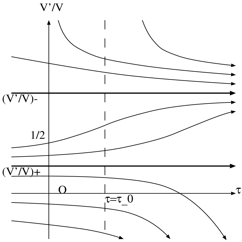
FIG. 2.: Dynamical behavior of the kink mode for a nondegenerate-nodal sonic point. The figure is the same except for $(V^{\prime}/V)_{+}<0$ for a saddle sonic point.

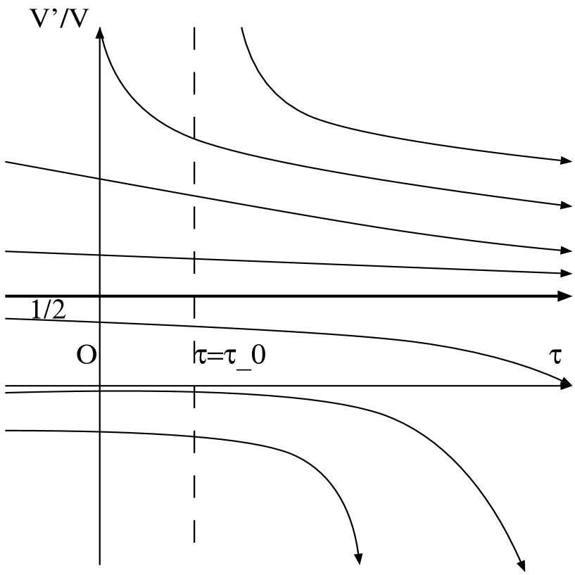
FIG. 3.: Dynamical behavior of the kink mode for a degenerate-nodal sonic point.