On the possibility of an astronomical detection of chromaticity effects in microlensing by wormhole-like objects

Abstract

We study the colour changes induced by blending in a wormhole-like microlensing scenario with extended sources. The results are compared with those obtained for limb darkening. We assess the possibility of an actual detection of the colour curve using the difference image analysis method.

1 Introduction

This paper continues our study on the possible observational effects that struts of negative masses would produce if they are isolated in space [1]. Since wormhole structures require the violation of some of the most sensitive energy conditions at the wormhole throat, wormholes are natural candidates –if they exist at all– for stellar size negative mass objects. Different wormhole solutions have been presented in the literature after the leading work of Morris and Thorne [2] (see for example Refs. [3]). Many of these solutions actually present a negative energy density and open the possibility of having a total negative mass. However, only a few works deal with the problem of developing observational tests for the existence of wormhole-like objects. Our aim in the present series of papers is to turn the speculation on macroscopic amounts of negative masses into an experimental question, one whose answer could be reached by current astrophysical observations.

In a recent paper [4], we have studied the gravitational microlensing scenario that a negative mass point lens would produce over an extended source. This allowed us to present more realistic light curves for wormhole microlensing events than those obtained earlier by Cramer et al. [5]. Using the formalism introduced in Refs. [6], we computed the effects of a finite source extent on the spectral features of microlensing. We showed that limb darkening of the intensity distribution on a stellar source induces specific chromaticity effects that are very different from what is expected in the positive mass lens case. The possibility of using multi-colour optical observations to search for galactic or inter-galactic natural wormhole-like objects was then foreseen.

Detection of the extended source effects from colour measurements, instead of single band photometry, is interesting because of two facts (see Ref. [7] for further discussion). Firstly, by detecting the colour curves the extended nature of the source is revealed: if the source approaches very close to the lens caustics but do not cross them, the induced amplification can always be mimicked by changes in the lensing parameters of a point-like object. By contrast, the colour curves can not be mimicked by any such changes: a point source lensing event should always be achromatic. Secondly, the colour curve allows one to measure the lens proper motion quite easily, without the need of fitting the entire light curve.

However, measurements of the colour curve can actually be hampered by light blending caused from nearby and background sources, which also causes chromaticity effects. Han et al. [6] have demonstrated that even for a small fraction (less than 2%) of blended light, the colour changes caused by blending can be equivalent in magnitude to those caused by limb-darkening. Therefore, in order to get predictions for a colour curve, it is essential to take blending into account, and to remove, somehow, its effects.

In the present letter we shall analyze the chromaticity effects produced, in the case of a wormhole-like microlensing event, by blending of other stars. In addition, we shall estimate the likelihood of carrying out an actual observation of the colour curves using the difference image analysis method within current technological capabilities.

2 A brief summary of microlensing formulae

The amplification produced by gravitational lensing of a point source is given by [5]

$$A_{0}=\frac{B_{0}^{2}\pm 2}{B_{0}\sqrt{B_{0}^{2}\pm 4}},$$ (1)

where the plus sign corresponds to positive mass and the minus sign to negative mass lensing, and $B_{0}=b_{0}/R_{E}$ is the lens-source separation in units of the Einstein radius $R_{E}$,

$$R_{E}=\sqrt{\frac{4G|M|}{c^{2}}\frac{D_{ol}D_{ls}}{D_{os}}}.$$ (2)

As usual, $D_{os}$ is the observer-source distance, $D_{ol}$ is the observer-lens distance, $D_{ls}$ is the lens-source distance, and $M$ the mass of the gravitational lens. For an extended circular source, instead, the light curve is given by [4]

$$A=\frac{\int_{0}^{2\pi}\int_{0}^{r_{*}}{\mathcal{I}}(r,\varphi)A_{0}(r,\varphi)rdrd\varphi}{\int_{0}^{2\pi}\int_{0}^{r_{*}}{\mathcal{I}}(r,\varphi)rdrd\varphi}.$$ (3)

Here, $(r,\varphi)$ are polar coordinates in a reference frame placed in the center of the star, $r_{*}$ is the radius of the source, and ${\mathcal{I}}(r,\varphi)$ is its surface intensity distribution. For a radially symmetric distribution, the previous expression transforms into (defining the dimensionless radius $R=r/R_{E}$)

$$A=\frac{\int_{0}^{2\pi}\int_{0}^{R_{*}}{\mathcal{I}}(R)A_{0}(R,\varphi)RdRd\varphi}{2\pi\int_{0}^{R_{*}}{\mathcal{I}}(R)RdR},$$ (4)

where $R_{*}=r_{*}/R_{E}$ is the dimensionless radius of the star. If the lens is moving with constant velocity $v$, the lens-source separation (in units of the Einstein radius) is given by

$$B(T)=\frac{b(t)}{R_{E}}=\sqrt{\left(B_{0}+R\sin\varphi\right)^{2}+\left(-T+R\cos\varphi\right)^{2}},$$ (5)

where $T=vt/R_{E}$ (see Ref. [4] for a helpful plot and further details). Replacing $B_{0}$ in Eq. (1) by its time-dependent partner, $B(T)$, and using this expression in Eq. (4), we arrive, for a given intensity distribution ${\mathcal{I}}(R)$, at the light curves produced by lensing in an extended source case.

3 Blending

The obscuration of the intensity profile of a star towards its border is known as limb darkening. An extended source microlensing event become chromatic as a consequence of this effect, see for instance Ref. [6]. The colour change caused by limb darkening of the source star can be computed using [6]

$$\Delta(m_{\nu_{2}}-m_{\nu_{1}})=-2.5\log\left(\frac{A_{\nu_{2}}}{A_{\nu_{1}}}\right),$$ (6)

where $A_{\nu_{1}}$ and $A_{\nu_{2}}$ are the amplifications in two different wavelength bands, $\nu_{1}$ and $\nu_{2}$. For the intensity profile we shall take, in terms of the radius $R$, and as in Refs. [4, 6],

$${\mathcal{I}}_{\nu}(R)=1-C_{\nu}\left(1-\sqrt{1-\left(\frac{R}{R_{*}}\right)^{2}}\right),$$ (7)

with the limb-darkening coefficients $C_{\nu_{1}}=0.503$ , $C_{\nu_{2}}=1.050$ corresponding to the I and U bands of a K-giant with $T_{{\rm eff}}=4750K$.

But the light curve of a microlensing event can also be chromatic by another effect: blending. Basically, the light flux of a source star can be affected by blended light of other unresolved stars, having themselves different colours, what results in a change of the colour curve. If we consider both effects at the same time, limb darkening and blending, the so generated colour curve was recently computed by Han et al. [7] to be

$$\Delta(m_{\nu_{2}}-m_{\nu_{1}})=-2.5\log\left[\left(\frac{A_{\nu_{2}}+f_{\nu_{2}}}{A_{\nu_{1}}+f_{\nu_{1}}}\right)\left(\frac{1+f_{\nu_{2}}}{1+f_{\nu_{1}}}\right)^{-1}\right],$$ (8)

where $f_{\nu_{i}}$ are the fractions of the blended light in the individual wavelength bands. These fractions depend on the specific situation and will be different for different backgrounds. The colour changes due only to the blending effect will be the difference between the colour curve of the limb darkening event affected by blending (Eq. 8) and the colour curve for limb darkening alone (given in Eq. (6) and Ref. [4]). To ease the comparison with the standard (i.e. possitive mass) case, we shall adopt the blending coefficients as $f_{U}=1.39\%$ and $f_{I}=1.04\%$, and a source star with radius $R_{*}=0.1$ [7]. Our new results, including the effect of blending, and for different impact parameters $k=b_{0}/r_{*}=B_{0}/R_{*}$, are shown in Figures 1 and 2.

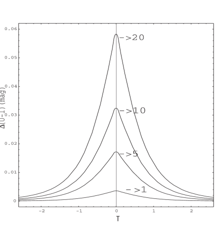
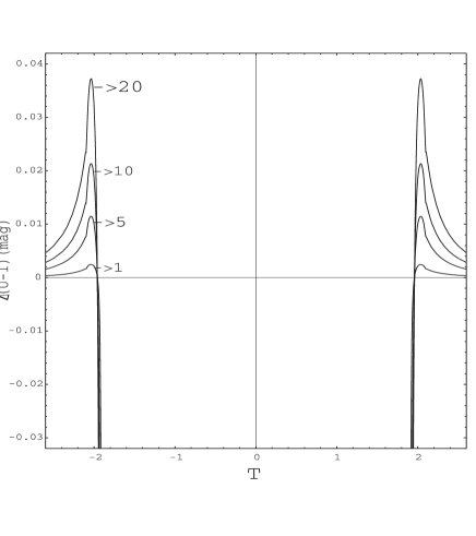
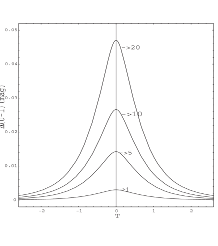
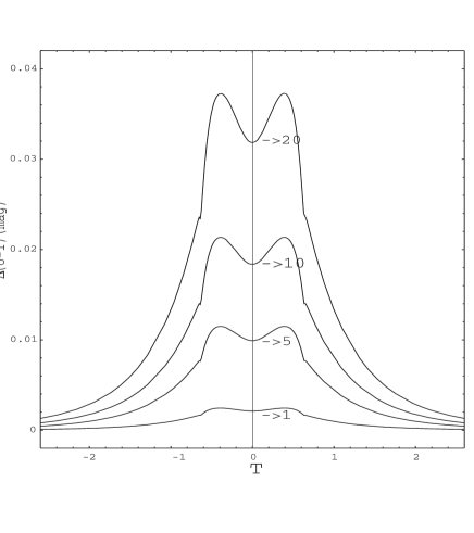
Figure 1: Colour changes produced by blending in microlensing events. The number of blended stars is shown in each curve. Upper left: Positive lensing, impact parameter $k=b_{0}/r_{*}=0.5$. Upper right: Negative lensing, same impact parameter. Bottom Left: Positive lensing, $k=2$. Bottom right: Negative lensing, $k=20$. The source star has dimensionless radius $R_{*}=0.1$.

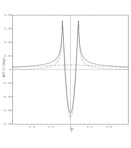
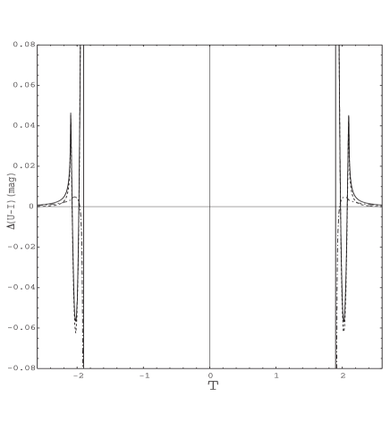
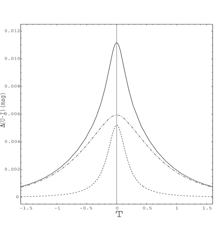
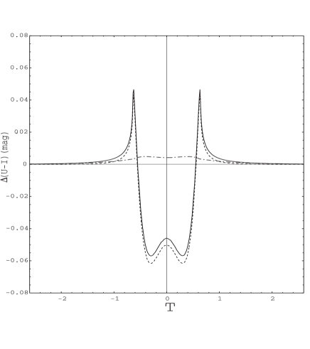
Figure 2: Full and partial contributions to chromaticity effects in microlensing. The solid line is the full colour curve of an event affected by blending (two blended stars), the dash curve represents the colour curve if the same event is not affected by blending, whereas the dash-dot curve gives only the colour changes due to the blending effect. Upper Left: Positive lensing, impact parameter $k=b_{0}/r_{*}=0.5$. Upper right: Negative lensing, same impact parameter. The umbra is no longer present, but rather there is a plateau ($\Delta(U-I)\approx-0.31$), that dominates the umbra region in the colour curves, produced only by the blended light. This plateau is not shown in the figure in order to show the detail in the upper portions of the colour curve. Bottom Left: Positive lensing, $k=2$. Bottom right: Negative lensing, $k=20$. The source star has dimensionless radius $R_{*}=0.1$.

The colour curves without blending present an umbra region in the negative lensing case (no light reaches the observer) when the impact parameter is small ($k<20$) [4]. Considering blending, instead, we now discover that this umbra is no longer present, but rather that there is a ‘plateau’ ($\Delta(U-I)\approx-0.31$) in the colour curves, produced only by the blended light. This plateau is not directly shown in the figures in order to show the detail in the upper portion of the colour curve. This new effect has important implications in the full colour curves, as Figure 2 shows.

In the case of an ordinary lens, the colour curves affected by blending are very similar to the photometric ones, see [4] for a comparison. We see that as it gets closer to the star, the color of the observed source becomes redder due to the differential amplification of the coldest regions. When the lens transits towards the star interior, the hot center starts to dominate the amplification, producing a dramatic change in the slope.

For the limb darkening colour curve (dash curve in Figure 2), the spectral changes start long before than in the standard situation. Initially, the source also becomes redder and then experiences a switch when shorter wavelengths begin to dominate. Contrary to what happens with positive masses, the spectral trend changes again, with the source appearing colder and colder until it vanishes in the umbra during the transit. When the source is seen again, the inverse behaviour is observed. If we now take into account the blending effect as well, the existence of the previously mentioned plateau, instead of the umbra region, make the colour curve to change its trend again, towards the blue region. During the transit, it is the blended contribution the one that dominates the colour curve. It makes sense: blending fluxes come from stars whose light is not deflected by the wormhole-like object, and so the typical umbra effect is absent. Blending, then, and contrary to the positive mass case (where the pattern of the colour curve is maintained with only slight changes in the actual values for $\Delta(U-I)$), noticeably affects the form of the colour curve in a wormhole-like microlensing event.

The difference between the negative and the positive colour curves (that we show for comparison in the same set of figures) continues to be very clear, and hence, these combined effects allow to distinguish between the different kind of lenses. We shall now focus on demonstrating that the colour curve can actually be observed with current technology in typical cases.

4 The DIA colour curve

The difference image analysis (DIA) is a method to measure blending-free light colour variations by subtracting an observed image from a convolved and normalized reference one. The flux would then be, within DIA,

$$F_{\nu}=F_{\nu,{\rm obs}}-F_{\nu,{\rm ref}}=(A_{\nu}-1)F_{\nu,0},$$ (9)

where $F_{\nu,{\rm obs}}=A_{\nu}F_{\nu,0}+B_{\nu}$ and $F_{\nu,{\rm ref}}=F_{\nu,0}+B_{\nu}$ stand for the source star fluxes measured from the images obtained during the progress of the microlensing event, and from the reference (unlensed) image, respectively. $B_{\nu}$ is the blended flux. Then, the DIA colour curve is given by [7]

$${\Delta(m_{\nu_{2}}-m_{\nu_{1}})}_{DIA}=-2.5\log\left[\left(\frac{A_{\nu_{2}}(t)-1}{A_{\nu_{1}}(t)-1}\right)\left(\frac{A_{\nu_{2}}(t_{{\rm ref}})-1}{A_{\nu_{1}}(t_{{\rm ref}})-1}\right)^{-1}\right].$$ (10)

The advantage of measuring this curve, instead of that given by Eq. (8), is that it does not depend on the blending parameters $f_{\nu,i}$ (equivalently, $B_{\nu,i}$). We shall choose $t_{{\rm ref}}$ from the condition

$${\Delta(m_{\nu_{2}}-m_{\nu_{1}})}_{DIA}=0,$$ (11)

when the reference star suffers no amplification. Basically, $t_{{\rm ref}}\rightarrow\infty$. Again, we shall fix our attention to the U and I bands of a K-giant source star with dimensionless radius $R_{*}=0.1$ and $T_{{\rm eff}}=4750K$. The results for positive and negative lensing with different impact parameters $k=b_{0}/r_{*}=B_{0}/R_{*}$ are shown in Figure 3.

Even when the DIA colour curve can have a different form when compared with that produced only by limb-darkening, they both depend on the same parameters, $A_{\nu_{1}}$ and $A_{\nu_{2}}$. Hence, the same information can be extracted from both curves, but with significantly reduced uncertainties in the DIA case, because of the absence of blending.

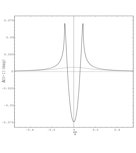
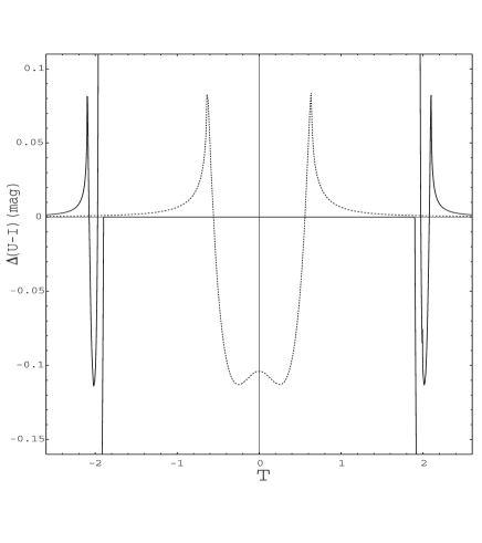
Figure 3: DIA colour curves. Left: Positive lensing, impact parameter $k=b_{0}/r_{*}=0.5$ (solid curve) and $k=2$ (dash curve). Right: Negative lensing, $k=0.5$ (solid curve) and $k=20$ (dash curve). The source star has dimensionless radius $R_{*}=0.1$.

It is interesting to directly compare, then, the DIA colour curve just presented with the limb-darkening photometric curve presented in Figure 3b of Ref. [4], or here in the right panels of Figure 2, dash lines. The analytical difference between both colour curves reduces itself to the replacement

$$\frac{A_{\nu_{2}}}{A_{\nu_{1}}}\rightarrow\frac{A_{\nu_{2}}-1}{A_{\nu_{1}}-1}$$ (12)

within the logarithm function used in the magnitude definition. This apparently simple change has, however, large implications for the negative mass colour curve when $k<20\;\;(b_{0}<2R_{E})$. Particularly, when either $A_{\nu_{1}}$ or $A_{\nu_{2}}$ are less than 1, but not both, the ratio $(A_{\nu_{2}}-1)/(A_{\nu_{1}}-1)$ is less than zero, yielding a not defined colour change. This happens just before the umbra, when large variations in the amplification suddenly occur at slightly different times for different frequencies, this being the reason of the apparent extra cusp in the DIA colour curve. We show the behaviour of the ratio $(A_{\nu_{2}}-1)/(A_{\nu_{1}}-1)$ for our two particular frequencies in Figure 4.

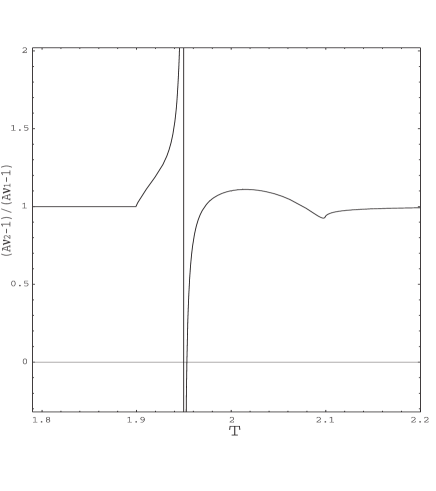
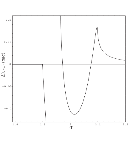
Figure 4: Left: Example of the partial evolution of the ratio $(A_{\nu_{2}}-1)/(A_{\nu_{1}}-1)$ in the case of negative mass lensing. Right: DIA colour curve in the same temporal interval. Impact parameter is $k=0.5$, and $R_{*}=0.1$, for both figures.

Interestingly, the positive mass DIA curve is completely similar to the photometric one, since there is no time at which $A_{\nu_{1}}-1$ and $A_{\nu_{2}}-1$ have a different sign.

The behavior of the negative DIA colour curve deserves further study. In order to explore exactly the form of the curve that could actually be measured, we would need to implement a numerical code with a given binning in time (corresponding to a given integration time of a telescope). If one of the cusps in the colour curve is produced only by a single point, we might lose it in the binning process, but we shall shed some light on the behavior that could actually be observed. We have then adapted the numerical code used in Refs. [7] to the case of negative mass lenses. Figure 5 shows two particular examples obtained with this code. These curves show the qualitative expected behavior in its full extent.

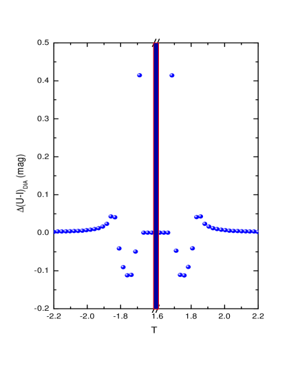
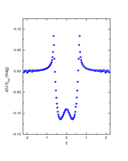
Figure 5: Negative mass DIA colour curves obtained with a numerical code, by binning the time interval for an impact parameter $k=10$ (left) and $20$ (right). The left hand side presents a break on the $x$-axis of the colour curve, where the umbra is located, in order to provide extra details. The source star has dimensionless radius $R_{*}=0.1$.

5 Measuring the DIA colour curve

Although the colour changes are usually small, they can be measured within current technological limitations. Following Han et al. [7], we write the uncertainty in the determined source star flux as related to the signal-to-noise ratio by

$$\delta m_{\nu}=\frac{\delta F_{\nu,0}/F_{\nu,0}}{0.4\ln 10}=\frac{1.09}{S/N}.$$ (13)

Then, the uncertainty in the measured colour is related as well to $S/N$ by

$$\delta\left[\Delta\left(m_{\nu_{2}}-m_{\mu_{\nu_{1}}}\right)_{DIA}\right]\sim\sqrt{2}\delta m_{\nu}\sim\frac{1.54}{S/N}.$$ (14)

If $S/N=10$, $\delta\left[\Delta\left(m_{\nu_{2}}-m_{\mu_{\nu_{1}}}\right)_{DIA}\right]\sim 0.15$. The signal measured from the substracted image is proportional to the source flux variation,

$$S\propto(A_{\nu}-1)F_{0,\nu}t_{\rm exp},$$ (15)

where $t_{\rm exp}$ is the exposure time. The noise comes from the lensed source as well as from the the blended background stars [7],

$$N\propto[A_{\nu}F_{0,\nu}+B]^{1/2}t_{exp}^{1/2},$$ (16)

where $B$ represents the average total flux of unresolved stars within a seeing disc of radius $\theta_{\rm seeing}$. Then, the signal to noise ratio is given by

$$S/N=(A_{\nu}-1)F_{0,\nu}\left(\frac{t_{\rm exp}}{A_{\nu}F_{0,\nu}+B}\right)^{1/2}.$$ (17)

Since we want to compare our error estimates with those corresponding to a positive case, we shall assume mutatis mutandis all parameters used in the discussion of the latter in Section 5 of Ref. [7].

Let us first take the source size as 0.07 Einstein radii, and the Einstein time scale as 67.5/2 days [7]. The lensed source is a K-star with I=14.05 mag. Observations are assumed to be carried with a 1m-telescope with a CCD camera that can detect 12 photons per second for a I=20 mag star. The exposure, $t_{\rm exp}$, is considered variable so as to allow for the measured signal to be $\sim 4\;10^{4}$ photons, which is in the range of the linear regime response in modern CCD cameras. Actually,

$$t_{exp}=\frac{4\;10^{4}{\rm photons}}{A_{\nu}F_{0,\nu}},$$ (18)

and so it will be different for each given magnification. The estimation of $B$ is done by assuming that blended light comes from stars fainter (i.e. with greater magnitudes) than the crowding limit, set when the stellar number density reaches $\sim 10^{6}$ stars deg^-2. This number density corresponds to $I\sim 18.1$ [7]. The background flux is normalized for stars in the seeing disc with $\theta_{seeing}=2$ arcsec. In the case of a positive lens, the exposure time required to achieve the requested flux of $10^{4}$ photons is only about some seconds, and this happens due to the huge magnifications that the lensing produces (up to 20 times around $t=0$).

In the negative mass lensing situation, the overall presence of the umbra dominates part of the error estimation as well. In particular, for magnifications less than 1, the $S/N$ is not well defined, since it becomes negative. But this happens just before the umbra, for only one point in the binned plot, and do not affect the correct estimate of the previously rising curve (on the left of the umbra, for instance). In addition, there is no sense in assigning an error to an absent signal, the umbra. We find that $S/N$ for the negative case can be around 80, with exposures times slightly larger than in the positive mass case, of about 8–10 s. This difference is produced by generically lower values for the magnification, which is of order 1, instead of the range 10–20 reached in the positive mass situation. In Figure 6 we show the case of $k=0.9$. Note that the natural scale for microlensing, the Einstein time scale, represents half the physical time spread in the $x$-axis of the left panel in Figure 6. Then, the negative mass lens has a longer time evolution, since the particular peak we are showing happens already in a time scale for which almost the complete microlensing event occurs in the positive mass case. In Figure 7 we show the cases of impact parameters $k=10$ and $k=20$, for which we have previously investigated the colour curve. Interestingly, due to small values of the amplification for the earliest or the latest times, the error significantly increases in these regions. This can be noticed particularly on the right panel of Figure 7. Overall, it is clear, then, that within current observational capabilities we could be able to distinguish between ordinary and exotic lenses, through the analysis of gravitational microlensing chromatic effects.

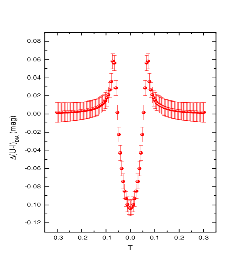
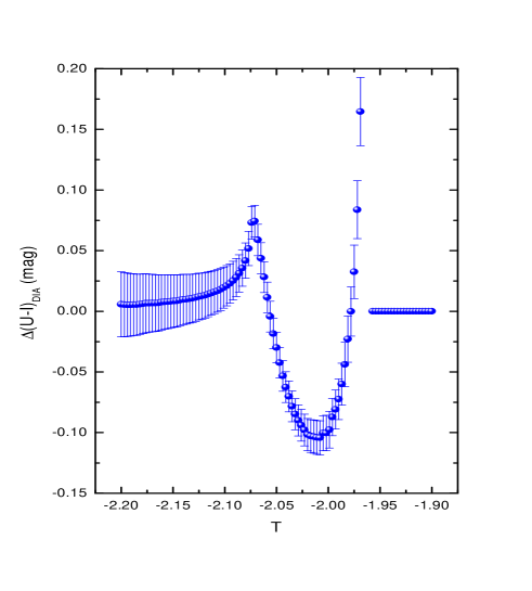
Figure 6: Left: Error estimate in the DIA colour curve for a positive lens, impact parameter $k=0.9$ and a source star with radius $R=0.07R_{E}$. Other parameters are discussed in the text. Right: Example of the error estimate in the partial evolution (left of the umbra) of the colour curve for a negative lens. Lensing parameters are the same as in the Left panel.

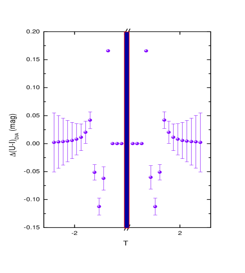
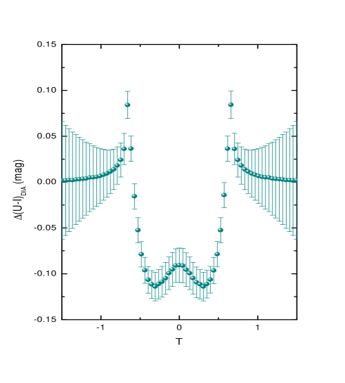
Figure 7: Error estimate in the DIA colour curve for negative lenses, impact parameter $k=10$ (again showing a break, left) and 20 (right), and a source star with radius $R=0.1R_{E}$.

At the moment, most of the microlensing experiments do not use the DIA method in their data analysis. However this is already beginning to change, see for instance Ref. [8], and will become a common practice in the near future. If the microlensing alert systems are adapted to take into account the possible colour and light curves produced by negative mass lenses, we shall be in position to make extensive searches –and to establish bounds on the possible existence– of wormhole-like objects.

6 Concluding remarks

All theoretical constructs thought to represent features of the real world should be queried through experimental or observational tests. This process is fundamental for science. In this paper, we have expanded the formalism for wormhole-like gravitational microlensing of extended sources by including the analysis of the effects of blending. Having so constructed a complete colour curve, taking into account the effects of limb darkening as well, we analyzed the possibilities for an actual detection of chromaticity effects.

Struts of negative masses, if they exist at all, will be detected through the effects they produce upon the light coming from distant sources. If a consistent lensing survey yields a negative result, we could then set empirical constraints from a statistical point of view to the amount of negative mass in the universe.

References

- [1] D. F. Torres, G. E. Romero & L. A. Anchordoqui, Phys. Rev. D58, 123001 (1998); D. F. Torres, G. E. Romero & L. A. Anchordoqui, (Honorable Mention, Gravity Foundation Research Awards 1998), Mod. Phys. Lett. A13, 1575 (1998); M. Safonova, G. E. Romero & D. F. Torres, Mod. Phys. Lett. A16, 153 (2001) [astro-ph/0104075]; L. A. Anchordoqui, G. E. Romero, D. F. Torres & I. Andruchow, Mod. Phys. Lett. A14, 791 (1999); G.E. Romero, D.F. Torres, L.A. Anchordoqui, I. Adruchow, B. Link, Monthly Notices Royal Astron. Soc. 308, 799 (1999); M. Safonova, G. E. Romero & D. F. Torres, [gr-qc/0105070]; L. A. Anchordoqui, S. Capozziello, G. Lambiase & D. F. Torres, Mod. Phys. Lett. A15, 2219 (2000).
- [2] M. S. Morris & K. S. Thorne, Am. J. Phys. 56, 395 (1988).
- [3] D. Hochberg & M. Visser, Phys. Rev. Lett. 81, 746 (1998); Phys. Rev D58, 044021 (1998); Phys. Rev. D56, 4745 (1997); E. E. Flanagan & R. M. Wald, Phys. Rev. D54, 6233 (1996); L. A. Anchordoqui, S. E. Perez Bergliaffa & D. F. Torres, Phys. Rev. D55, 5226 (1997); C. Barceló & M. Visser, Phys. Lett. B466, 127 (1999); A. DeBenedictis & A. Class.Quant.Grav. 18, 1187 (2001); S. E. Perez Bergliaffa & K. E. Hibberd, Phys. Rev. D 62, 044045 (2000); L. A. Anchordoqui & S. E. Perez Bergliaffa, Phys. Rev. D 62, 067502 (2000); D. Hochberg, A. Popov, & S. V. Sushkov, Phys. Rev. Lett. 78, 2050 (1997); S. Kim & H. Lee, Phys. Lett. B 458, 245 (1999); S. Krasnikov, Phys. Rev. D 62, 084028 (2000).
- [4] E. F. Eiroa, G. E. Romero, & D. F. Torres, Modern Physics Letters A16, 973 (2001).
- [5] J. G. Cramer, R. L. Forward, M. S. Morris, M. Visser, G. Benford, G. A. Landis, Phys. Rev. D51, 3117 (1995).
- [6] C. Han, S-H. Park, J-H. Jeong, Monthly Notices Royal Astron. Soc. 316, 97 (2000).
- [7] C. Han, & S-H. Park, Monthly Notices Royal Astron. Soc. 320, 41 (2001).
- [8] P.R. Wozniak et al., Difference image analysis of the OGLE-II bulge data II: Microlensing events, astro-ph/0106474.